A Heterogeneous Duopoly Game under an Isoelastic Demand and Diseconomies of Scale

Abstract

In this paper, we investigate a duopolistic market with heterogeneous firms under the assumptions of an isoelastic demand and quadratic costs. We obtain the sufficient and necessary condition of the local stability of the Cournot–Nash equilibrium and analytically compare it with that of the analogue model under linear rather than quadratic costs. By approaches of symbolic computation, we prove that diseconomies of scale have an effect of stabilizing the game provided that the cost parameters are large enough. Moreover, by means of numerical simulations, we find that our model loses its stability only through a period-doubling bifurcation, which is different from its analogue having two possible routes to chaotic dynamics.

1. Introduction

There are two common market structures: perfect competition and monopoly. In the first case, the market has many relatively small companies competing with each other. In the second case, one single supplier takes over the whole market. Between these two cases, there exists another market form called oligopoly, where a small number of firms produce identical products. It is well-known that Cournot [1] first introduced the formal oligopoly theory in 1838. In his seminal work, a static duopoly model was investigated, where each firm is supposed to have perfect information about its rival’s strategic behavior.

Since then, a number of dynamic oligopoly games have been explored, where the market demand function is usually supposed to be linear, e.g., [2,3]. However, the assumption of a linear demand function is not always realistic. To address this concern, Puu [4] proposed a discrete Cournot duopoly model under an isoelastic market demand curve with price simply the reciprocal sum of two firms’ outputs and showed that complex dynamics such as periodic orbits and chaos could easily take place. A lot of studies are motivated by Puu’s work, e.g., [5,6,7,8,9,10,11,12], with many fruitful and interesting results in the direction of investigating complicated dynamics of various duopoly models, where the modern mathematics of nonlinear dynamics and complexity theory has been intensively applied.

In the literature on oligopolistic games, a homogeneous oligopoly often refers to an oligopoly game where firms adopt identical strategies to adjust their behavior. In comparison, a heterogeneous oligopoly model employs the assumption that the players use different rules to decide their behavior. The latter is more realistic since it is rare that different firms behave according to the same rules among a large number of possible strategies. In ecology, it is well-known that it is impossible for species with identical niches can coexist indefinitely according to the competitive exclusion principle. This principle also applies to economics. In the real economy, we often observe that companies with different business strategies coexist in the same industry due to different risk preference and asymmetric information. But, homogeneous firms in a number of industries, e.g., the Internet industry, can just coexist temporarily before the state of the economic system reaches the equilibrium. In this regard, our work focuses on the heterogeneous duopoly game by coupling a gradient adjusting mechanism with a naive expectation mechanism.

In this paper, we employ the same isoelastic demand function as Puu’s model [4], but we introduce nonlinear cost functions to investigate how diseconomies of scale affect the dynamic behavior of a heterogeneous duopoly game with a boundedly rational player and a naive player. Under the same demand but linear cost functions, the analogue of our model has been investigated by Tramontana [13]. However, in our model, the two duopolists are assumed to have quadratic costs, which may be important in several applications. For instance, Bischi and others [14] proposed a fishery model based on a Cournot oligopoly game where n profit-maximizing players harvest fish and sell their catch on several markets. They used a Cobb–Douglas production function with fishing effort and fish stock as the two inputs and derived that the harvesting costs depend on the square of the harvested quantity. The nonlinearity of firms’ costs permits us to extend the applications of the Cournot theory to oligopolistic markets under diseconomies of scale. Related to our research is [3], where Dubiel-Teleszynski studied a heterogeneous Cournot duopoly game with boundedly rational and adaptive players. The difference is that a linear rather than an isoelastic demand function is used in Dubiel-Teleszynski’s model.

Using approaches of symbolic computation [15], we find that, if the cost parameters are large enough, diseconomies of scale have an effect of stabilizing the heterogeneous duopoly game considered in this paper. This finding is consistent with the result discovered by Fisher [2] as well as by McManus and Quandt [16], that increasing marginal cost is a stabilizing influence for oligopolies with n players. It should be mentioned that these studies considered only homogeneous mechanisms of adjusting firms’ outputs and a linear demand function. However, we introduce heterogeneous agents and a nonlinear demand to our study. In contrast, Dubiel-Teleszynski’s opposite conclusion that industries facing diseconomies of scale are less stable than those with constant marginal costs surprises us. Specifically, Dubiel-Teleszynski [3] found that the region of stability of his model under the framework of increasing marginal costs is smaller than its analogous game found by Agiza and Elsadany [17] under linear instead of quadratic cost functions. In addition, this paper unveils another crucial difference between our model and its analogue by Tramontana [13]: our model loses its local stability only through a period-doubling bifurcation, but for Tramontana’s, there exist two possible routes, through a period-doubling bifurcation and a Neimark–Sacker bifurcation, to complicated dynamics.

Our study contributes to the literature on dynamic oligopoly models in two ways, i.e., the modeling and the methodology. On the one hand, we explore a duopoly game under the assumptions of an isoelastic demand function and quadratic costs. It becomes complicated to investigate oligopoly models when the market demand is nonlinear and firms’ costs are also nonlinear. To our knowledge, such a model setting is seldom adopted in the previous literature. On the other hand, we introduce several methods of symbolic computation, e.g., the triangular decomposition and the partial cylindrical algebraic decomposition, into the study of dynamics of oligopoly games. We show that symbolic computation methods could be powerful tools in theoretical economics, such as theorem proving (see, e.g., the proof of Corollary 1).

The rest of this paper is structured as follows. In Section 2, we propose a heterogeneous duopoly model under the assumptions of an isoelastic demand and diseconomies of scale. In Section 3, the unique equilibrium and its local stability of the proposed duopoly are thoroughly investigated. The stability regions of our model and its analogue with linear costs are compared analytically and graphically. In Section 4, numerical simulations are performed to explore complex dynamics such as periodic solutions and chaos of our game. The paper is concluded with some remarks in Section 5.

2. Model

Let us consider a market with two firms producing identical products. Let $q_1\left(t\right)$ and $q_2\left(t\right)$ denote the outputs of the two firms, respectively, at period t. We assume that the market is featured by an isoelastic demand function as in Puu [4], which is based on the hypothesis of the Cobb–Douglas utility function by the agents. Specifically, the market inverse demand function is

$$p\left(Q\right)=\frac{1}{Q}=\frac{1}{q_1+q_2},$$

where $Q=q_1+q_2$ is the total market supply. Moreover, the cost function of firm i is assumed to be quadratic, i.e.,

$$C_1\left(q_1\right)=c_1{q}_1^2,C_2\left(q_2\right)=c_2{q}_2^2,$$

where $c_1>0$ and $c_2>0$ can be seen as shift parameters in these cost functions, respectively. Then the marginal costs of the two firms are

$$M{C}_1\left(q_1\right)=2c_1{q}_1,M{C}_2\left(q_2\right)=2c_2{q}_2,$$

which are increasing as the outputs $q_1$ and $q_2$ grow. That is, we say that these two players have increasing marginal costs or diseconomies of scale.

Under the above assumptions, the profit of firm i at period t would be

$${\Pi }_i\left(t\right)=\frac{q_i\left(t\right)}{q_i\left(t\right)+q_{-i}\left(t\right)}-c_i{q}_i^2\left(t\right),i=1,2,$$

where $q_{-i}\left(t\right)$ represents the output of the rival at period t. As a result, the marginal profit of firm i is

$$\frac{\partial {\Pi }_i\left(t\right)}{\partial q_i\left(t\right)}=\frac{q_{-i}\left(t\right)}{{(q_i\left(t\right)+q_{-i}\left(t\right))}^2}-2c_i{q}_i\left(t\right).$$

Solving the first order condition, i.e., $\partial {\Pi }_i\left(t\right)/\partial q_i\left(t\right)=0$, each firm could maximize its own profit. In the real world, however, it is appropriate to assume that firms cannot obtain their competitors’ production information in advance, which means that $q_{-i}(t+1)$ is unknown at period $t+1$.

In our study, the two firms are assumed to adopt heterogeneous strategies of adjusting their outputs. We suppose that the first firm is a boundedly rational player, which increases/decreases its output according to the information given by the marginal profit of the last period. In particular, firm 1 could adjust its output at period $t+1$ with a gradient mechanism (also called the myopic adjusting mechanism or the rule of thumb) as

$$q_1(t+1)=q_1\left(t\right)+K{q}_1\left(t\right)\frac{\partial {\Pi }_1\left(t\right)}{\partial q_1\left(t\right)},$$

i.e.,

$$q_1(t+1)=q_1\left(t\right)+K{q}_1\left(t\right)\left[\frac{q_2\left(t\right)}{{(q_1\left(t\right)+q_2\left(t\right))}^2}-2c_1{q}_1\left(t\right)\right]$$

where $K>0$ is a parameter controlling the adjustment speed. It is worth noting that the adjustment speed depends upon not only the parameter K but also the size of the first firm $q_1\left(t\right)$. One may observe that a boundedly rational player does not need to expect or guess the output of its rival at the current period.

The second firm, instead, is a naive player, who naively expects the output of its rival at the current period $t+1$ is the same as that of the last period. Therefore, the expected profit at period $t+1$ is

$${\Pi }_2^e(t+1)=\frac{q_2(t+1)}{q_2(t+1)+q_1\left(t\right)}-c_2{q}_2^2(t+1),$$

and its marginal profit is

$$\frac{\partial {\Pi }_2^e(t+1)}{\partial q_2(t+1)}=\frac{q_1\left(t\right)}{{(q_2(t+1)+q_1\left(t\right))}^2}-2c_2{q}_2(t+1).$$

The first order condition for profit maximization yields a cubic polynomial equation, i.e.,

$$q_1\left(t\right)-2c_2{q}_2(t+1){(q_2(t+1)+q_1\left(t\right))}^2=0.$$

(1)

The second firm could maximize its expected profit by solving the above equation. One can verify that there exists a unique real solution for $q_2(t+1)$ of (1), but its closed-form expression is quite complex,

$$q_2(t+1)=\frac{\sqrt[3]{2}M}{6c_2}+\frac{\sqrt[3]{4}{c}_2{q}_1^2\left(t\right)}{3M}-\frac{2q_1\left(t\right)}{3},$$

(2)

where

$$M=\sqrt[3]{c_2^2{q}_1\left(t\right)\left(4c_2{q}_1^2\left(t\right)+3\sqrt{3}\sqrt{8c_2{q}_1^2\left(t\right)+27}+27\right)}.$$

For simplicity, we denote (2) as

$$q_2(t+1)=R_2\left(q_1\left(t\right)\right),$$

where $R_2$ is called the best response function of the second firm.

In short, the model is described as the following two-dimensional iteration map.

$$\left\{\begin{array}{cc}\hfill q_1(t+1)=& q_1\left(t\right)+K{q}_1\left(t\right)\left[\frac{q_2\left(t\right)}{{(q_1\left(t\right)+q_2\left(t\right))}^2}-2c_1{q}_1\left(t\right)\right],\hfill \\ \hfill q_2(t+1)=& R_2\left(q_1\left(t\right)\right).\hfill \end{array}\right.$$

(3)

It should be noted that this map is not defined on the origin $(0,0)$.

3. Local Stability

In order to identify the equilibrium, we set $q_1(t+1)=q_1\left(t\right)=q_1^{*}$ and $q_2(t+1)=q_2\left(t\right)=q_2^{*}$. Then

$$\left\{\begin{array}{c}K{q}_1^{*}\left[\frac{q_2^{*}}{{(q_1^{*}+q_2^{*})}^2}-2c_1{q}_1^{*}\right]=0,\hfill \\ q_2^{*}=R_2\left(q_1^{*}\right).\hfill \end{array}\right.$$

(4)

We acquire the following result.

Theorem 1.

The iteration map (3) has one unique equilibrium:

$$E_1=\left[\frac{\sqrt[4]{c_2}}{\sqrt{2}\left(\sqrt{c_1}+\sqrt{c_2}\right)\sqrt[4]{c_1}},\frac{\sqrt[4]{c_1}}{\sqrt{2}\left(\sqrt{c_1}+\sqrt{c_2}\right)\sqrt[4]{c_2}}\right].$$

Proof. 

Recalling that (2) is derived from (1), we know $q_2^{*}=R_2\left(q_1^{*}\right)$ is equivalent to

$$q_1^{*}-2c_2{q}_2^{*}{(q_2^{*}+q_1^{*})}^2=0.$$

(5)

Moreover, it is satisfied that

$$K{q}_1^{*}\left[\frac{q_2^{*}}{{(q_1^{*}+q_2^{*})}^2}-2c_1{q}_1^{*}\right]=0,$$

thus two possible cases should be considered. If $q_1^{*}=0$, then (5) implies that $q_2^{*}=0$, which is impossible as map (3) is not defined on the origin $(0,0)$. If $q_1^{*}\ne 0$, then we have $\frac{q_2^{*}}{{(q_1^{*}+q_2^{*})}^2}-2c_1{q}_1^{*}=0$, which means $q_2^{*}-2c_1{q}_1^{*}{(q_1^{*}+q_2^{*})}^2=0$. One can obtain the following equations

$$\left\{\begin{array}{c}{q}_2^{*}=2c_1{q}_1^{*}{(q_1^{*}+q_2^{*})}^2,\hfill \\ q_1^{*}=2c_2{q}_2^{*}{(q_2^{*}+q_1^{*})}^2.\hfill \end{array}\right.$$

(6)

There is a simpler way of solving these two equations. Provided that $q_1^{*}\ne 0$ and $q_2^{*}\ne 0$, dividing the first equation by the second one, we know $q_2^{*}/q_1^{*}=c_1/c_2\times q_1^{*}/q_2^{*}$, from which $q_1^{*}=\sqrt{c_2/c_1}\times q_2^{*}$. Substituting this into (6), one can obtain the equilibrium $E_1$. However, this is a special case that this solving approach is feasible for we can deduce the simple relation $q_1^{*}=\sqrt{c_2/c_1}\times q_2^{*}$. Here, we want to show another way of computing the equilibrium using the triangular decomposition that is suitable for general polynomial equations. The triangular decomposition method can be viewed as an extension of the Gaussian elimination method. The main idea of these two methods is to transform an equation system into a triangular form. However, the triangular decomposition method is feasible for polynomial systems, while the Gaussian elimination method is only for linear systems. The readers can refer to [18,19,20,21,22] for more information on the triangular decomposition.

The triangular decomposition method permits us to decompose the solutions of (6) into zeros of the following two triangular sets

$$\begin{array}{cc}\hfill & T_1=\left[q_2^{*},q_1^{*}\right],\hfill \\ \hfill & T_2=\left[(4c_1{c}_2{q}_1^{{*}^2}-c_2)q_2^{*}+(2c_1^2+2c_1{c}_2)q_1^{{*}^3},(4c_1^3-8c_1^2{c}_2+4c_1{c}_2^2)q_1^{{*}^4}+8c_1{c}_2{q}_1^{{*}^2}-c_2\right].\hfill \end{array}$$

The zero of $T_1$ is redundant since map (3) is not defined on the origin $(0,0)$. The second polynomial $(4c_1^3-8c_1^2{c}_2+4c_1{c}_2^2)q_1^{{*}^4}+8c_1{c}_2{q}_1^{{*}^2}-c_2$ of $T_2$ is a univariate polynomial in $q_1^{*}$ and could be solved by

$$\begin{array}{cc}\hfill & \frac{\sqrt[4]{c_2}}{\sqrt{2}\left(\sqrt{c_1}+\sqrt{c_2}\right)\sqrt[4]{c_1}},\frac{-\sqrt[4]{c_2}}{\sqrt{2}\left(\sqrt{c_1}+\sqrt{c_2}\right)\sqrt[4]{c_1}},\hfill \\ \hfill & \frac{\mathrm{i}\sqrt[4]{c_2}}{\sqrt{2}\left(\sqrt{c_1}+\sqrt{c_2}\right)\sqrt[4]{c_1}},\frac{-\mathrm{i}\sqrt[4]{c_2}}{\sqrt{2}\left(\sqrt{c_1}+\sqrt{c_2}\right)\sqrt[4]{c_1}}.\hfill \end{array}$$

Among them, only the first solution $q_1^{*}=\frac{\sqrt[4]{c_2}}{\sqrt{2}\left(\sqrt{c_1}+\sqrt{c_2}\right)\sqrt[4]{c_1}}$ is economically meaningful. Substituting it into the first polynomial of $T_2$, we can easily compute $q_2^{*}=\frac{\sqrt[4]{c_1}}{\sqrt{2}\left(\sqrt{c_1}+\sqrt{c_2}\right)\sqrt[4]{c_2}}$. Therefore, the equilibrium $E_1$ is obtained. □

It is obvious that the unique equilibrium $E_1$ is the Nash equilibrium of our game, i.e., the Cournot–Nash equilibrium. Furthermore, the profits of the two firms corresponding to the Cournot–Nash equilibrium $E_1$ are

$${\Pi }_1^{*}=\frac{\sqrt{c_2}\left(c_1+2\sqrt{c_1{c}_2}\right)}{2\sqrt{c_1}{\left(\sqrt{c_1}+\sqrt{c_2}\right)}^2},{\Pi }_2^{*}=\frac{\sqrt{c_1}\left(c_2+2\sqrt{c_1{c}_2}\right)}{2\sqrt{c_2}{\left(\sqrt{c_1}+\sqrt{c_2}\right)}^2}.$$

We have

$$\frac{{\Pi }_1^{*}}{{\Pi }_2^{*}}=\frac{c_2(c_1+2\sqrt{c_1{c}_2})}{c_1(c_2+2\sqrt{c_1{c}_2})}.$$

If $c_1<c_2$, then

$$c_2{c}_1+2c_2\sqrt{c_1{c}_2}>c_1{c}_2+2c_1\sqrt{c_1{c}_2},$$

from which it is known that $\frac{{\Pi }_1^{*}}{{\Pi }_2^{*}}>1$ or ${\Pi }_1^{*}>{\Pi }_2^{*}$. In other words, a more efficient firm achieves a higher profit, and vice versa. It is consistent with our economic intuition.

In order to investigate the local stability of the equilibrium, we consider the Jacobian matrix of map (3), i.e.,

$$J(q_1,q_2)=\left[\begin{array}{cc}1-2K{c}_1{q}_1+K{\displaystyle \frac{q_2^2-q_1{q}_2}{{(q_1+q_2)}^3}}& K{\displaystyle \frac{q_1^2-q_1{q}_2}{{(q_1+q_2)}^3}}\\ {\displaystyle \frac{\mathrm{d}{R}_2}{\mathrm{d}{q}_1}}& 0\end{array}\right].$$

(7)

It is challenging to directly calculate $\mathrm{d}{R}_2/\mathrm{d}{q}_1$ as the analytical expression of $R_2$, i.e., (2) is quite complicated. However, by (1) we have

$$q_1-2c_2{R}_2\left(q_1\right){(R_2\left(q_1\right)+q_1)}^2=0.$$

(8)

One could calculate the derivative of the implicit function, if the derivative does exist, using the implicit function differentiation. Accordingly, it is acquired that

$$\frac{\mathrm{d}{R}_2}{\mathrm{d}{q}_1}=-\frac{4c_2{q}_1{q}_2+4c_2{q}_2^2-1}{2c_2(q_1^2+4q_1{q}_2+3q_2^2)}.$$

For simplicity, we denote $\sqrt[4]{c_1}=a$ and $\sqrt[4]{c_2}=b$, then

$$E_1=\left[\frac{b}{\sqrt{2}(a+b)a},\frac{a}{\sqrt{2}(a+b)b}\right].$$

Evaluating at $E_1$, the Jacobian matrix would be

$$J\left(E_1\right)=\left[\begin{array}{cc}\frac{{\left(a^2+b^2\right)}^2-\sqrt{2}{a}^{3}bK\left(a^2+3b^2\right)}{{\left(a^2+b^2\right)}^2}& -\frac{\sqrt{2}a{b}^{3}K\left(a^2-b^2\right)}{{\left(a^2+b^2\right)}^2}\\ \frac{a^2\left(a^2-b^2\right)}{b^2\left(3a^2+b^2\right)}& 0\end{array}\right].$$

Consequently, the characteristic polynomial of $J\left(E_1\right)$ is

$$P\left(\lambda \right)={\lambda }^2-\mathrm{Tr}\left(J\right)\lambda +\mathrm{Det}\left(J\right),$$

where $\mathrm{Tr}\left(J\right)$ and $\mathrm{Det}\left(J\right)$ are the trace and the determinant of $J\left(E_1\right)$, i.e.,

$$\begin{array}{cc}\hfill & \mathrm{Tr}\left(J\right)=\frac{{\left(a^2+b^2\right)}^2-\sqrt{2}{a}^{3}bK\left(a^2+3b^2\right)}{{\left(a^2+b^2\right)}^2},\hfill \\ \hfill & \mathrm{Det}\left(J\right)=\frac{\sqrt{2}{a}^{3}bK{\left(a^2-b^2\right)}^2}{\left(3a^2+b^2\right){\left(a^2+b^2\right)}^2}.\hfill \end{array}$$

According to the Jury criterion [23], the conditions of the local stability include:

• $P\left(1\right)=1-\mathrm{Tr}\left(J\right)+\mathrm{Det}\left(J\right)>0$,
• $P(-1)=1+\mathrm{Tr}\left(J\right)+\mathrm{Det}\left(J\right)>0$,
• $1-\mathrm{Det}\left(J\right)>0$.

Theorem 2.

The unique equilibrium $E_1$ is locally stable if

$$K<\frac{{\left(\sqrt{c_1}+\sqrt{c_2}\right)}^2\left(3\sqrt{c_1}+\sqrt{c_2}\right)}{\sqrt{2}\sqrt[4]{c_1^3{c}_2}\left(c_1+6\sqrt{c_1}\sqrt{c_2}+c_2\right)}.$$

(9)

Proof. 

The first condition of the local stability is always satisfied as

$$1-\mathrm{Tr}\left(J\right)+\mathrm{Det}\left(J\right)=\frac{4\sqrt{2}{a}^{3}bK}{3a^2+b^2}>0.$$

Furthermore, the left hand side of the second condition is transformed into

$$1+\mathrm{Tr}\left(J\right)+\mathrm{Det}\left(J\right)=\frac{2\sqrt{2}\left(\frac{\sqrt{2}}{2}{\left(a^2+b^2\right)}^2\left(3a^2+b^2\right)-a^{3}bK\left(a^4+6a^2{b}^2+b^4\right)\right)}{3a^6+7a^4{b}^2+5a^2{b}^4+b^6},$$

(10)

while the left hand side of the third condition is

$$1-\mathrm{Det}\left(J\right)=\frac{\sqrt{2}\left(\frac{\sqrt{2}}{2}{\left(a^2+b^2\right)}^2\left(3a^2+b^2\right)-a^{3}bK{\left(a-b\right)}^2{\left(a+b\right)}^2\right)}{{\left(a^2+b^2\right)}^2\left(3a^2+b^2\right)}.$$

(11)

Since both of the denominators of (10) and (11) are positive, we only need to check the sign of their numerators. One can see that

$$a^4+6a^2{b}^2+b^4>{\left(a-b\right)}^2{\left(a+b\right)}^2.$$

Thus, $1-\mathrm{Tr}\left(J\right)+\mathrm{Det}\left(J\right)>0$ implies that $1-\mathrm{Det}\left(J\right)>0.$ Consequently, if

$$\frac{\sqrt{2}}{2}{\left(a^2+b^2\right)}^2\left(3a^2+b^2\right)-a^{3}bK\left(a^4+6a^2{b}^2+b^4\right)>0,$$

or equivalently

$$K<\frac{{\left(a^2+b^2\right)}^2\left(3a^2+b^2\right)}{\sqrt{2}{a}^{3}b\left(a^4+6a^2{b}^2+b^4\right)},$$

i.e.,

$$K<\frac{{\left(\sqrt{c_1}+\sqrt{c_2}\right)}^2\left(3\sqrt{c_1}+\sqrt{c_2}\right)}{\sqrt{2}\sqrt[4]{c_1^3{c}_2}\left(c_1+6\sqrt{c_1}\sqrt{c_2}+c_2\right)},$$

the unique equilibrium $E_1$ would be locally stable. The proof is completed. □

The analogue of our model, under the same demand function but with linear, instead of quadratic, cost functions, was investigated by Tramontana [13]. Tramontana’s model resembles ours also in the sense that it is a heterogeneous duopoly with a boundedly rational player and a naive player. To compare the features of these two games, we restate the results of the local stability of Tramontana’s in the following proposition. The readers can refer to Theorem 1 of [13] for more details. For ease of comparison, the following proposition is slightly different but equivalent to the original version of Tramontana [13].

Proposition 1.

In our model, if we replace the cost functions with $C_1\left(q_1\right)=c_1{q}_1$ and $C_2\left(q_2\right)=c_2{q}_2$, there exists a unique equilibrium $(c_2/{(c_1+c_2)}^2,c_1/{(c_1+c_2)}^2)$. Moreover, this equilibrium is locally stable if $L_1<0$ and $L_2<0$, where

$$L_1=K(4c_1{c}_2-{(c_2-c_1)}^2)-4(c_1+c_2),$$

(12)

and

$$L_2=K{(c_2-c_1)}^2-2(c_1+c_2).$$

(13)

It is interesting to compare the dynamic behavior of the duopolists in face of decreasing returns to scale with that of constant returns to scale. For this reason, Dubiel-Teleszynski [3] investigated a heterogeneous Cournot duopoly game under a linear demand with a boundedly rational player and an adaptive player. Dubiel-Teleszynski showed that his model experiences a decrease in the latitude of the local stability in face of diseconomies of scale compared to constant returns to scale. Here, we also compare the region of stability of our model with the analogue given by Tramontana [13].

It is known that (9) is equivalent to

$$K\left(\sqrt{2}\sqrt[4]{c_1^3{c}_2}\left(c_1+6\sqrt{c_1}\sqrt{c_2}+c_2\right)\right)-{\left(\sqrt{c_1}+\sqrt{c_2}\right)}^2\left(3\sqrt{c_1}+\sqrt{c_2}\right)<0,$$

For simplicity, we denote

$$N=K\left(\sqrt{2}\sqrt[4]{c_1^3{c}_2}\left(c_1+6\sqrt{c_1}\sqrt{c_2}+c_2\right)\right)-{\left(\sqrt{c_1}+\sqrt{c_2}\right)}^2\left(3\sqrt{c_1}+\sqrt{c_2}\right).$$

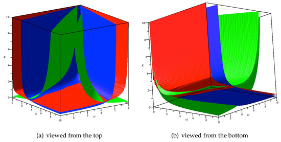
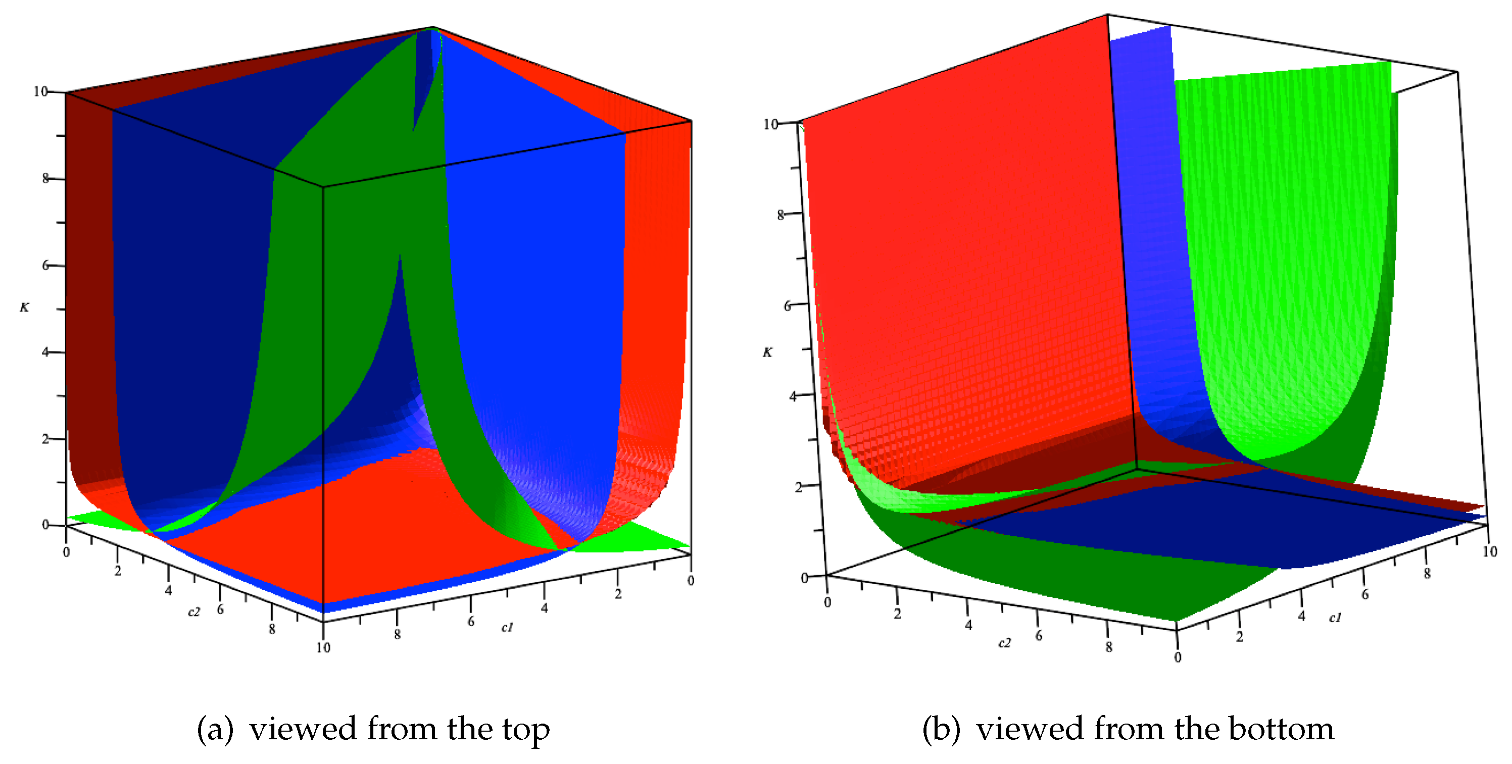
Then the stability condition of our model is simply $N<0$. In Figure 1, we depict the surfaces of $N=0$, $L_1=0$ and $L_2=0$ in red, blue and green, respectively, using the $implicitplot3d$ function in Maple 2022.

Figure 1. The 3-dimensional $(c_1,c_2,K)$ parameter space. The red, blue and green surfaces are $N=0$, $L_1=0$ and $L_2=0$, respectively.

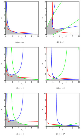
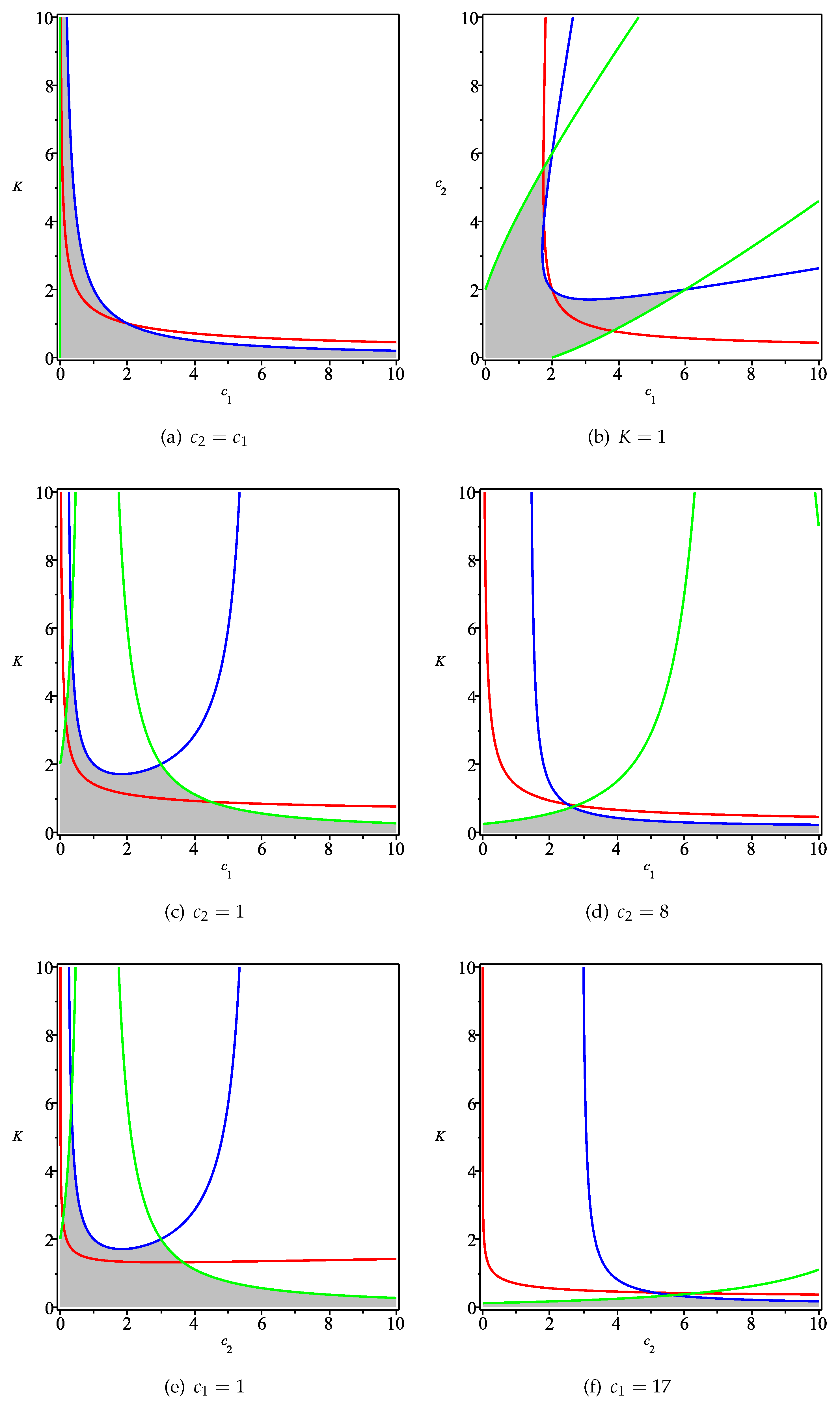
Furthermore, Figure 2 depicts several 2-dimensional subspaces of parameter values with one parameter fixed. The curves corresponding to $N=0$, $L_1=0$ and $L_2=0$ are marked in red, blue and green, respectively. For each subfigure of Figure 2, our model is locally stable in the region surrounded by the red line and the two axes, while the stability region of its analogue under linear costs is colored in grey. The $implicitplot3d$ function only gives us an approximate view of the three surfaces, but some places in Figure 1 seem inaccurate, e.g., the region around the origin $(0,0,0)$. If $c_2=c_1$, then $L_1=0$ is transformed to $c_1=0$, i.e., the vertical axis in Figure 2a, which is not precisely captured by Figure 1. As shown by Figure 2a, given $c_2=c_1$, it is always possible to find a combination of the parameters $c_1$ and K such that our Cournot–Nash equilibrium $E_1$ and the equilibrium of Tramontana’s are

• Both locally stable;
• Both locally unstable;
• One locally stable and the other locally unstable.

From Figure 2b,c, similar features as above can be observed. Figure 2b depicts the special case of the unit speed of adjusting the first firm’s output, i.e., $K=1$. In addition, the other two cases where the second firm has a small ($c_2=1$) and a large ($c_2=8$) cost parameter are shown in (c) and (d), respectively. In general, from all the subfigures in Figure 2, it is observed that a reduction in the cost parameter ($c_1$ or $c_2$) has an effect of enhancing the local stability for both our model and Tramontana’s. Furthermore, both models would be destabilized if the speed parameter K of adjustment becomes large enough.

Figure 2. The 2-dimensional subspaces of the parameter values with one parameter fixed. The curves corresponding to $N=0$, $L_1=0$ and $L_2=0$ are marked in red, blue and green, respectively. For each case, the model considered in this paper is locally stable in the region surrounded by the red line and the two axes; the analogue under linear costs is locally stable in the grey region that is surrounded by the blue, the green lines and the two axes.

Figure 2. The 2-dimensional subspaces of the parameter values with one parameter fixed. The curves corresponding to $N=0$, $L_1=0$ and $L_2=0$ are marked in red, blue and green, respectively. For each case, the model considered in this paper is locally stable in the region surrounded by the red line and the two axes; the analogue under linear costs is locally stable in the grey region that is surrounded by the blue, the green lines and the two axes.

The comparison between Figure 2c,d (or Figure 2e,f) is quite informative. In (c) or (e), the stability region of Tramontana’s model is not covered by our model and vice versa. However, in (d) or (f), it seems that the stability region of Tramontana’s model is strictly contained in that of our model. Consequently, we conjecture that if $c_2$ or $c_1$ is large enough, the stability region of our model is strictly larger than that of Tramontana’s. We use the symbolic computation to formally prove this conjecture in Corollary 1.

Corollary 1.

The stability region of map (3) covers that of its analogue under linear costs provided that $c_1>{(19/10)}^4$ or $c_2>{(17/10)}^4$.

Proof. 

We need to prove that (9) is true if both (12) and (13) are satisfied. This may be extremely difficult to acquire through a manually mathematical derivation. However, we provide another proof in a computational style. Denote $a=\sqrt[4]{c_1}$ and $b=\sqrt[4]{c_2}$. Then (9) is equivalent to

$$C{D}_1<0:K\left(\sqrt{2}{a}^{3}b\left(a^4+6a^2{b}^2+b^4\right)\right)-{\left(a^2+b^2\right)}^2\left(3a^2+b^2\right)<0,$$

while (12) and (13) are transformed into

$$C{D}_2<0:K(4a^4{b}^4-{(b^4-a^4)}^2)-4(a^4+b^4)<0,$$

and

$$C{D}_3<0:K{(b^4-a^4)}^2-2(a^4+b^4)<0,$$

respectively. Obviously, the set $\left\{\right(a,b,K\left)\right|a>19/10,b>0,K>0\}$ for $c_1>{(19/10)}^4$ and the set $\left\{\right(a,b,K\left)\right|a,b>17/10,K>0\}$ for $c_2>{(17/10)}^4$ are of our concern.

The main idea of our computational proof is as follows. $C{D}_1=0$, $C{D}_2=0$ and $C{D}_3=0$ divide $\left\{\right(a,b,K\left)\right|a>19/10,b>0,K>0\}$ or $\left\{\right(a,b,K\left)\right|a,b>17/10,K>0\}$ into a number of regions. In a fixed region, the signs of $C{D}_1$, $C{D}_2$ and $C{D}_3$ are invariant. Therefore, we only need to select one sample point from each region, and then determine the signs of $C{D}_1$, $C{D}_2$ and $C{D}_3$ at these selected sample points. If at all the sample points where $C{D}_1<0$ and $C{D}_2<0$ are satisfied $C{D}_3<0$ is also true, then it can be concluded that $C{D}_1<0$ and $C{D}_2<0$ implies $C{D}_3<0$.

For simple cases, sample points could be easily selected. However, in general, the selection might be extremely complicated and could be automated using, e.g., the partial cylindrical algebraic decomposition (PCAD) method [24]. For the case of $c_1>{(19/10)}^4$, the PCAD method permits us to select 44 sample points from the set $\left\{\right(a,b,K\left)\right|a>19/10,b>0,K>0\}$, which are all listed in Table 1. It is observed from Table 1 that at all the sample points where both $C{D}_1<0$ and $C{D}_2<0$ are true, $C{D}_3<0$ is also true. For the case of $c_2>{(17/10)}^4$, we consider $\left\{\right(a,b,K\left)\right|a,b>17/10,K>0\}$, where 359 sample points are selected by our implementation. We do not give the corresponding table due to the space limitation, but our calculations show that $C{D}_1<0$ and $C{D}_2<0$ also imply $C{D}_3<0$. It should be noted that all the involved computations are symbolic instead of numerical, which means the obtained results are precise and imply the correctness of this corollary. □

Table 1. Selected Sample Points for $\left\{\right(a,b,K\left)\right|a>19/10,b>0,K>0\}$.

Sample Point of $(\mathit{a},\mathit{b},\mathit{K})$	${\mathit{CD}}_1<0$	${\mathit{CD}}_2<0$	${\mathit{CD}}_3<0$
$(a=77/32,b=89/128,K=31/1024)$	true	true	true
$(a=77/32,b=89/128,K=2189/4096)$	true	false	true
$(a=77/32,b=89/128,K=97/64)$	true	false	false
$(a=77/32,b=377/256,K=47/1024)$	true	true	true
$(a=77/32,b=377/256,K=479/2048)$	true	false	true
$(a=77/32,b=377/256,K=225/256)$	true	false	false
$(a=77/32,b=209/128,K=119/2048)$	true	true	true
$(a=77/32,b=209/128,K=115/512)$	true	false	true
$(a=77/32,b=209/128,K=31/64)$	true	false	false
$(a=77/32,b=209/128,K=73/64)$	false	false	false
$(a=77/32,b=227/128,K=79/1024)$	true	true	true
$(a=77/32,b=227/128,K=195/1024)$	true	false	true
$(a=77/32,b=227/128,K=17/64)$	false	false	true
$(a=77/32,b=227/128,K=207/256)$	false	false	false
$(a=77/32,b=243/128,K=9/128)$	true	true	true
$(a=77/32,b=243/128,K=185/1024)$	false	true	true
$(a=77/32,b=243/128,K=259/1024)$	false	false	true
$(a=77/32,b=243/128,K=101/128)$	false	false	false
$(a=77/32,b=35/16,K=39/1024)$	true	true	true
$(a=77/32,b=35/16,K=343/2048)$	false	true	true
$(a=77/32,b=35/16,K=321/512)$	false	true	false
$(a=77/32,b=35/16,K=3/2)$	false	false	false
$(a=77/32,b=667/256,K=27/1024)$	true	true	true
$(a=77/32,b=667/256,K=589/4096)$	false	true	true
$(a=77/32,b=667/256,K=637/1024)$	false	true	false
$(a=77/32,b=667/256,K=97/64)$	false	false	false
$(a=77/32,b=765/256,K=27/1024)$	true	true	true
$(a=77/32,b=765/256,K=325/4096)$	false	true	true
$(a=77/32,b=765/256,K=343/2048)$	false	false	true
$(a=77/32,b=765/256,K=187/256)$	false	false	false
$(a=77/32,b=435/128,K=17/1024)$	true	true	true
$(a=77/32,b=435/128,K=241/4096)$	true	false	true
$(a=77/32,b=435/128,K=321/2048)$	false	false	true
$(a=77/32,b=435/128,K=187/256)$	false	false	false
$(a=77/32,b=943/256,K=39/4096)$	true	true	true
$(a=77/32,b=943/256,K=1023/8192)$	true	false	true
$(a=77/32,b=943/256,K=339/1024)$	true	false	false
$(a=77/32,b=943/256,K=239/256)$	false	false	false
$(a=77/32,b=969/256,K=33/4096)$	true	true	true
$(a=77/32,b=969/256,K=1019/8192)$	true	false	true
$(a=77/32,b=969/256,K=47/64)$	true	false	false
$(a=77/32,b=555/128,K=123/\mathrm{32,768})$	true	true	true
$(a=77/32,b=555/128,K=1039/8192)$	true	false	true
$(a=77/32,b=555/128,K=383/512)$	true	false	false

Remark 1.

It is difficult but meaningful to find the necessary and sufficient condition that the stability region of our model covers that of its analogue. However, we should mention that Corollary 1 is close to this necessary and sufficient condition because it can be proved by the symbolic computation that Corollary 1 would be false if the condition is replaced with $c_1>{(18/10)}^4$ or $c_2>{(16/10)}^4$.

For example, if we set

$$c_1={\left(\frac{469}{256}\right)}^4\approx 1.{832}^4,c_2={\left(\frac{711}{512}\right)}^4\approx 1.{389}^4,K=\frac{133}{256}\approx 0.520,$$

which satisfies that $c_1>{(18/10)}^4$, then one can verify that

$$\begin{array}{cc}\hfill C{D}_1& =\frac{19732367954412426944060794575906178572080970918849}{22835963083295358096932575511191922182123945984}>0,\hfill \\ \hfill C{D}_2& =-\frac{2978317644286814417291621}{1208925819614629174706176}<0,\hfill \\ \hfill C{D}_3& =-\frac{462313018677420397986139}{1208925819614629174706176}<0.\hfill \end{array}$$

In this case, we know both $C{D}_1<0$ and $C{D}_2<0$ are true does not imply that $C{D}_3<0$ is true.

Moreover, if we set

$$c_1={\left(\frac{4973}{4096}\right)}^4\approx 1.{214}^4,c_2={\left(\frac{3279}{2048}\right)}^4\approx 1.{601}^4,K=\frac{115}{128}\approx 0.898,$$

which satisfies that $c_2>{(16/10)}^4$, then we can verify that

$$\begin{array}{cc}\hfill C{D}_1& =\frac{1473408087700784653120374786339483004819598680136381150500196337}{25711008708143844408671393477458601640355247900524685364822016}>0,\hfill \\ \hfill C{D}_2& =-\frac{10587335994218834247243889619379}{10141204801825835211973625643008}<0,\hfill \\ \hfill C{D}_3& =-\frac{1090191459559314074736442742157}{10141204801825835211973625643008}<0.\hfill \end{array}$$

According to Corollary 1, diseconomies of scale stabilize the heterogeneous duopoly game with a boundedly rational player and a naive player if the cost parameters are large enough. This conclusion is consistent with the result by Fisher [2] as well as that by McManus and Quand [16], that increasing marginal cost is a stabilizing influence for homogeneous oligopolies under linear demand. We should mention that the studies of [2,16] considered only homogeneous mechanisms of adjusting firms’ outputs and a linear demand function, but we introduce heterogeneous players and a nonlinear demand to our study. In contrast, Dubiel-Teleszynski [3] discovered that industries facing diseconomies of scale are less stable than those facing constant marginal costs, which is different from our findings.

4. Numerical Simulations

In this section, through numerical simulations, we demonstrate that the dynamic behavior of a duopoly game in face of diseconomies of scale could be greatly distinct from its analogue under constant return to scale. Our model would lose its local stability through a period-doubling bifurcation ($P(-1)=0$). Meanwhile, two possible routes to complicated dynamics exist for its analogue: a cascade of period-doubling bifurcations and a Neimark–Sacker bifurcation. In the sequel, we keep the two cost parameters $c_1$ and $c_2$ fixed at $(c_1,c_2)=(0.5,1.0)$ and vary the adjustment speed K of the first firm. Moreover, the initial state of the iteration map (3) is assumed to be $\left(x\right(0),y(0\left)\right)=(0.5,0.5)$ in our numerical simulations.

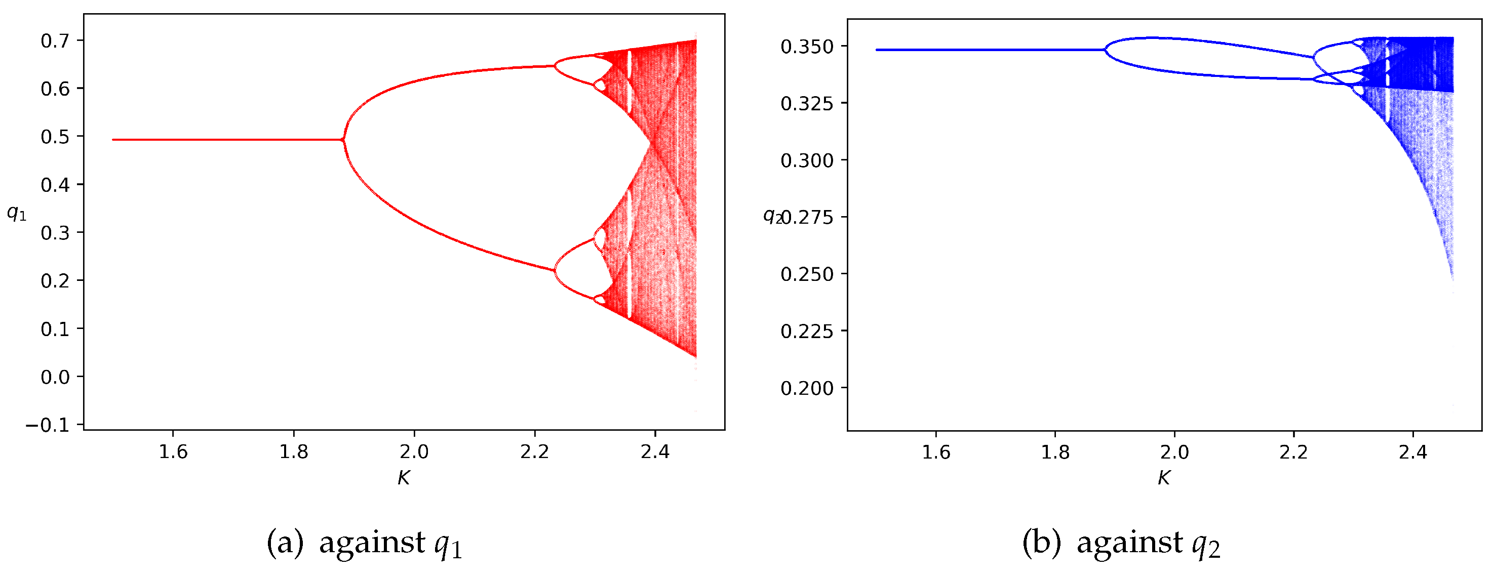
Figure 3 depicts the bifurcation diagrams against $q_1$ and $q_2$ concerning K, which shows the dynamic behavior in the region of stability and the period-doubling route to chaos. An increase in the adjustment speed K has a destabilizing effect if keeping other parameters fixed. Recalling Figure 2c, one can see that an increase of K brings the point upwards along the line $c_1=1/2$, then crossing the period-doubling bifurcation curve (the red one), and finally out of the region of stability.

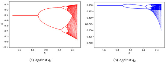
Figure 3. The bifurcation diagrams of the iteration map (3) with respect to K if fixing the parameters $c_1=0.5$, $c_2=1.0$ and setting the initial state as $\left(x\right(0),y(0\left)\right)=(0.5,0.5)$. The bifurcation diagrams against $q_1$ is given in (a), and that against $q_2$ is given in (b).

As shown in Figure 3, the unique equilibrium $E_1\approx (0.493,0.348)$ is locally stable if K is less than $1.884$. Afterward, a cascade of period-doubling bifurcations leading to periodic cycles, which is most common in dynamic economic models, can be observed. In particular, stable period-2 orbits occur when $K\in (1.884,2.233)$, and stable period-4 orbits arise when $K\in (2.233,2.297)$, which are followed by periodic orbits of higher orders. From an economic point of view, it is quite realistic to assume that boundedly rational firms cannot learn the pattern behind quantities and profits if long periodic dynamics take place.

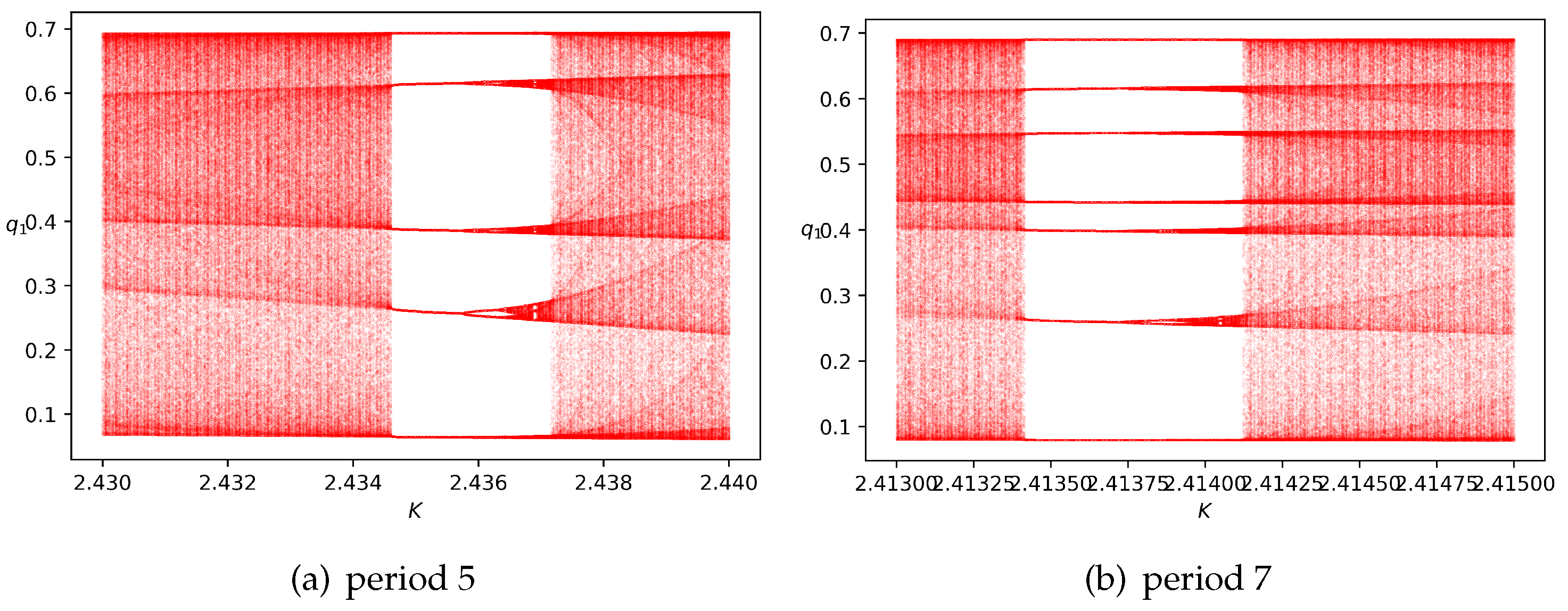
As K increases from $2.316$, our model starts to undergo chaotic dynamics. If chaos appears, the pattern behind productions and profits is nearly impossible to learn, even for completely rational players. It is known that chaotic attractors are fractal sets since at small scales a chaotic attractor is approximately the Cartesian product of a Cantor set and a line segment; thus it is roughly self-similar and has a box dimension that is not an integer. Fractal patterns are quite common as nature is full of fractals. Herein, it is discovered that fractal patterns are also widespread in economic systems. Moreover, at some values of K greater than $2.316$, periodic solutions of odd orders (see Figure 4 for period 5 and period 7) could be discovered. We also observe other periods, e.g., 6, 10 and 20, through our numerical simulations.

Figure 4. Periodic orbits of odd orders found in the bifurcation diagrams of the iteration map (3) with respect to K against $q_1$ if fixing the parameters $c_1=0.5$, $c_2=1.0$ and setting the initial state as $\left(x\right(0),y(0\left)\right)=(0.5,0.5)$. An orbit of period 5 can be observed in (a), and an orbit of period 7 can be observed in (b).

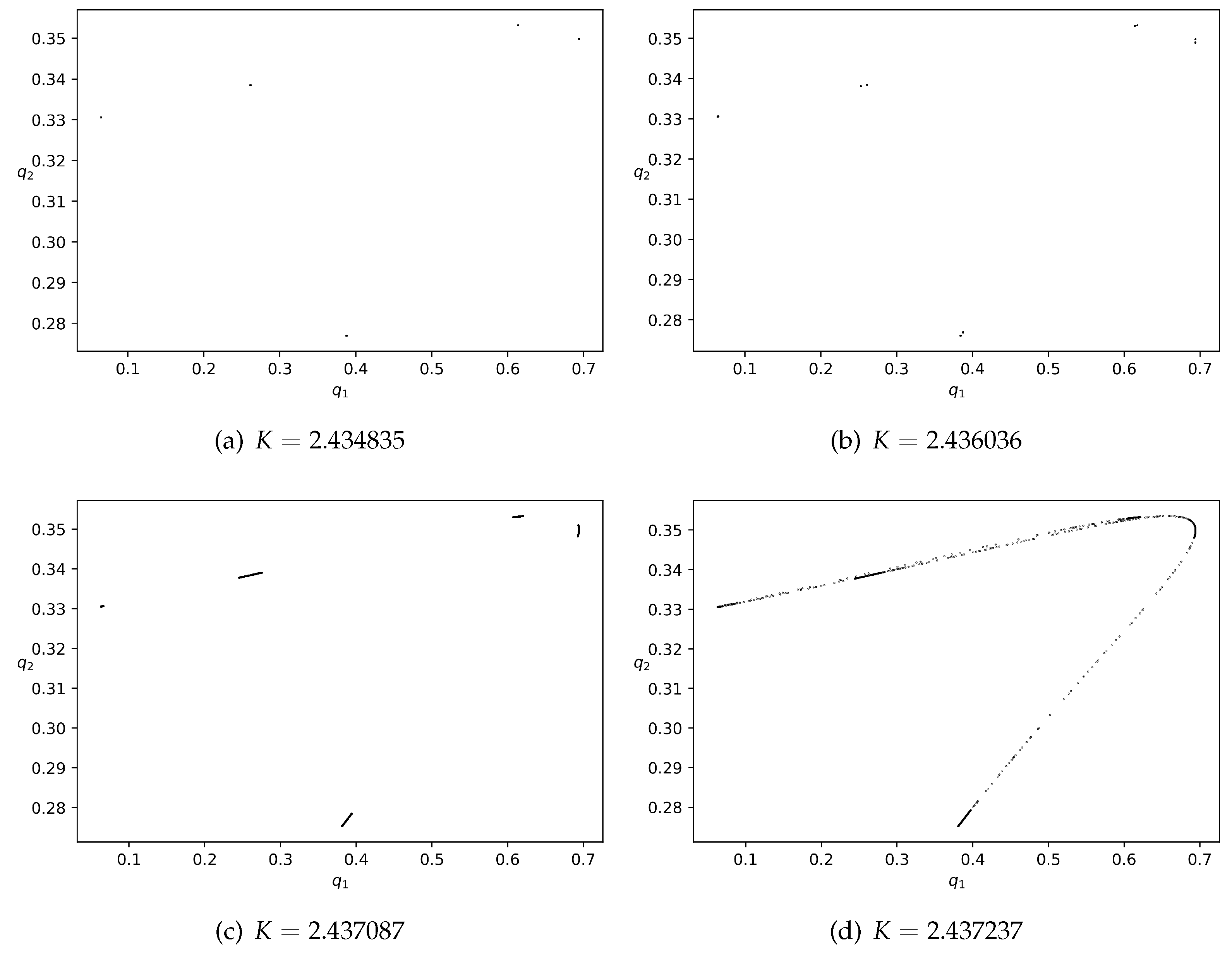
Figure 5 shows phase portraits corresponding to four different values of K with the other parameters fixed and demonstrates the evolution of dynamics after the appearance of period 5 (also see Figure 4a). After an interval of chaos, periodic solutions of period 5 (see Figure 5a) arise in our model. As the value of K increases, we can also observe a cascade of period-doubling bifurcations inside the periodic window. In particular, Figure 5b depicts the orbit of period 10 after a bifurcation. After that, cyclical chaotic areas can be found (see the five dark pieces in Figure 5c), which is followed by one piece of the strange attractor (see Figure 5d). Moreover, it seems that the areas around the original positions of the periodic orbit are darker in Figure 5d; that is, points nearby the original periodic orbit are more frequently visited even as chaotic dynamics take place.

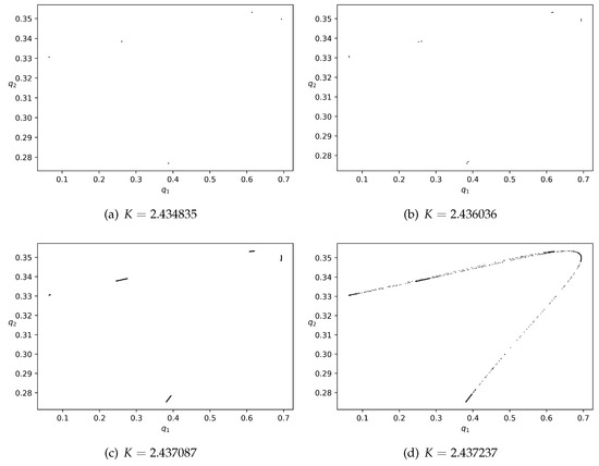
Figure 5. The phase portraits if fixing the parameters $c_1=0.5$, $c_2=1.0$ and setting the initial state as $\left(x\right(0),y(0\left)\right)=(0.5,0.5)$.

5. Concluding Remarks

In this paper, we investigated the local stability and the bifurcation of a heterogeneous duopoly model under the assumptions of an isoelastic demand and quadratic costs. The nonlinearity of firms’ costs permits us to extend the applications of the standard Cournot model to oligopolistic markets in face of diseconomies of scale. In our model, two firms have different decision mechanisms: one is a boundedly rational player that adopts a gradient adjusting mechanism; the other is a naive player that has a naive expectation of its rival’s production plan.

Our work primarily studied how diseconomies of scale affect the dynamic behavior of a heterogeneous duopoly game under an isoelastic demand. If the cost parameters are large enough, we found that diseconomies of scale can stabilize the model, which is consistent with the result by Fisher [2] as well as that by McManus and Quandt [16]. It should be mentioned that the studies of [2,16] considered only homogeneous mechanisms of adjusting firms’ outputs and a linear demand function. However, we introduced heterogeneous agents and a nonlinear demand to our investigation. Furthermore, we unveiled another crucial difference between our model and its analogue by Tramontana [13]: our model loses its local stability through a period-doubling bifurcation, but its analogue could be destabilized through two possible routes, i.e., through a period-doubling bifurcation and a Neimark–Sacker bifurcation.

The investigation of oligopoly models becomes complicated when the market demand is nonlinear, and the costs are also nonlinear. To the best of our knowledge, under the assumptions of an isoelastic demand and quadratic costs, no homogeneous oligopoly models with boundedly rational players or with naive players have been discussed in the current literature. We leave these models for future research.

References

- Cournot, A.A. Recherches sur les Principes Mathématiques de la Théorie des Richesses; L. Hachette: Paris, France, 1838. [Google Scholar]
- Fisher, F.M. The stability of the Cournot oligopoly solution: The effects of speeds of adjustment and increasing marginal costs. Rev. Econ. Stud. 1961, 28, 125. [Google Scholar] [CrossRef]
- Dubiel-Teleszynski, T. Nonlinear dynamics in a heterogeneous duopoly game with adjusting players and diseconomies of scale. Commun. Nonlinear Sci. Numer. Simul. 2011, 16, 296–308. [Google Scholar] [CrossRef]
- Puu, T. Chaos in duopoly pricing. Chaos Solitons Fractals 1991, 1, 573–581. [Google Scholar] [CrossRef]
- Bischi, G.I.; Naimzada, A.; Sbragia, L. Oligopoly games with local monopolistic approximation. J. Econ. Behav. Organ. 2007, 62, 371–388. [Google Scholar]
- Ahmed, E.; Agiza, H.; Hassan, S. On modifications of Puu’s dynamical duopoly. Chaos Solitons Fractals 2000, 11, 1025–1028. [Google Scholar] [CrossRef]
- Cavalli, F.; Naimzada, A.; Tramontana, F. Nonlinear dynamics and global analysis of a heterogeneous Cournot duopoly with a local monopolistic approach versus a gradient rule with endogenous reactivity. Commun. Nonlinear Sci. Numer. Simul. 2015, 23, 245–262. [Google Scholar] [CrossRef] [Green Version]
- Askar, S.S.; Alnowibet, K. Nonlinear oligopolistic game with isoelastic demand function: Rationality and local monopolistic approximation. Chaos Solitons Fractals 2016, 84, 15–22. [Google Scholar] [CrossRef]
- Elsadany, A.A. Dynamics of a Cournot duopoly game with bounded rationality based on relative profit maximization. Appl. Math. Comput. 2017, 294, 253–263. [Google Scholar] [CrossRef]
- Kopel, M. Simple and complex adjustment dynamics in Cournot duopoly models. Chaos Solitons Fractals 1996, 7, 2031–2048. [Google Scholar]
- Li, B.; Liang, H.; Shi, L.; He, Q. Complex dynamics of Kopel model with nonsymmetric response between oligopolists. Chaos Solitons Fractals 2022, 156, 111860. [Google Scholar] [CrossRef]
- Naimzada, A.; Tramontana, F. Controlling chaos through local knowledge. Chaos Solitons Fractals 2009, 42, 2439–2449. [Google Scholar] [CrossRef] [Green Version]
- Tramontana, F. Heterogeneous duopoly with isoelastic demand function. Econ. Model. 2010, 27, 350–357. [Google Scholar] [CrossRef]
- Bischi, G.I.; Kopel, M.; Szidarovszky, F. Expectation-stock dynamics in multi-agent fisheries. Ann. Oper. Res. 2005, 137, 299–329. [Google Scholar] [CrossRef]
- Li, X.; Wang, D. Computing equilibria of semi-algebraic economies using triangular decomposition and real solution classification. J. Math. Econ. 2014, 54, 48–58. [Google Scholar] [CrossRef] [Green Version]
- McManus, M.; Quandt, R.E. Comments on the stability of the Cournot oligipoly model. Rev. Econ. Stud. 1961, 28, 136–139. [Google Scholar] [CrossRef]
- Agiza, H.N.; Elsadany, A.A. Chaotic dynamics in nonlinear duopoly game with heterogeneous players. Appl. Math. Comput. 2004, 149, 843–860. [Google Scholar] [CrossRef]
- Wu, W.T. Basic principles of mechanical theorem proving in elementary geometries. J. Autom. Reason. 1986, 2, 221–252. [Google Scholar]
- Kalkbrener, M. A generalized Euclidean algorithm for computing triangular representations of algebraic varieties. J. Symb. Comput. 1993, 15, 143–167. [Google Scholar] [CrossRef] [Green Version]
- Aubry, P.; Moreno Maza, M. Triangular sets for solving polynomial systems: A comparative implementation of four methods. J. Symb. Comput. 1999, 28, 125–154. [Google Scholar]
- Wang, D. Computing triangular systems and regular systems. J. Symb. Comput. 2000, 30, 221–236. [Google Scholar] [CrossRef]
- Li, X.; Mou, C.; Wang, D. Decomposing polynomial sets into simple sets over finite fields: The zero-dimensional case. Comput. Math. Appl. 2010, 60, 2983–2997. [Google Scholar] [CrossRef]
- Jury, E.; Stark, L.; Krishnan, V. Inners and stability of dynamic systems. IEEE Trans. Syst. Man Cybern. 1976, 10, 724–725. [Google Scholar] [CrossRef]
- Collins, G.E.; Hong, H. Partial cylindrical algebraic decomposition for quantifier elimination. J. Symb. Comput. 1991, 12, 299–328. [Google Scholar] [CrossRef] [Green Version]
Publisher’s Note: MDPI stays neutral with regard to jurisdictional claims in published maps and institutional affiliations. |
© 2022 by the authors. Licensee MDPI, Basel, Switzerland. This article is an open access article distributed under the terms and conditions of the Creative Commons Attribution (CC BY) license (https://creativecommons.org/licenses/by/4.0/).