An Energy Conserving Numerical Scheme for the Klein–Gordon Equation with Cubic Nonlinearity

Abstract

In this paper, we develop a numerical scheme that conserves the discrete energy for solving the Klein-Gordon equation with cubic nonlinearity. We prove theoretically that our scheme conserves not just discrete energy, but also other energy-like discrete quantities. In addition, we prove the convergence and the stability of the scheme. Finally, we present some numerical simulations to demonstrate the performance of our energy-conserving scheme.

1. Introduction

The Klein–Gordon equation is a well-studied equation in mathematical physics in terms of radiation theory, nonlinear optics and general relativity of scattering [1,2,3]. In particular, much work has been carried out on the Klein–Gordon equation with respect to wave collisions and resonance behavior [4]. Recently, we considered the Klein–Gordon equation with quintic nonlinearity from the analytical point of view and were able to obtain a number of new wave solutions [5]. In this paper, our focus is on the numerical study of the initial value problem of the Klein–Gordon equation with cubic nonlinearity

$$\begin{array}{ccc}\hfill u_{tt}-u_{xx}=\alpha u-\beta u^3,& -\infty <x<\infty ,& t\ge 0,\hfill \end{array}$$

(1)

with the initial conditions

$$\begin{array}{ccc}\hfill u(x,0)=u_0\left(x\right),& u_t(x,0)=u_1\left(x\right),& -\infty <x<\infty ,\hfill \end{array}$$

where $\alpha$ and $\beta$ are arbitrary positive constants, and $u_0\left(x\right)$ and $u_1\left(x\right)$ are known smooth functions. Here, one should note that the non-local version of $\left(1\right)$, where the dependence of previous time history is considered, gives a time-fractional nonlinear Klein–Gordon equation [6]. There have been a number of analytical and numerical studies to understand the solutions of nonlinear time and space-fractional Klein–Gordon equations [7,8,9,10,11]. The numerical studies have focused on various techniques to discretize the fractional derivatives. However, no special attention was given to the nonlinearities in the equations, as we do in Section 2.

In order to construct a numerical scheme for solving $\left(1\right)$, we re-cast the initial value problem as the following initial boundary value problem:

$$\begin{array}{ccc}\hfill u_{tt}-u_{xx}=\alpha u-\beta u^3,& x_L\le x\le x_R,& 0\le t<T,\hfill \end{array}$$

(2)

with the initial conditions

$$\begin{array}{ccc}\hfill u(x,0)=u_0\left(x\right),& u_t(x,0)=u_1\left(x\right),& x_L\le x\le x_R,\hfill \end{array}$$

(3)

and the boundary conditions

$$\begin{array}{ccc}\hfill u(x_L,t)=0,& u(x_R,t)=0,& 0\le t\le T.\hfill \end{array}$$

(4)

Here $x_L$ is negative, and $x_R$ is positive with $\left|x_L\right|$ and $x_R$ being large values so that the finite spatial domain $x_L\le x\le x_R$ mimics the infinite domain $-\infty <x<\infty$. Moreover, T can be large. In some cases, the boundary conditions $\left(4\right)$ may be replaced by

$$\begin{array}{ccc}\hfill u(x_L,t)=\mp \sqrt{\frac{\alpha }{\beta }},& u(x_R,t)=\pm \sqrt{\frac{\alpha }{\beta }},& 0\le t\le T.\hfill \end{array}$$

The boundary conditions at $u(x_L,t)$ and $u(x_R,t)$ for the problem $\left(2\right)$ correspond to the asymptotic conditions for $u(x,t)$ of $\left(1\right)$ as x goes to $-\infty$ and ∞. The solution $u(x,t)$ of the initial boundary value problem $\left(2\right)$–$\left(4\right)$ formally satisfies the following energy identity:

$$E=\underset{x_L}{\overset{x_R}{\int }}\left[{\left({\partial }_{t}u\right)}^2+{\left({\partial }_{x}u\right)}^2-\alpha u^2+\frac{\beta }{2}{u}^4\right]dx=\mathrm{const}.$$

(5)

In the literature, one can find a number of numerical schemes with conservation properties for solving the nonlinear Klein–Gordon equation. For example, a three-level finite difference method that conserves energy was developed in [12], while other finite-difference algorithms that preserve energy or linear momentum were studied in [13]. In addition, there are schemes that were constructed using a variational iteration method [14,15], a homotopy-perturbation idea [16,17], radial basis functions [18], spline-collocation approach [19] and discrete Fourier transforms [20] to solve the Klein–Gordon equation under various conditions. Further, some of the recent studies on the nonlinear Klein–Gordon equation have involved making use of pseudo-spectral discretization methods [21], employing a differential quadrature method with cubic B-splines [22] and domain decomposition methods [23]. Other studies include making use of the sinc-collocation idea along with a discrete gradient method to study the Klein–Gordon–Schrödinger equation [24] and developing a higher order method for the Klein–Gordon equation employing a local discontinuous Galerkin method [25]. However, in [25], the numerical simulations were carried out only for the linear Klein–Gordon equation. In [26], energy-preserving schemes were constructed for higher dimensional Klein–Gordon equations using the discrete gradient method and Duhamel principle. In addition, there have been a couple of interesting analytical studies of the Klein–Gordon equation, one utilizing an operational matrix method with clique polynomials [27] and the other a series method using differential transforms [28].

Most of the existing numerical methods investigate the conservation of discrete energy only numerically. If one is to validate the numerical results of an energy conserving numerical scheme, it is important to prove theoretically that the scheme conserves the discrete energy. The work in [29] carried out a theoretical study of four explicit finite difference schemes for solving the Klein–Gordon equation. In the spirit of [29], this paper presents an implicit conservative finite difference scheme for the initial boundary value problem $\left(2\right)$–$\left(4\right)$. It should be noted that in [30] implicit finite difference schemes were studied for the coupled system of Klein–Gordon–Zakharov equations. Later, more work along the same lines was conducted in [31] for the same system. Even though there is some similarity, in contrast to those works, our study considers not just the conservation of the discrete energy, but other energy-like discrete quantities as well. A predictor–corrector idea is employed to deal with the nonlinearity which appears in the problem. Furthermore, we give some a priori estimates and then prove by the discrete energy method that the difference scheme is stable and second-order convergent. Some numerical results are presented to illustrate the theoretical results. Three-dimensional plots are displayed to demonstrate the sensitivity of the discrete energy and other discrete quantities to the choices of time steps, wave speed, and coefficients $\alpha$ and $\beta$.

2. Finite Difference Scheme and Its Conservation Law

Before we propose the conservative finite difference scheme for the Klein–Gordon equation with cubic nonlinearity $\left(2\right)$–$\left(4\right)$, we give some notations as follows when we discretize the space and time domains:

$$\begin{array}{cc}\hfill x_m=x_L+mh,& 0\le m\le M=\left[\frac{x_R-x_L}{h}\right],\end{array}$$

$$\begin{array}{cc}\hfill t^n=n\tau ,& n=0,1,2,\dots ,N=\left[\frac{T}{\tau }\right],\end{array}$$

$$\begin{array}{cc}\hfill {\left(w_m^n\right)}_x={\displaystyle \frac{w_{m+1}^n-w_m^n}{h}},& {\left(w_m^n\right)}_{\overline{x}}={\displaystyle \frac{w_m^n-w_{m-1}^n}{h}},\end{array}$$

$$\begin{array}{cc}\hfill {\left(w_m^n\right)}_t={\displaystyle \frac{w_m^{n+1}-w_m^n}{\tau }},& {\left(w_m^n\right)}_{\overline{t}}={\displaystyle \frac{w_m^n-w_m^{n-1}}{\tau }},\end{array}$$

where h and $\tau$ are the step sizes of space and time, respectively. In addition, we define the following inner product and norms:

$$\begin{array}{ccc}\hfill ⟨w^n,u^n⟩=h{\displaystyle \sum _{m=0}^M}{w}_m^n{u}_m^n,& & {∥w^n∥}_p^p=h{\displaystyle \sum _{m=0}^M}{\left|w_m^n\right|}^p,\hfill \end{array}$$

${∥w^n∥}_{\infty }={sup}_{0\le m\le M}\left|w_m^n\right|.$

It should be noted that in the following, C stands for a general positive constant that may take different values on different occasions. In addition, for brevity, we omit the subscript 2 of ${∥w^n∥}_2$.

Lemma 1.

For any two mesh functions $\left\{w_m\right\}$ and $\left\{v_m\right\},$ $m=0,1,2,\dots ,M,$ there is the identity

$$h\sum _{m=0}^{M-1}{w}_m{\left(v_m\right)}_{x\overline{x}}=-h\sum _{m=0}^{M-1}{\left(w_m\right)}_x{\left(v_m\right)}_x-w_0{\left(v_0\right)}_x+w_M{\left(v_M\right)}_{\overline{x}}.$$

This lemma can be easily proved using the notational definitions directly.

Let $U_m^n$ be the difference approximation of $u(x,t)$ at $(x_m,t^n);$ that is, $U_m^n\approx u(x_m,t^n).$ In addition, assume that $u_0\left(x_m\right)=U_0\left(x_m\right)$ and $u_1\left(x_m\right)=U_1\left(x_m\right).$

Now, we consider the following finite difference scheme for the Klein–Gordon equation with cubic nonlinearity $\left(2\right)$–$\left(4\right)$:

$$\begin{array}{cc}\hfill {\left(U_m^n\right)}_{t\overline{t}}-\frac{1}{2}{\left(U_m^{n+1}+U_m^{n-1}\right)}_{x\overline{x}}& -\frac{\alpha }{2}\left(U_m^{n+1}+U_m^{n-1}\right)\hfill \\ & +\frac{\beta }{4}\left(U_m^{n+1}+U_m^{n-1}\right)\left({\left(U_m^{n+1}\right)}^2+{\left(U_m^{n-1}\right)}^2\right)=0.\hfill \end{array}$$

(6)

In order to employ the finite difference scheme $\left(6\right)$, we need initial values at two different time levels. They are chosen from the initial conditions given in $\left(3\right)$ such that

$$\begin{array}{c}\hfill U_m^0=U_0\left(x_m\right)\mathrm{and}\frac{U_m^1-U_m^{-1}}{2\tau }=U_1\left(x_m\right)\end{array}$$

(7)

making use of a fictitious time level $-1$.

The boundary conditions are as below.

$$\begin{array}{cc}\hfill U_0^n=0,& U_M^n=0.\end{array}$$

(8)

It should be pointed out that our two-time-level split approximation of the nonlinear cubic term is very different than the standard nonlinear approximation. As will be seen later in Theorems 1 and 2, this split approximation makes the theoretical analysis easier.

In $\left(6\right)$, the explicit forms of ${\left(U_m^n\right)}_{t\overline{t}}$ and ${\left(U_m^n\right)}_{x\overline{x}}$ are given as follows:

$$\begin{array}{cc}\hfill {\left(U_m^n\right)}_{t\overline{t}}={\displaystyle \frac{U_m^{n+1}-2U_m^n+U_m^{n-1}}{{\tau }^2}},& {\left(U_m^n\right)}_{x\overline{x}}={\displaystyle \frac{U_{m+1}^n-2U_m^n+U_{m-1}^n}{h^2}}.\end{array}$$

As noted before, the solution $u(x,t)$ of the initial boundary-value problem $\left(2\right)$–$\left(4\right)$ satisfies the following energy identity:

$$E=\underset{x_L}{\overset{x_R}{\int }}\left[{\left({\partial }_{t}u\right)}^2+{\left({\partial }_{x}u\right)}^2-\alpha u^2+\frac{\beta }{2}{u}^4\right]dx=\mathrm{const}.$$

Now, we present some properties of our finite difference scheme.

Theorem 1.

The difference scheme $\left(6\right)$–$\left(8\right)$ possesses the following property:

$$Q^n=Q^{n-1}+\mathcal{O}\left(h\tau \right),$$

(9)

where

$$Q^n={∥U_t^n∥}^2+\frac{1}{2}{∥U_x^n∥}^2-\frac{\alpha }{2}{∥U^n∥}^2+\frac{\beta }{4}{∥U^n∥}_4^4.$$

(10)

Proof. 

Computing the inner product of $\left(6\right)$ with $U^n-U^{n-1}$, we have

$$\begin{array}{c}{∥U_t^n∥}^2-{∥U_t^{n-1}∥}^2-h{\displaystyle \sum _{m=0}^M}\frac{1}{{\tau }^2}\left[U_m^{n+1}-2U_m^n+U_m^{n-1}\right]\left[U_m^{n+1}-U_m^{n-1}\right]\hfill \\ \hfill +\frac{1}{2}\left({∥U_x^n∥}^2-{∥U_x^{n-1}∥}^2\right)-\frac{\alpha }{2}\left({∥U^n∥}^2-{∥U^{n-1}∥}^2\right)+\frac{\beta }{4}\left({∥U^n∥}_4^4-{∥U^{n-1}∥}_4^4\right)=0.\end{array}$$

In the computation of the above equation, we have used the boundary conditions and Lemma 1.

Now, using the Taylor’s series expansions for $u(x_m,t^{n+1})$ and $u(x_m,t^{n-1})$ about $u(x_m,t^n),$ we can easily show that

$$u_m^{n+1}-2u_m^n+u_m^{n-1}={\tau }^2{\left(u_m^n\right)}^{″}+\frac{{\tau }^4}{12}{\left(u_m^n\right)}^{″″}+\cdots .$$

Here $u_m^n=u(x_m,t^n)$ and $\frac{\partial }{\partial t}$ is denoted by $\prime$.

So, if the higher order terms of $\tau$ are neglected beyond ${\tau }^4$, we have

$$u_m^{n+1}-2u_m^n+u_m^{n-1}\approx {\tau }^2{\left(u_m^n\right)}^{″}.$$

Therefore, for the finite difference approximation $U_m^n$ of $u_m^n,$ we obtain the relationship

$$U_m^{n+1}-2U_m^n+U_m^{n-1}={\tau }^2{\left(u_m^n\right)}^{″}.$$

In a similar fashion, we can obtain

$$U_m^{n+1}-U_m^{n-1}=2\tau {\left(u_m^n\right)}^{\prime }.$$

Using these relationships for the finite difference approximations, we obtain

$$\begin{array}{c}\hfill h{\displaystyle \sum _{m=0}^M}\frac{1}{{\tau }^2}\left[U_m^{n+1}-2U_m^n+U_m^{n-1}\right]\left[U_m^{n+1}-U_m^{n-1}\right]\\ =h{\displaystyle \sum _{m=0}^M}\frac{1}{{\tau }^2}{\tau }^2{\left(u_m^n\right)}^{″}2\tau {\left(u_m^n\right)}^{\prime }\hfill \\ =2h\tau {\displaystyle \sum _{m=0}^M}{\left(u_m^n\right)}^{″}{\left(u_m^n\right)}^{\prime }=\mathcal{O}\left(h\tau \right).\hfill \end{array}$$

So, we have

$$\begin{array}{c}\hfill Q^n=Q^{n-1}+\mathcal{O}\left(h\tau \right),\end{array}$$

where

$$Q^n={∥U_t^n∥}^2+\frac{1}{2}{∥U_x^n∥}^2-\frac{\alpha }{2}{∥U^n∥}^2+\frac{\beta }{4}{∥U^n∥}_4^4.$$

This completes the proof of the theorem. □

Theorem 2.

The difference scheme $\left(6\right)$–$\left(8\right)$ possesses the following invariant:

$$E^n=E^{n-1}=\cdots =E^0=const,$$

(11)

where

$$\begin{array}{cc}\hfill E^n=& {∥U_t^n∥}^2+\frac{1}{2}\left({∥U_x^{n+1}∥}^2+{∥U_x^n∥}^2\right)-\frac{\alpha }{2}\left({∥U^{n+1}∥}^2+{∥U^n∥}^2\right)\hfill \\ & +\frac{\beta }{4}\left({∥U^{n+1}∥}_4^4+{∥U^n∥}_4^4\right).\hfill \end{array}$$

(12)

Proof. 

Computing the inner product of $\left(6\right)$ with $U^{n+1}-U^{n-1}$, we have

$$\begin{array}{c}\hfill {∥U_t^n∥}^2-{∥U_t^{n-1}∥}^2+\frac{1}{2}\left({∥U_x^{n+1}∥}^2-{∥U_x^{n-1}∥}^2\right)-\frac{\alpha }{2}\left({∥U^{n+1}∥}^2-{∥U^{n-1}∥}^2\right)\\ +\frac{\beta }{4}\left({∥U^{n+1}∥}_4^4-{∥U^{n-1}∥}_4^4\right)=0.\hfill \end{array}$$

(13)

In the computation of Equation $\left(13\right)$, we have used the boundary conditions and Lemma 1. By adding and subtracting $\frac{1}{2}{∥U_x^n∥}^2,$ $\frac{\alpha }{2}{∥U^n∥}^2$, and $\frac{\beta }{4}{∥U^n∥}_4^4$ to the left-hand side of Equation $\left(13\right)$ and rearranging the terms, we obtain

$$\begin{array}{c}{∥U_t^n∥}^2-{∥U_t^{n-1}∥}^2+\frac{1}{2}\left({∥U_x^{n+1}∥}^2+{∥U_x^n∥}^2\right)-\frac{1}{2}\left({∥U_x^n∥}^2+{∥U_x^{n-1}∥}^2\right)\hfill \\ -\frac{\alpha }{2}\left({∥U^{n+1}∥}^2+{∥U^n∥}^2\right)+\frac{\alpha }{2}\left({∥U^n∥}^2+{∥U^{n-1}∥}^2\right)+\frac{\beta }{4}\left({∥U^{n+1}∥}_4^4+{∥U^n∥}_4^4\right)\hfill \\ -\frac{\beta }{4}\left({∥U^n∥}_4^4+{∥U^{n-1}∥}_4^4\right)=0.\hfill \end{array}$$

(14)

Hence, result $\left(11\right)$ follows from Equation $\left(14\right)$. This completes the proof.  □

Now, from Equations $\left(10\right)$ and $\left(12\right)$, we can easily observe that

$$\begin{array}{c}\hfill E^n=Q^{n+1}+Q^n-{∥U_t^{n+1}∥}^2,\end{array}$$

(15)

and therefore, it follows from $\left(9\right)$ that

$$\begin{array}{c}\hfill E^n=2Q^n-{∥U_t^{n+1}∥}^2+\mathcal{O}\left(h\tau \right).\end{array}$$

(16)

Moreover, from Equation $\left(15\right)$ and Equation $\left(11\right),$ we have

$$Q^n+Q^{n-1}-{∥U_t^n∥}^2=Q^{n-1}+Q^{n-2}-{∥U_t^{n-1}∥}^2,$$

or equivalently,

$${∥U_t^n∥}^2-{∥U_t^{n-1}∥}^2=Q^n-Q^{n-2}.$$

(17)

In addition, from Equation $\left(9\right),$ we obtain

$$Q^n=Q^{n-2}+\mathcal{O}\left(h\tau \right).$$

(18)

Therefore, it follows from $\left(17\right)$ and $\left(18\right)$ that

$${∥U_t^n∥}^2={∥U_t^{n-1}∥}^2+\mathcal{O}\left(h\tau \right).$$

(19)

Theorem 3.

The difference scheme $\left(6\right)$–$\left(8\right)$ possesses the following property:

$${\tilde{E}}^n={\tilde{E}}^{n-1}+\mathcal{O}\left(h\tau \right),$$

(20)

where

$${\tilde{E}}^n={∥U_t^n∥}^2+{∥U_x^n∥}^2-\alpha {∥U^n∥}^2+\frac{\beta }{2}{∥U^n∥}_4^4.$$

(21)

Moreover, if $E^n$ is given by Equation $\left(12\right),$ we have

$$E^n={\tilde{E}}^n+\mathcal{O}\left(h\tau \right).$$

(22)

Proof. 

From $\left(16\right)$ and $\left(19\right),$ we have

$$\begin{array}{c}\hfill E^n=2Q^n-{∥U_t^n∥}^2+\mathcal{O}\left(h\tau \right).\end{array}$$

(23)

In addition, from Equations $\left(22\right)$, and $\left(11\right),$ we obtain

$${\tilde{E}}^n+\mathcal{O}\left(h\tau \right)={\tilde{E}}^{n-1}+\mathcal{O}\left(h\tau \right).$$

(24)

Hence, result $\left(20\right)$ follows from Equation $\left(24\right)$, and result $\left(22\right)$ follows from Equation $\left(23\right)$. This completes the proof.  □

It should be pointed out that even though our numerical scheme $\left(6\right)$ (with two-time-level split approximation) is second order, it does not immediately follow that every discrete quantity that will be conserved will also be conserved up to second order. As we have shown in Theorems 1–3, if a discrete quantity, such as $Q^n,{∥U_t^n∥}^2$, or ${\tilde{E}}^n$ is defined using only the $n^{th}$ time level, then each one of them will be conserved up to order one. On the other hand, the discrete energy $E^n$ defined at two time levels n and $(n+1)$ is shown to be conserved (Theorem 2) without any order restrictions.

3. Some a Priori Estimates for the Numerical Solutions

In this section, we will obtain some a priori estimates for the numerical solutions of the scheme $\left(6\right).$ Our work makes use of the lemmas presented in [32].

Lemma 2

(Discrete Sobolev’s Estimate). For any discrete function $\{u_m^n\mid m=0,1,\dots ,M\}$ on the finite interval $[x_L,x_R],$ there is the inequality

$${∥u^n∥}_{\infty }\le \epsilon ∥u_x^n∥+C\left(\epsilon \right)∥u^n∥,$$

where ε and $C\left(\epsilon \right)$ are two constants independent of $\{u_m^n\mid m=0,1,\dots ,M\}$ and step length $h.$

Lemma 3

(Gronwall’s Inequality). Suppose that the nonnegative mesh functions $\left\{w\right(n),\rho (n)\mid n=1,2,\dots ,N;$ $N\tau =T\}$ satisfy the inequality

$$w\left(n\right)\le \rho \left(n\right)+\tau \sum _{l=1}^n{B}_{l}w\left(l\right),$$

where $B_l$$(l=1,2,\dots ,N)$ are nonnegative constants. Then, for any $0\le n\le N,$ there is

$$w\left(n\right)\le \rho \left(n\right)exp\left(n\tau \sum _{l=1}^n{B}_l\right).$$

Theorem 4.

Assume that $U_0\left(x\right)\in H^1,$ $U_1\left(x\right)\in L^2$ and

$$\begin{array}{cc}\hfill \left|U_m^n\right|\le C,& \forall m=0,1,2,\dots ,M,\end{array}$$

(25)

then the following estimates hold:

$$\begin{array}{ccccc}\hfill ∥U_t^n∥\le C,& ∥U_x^n∥\le C,& ∥U^n∥\le C,\hfill & {∥U^n∥}_4\le C,& {∥U^n∥}_{\infty }\le C.\end{array}$$

Proof. 

From Equation $\left(11\right),$ we have

$${∥U_t^n∥}^2+\frac{1}{2}\left({∥U_x^{n+1}∥}^2+{∥U_x^n∥}^2\right)+\frac{\beta }{4}\left({∥U^{n+1}∥}_4^4+{∥U^n∥}_4^4\right)=C+\frac{\alpha }{2}\left({∥U^{n+1}∥}^2+{∥U^n∥}^2\right).$$

In addition, from Equation $\left(25\right),$ we obtain

$$∥U^n∥=\sqrt{h\sum _{m=0}^M{\left(U_m^n\right)}^2}\le C.$$

Therefore, it follows from the last two equations that

$$\begin{array}{c}\hfill {∥U_t^n∥}^2+\frac{1}{2}\left({∥U_x^{n+1}∥}^2+{∥U_x^n∥}^2\right)+\frac{\beta }{4}\left({∥U^{n+1}∥}_4^4+{∥U^n∥}_4^4\right)\\ =C+\frac{\alpha }{2}\left({∥U^{n+1}∥}^2+{∥U^n∥}^2\right)\le C.\hfill \end{array}$$

Hence, we obtain

$$\begin{array}{ccc}\hfill ∥U_t^n∥\le C,& ∥U_x^n∥\le C,& {∥U^n∥}_4\le C.\hfill \end{array}$$

In addition, we can obtain the following estimate by Lemma 2:

$${∥U^n∥}_{\infty }\le C.$$

This completes the proof.  □

4. Convergence and Stability of the Difference Scheme

In this section, we will discuss the convergence and the stability of the difference scheme $\left(6\right)$–$\left(8\right)$. First, we define the truncation error by

$$\begin{array}{cc}\hfill r_m^n=& {\left(u(x_m,t^n)\right)}_{t\overline{t}}-\frac{1}{2}{(u(x_m,t^{n+1})+u(x_m,t^{n-1}))}_{x\overline{x}}-\frac{\alpha }{2}(u(x_m,t^{n+1})+u(x_m,t^{n-1}))\hfill \\ \hfill & +\frac{\beta }{4}(u(x_m,t^{n+1})+u(x_m,t^{n-1}))({\left(u(x_m,t^{n+1})\right)}^2+{\left(u(x_m,t^{n-1})\right)}^2)=0.\hfill \end{array}$$

(26)

Lemma 4.

Assume that the conditions of Theorem 4 are satisfied, and $u(x,t)\in C^{4,4},$ then the truncation error of the difference scheme $\left(6\right)$–$\left(8\right)$ satisfies

$$\begin{array}{ccc}\hfill \left|r_m^n\right|=\mathcal{O}({\tau }^2+h^2)& as& \tau \to 0,h\to 0.\hfill \end{array}$$

By Taylor’s expansion, Lemma 4 can be proved directly. Moreover, we note that the approximation of the initial condition $\left(7\right)$ has the truncation error of order $\mathcal{O}\left({\tau }^2\right)$, which is consistent with the scheme.

Now, we are going to analyze the convergence of the difference scheme $\left(6\right)$–$\left(8\right)$. Let us set

$$e_m^n=u(x_m,t^n)-U_m^n.$$

Theorem 5.

Assume that the conditions of Lemma 4 are satisfied. Then the solution of the difference scheme $\left(6\right)$–$\left(8\right)$ converges to the solution of the problem stated in $\left(2\right)$–$\left(4\right)$ with order $\mathcal{O}({\tau }^2+h^2)$ in the $L_{\infty }$ norm for $U^n.$

Proof. 

Subtracting $\left(6\right)$ from $\left(26\right)$, we obtain

$$\begin{array}{cc}\hfill r_m^n=& {\left(e_m^n\right)}_{t\overline{t}}-\frac{1}{2}{(e_m^{n+1}+e_m^{n-1})}_{x\overline{x}}-\frac{\alpha }{2}(e_m^{n+1}+e_m^{n-1})\hfill \\ \hfill & +\frac{\beta }{4}(u(x_m,t^{n+1})+u(x_m,t^{n-1}))({\left(u(x_m,t^{n+1})\right)}^2+{\left(u(x_m,t^{n-1})\right)}^2)\hfill \\ \hfill & -\frac{\beta }{4}(U_m^{n+1}+U_m^{n-1})({\left(U_m^{n+1}\right)}^2+{\left(U_m^{n-1}\right)}^2).\hfill \end{array}$$

(27)

Then computing the inner product of $\left(27\right)$ with $e^{n+1}-e^{n-1}$, we have

$${∥e_t^n∥}^2-{∥e_t^{n-1}∥}^2+\frac{1}{2}({∥e_x^{n+1}∥}^2-{∥e_x^{n-1}∥}^2)=\frac{\alpha }{2}({∥e^{n+1}∥}^2-{∥e^{n-1}∥}^2)+R_1-R_2,$$

where

$$\begin{array}{cc}\hfill R_1=& h{\displaystyle \sum _{m=0}^M}{r}_m^n(e_m^{n+1}-e_m^{n-1})=h\tau {\displaystyle \sum _{m=0}^M}{r}_m^n{(e_m^n+e_m^{n-1})}_t\end{array}$$

and

$$\begin{array}{cc}\hfill R_2=& \frac{\beta h}{4}{\displaystyle \sum _{m=0}^M}\left[(u(x_m,t^{n+1})+u(x_m,t^{n-1}))({\left(u(x_m,t^{n+1})\right)}^2+{\left(u(x_m,t^{n-1})\right)}^2)\right.\\ \hfill & \left.-(U_m^{n+1}+U_m^{n-1})({\left(U_m^{n+1}\right)}^2+{\left(U_m^{n-1}\right)}^2)\right](e_m^{n+1}-e_m^{n-1}).\hfill \end{array}$$

Using Young’s inequality $ab\le \frac{1}{4}{a}^2+b^2,$ we have

$$\begin{array}{cc}\hfill R_1=& h\tau {\displaystyle \sum _{m=0}^M}{r}_m^n{(e_m^n+e_m^{n-1})}_t=h\tau {\displaystyle \sum _{m=0}^M}\left[r_m^n{\left(e_m^n\right)}_t+r_m^n{\left(e_m^{n-1}\right)}_t\right]\end{array}$$

$$\le h\tau \sum _{m=0}^M\left[\frac{1}{4}{\left(r_m^n\right)}^2+{\left(e_m^n\right)}_t{\left(e_m^n\right)}_t+\frac{1}{4}{\left(r_m^n\right)}^2+{\left(e_m^{n-1}\right)}_t{\left(e_m^{n-1}\right)}_t\right]$$

$$=h\tau \sum _{m=0}^M\left[\frac{1}{2}{\left(r_m^n\right)}^2+{\left(e_m^n\right)}_t{\left(e_m^n\right)}_t+{\left(e_m^{n-1}\right)}_t{\left(e_m^{n-1}\right)}_t\right]$$

$$=\tau \left[\frac{1}{2}{∥r^n∥}^2+{∥e_t^n∥}^2+{∥e_t^{n-1}∥}^2\right]\le C\tau \left[{∥r^n∥}^2+{∥e_t^n∥}^2+{∥e_t^{n-1}∥}^2\right]$$

and

$$\begin{array}{cc}\hfill R_2=& \frac{\beta h}{4}{\displaystyle \sum _{m=0}^M}\left[(u(x_m,t^{n+1})+u(x_m,t^{n-1}))({\left(u(x_m,t^{n+1})\right)}^2+{\left(u(x_m,t^{n-1})\right)}^2)\right.\\ \hfill & \left.-(U_m^{n+1}+U_m^{n-1})({\left(U_m^{n+1}\right)}^2+{\left(U_m^{n-1}\right)}^2)\right](e_m^{n+1}-e_m^{n-1})\hfill \end{array}$$

$$\begin{array}{cc}\hfill =& \frac{\beta h}{4}{\displaystyle \sum _{m=0}^M}\left[{\left(u(x_m,t^{n+1})\right)}^2+{\left(u(x_m,t^{n-1})\right)}^2\right](e_m^{n+1}+e_m^{n-1})(e_m^{n+1}-e_m^{n-1})\\ \hfill & +\frac{\beta h}{4}{\displaystyle \sum _{m=0}^M}\left[u(x_m,t^{n+1})+U_m^{n+1}\right]e_m^{n+1}(e_m^{n+1}-e_m^{n-1})\hfill \\ \hfill & +\frac{\beta h}{4}{\displaystyle \sum _{m=0}^M}\left[u(x_m,t^{n-1})+U_m^{n-1}\right]e_m^{n-1}(e_m^{n+1}-e_m^{n-1})\hfill \end{array}$$

$$\begin{array}{cc}\hfill =& \frac{\beta h\tau }{4}{\displaystyle \sum _{m=0}^M}\left[{\left(u(x_m,t^{n+1})\right)}^2+{\left(u(x_m,t^{n-1})\right)}^2\right](e_m^{n+1}+e_m^{n-1}){(e_m^n+e_m^{n-1})}_t\hfill \\ \hfill & +\frac{\beta h\tau }{4}{\displaystyle \sum _{m=0}^M}\left[\left(u(x_m,t^{n+1})+U_m^{n+1}\right)e_m^{n+1}+\left(u(x_m,t^{n-1})+U_m^{n-1}\right)e_m^{n-1}\right]{(e_m^n+e_m^{n-1})}_t\hfill \end{array}$$

$$\begin{array}{cc}\hfill \le & \frac{\beta h\tau }{4}{\displaystyle \sum _{m=0}^M}\left[{\tilde{u}}^2+{\tilde{u}}^2\right]\left|e_m^{n+1}+e_m^{n-1}\right|\left|{(e_m^n+e_m^{n-1})}_t\right|\hfill \\ \hfill & +\frac{\beta h\tau }{4}{\displaystyle \sum _{m=0}^M}\left|\left(\tilde{u}+C\right)e_m^{n+1}+\left(\tilde{u}+C\right)e_m^{n-1}\right|\left|{(e_m^n+e_m^{n-1})}_t\right|\hfill \end{array}$$

$$\begin{array}{cc}\hfill \le & Ch\tau {\displaystyle \sum _{m=0}^M}\left|e_m^{n+1}+e_m^{n-1}\right|\left|{(e_m^n+e_m^{n-1})}_t\right|+Ch\tau {\displaystyle \sum _{m=0}^M}\left|e_m^{n+1}+e_m^{n-1}\right|\left|{(e_m^n+e_m^{n-1})}_t\right|\end{array}$$

$$\begin{array}{cc}\hfill \le & Ch\tau {\displaystyle \sum _{m=0}^M}\left|e_m^{n+1}+e_m^{n-1}\right|\left|{(e_m^n+e_m^{n-1})}_t\right|\end{array}$$

$$\begin{array}{cc}\hfill \le & Ch\tau {\displaystyle \sum _{m=0}^M}\frac{1}{4}{\left(e_m^{n+1}+e_m^{n-1}\right)}^2+Ch\tau {\displaystyle \sum _{m=0}^M}{\left[{(e_m^n+e_m^{n-1})}_t\right]}^2\end{array}$$

$$\begin{array}{cc}\hfill \le & Ch\tau {\displaystyle \sum _{m=0}^M}{\left(e_m^{n+1}+e_m^{n-1}\right)}^2+Ch\tau {\displaystyle \sum _{m=0}^M}{\left[{(e_m^n+e_m^{n-1})}_t\right]}^2\end{array}$$

$$\begin{array}{cc}\hfill =& C\tau {∥e^{n+1}+e^{n-1}∥}^2+C\tau {∥e_t^n+e_t^{n-1}∥}^2\end{array}$$

$$\begin{array}{cc}\hfill \le & C\tau \left[{∥e^{n+1}∥}^2+{∥e^{n-1}∥}^2+{∥e_t^n∥}^2+{∥e_t^{n-1}∥}^2\right]\end{array}$$

$$\begin{array}{cc}\hfill \le & C\tau \left[{∥e_t^n∥}^2+{∥e_t^{n-1}∥}^2+{∥e_x^{n+1}∥}^2+{∥e_x^n∥}^2+{∥e_x^{n-1}∥}^2+{∥e^{n+1}∥}^2+{∥e^n∥}^2+{∥e^{n-1}∥}^2\right],\end{array}$$

where

$$\tilde{u}=max\left\{\left|u(x_m,t^n)\right|:0\le m\le M,0\le n\le N\right\}.$$

Therefore,

$$\begin{array}{c}\hfill {∥e_t^n∥}^2-{∥e_t^{n-1}∥}^2+\frac{1}{2}({∥e_x^{n+1}∥}^2-{∥e_x^{n-1}∥}^2)+\frac{\alpha }{2}({∥e^{n+1}∥}^2-{∥e^{n-1}∥}^2)\\ =\alpha ({∥e^{n+1}∥}^2-{∥e^{n-1}∥}^2)+R_1-R_2\hfill \\ \le \alpha ({∥e^{n+1}∥}^2+{∥e^{n-1}∥}^2)+R_1+R_2,\hfill \end{array}$$

where

$$\begin{array}{cc}\hfill R_1\le & C\tau \left[{∥r^n∥}^2+{∥e_t^n∥}^2+{∥e_t^{n-1}∥}^2\right]\end{array}$$

and

$$\begin{array}{cc}\hfill R_2\le & C\tau \left[{∥e_t^n∥}^2+{∥e_t^{n-1}∥}^2+{∥e_x^{n+1}∥}^2+{∥e_x^n∥}^2+{∥e_x^{n-1}∥}^2+{∥e^{n+1}∥}^2+{∥e^n∥}^2+{∥e^{n-1}∥}^2\right].\end{array}$$

So, we have

$$\begin{array}{c}\hfill {∥e_t^n∥}^2-{∥e_t^{n-1}∥}^2+\frac{1}{2}({∥e_x^{n+1}∥}^2-{∥e_x^{n-1}∥}^2)+\frac{\alpha }{2}({∥e^{n+1}∥}^2-{∥e^{n-1}∥}^2)\\ \le \alpha ({∥e^{n+1}∥}^2+{∥e^{n-1}∥}^2)+R_1+R_2\hfill \\ \le \alpha ({∥e^{n+1}∥}^2+{∥e^{n-1}∥}^2)+C\tau \left[{∥r^n∥}^2+{∥e_t^n∥}^2+{∥e_t^{n-1}∥}^2\right]\hfill \\ +C\tau \left[{∥e_t^n∥}^2+{∥e_t^{n-1}∥}^2+{∥e_x^{n+1}∥}^2+{∥e_x^n∥}^2+{∥e_x^{n-1}∥}^2\right.\hfill \\ \left.+{∥e^{n+1}∥}^2+{∥e^n∥}^2+{∥e^{n-1}∥}^2\right]\hfill \\ \le C\tau \left[{∥r^n∥}^2+{∥e_t^n∥}^2+{∥e_t^{n-1}∥}^2+{∥e_x^{n+1}∥}^2+{∥e_x^n∥}^2+{∥e_x^{n-1}∥}^2\right.\hfill \\ \left.+{∥e^{n+1}∥}^2+{∥e^n∥}^2+{∥e^{n-1}∥}^2\right]\hfill \\ =C\tau {∥r^n∥}^2+C\tau \left[{∥e_t^n∥}^2+{∥e_t^{n-1}∥}^2+{∥e_x^{n+1}∥}^2+{∥e_x^n∥}^2+{∥e_x^{n-1}∥}^2\right.\hfill \\ \left.+{∥e^{n+1}∥}^2+{∥e^n∥}^2+{∥e^{n-1}∥}^2\right].\hfill \end{array}$$

(28)

Let

$$B^n={∥e_t^n∥}^2+\frac{1}{2}({∥e_x^{n+1}∥}^2+{∥e_x^n∥}^2)+\frac{\alpha }{2}({∥e^{n+1}∥}^2+{∥e^n∥}^2),$$

then by $\left(28\right)$ and Lemma 4, we have

$$\begin{array}{cc}\hfill B^n-B^{n-1}& \le C\tau {∥r^n∥}^2+C\tau (B^n+B^{n-1})\hfill \\ \hfill & \le C\tau {(h^2+{\tau }^2)}^2+C\tau (B^n+B^{n-1}).\hfill \end{array}$$

(29)

Summing $\left(29\right)$ up for n $(1\le n\le N)$, we obtain

$$\begin{array}{cc}\hfill B^n-B^0& \le Cn\tau {(h^2+{\tau }^2)}^2+C\tau {\displaystyle \sum _{l=0}^n}{B}^l\hfill \\ \hfill & \le C\tau {(h^2+{\tau }^2)}^2+C\tau {\displaystyle \sum _{l=0}^n}{B}^l\hfill \\ \hfill & \le C\tau \left({(h^2+{\tau }^2)}^2+B^0\right)+C\tau {\displaystyle \sum _{l=1}^n}{B}^l,\hfill \end{array}$$

and hence, we have

$$\begin{array}{cc}\hfill B^n& \le B^0+C\tau \left(B^0+{(h^2+{\tau }^2)}^2\right)+C\tau {\displaystyle \sum _{l=1}^n}{B}^l\hfill \\ \hfill & \le C\tau \left(B^0+{(h^2+{\tau }^2)}^2\right)+C\tau {\displaystyle \sum _{l=1}^n}{B}^l.\hfill \end{array}$$

Applying Gronwall’s inequality (Lemma $3)$, we obtain

$$\begin{array}{cc}\hfill B^N& \le \left(B^0+C{(h^2+{\tau }^2)}^2\right)exp\left(CN\tau \right)\hfill \\ \hfill & \le C\left(B^0+{(h^2+{\tau }^2)}^2\right).\hfill \end{array}$$

Therefore, we obtain

$$\begin{array}{c}\hfill {∥e_t^N∥}^2+\frac{1}{2}({∥e_x^{N+1}∥}^2+{∥e_x^N∥}^2)+\frac{\alpha }{2}({∥e^{N+1}∥}^2+{∥e^N∥}^2)\le C\left(B^0+{(h^2+{\tau }^2)}^2\right).\end{array}$$

(30)

From the discrete initial conditions, we know that $e^0$ and $e^1$ are of second-order accuracy, then

$$B^0=\mathcal{O}{({\tau }^2+h^2)}^2.$$

Hence, the following inequalities can be obtained by $\left(30\right)$:

$$\begin{array}{ccc}\hfill ∥e_t^N∥\le \mathcal{O}({\tau }^2+h^2),& ∥e_x^N∥\le \mathcal{O}({\tau }^2+h^2),& ∥e^N∥\le \mathcal{O}({\tau }^2+h^2).\hfill \end{array}$$

It follows from Lemma 2 that

$${∥e^N∥}_{\infty }\le \mathcal{O}({\tau }^2+h^2).$$

This completes the proof of Theorem 5.  □

It should be remarked that since our boundary value problem $\left(2\right)$–$\left(4\right)$ involves second derivatives of $u(x,t)$ in time and space, in order for the difference scheme $\left(6\right)$–$\left(8\right)$ to be a consistent second order method in both time and space, foundational theory in numerical analysis dictates that $u(x,t)\in C^{4,4}$ (also, see [31]). If for example, $u(x,t)\in C^{3,3}$, still the finite difference scheme $\left(6\right)$–$\left(8\right)$ works, but now, it will be a consistent first order method in both time and space, i.e., $u(x,t)\in C^{4,4}$ is not an essential condition for the method to be consistent.

In the same way as above and under the conditions of Theorem 5, we can also prove that the solution $U^n$ of the difference scheme $\left(6\right)$–$\left(8\right)$ is stable in the sense of norm ${∥.∥}_{\infty }$.

5. Numerical Results

In this section, we will test the efficiency of our numerical scheme by considering a number of simulations. A predictor–corrector idea is employed to deal with the nonlinearity which appears in the problem.

Let us first define the “error” functions as

$${∥e^n∥}_{\infty }=\underset{0\le m\le M}{sup}\left|u(x_m,t^n)-U_m^n\right|$$

and

$$∥e^n∥=\sqrt{h\sum _{m=0}^M{\left(u(x_m,t^n)-U_m^n\right)}^2}.$$

• Bell Solitary Wave Solution

We consider the following initial boundary value problem of the Klein–Gordon equation with cubic nonlinearity

$$\begin{array}{ccc}\hfill u_{tt}-u_{xx}=\alpha u-\beta u^3,& 0<x<40,& 0<t<T,\hfill \end{array}$$

(31)

subject to the initial conditions

$$\begin{array}{cc}u(x,0)=\sqrt{\frac{2\alpha }{\beta }}sech\left(\sqrt{\frac{\alpha }{c^2-1}}x\right),\hfill & \\ u_t(x,0)=\alpha c\sqrt{\frac{2}{\beta (c^2-1)}}tanh\left(\sqrt{\frac{\alpha }{c^2-1}}x\right)sech\left(\sqrt{\frac{\alpha }{c^2-1}}x\right),\hfill & 0\le x\le 40,\end{array}$$

and the homogenous Dirichlet boundary conditions

$$\begin{array}{ccc}\hfill u(0,t)=0,& u(40,t)=0,& 0\le t\le T.\hfill \end{array}$$

Note that the initial conditions are derived from the exact solitary wave solution of $\left(31\right)$ given by [33]

$$\begin{array}{cc}\hfill u(x,t)=\sqrt{\frac{2\alpha }{\beta }}sech\left(\sqrt{\frac{\alpha }{c^2-1}}(x-ct)\right),& \left|c\right|>1.\end{array}$$

(32)

This exact solution is of bell shape and represents a soliton which travels with velocity c and whose amplitude is $\sqrt{\frac{2\alpha }{\beta }}$. The exact solution $u(x,t)$ of the above initial boundary value problem satisfies the following energy identity:

$$\begin{array}{cc}\hfill E& =\underset{0}{\overset{40}{\int }}\left[{\left({\partial }_{t}u\right)}^2+{\left({\partial }_{x}u\right)}^2-\alpha u^2+\frac{\beta }{2}{u}^4\right]dx=\underset{0}{\overset{40}{\int }}\left[\frac{4{\alpha }^2\left({cosh}^2\left(\sqrt{\frac{\alpha }{c^2-1}}\left(x-20\right)\right)-1\right)}{\beta \left(c^2-1\right){cosh}^4\left(\sqrt{\frac{\alpha }{c^2-1}}\left(x-20\right)\right)}\right]dx\hfill \\ & ={\left[\frac{4{\alpha }^{2}sinh\left(\sqrt{\frac{\alpha }{c^2-1}}\left(x-20\right)\right)\left({cosh}^2\left(\sqrt{\frac{\alpha }{c^2-1}}\left(x-20\right)\right)-1\right)}{3\beta \left(c^2-1\right)\sqrt{\frac{\alpha }{c^2-1}}{cosh}^3\left(\sqrt{\frac{\alpha }{c^2-1}}\left(x-20\right)\right)}\right]}_{x=0}^{x=40}=\mathrm{const}.\hfill \end{array}$$

This is fairly straightforward and is obtained by applying Equation $\left(32\right)$ in Equation $\left(5\right)$ at $t=0$. For our computations, we consider parameters $\alpha =1,$ $\beta =\frac{1}{{\pi }^2},$ and $c=1.5.$ Hence, the approximate value of the constant E is

$$\begin{array}{c}\hfill E\approx 2.385139{\pi }^2\approx 23.5403801.\end{array}$$

Since $\left(6\right)$–$\left(8\right)$ is a three-time-level numerical scheme, in order to get the computer simulation started, at the beginning, we need initial values at two different time levels. For our computations of bell solitary wave solution and kink solitary solution, respectively, these initial values were obtained from $u(x,0)$ and $u_t(x,0)$ making use of the respective exact solutions given by $\left(32\right)$ and $\left(33\right)$.

In Figure 1, the solitary wave computed by the numerical scheme $\left(6\right)$–$\left(8\right)$ is compared with the wave of exact solution at time $T=5$. As one can see, both waves are indistinguishable—the numerical solution simply overlaps the exact solution.

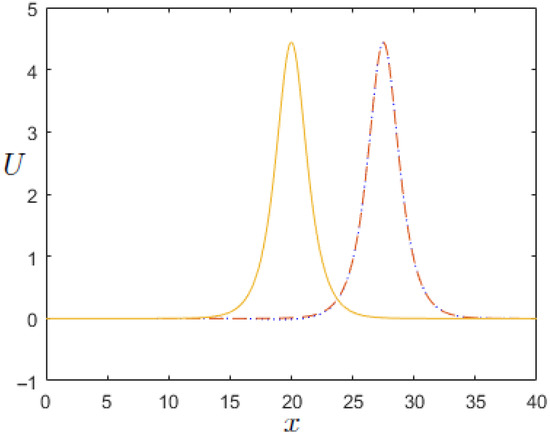
Figure 1. U computed by the numerical scheme $\left(6\right)$–$\left(8\right)$ with $h=0.1$ and $\tau =0.0125$. Comparison between the exact solution and the numerical solution at time $T=5$. Initial condition (solid line); exact solution (dotted line); and numerical solution (dashed line).

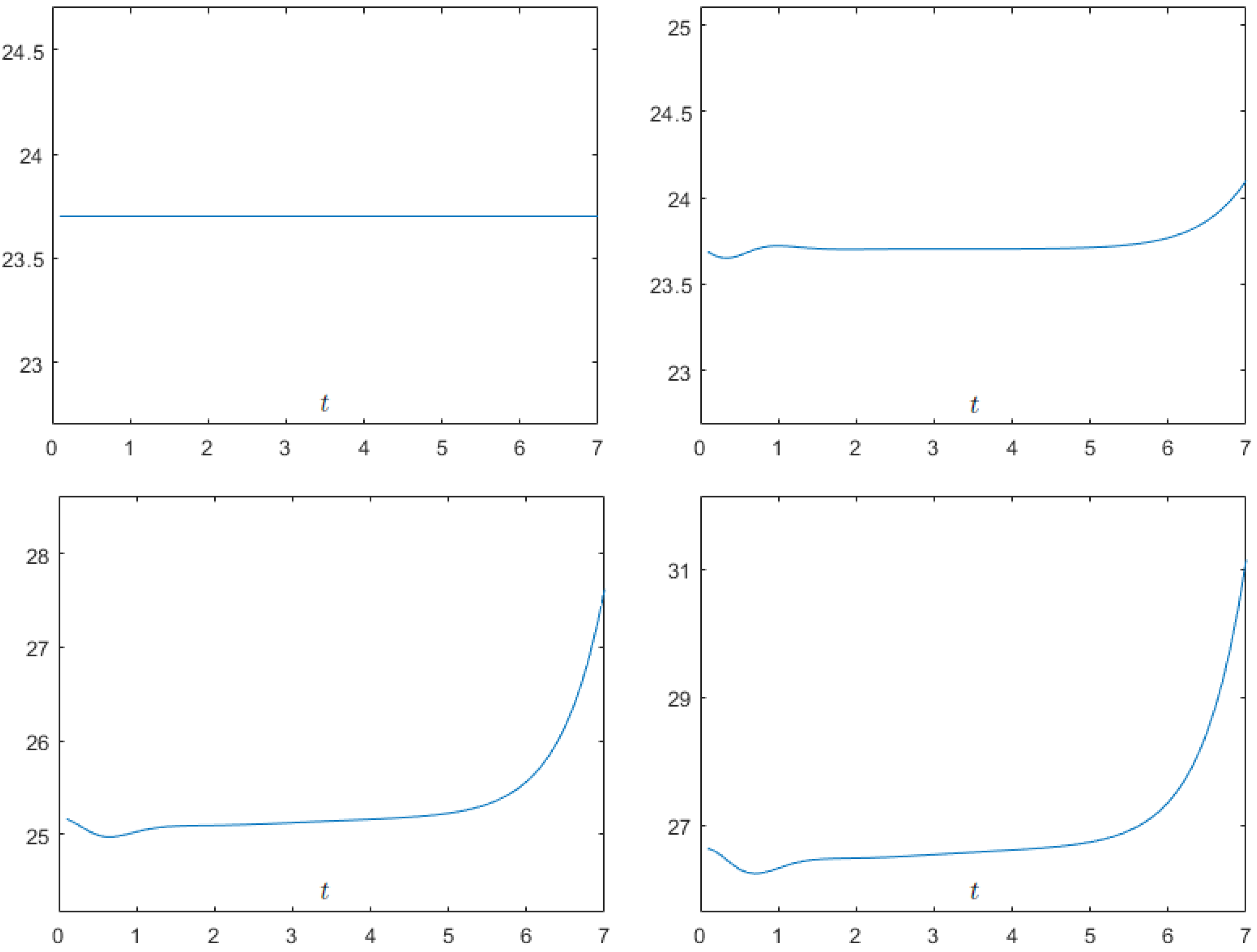
The curves of discrete energy $E^n$ and discrete quantities ${\tilde{E}}^n,$ $Q^n,$ and ${∥U_t^n∥}^2$ obtained by the numerical scheme $\left(6\right)$–$\left(8\right)$ at a larger T value $(T=7)$ are plotted in Figure 2. The figure shows that the numerical scheme $(6$)–$\left(8\right)$ possesses very good conservation properties when compared to the theoretical results.

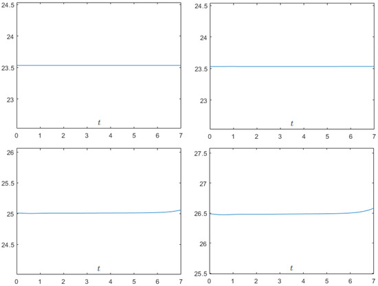
Figure 2. Discrete energy $E^n$ and discrete quantities ${\tilde{E}}^n,$ $Q^n$, and ${∥U_t^n∥}^2$ computed by the numerical scheme $\left(6\right)$–$\left(8\right)$ with $h=0.1$ and $\tau =0.0125$ at time $T=7.$ $E^n$ (Up-Left); ${\tilde{E}}^n$ (Up-Right); $Q^n$ (Down-Left); and ${∥U_t^n∥}^2$ (Down-Right).

In order investigate the influence of the time-step size $\tau$, the computations were repeated with a fixed space step $h=0.1$ and a different time-step size $\tau =0.0125$. Figure 3 shows the sensitivities of $E^n,$ ${\tilde{E}}^n,$ $Q^n,$ and ${∥U_t^n∥}^2$ to the time-step size $\tau$. We can easily see that the discrete quantities ${\tilde{E}}^n,$$Q^n,$ and ${∥U_t^n∥}^2$ are more sensitive than the discrete energy $E^n$ to the changing of the time-step size $\tau .$

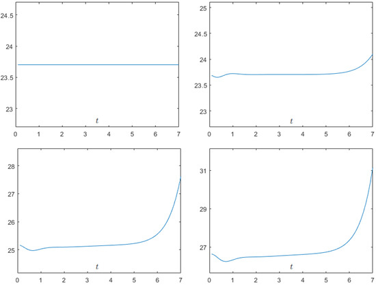
Figure 3. Discrete energy $E^n$ and discrete quantities ${\tilde{E}}^n,$ $Q^n$, and ${∥U_t^n∥}^2$ computed by the numerical scheme $\left(6\right)$–$\left(8\right)$ with $h=\tau =0.1$ at time $T=7.$ $E^n$ (Up-Left); ${\tilde{E}}^n$ (Up-Right); $Q^n$ (Down-Left); and ${∥U_t^n∥}^2$ (Down-Right).

• Kink Solitary Wave Solution

Now, let us consider the following kink solitary wave solution of $\left(31\right)$ given by [33]

$$\begin{array}{cc}\hfill u(x,t)=\sqrt{\frac{\alpha }{\beta }}tanh\left(\sqrt{\frac{\alpha }{2(1-c^2)}}(x-ct)\right),& \left|c\right|<1.\end{array}$$

(33)

This kink solution approaches $\pm \sqrt{\frac{\alpha }{\beta }}$ as $\xi =x-ct\to \pm \infty$. So, for solving $\left(31\right)$, initial conditions can be obtained from this exact solution (Equation $\left(33\right))$ along with the boundary conditions given by

$$\begin{array}{ccc}\hfill u(0,t)=-\sqrt{\frac{\alpha }{\beta }},& u(40,t)=\sqrt{\frac{\alpha }{\beta }},& 0\le t\le T.\hfill \end{array}$$

For computations, we choose $\alpha =1,$ $\beta =\frac{1}{{\pi }^2}$. We solved $\left(31\right)$ with the numerical scheme $\left(6\right)$–$\left(8\right)$ for different velocities c and several values of $\tau$ and $h.$

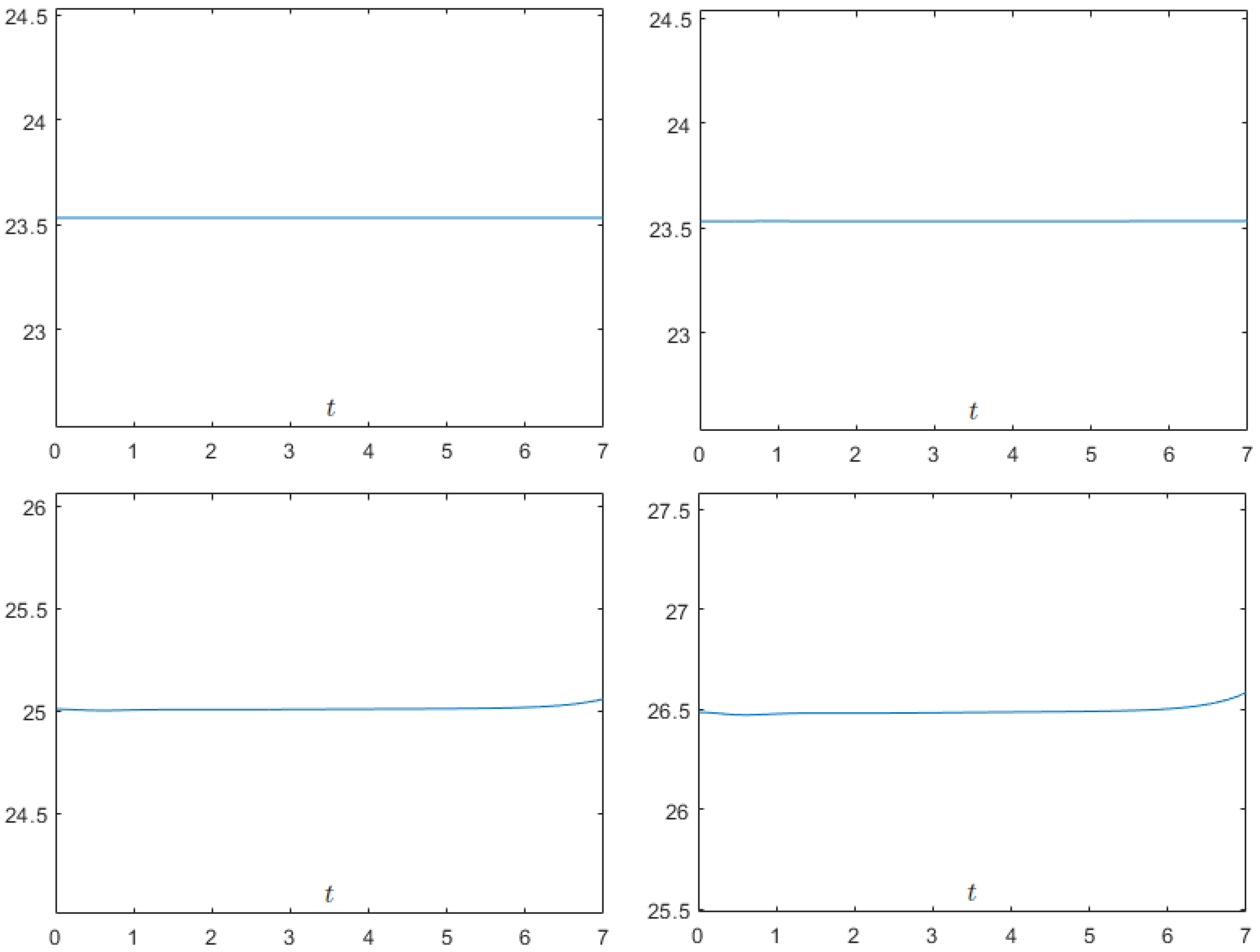
Figure 4 shows the comparison between the exact solution and the numerical solution with $h=0.1$ and $\tau =0.0125$ at time $T=50$ for $c=0.1$. One can easily see that the solitary wave solution computed by the numerical scheme $\left(6\right)$–$\left(8\right)$ agrees very well with the exact solution. In addition, the curves of discrete energy $E^n$ and discrete quantities ${\tilde{E}}^n,$$Q^n$, and ${∥U_t^n∥}^2$ obtained by the numerical scheme $\left(6\right)$–$\left(8\right)$ are plotted in Figure 5. This shows that the numerical scheme $\left(6\right)$–$\left(8\right)$ possesses extremely good conservation properties.

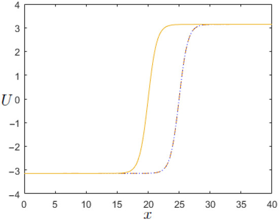
Figure 4. U computed by the numerical scheme $\left(6\right)$–$\left(8\right)$ with $h=0.1$ and $\tau =0.0125$. Comparison between the exact solution and the numerical solution at time $T=50$. Initial condition (solid line); exact solution (dotted line); and numerical solution (dashed line).

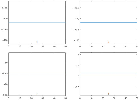
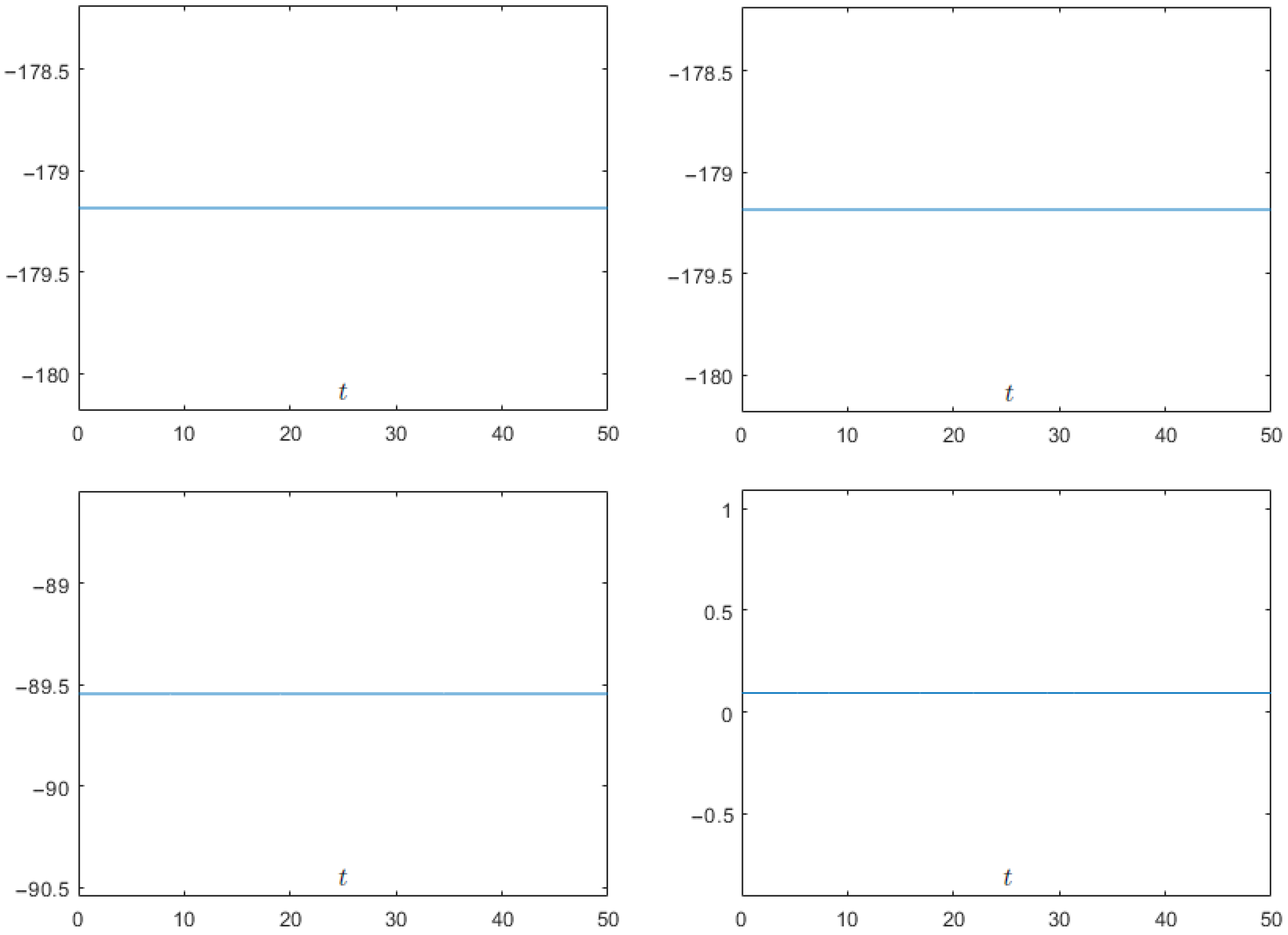
Figure 5. Discrete energy $E^n$ and discrete quantities ${\tilde{E}}^n,$ $Q^n$, and ${∥U_t^n∥}^2$ computed by the numerical scheme $\left(6\right)$–$\left(8\right)$ with $h=0.1$ and $\tau =0.0125$ at time $T=50.$ $E^n$ (Up-Left); ${\tilde{E}}^n$ (Up-Right); $Q^n$ (Down-Left); and ${∥U_t^n∥}^2$ (Down-Right).

Table 1 gives the numerical errors for the scheme $\left(6\right)$–$\left(8\right)$ with different h and $\tau$ at time $T=50$. In fact, the errors are presented for mesh widths h and time steps $\tau$ as they are halved. Using simple arithmetic, one can easily verify that the $L_{\infty }$ error decreases as second order in time and space when $\tau$ and h are halved. Table 2 and Table 3 show the conservation of discrete energy $E^n$ and discrete quantities ${\tilde{E}}^n,$$Q^n,$ and ${∥U_t^n∥}^2$ computed by the numerical scheme $\left(6\right)$–$\left(8\right)$ with $h=\tau =0.1$ at time $T=10,20,30,40,$ and 50. Moreover, Table 4 gives the errors between exact and approximate discrete energies and quantities with different velocities at different times in the case when $h=0.1$ and $\tau =0.0125$.

Table 1. The numerical errors for different h and $\tau$ at time $T=50$.

$\mathit{c}=0.1$	$\mathit{h}=0.1$		$\mathit{h}=0.05$
	${∥e^n∥}_{\infty }$	$∥e^n∥$	${∥e^n∥}_{\infty }$	$∥e^n∥$
$\tau =0.1$	$6.4229947\times {10}^{-3}$	$8.4036315\times {10}^{-3}$	$1.7938245\times {10}^{-3}$	$2.3492447\times {10}^{-3}$
$\tau =0.05$	$6.1916631\times {10}^{-3}$	$8.1103089\times {10}^{-3}$	$1.5889166\times {10}^{-3}$	$2.0859734\times {10}^{-3}$
$\tau =0.025$	$6.1110808\times {10}^{-3}$	$8.0373959\times {10}^{-3}$	$1.5329330\times {10}^{-3}$	$2.0216974\times {10}^{-3}$
$\tau =0.0125$	$6.0895241\times {10}^{-3}$	$8.0190648\times {10}^{-3}$	$1.5191884\times {10}^{-3}$	$2.0056431\times {10}^{-3}$
$\mathit{c}=\mathbf{0.1}$	$\mathit{h}=\mathbf{0.025}$		$\mathit{h}=\mathbf{0.0125}$
	${∥e^n∥}_{\infty }$	$∥e^n∥$	${∥e^n∥}_{\infty }$	$∥e^n∥$
$\tau =0.1$	$6.37524510\times {10}^{-4}$	$8.38629564\times {10}^{-4}$	$3.48616848\times {10}^{-4}$	$4.61523940\times {10}^{-4}$
$\tau =0.05$	$4.42980854\times {10}^{-4}$	$5.82593914\times {10}^{-4}$	$1.56742018\times {10}^{-4}$	$2.06995681\times {10}^{-4}$
$\tau =0.025$	$3.94393863\times {10}^{-4}$	$5.20513898\times {10}^{-4}$	$1.10009011\times {10}^{-4}$	$1.45397726\times {10}^{-4}$
$\tau =0.0125$	$3.82361297\times {10}^{-4}$	$5.05042927\times {10}^{-4}$	$9.84232136\times {10}^{-5}$	$1.30065000\times {10}^{-4}$

Table 2. Discrete energy $E^n$ and discrete quantities ${\tilde{E}}^n,$ $Q^n,$ and ${∥U_t^n∥}^2$ with $h=\tau =c=0.1$.

$\mathit{c}=0.1$	${\mathit{E}}^{\mathit{n}}$	${\tilde{\mathit{E}}}^{\mathit{n}}$	${\mathit{Q}}^{\mathit{n}}$	${∥{\mathit{U}}_{\mathit{t}}^{\mathit{n}}∥}^2$
$T=10$	−179.184654861638	−179.184653840830	−89.54557482415776	0.09350419251447
$T=20$	−179.184654890734	−179.184653061841	−89.54557787387751	0.09349731408601
$T=30$	−179.184654919834	−179.184652734929	−89.54558438427085	0.09348396638753
$T=40$	−179.184654948939	−179.184652618482	−89.54559308985157	0.09346643877978
$T=50$	−179.184654978049	−179.184652779509	−89.54560187973719	0.09344902003472

Table 3. Discrete energy $E^n$ and discrete quantities ${\tilde{E}}^n,$ $Q^n,$ and ${∥U_t^n∥}^2$ with $h=\tau =0.1$ and $c=0.2$.

$\mathit{c}=0.2$	${\mathit{E}}^{\mathit{n}}$	${\tilde{\mathit{E}}}^{\mathit{n}}$	${\mathit{Q}}^{\mathit{n}}$	${∥{\mathit{U}}_{\mathit{t}}^{\mathit{n}}∥}^2$
$T=10$	−178.894785975667	−178.894779071216	−89.25749397503454	0.37979112114713
$T=20$	−178.894786093736	−178.894775141725	−89.25753221833852	0.37971070504812
$T=30$	−178.894786211828	−178.894775717560	−89.25758719130271	0.37960133495474
$T=40$	−178.894786329945	−178.894779939288	−89.25763320390750	0.37951353147354
$T=50$	−178.894786448089	−178.894786332554	−89.25766841880310	0.37944949494802

Table 4. The errors between exact and approximate discrete energies and quantities with different velocities at different times.

$\mathit{Velocity}$	$\mathit{Time}$	$|{\widehat{\mathit{E}}}^{\mathit{n}}-{\mathit{E}}^{\mathit{n}}|$	$|{\widetilde{\widehat{\mathit{E}}}}^{\mathit{n}}-{\tilde{\mathit{E}}}^{\mathit{n}}|$	$|{\widehat{\mathit{Q}}}^{\mathit{n}}-{\mathit{Q}}^{\mathit{n}}|$	${∥{\widehat{\mathit{U}}}_{\mathit{t}}^{\mathit{n}}∥}^2-{∥{\mathit{U}}_{\mathit{t}}^{\mathit{n}}∥}^2$
$c=0.1$	$T=1$	$1.9263239\times {10}^{-8}$	$3.5616346\times {10}^{-7}$	$1.7027686\times {10}^{-5}$	$3.3699209\times {10}^{-5}$
	$T=5$	$1.9263836\times {10}^{-8}$	$2.9341919\times {10}^{-8}$	$6.3929299\times {10}^{-6}$	$1.2815201\times {10}^{-5}$
	$T=10$	$1.9264291\times {10}^{-8}$	$1.2115395\times {10}^{-7}$	$7.3275363\times {10}^{-6}$	$1.4776226\times {10}^{-5}$
$c=0.2$	$T=1$	$3.2929548\times {10}^{-7}$	$1.2054303\times {10}^{-6}$	$7.6424689\times {10}^{-5}$	$1.5164394\times {10}^{-4}$
	$T=5$	$3.2929474\times {10}^{-7}$	$5.2233454\times {10}^{-7}$	$3.1137188\times {10}^{-5}$	$6.2796710\times {10}^{-5}$
	$T=10$	$3.2929548\times {10}^{-7}$	$9.6851493\times {10}^{-7}$	$3.8699464\times {10}^{-5}$	$7.8367444\times {10}^{-5}$
$c=0.3$	$T=1$	$1.8083146\times {10}^{-6}$	$1.8153764\times {10}^{-6}$	$1.9013949\times {10}^{-4}$	$3.7846360\times {10}^{-4}$
	$T=5$	$1.8083150\times {10}^{-6}$	$2.7416199\times {10}^{-6}$	$9.0616743\times {10}^{-5}$	$1.8397510\times {10}^{-4}$
	$T=10$	$1.8083162\times {10}^{-6}$	$3.9544104\times {10}^{-6}$	$1.3546068\times {10}^{-4}$	$2.7487579\times {10}^{-4}$

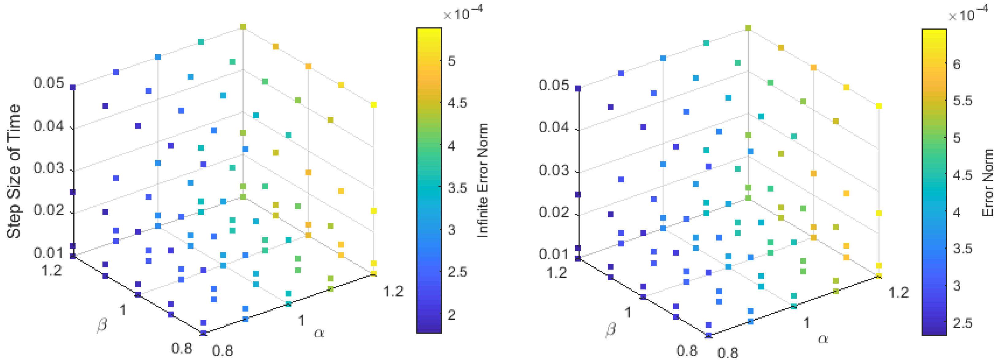
Figure 6 and Figure 7 show the error functions ${∥e^n∥}_{\infty }$ and $∥e^n∥$ with $c=0.2,h=0.1,$ and $\tau =0.05,0.025,0.015,$ and $0.01$ at time $T=1$. The error functions are computed at different values for $\alpha$ and $\beta$. Hence, for a small velocity c, the number of error oscillations decreases as $\alpha$ decreases and $\beta$ increases—i.e., when the cubic term dominates the linear term in the Klein–Gordon nonlinearity.

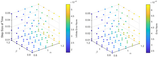
Figure 6. The error functions ${∥e^n∥}_{\infty }$ and $∥e^n∥$ computed when $\alpha$ equals $0.8,0.9,1.0,1.1,$ and $1.2$ and $\beta$ equals $0.8,0.9,1.0,1.1,$ and $1.2$.

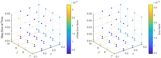
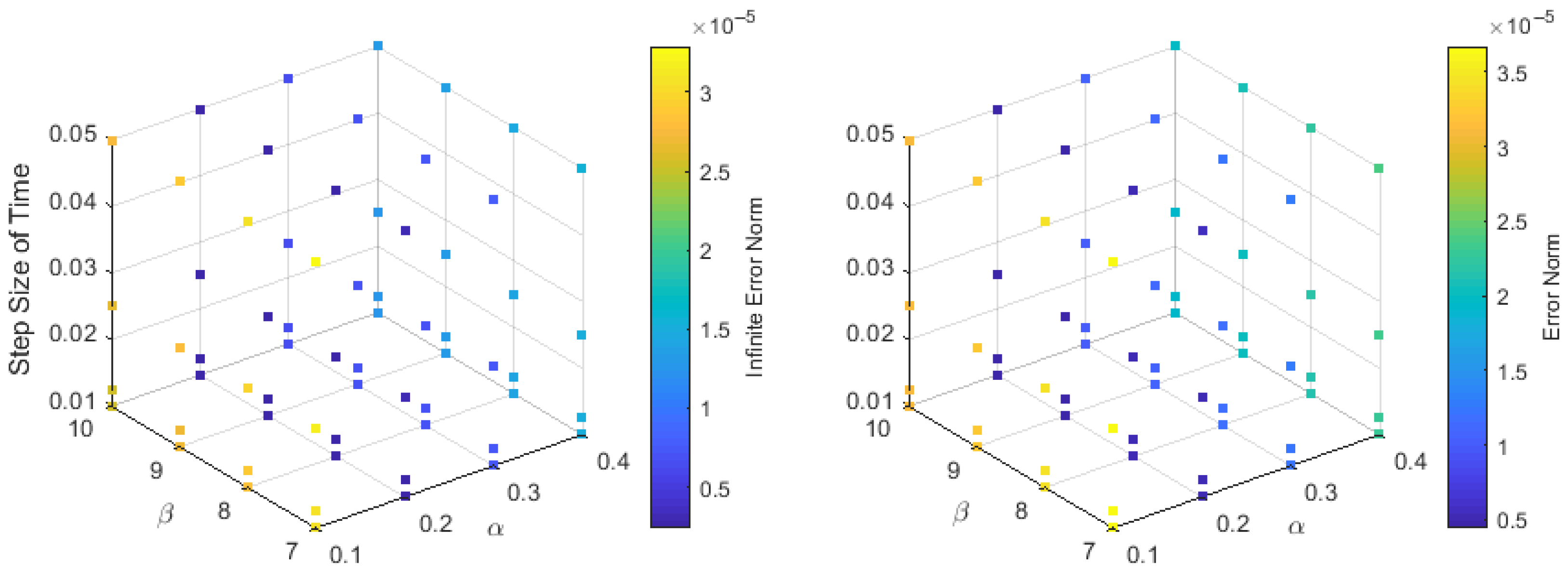
Figure 7. The error functions ${∥e^n∥}_{\infty }$ and $∥e^n∥$ computed when $\alpha$ equals $0.1,0.2,0.3,$ and $0.4$ and $\beta$ equals $7,8,9,$ and 10.

6. Conclusions

In this paper, we constructed a finite difference scheme that conserves the discrete energy (and some other discrete quantities) for solving the Klein–Gordon equation with cubic nonlinearity. Theoretical analysis is provided to show the conservation properties of the numerical scheme. In addition, we obtain theoretical error estimates and prove the stability and the convergence of the scheme. Finally, we carry out a number of computer simulations using the scheme. In particular, we consider the cases where the solutions are either traveling pulses or traveling wave fronts. The numerical simulations demonstrate that our method performs very well in both instances—conserving the discrete energies and producing accurate and stable solutions. One observation is that if it is imperative to conserve the other discrete quantities along with the discrete energy, one may have to choose a smaller time step. This is because since the conservation of the discrete quantities are correct up to the order of the spatial mesh and the time step, at instances, some of the discrete quantities, other than the discrete energy, are susceptible to an increasing time step. However, this does not affect the performance of our method. One can still conserve the discrete energy and obtain excellent numerical results that are stable and accurate. In addition, in the case of traveling wave fronts with low speeds, we find that our scheme performs well (with no error oscillations) if the cubic term is dominant compared to the linear term (i.e., larger $\beta$ and smaller $\alpha$). As we noted in the introduction, there are a few energy conserving explicit finite difference schemes in the literature for solving the Klein–Gordon equation. However, because of the explicitness, the stability of these schemes is conditional resulting in restrictive choices for the spatial mesh width and time step. In contrast, since our energy-conserving scheme is an implicit scheme, the stability is unconditional, and we do not have any restrictions on the spatial mesh width or the time step. As pointed out in [29], an energy-conserving scheme is very suitable for studying the long-time behavior of wave solutions. For example, the wave collisions and resonance behavior that were studied decades ago in [4] could be well understood if one employs an implicit method such as ours that does not dissipate energy. At this juncture, one should note that another interesting equation with cubic nonlinearity is the nonlinear Schrödinger equation [34]. An energy-conserving circularly exact leapfrog scheme was developed in [34] to study the nonlinear Schrödinger equation. However, our work could be easily modified to study the nonlinear Schrödinger equation as well. Further, this work could be extended to Klein–Gordon equations with other nonlinearities. For instance, if the nonlinear term in Equation $\left(2\right)$ is $\beta u^q$, where $q=2^p-1$ and p is any positive integer (note that, $p=2$ gives $u^3$), one could construct a numerical scheme such that in Equation $\left(6\right)$, the nonlinear term is split judiciously as

$$\begin{array}{c}\mathrm{for}p=2\hfill \\ \frac{\beta }{2^2}\left({U_m}^{n+1}+{U_m}^{n-1}\right)\left({\left({U_m}^{n+1}\right)}^2+{\left({U_m}^{n-1}\right)}^2\right),\hfill \\ \mathrm{for}p=3\hfill \\ \frac{\beta }{2^3}\left({U_m}^{n+1}+{U_m}^{n-1}\right)\left({\left({U_m}^{n+1}\right)}^2+{\left({U_m}^{n-1}\right)}^2\right)\left({\left({U_m}^{n+1}\right)}^4+{\left({U_m}^{n-1}\right)}^4\right),\hfill \\ \mathrm{for}p=4\hfill \\ \frac{\beta }{2^4}\left({U_m}^{n+1}+{U_m}^{n-1}\right)\left({\left({U_m}^{n+1}\right)}^2+{\left({U_m}^{n-1}\right)}^2\right)\left({\left({U_m}^{n+1}\right)}^4+{\left({U_m}^{n-1}\right)}^4\right)\left({\left({U_m}^{n+1}\right)}^8+{\left({U_m}^{n-1}\right)}^8\right),\hfill \end{array}$$

and more generally as,

$$\begin{array}{c}\frac{\beta }{2^p}\left({U_m}^{n+1}+{U_m}^{n-1}\right)\left({\left({U_m}^{n+1}\right)}^2+{\left({U_m}^{n-1}\right)}^2\right)\left({\left({U_m}^{n+1}\right)}^4+{\left({U_m}^{n-1}\right)}^4\right)\cdots \left({\left({U_m}^{n+1}\right)}^r+{\left({U_m}^{n-1}\right)}^r\right),\hfill \end{array}$$

where $r=2^{(p-1)}$. Then, as in Section 2, one could proceed to show that the scheme will be energy conserving for any positive integer p. So, the idea of re-arranging the nonlinearity in a judicious manner could even be adopted in combination with the standard discretization of fractional derivatives in order to develop new and efficient numerical schemes for the fractional nonlinear Klein–Gordon equations. Therefore, we believe that our work adds to the body of knowledge with regards to the computational study of Klein–Gordon equations.

References

- Caudrey, P.J.; Eilbeck, J.C.; Gibbon, J.D. The sine-Gordon equation as a model classical field theory. Il Nuovo Cimento B 1975, 25, 497–512. [Google Scholar] [CrossRef]
- Dodd, R.K.; Morris, H.C.; Eilbeck, J.C.; Gibbon, J.D. Soliton and Nonlinear Wave Equations; Academic Press: London, UK; New York, NY, USA, 1982. [Google Scholar]
- Wazwaz, A.M. New travelling wave solutions to the Boussinesq and the Klein–Gordon equations. Commun. Nonlinear Sci. Numer. Simul. 2008, 13, 889–901. [Google Scholar] [CrossRef]
- Manoranjan, V.S. Some numerical experiments on Higgs model. Comput. Phys. Commun. 1983, 29, 1–5. [Google Scholar] [CrossRef]
- Alzaleq, L.M.; Manoranjan, V. Qualitative analysis and exact traveling wave solutions for the Klein-Gordon equation with quintic nonlinearity. Phys. Scr. 2019, 94, 085208. [Google Scholar] [CrossRef]
- Amin, M.; Abbas, M.; Iqbal, M.K.; Baleanu, D. Numerical Treatment of Time-Fractional Klein–Gordon Equation Using Redefined Extended Cubic B-Spline Functions. Front. Phys. 2020, 8, 288. [Google Scholar] [CrossRef]
- Golmankhaneh, A.K.; Golmankhaneh, A.K.; Baleanu, D. On nonlinear fractional Klein–Gordon equation. Signal Process. 2011, 91, 446–451. [Google Scholar] [CrossRef]
- Kurulay, M. Solving the fractional nonlinear Klein-Gordon equation by means of the homotopy analysis method. Adv. Differ. Equations 2012, 2012, 187. Available online: http://www.advancesindifferenceequations.com/content/2012/1/187 (accessed on 2 November 2012). [CrossRef] [Green Version]
- Li, C.; Zeng, F. Finite Difference Methods for Fractional Differential Equations. Int. J. Bifurc. Chaos 2012, 22, 1230014. [Google Scholar] [CrossRef]
- Liu, J.; Nadeem, M.; Habib, M.; Akgül, A. Approximate Solution of Nonlinear Time-Fractional Klein-Gordon Equations Using Yang Transform. Symmetry 2022, 14, 907. [Google Scholar] [CrossRef]
- Nagy, A.M. Numerical solution of time fractional nonlinear Klein-Gordon equation using Sinc-Chebyshev collocation method. Appl. Math. Comput. 2017, 310, 139–148. [Google Scholar] [CrossRef]
- Strauss, W.; Vazquez, L. Numerical solution of a nonlinear Klein-Gordon equation. J. Comput. Phys. 1978, 28, 271–278. [Google Scholar] [CrossRef]
- Li, S.; Vu-Quoc, L. Finite difference calculus invariant structure of a class of algorithms for the nonlinear Klein-Gordon equation. SIAM J. Numer. Anal. 1995, 32, 1839–1875. [Google Scholar] [CrossRef]
- Abbasbandy, S. Numerical solution of non-linear Klein-Gordon equations by variational iteration method. Int. J. Numer. Methods Eng. 2007, 70, 876–881. [Google Scholar] [CrossRef]
- Shakeri, F.; Dehghan, M. Numerical solution of the Klein-Gordon equation via He’s variational iteration method. Nonlinear Dyn. 2008, 51, 89–97. [Google Scholar] [CrossRef]
- Aslanov, A. The homotopy-perturbation method for solving klein-gordon-type equations with unbounded right-hand side. Z. Naturforschung A 2009, 64, 149–152. [Google Scholar] [CrossRef]
- Yousif, M.A.; Mahmood, B.A. Approximate solutions for solving the Klein–Gordon and sine-Gordon equations. J. Assoc. Arab. Univ. Basic Appl. Sci. 2017, 22, 83–90. [Google Scholar] [CrossRef] [Green Version]
- Dehghan, M.; Shokri, A. Numerical solution of the nonlinear Klein-Gordon equation using radial basis functions. J. Comput. Appl. Math. 2009, 230, 400–410. [Google Scholar] [CrossRef] [Green Version]
- Khuri, S.A.; Sayfy, A. A spline collocation approach for the numerical solution of a generalized nonlinear Klein-Gordon equation. Appl. Math. Comput. 2010, 216, 1047–1056. [Google Scholar] [CrossRef]
- Mohebbi, A.; Asgari, Z.; Shahrezaee, A. Fast and high accuracy numerical methods for the solution of nonlinear Klein-Gordon equations. Z. Naturforschung A 2011, 66, 735–744. [Google Scholar] [CrossRef]
- Dutykh, D.; Chhay, M.; Clamond, D. Numerical study of the generalised Klein–Gordon equations. Phys. D Nonlinear Phenom. 2015, 304, 23–33. [Google Scholar] [CrossRef] [Green Version]
- Shukla, H.S.; Tamsir, M. Numerical solution of nonlinear sine–Gordon equation by using the modified cubic B-spline differential quadrature method. Beni-Suef Univ. J. Basic Appl. Sci. 2018, 7, 359–366. [Google Scholar] [CrossRef]
- El-Sayed, S.M. The decomposition method for studying the Klein–Gordon equation. Chaos Solitons Fractals 2003, 18, 1025–1030. [Google Scholar] [CrossRef]
- Zhang, J.; Kong, L. New energy-preserving schemes for Klein-Gordon-Schrödinger equations. Appl. Math. Model. 2016, 40, 6969–6982. [Google Scholar] [CrossRef]
- He, Y. High-Order Energy and Linear Momentum Conserving Methods for the Klein-Gordon Equation. Mathematics 2018, 6, 200. [Google Scholar] [CrossRef] [Green Version]
- Wang, B.; Wu, X. The formulation and analysis of energy-preserving schemes for solving high-dimensional nonlinear Klein-Gordon equations. IMA J. Numer. Anal. 2019, 39, 2016–2044. [Google Scholar] [CrossRef]
- Kumbinarasaiah, S.; Ramane, H.S.; Pise, K.S.; Hariharan, G. Numerical-solution-for-nonlinear-klein–gordon equation via operational-matrix by clique polynomial of complete graphs. Int. J. Appl. Comput. Math. 2021, 7, 1–19. [Google Scholar] [CrossRef]
- Kanth, A.R.; Aruna, K. Differential transform method for solving the linear and nonlinear Klein–Gordon equation. Comput. Phys. Commun. 2009, 180, 708–711. [Google Scholar] [CrossRef]
- Jiménez, S.; Vázquez, L. Analysis of four numerical schemes for a nonlinear Klein-Gordon equation. Appl. Math. Comput. 1990, 35, 61–94. [Google Scholar] [CrossRef]
- Wang, T.; Chen, J.; Zhang, L. Conservative difference methods for the Klein-Gordon-Zakharov equations. J. Comput. Appl. Math. 2007, 205, 430–452. [Google Scholar] [CrossRef]
- Chen, J.; Zhang, L. Two energy conserving numerical schemes for the Klein-Gordon-Zakharov equations. J. Appl. Math. 2013, 2013, 46208. [Google Scholar] [CrossRef] [Green Version]
- Zhou, Y. Applications of Discrete Functional Analysis to the Finite Difference Method; Pergamon Press: Oxford, UK, 1991. [Google Scholar]
- Alzaleq, L.M. A Klein-Gordon Equation Revisited: New Solutions and a Computational Method. Ph.D. Thesis, Washington State University, Pullman, WA, USA, 2016. [Google Scholar]
- Sanz-Serna, J.M.; Manoranjan, V.S. A Method for the Integration in Time of Certain Partial Differential Equations. J. Comput. Phys. 1983, 52, 273–289. [Google Scholar] [CrossRef]
Publisher’s Note: MDPI stays neutral with regard to jurisdictional claims in published maps and institutional affiliations. |
© 2022 by the authors. Licensee MDPI, Basel, Switzerland. This article is an open access article distributed under the terms and conditions of the Creative Commons Attribution (CC BY) license (https://creativecommons.org/licenses/by/4.0/).