Long-Term Side Effects: A Mathematical Modeling of COVID-19 and Stroke with Real Data

Abstract

The post-effects of COVID-19 have begun to emerge in the long term in society. Stroke has become one of the most common side effects in the post-COVID community. In this study, to examine the relationship between COVID-19 and stroke, a fractional-order mathematical model has been constructed by considering the fear effect of being infected. The model’s positivity and boundedness have been proved, and stability has been examined for disease-free and co-existing equilibrium points to demonstrate the biological meaningfulness of the model. Subsequently, the basic reproduction number (the virus transmission potential (${\mathcal{R}}_0$)) has been calculated. Next, the sensitivity analysis of the parameters according to ${\mathcal{R}}_0$ has been considered. Moreover, the values of the model parameters have been calculated using the parameter estimation method with real data originating from the United Kingdom. Furthermore, to underscore the benefits of fractional-order differential equations (FODEs), analyses demonstrating their relevance in memory trace and hereditary characteristics have been provided. Finally, numerical simulations have been highlighted to validate our theoretical findings and explore the system’s dynamic behavior. From the findings, we have seen that if the screening rate in the population is increased, more cases can be detected, and stroke development can be prevented. We also have concluded that if the fear in the population is removed, the infection will spread further, and the number of people suffering from a stroke may increase.

1. Introduction

Coronaviruses encompass a group of viruses capable of inducing ailments such as the common cold, severe acute respiratory syndrome (SARS), and Middle East respiratory syndrome (MERS). In 2019, a new type of coronavirus caused the pandemic. The virus has been identified as severe acute respiratory syndrome coronavirus 2 (SARS-CoV-2). The consequent illness is called novel coronavirus disease 2019 (COVID-19). In March 2020, the World Health Organization proclaimed coronavirus (COVID-19) as a worldwide pandemic. More than two and a half years after the spread of the epidemic, and despite the decline in infections in various parts of the world, many are still infected. Vaccines have helped achieve this triumph of regression since the doses allow the body’s defenses to safely “train” to fight off the pathogen even before exposure.

Unfortunately, in some cases, the virus can reach vital organs (such as the lungs), leading to severe inflammatory conditions. These situations usually require emergency care and represent a significant risk because they may be fatal. Although long-term COVID is still shrouded in much mystery, the US Centers for Disease Control and Prevention (CDC) estimates that up to 13.3 percent of people with coronavirus experience long-term symptoms for a month or more. Moreover, about 2.5 percent reported symptoms lasting at least three months. Recently, many studies have focused on the side effects of infection with COVID-19 [1,2,3]. Perhaps the most important of these side effects is the increased incidence of chronic diseases, even among young people. These diseases may be due to genetic factors or an unhealthy lifestyle, and a new study has revealed the relationship between infection and an increased risk of developing neurodegenerative disorders. The study was presented at the eighth conference of the European Academy of Neurology and included the analysis of the health records of more than half of the population of Denmark, between February 2020 and November 2021. The researchers analyzed the statistics of inpatient and outpatient clinics in Denmark. A total of 919,731 people were studied, including 43,375 who had been confirmed to have previously been infected with the coronavirus, and the results showed that their risk of stroke was 2.7 times higher than that of others. In September 2020, this was first noticed by a team of scientists led by Mark Ellul, PhD, NIHR Clinical Lecturer in Neurology at the Institute of Infection, Veterinary and Ecological Sciences from the University of Liverpool. They discovered that the total number of hospitalized patients with a large vessel stroke who also had a COVID-19 diagnosis was seven times higher than usual (https://www.ean.org/congress2022 (accessed on 7 September 2023)).

Over the past months, doctors have noticed several data indicating a link between COVID-19 and stroke. Strokes occur when the blood supply to the brain is interrupted, such as when a blood clot or blockage occurs. This leads to an ischemic stroke, or when an artery in the brain ruptures and bleeding occurs, a hemorrhagic stroke. Ischemic strokes are the most common. The effects of corona are not limited to the lung; there are changes in the work of organs and cells in several places in the body, and the virus also stimulates the response of our immune system, which naturally produces chemicals in our bodies, which causes more changes in the way cells work. These biological changes can increase the risk of a blood clot forming, increasing stroke risk. One possible explanation is that severe cases of COVID-19 can lead to multi-organ failure, including kidney failure. Serious illness and multi-organ failure can increase the risk of stroke. It is also believed that COVID-19 affects the blood clotting system in the body, and appears to promote clot formation [4,5]. The coronavirus may cause a stroke about nine days after the onset of symptoms in a person, and experts say that a stroke can occur in any patient with COVID-19, regardless of age, and even those who have few or no symptoms; many people with COVID-19 under the age of 30 have suffered strokes even when their symptoms were mild [6].

It has been proven that the coronavirus may cause the development of tiny clots or “small clots” (microthrombi), and these clots can move to the lung and impede blood flow to it, which is a “pulmonary embolism”, or move to the blood circulation of the brain and cause a stroke [7,8].

Studies are essential for controlling epidemics because they may be used to predict how an epidemic will evolve in the future, pinpoint the critical tactics for stopping its spread, and issue the necessary alerts before it spirals out of control and kills many people. Numerous scholarly papers spanning various disciplines delve into predicting, exploring, and advancing crucial approaches to addressing COVID-19 and chronic conditions. Historically, various mathematical models have been employed to simulate diverse epidemics. Indeed, these models have demonstrated their efficacy and value as tools for disease identification, prediction, and treatment. Numerous illnesses are mathematically modeled today to determine the most effective treatment strategies [9,10,11].

The insights derived from fractional-order equations continue to excel in representing real phenomena compared to integer-order equations, even though using integer-order equations achieves a certain level of success. Specific attributes distinctive to this equation format, such as recurrent operations and nonlocal characteristics, which ensure that the current state of the mathematical model is compatible with earlier and later states, are among the benefits of mathematical modeling using FDEs. FDEs can be used to replicate this event correctly. They also have genetic characteristics and are inherently connected to memory systems seen in many epidemic disorders. Additionally, FDEs assist us in minimizing potential mistakes that can result from modeling parameters that cannot be considered. In addition to being more accurate when discussing biological and medical phenomena, the memory impact of dynamic behavior and nonlocal features is also tied to earlier historical factors, making the models that rely on these equations more realistic. FODEs have recently emerged as a trustworthy and systematic mathematical instrument for investigating several scientific and engineering phenomena. A wide array of fields, spanning control systems, fluid mechanics, bioengineering, management, financial systems, traffic flow, pollution control, and beyond, have benefited from research in fractional-order differential equations [12,13,14,15,16,17,18,19].

Özköse et al. [20] presented a novel approach to utilizing a fractional-order model, investigating the Congo’s COVID-19 and cholera outbreaks. Naik et al. [21] investigate the critical normal form coefficients for the one-parameter and two-parameter bifurcations of a discrete-time Bazykin–Berezovskaya prey–predator model. In [22], the authors provided a model for the novel coronavirus illness that employs the fractional-order Caputo derivative, different hospitalization plans for severe and moderate cases, and an awareness campaign. In another study [23], the paper focused on fractional derivative mathematical modeling and analysis of the diabetes mellitus model without hereditary components. In [24], Alkahtani et al. analyzed the mathematical COVID-19 model using a fractional-order Caputo operator while considering an asymptomatic class. In [25], a fractional-order coronavirus disease model was built with five compartments. The study examined the effects of successive optimal control strategies in various susceptible classes. In [26], the fractional-order model with vaccination efficacy and declining immunity was examined. Dababneh et al., in [27], presented a new fractional discrete-time COVID-19 model that has the number of people who have received vaccinations as a new state variable in the system equations.

To give examples of some articles that examine the relationship between COVID-19 and stroke biologically, Khedr et al. [28] compared the efficacy and safety of tissue plasminogen activator (rTPA) in acute ischemic stroke (AIS) patients with or without COVID-19 infection. Massoud et al. [29] showed that the risk of stroke appears significant in the first week following infection with COVID-19 but drops to insignificance two weeks later. Zuin et al. [30] compared the risk of incident ischemic stroke among adult COVID-19-infected patients who had recovered to the level of uninfected patients (controls), defined as those who had not contracted the infection over the same follow-up period. Van et al. [31] conducted a systematic evaluation to identify the impact of the COVID-19 pandemic on the presentation and care of stroke in individuals over 65 worldwide. In addition, in ref. [32], Ferrone et al. following the preferred reporting items for systematic review and meta-analyses (PRISMA) recommendations, conducted a systematic review and meta-analysis.

As far as we know from our literature research, there is no fractional-order mathematical model examining the relationship between COVID-19 and stroke, one of the most critical and fatal post-effects of COVID-19, found in the literature. Based on this gap in the literature and motivated by the above studies, in this paper, we have discussed stroke with the fear of getting COVID-19 (which occurs due to dirty information, propaganda, and the effects of social media during the spread of infection in society). We can draw parallels to an experimental study that revealed a remarkable insight by likening the virus to a predator and civilians to prey. Beyond the direct lethality, the very fear instilled by the virus (akin to predation fears) can curtail the growth rate of the prey (akin to a psychological effect), resulting in a notable reduction of 40 percent [33]. Indeed, this analogy brings an intriguing facet of our present situation to the forefront.

The paper is organized into sections: Section 2 introduces the fundamental definitions of fractional calculus (FC). In Section 3, the fractional model has been introduced. In Section 4, the existence and uniqueness of the model’s solution are demonstrated. In the corresponding Section (Section 5), the paper addresses the positivity and boundedness of the solution, along with the stability analysis of the proposed model’s equilibrium points. The basic reproduction number ($R_0$) calculation is also included. In Section 6, sensitivity analysis has been conducted to explore the parameter impacts on the primary reproduction number $R_0$. Section 7 focuses on the examination of the parameter estimation method. In Section 8, the system’s memory effect is explicitly demonstrated. In Section 9, the Adams–Bashforth–Moulton method is employed to compute numerical solutions for our proposed model. Last, a summary of the present study is provided in Section 10.

2. Preliminaries

The subsequent definitions outline the key concepts of FC utilized in this investigation.

Definition 1 

([34]). The fractional integral of the function $\rho \left(t\right)$, $t>0$, of order $\vartheta >0$, is provided by

$$I^{\vartheta }\rho \left(t\right)={\int }_0^t\frac{{(t-s)}^{\vartheta -1}}{\mathsf{\Gamma }\left(\vartheta \right)}\rho \left(s\right)ds.$$

and the fractional derivative (FD) of $\rho \left(t\right),t>0$ of order $\vartheta$ in $(n-1,n)$ is determined by

$$D^{\vartheta }\rho \left(t\right)=I^{n-\vartheta }{D}^n\rho \left(t\right)(D=\frac{d}{dt}),where\mathsf{\Gamma }(.)isGammafunction,\vartheta >0.$$

Definition 2 

([34]). The Laplace transform (LT) of the Caputo derivative of order $\vartheta >0$ for a given function $\rho \left(t\right)$ is defined as follows:

$$L\left[{{}_0^{C}D}_t^{\vartheta }\rho \left(t\right)\right]=s^{\vartheta }\rho \left(s\right)-\sum _{v=0}^{n-1}{\rho }^v\left(0\right)s^{\vartheta -v-1}.$$

(1)

Definition 3 

([34]). The Laplace transform (LT) of the function $\rho \left(t\right)=t^{{\vartheta }_1-1}{E}_{\vartheta ,{\vartheta }_1}(\pm ϵt^{\vartheta })$ is defined as

$$L\left[t^{{\vartheta }_1-1}{E}_{\vartheta ,{\vartheta }_1}(\pm ϵt^{\vartheta })\right]=\frac{s^{\vartheta -{\vartheta }_1}}{s^{\vartheta }\pm ϵ},$$

(2)

where $E_{\vartheta ,{\vartheta }_1}$ is a Mittag-Leffler function.

Theorem 1 

([35,36]). Consider the fractional-order system shown below:

$$\frac{d^{\vartheta }x}{d{t}^{\vartheta }}=f\left(x\right),x\left(0\right)=x_0,$$

(3)

with $\vartheta \in$ (0,1] and $x\in R^n$. The function’s zeros $f\left(X^{*}\right)=0$ are the system’s equilibrium points, and these equilibrium points are:

(1) 

Asymptomatically stable ⇔ the eigenvalues ${\lambda }_i,$ of the Jacobian matrix $J\left(X^{*}\right)$ satisfy that $|arg\left({\lambda }_i\right)|>\frac{\vartheta \pi }{2}.$$\forall i$, $i=1,2,\dots ,n.$

(2) 

Stable ⇔ is asymptomatically stable or the eigenvalues ${\lambda }_i,$$i=1,2,\dots ,n$ of $J\left(X^{*}\right)$ that satisfy $|arg\left({\lambda }_i\right)|=\frac{\vartheta \pi }{2}$ if have the same geometric and algebraic multiplicity.

(3) 

Unstable ⇔$\exists i,$ such that the corresponding eigenvalue ${\lambda }_i$ of $J\left(X^{*}\right)$ satisfy $|arg\left({\lambda }_i\right)|<\frac{\vartheta \pi }{2},$$i=1,2,\dots ,n.$

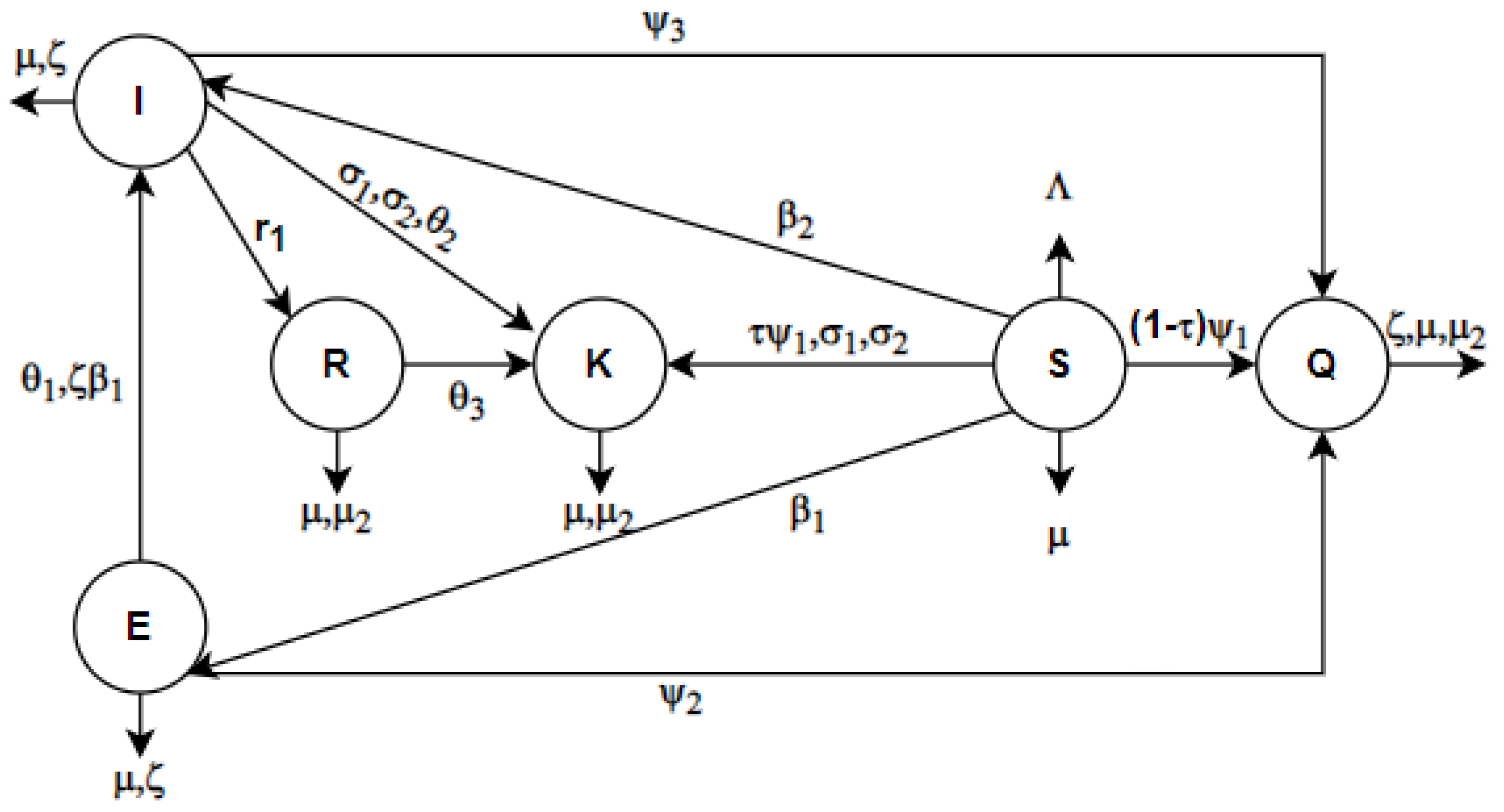
3. Mathematical Modeling

Mathematical models play a crucial role in representing infectious diseases, enabling us to forecast the scope and intensity of such illnesses. Mathematical models offer a means to formulate strategies for treating numerous diseases and mitigating their dissemination. The COVID-19 pandemic, which has persisted for over two years up to the present, has been depicted through various mathematical models. These models also elucidate the extent of COVID-19’s side influence on various other diseases. Some of these models incorporated the vaccination factor, while others factored in the quarantine measures implemented to curtail the disease’s transmission. Some models have presented mathematical models focusing on chronic conditions such as diabetes to also show the impact of COVID-19 on diverse types of diseases [9]. This study has introduced a model dedicated to investigating stroke, a critical repercussion of COVID-19 affecting patients. We have categorized the population into six distinct sub-groups, encompassing susceptible individuals, those in an exposed state, COVID-19-infected cases, individuals who have recovered, those under quarantine, and individuals who have experienced a stroke. We have also included the fear effect in the vulnerable susceptible class to make our model even more comprehensive. In our notation, a healthy and susceptible individual is represented by “S”, an individual in the latent period and not yet infected is denoted as “E”, an individual infected with COVID-19 is indicated as “I”, the recovered population is denoted as “R”, and those in isolation are designated as “Q”. Individuals who have suffered a stroke are represented by “K”. Thus, the total population is also described as $N\left(t\right)=S\left(t\right)+E\left(t\right)+I\left(t\right)+R\left(t\right)+Q\left(t\right)+K\left(t\right).$ One fear function in our model $\frac{1}{1+k_1^{\vartheta }I}.$ $k_1$ indicates the level of fear of getting infected with the virus. Our model has been constructed as below:

$$\begin{array}{ccc}\hfill {{}_0^{C}D}_t^{\vartheta }S& =& {\mathsf{\Lambda }}^{\vartheta }-({\mu }^{\vartheta }+\frac{{\beta }_1^{\vartheta }E}{N}+\frac{{\beta }_2^{\vartheta }I}{N}+{\psi }_1^{\vartheta }+{\sigma }_1^{\vartheta }+{\sigma }_2^{\vartheta })S+{\omega }^{\vartheta }S(1-\frac{S}{C^{\vartheta }})(\frac{1}{1+k_1^{\vartheta }I}),\hfill \\ \hfill {{}_0^{C}D}_t^{\vartheta }E& =& {\beta }_1^{\vartheta }(1-{\eta }^{\vartheta })\frac{ES}{N}-({\mu }^{\vartheta }+{\psi }_2^{\vartheta }+{\theta }_1^{\vartheta }+{\zeta }^{\vartheta })E,\hfill \\ \hfill {{}_0^{C}D}_t^{\vartheta }I& =& {\beta }_1^{\vartheta }{\eta }^{\vartheta }\frac{SE}{N}+{\beta }_2^{\vartheta }\frac{SI}{N}+{\theta }_1^{\vartheta }E-({\mu }^{\vartheta }+r_1^{\vartheta }+{\psi }_3^{\vartheta }+{\sigma }_1^{\vartheta }+{\sigma }_2^{\vartheta }+{\zeta }^{\vartheta }+{\theta }_2^{\vartheta })I,\hfill \\ \hfill {{}_0^{C}D}_t^{\vartheta }R& =& r_1^{\vartheta }I-({\mu }^{\vartheta }+{\mu }_2^{\vartheta }+{\theta }_3^{\vartheta })R,\hfill \\ \hfill {{}_0^{C}D}_t^{\vartheta }Q& =& (1-{\tau }^{\vartheta }){\psi }_1^{\vartheta }S+{\psi }_2^{\vartheta }E+{\psi }_3^{\vartheta }I-({\mu }^{\vartheta }+{\mu }_2^{\vartheta }+{\zeta }^{\vartheta })Q,\hfill \\ \hfill {{}_0^{C}D}_t^{\vartheta }K& =& ({\sigma }_1^{\vartheta }+{\sigma }_2^{\vartheta })(S+I)+{\tau }^{\vartheta }{\psi }_1^{\vartheta }S+{\theta }_2^{\vartheta }I+{\theta }_3^{\vartheta }R-({\mu }^{\vartheta }+{\mu }_2^{\vartheta })K,\hfill \end{array}$$

(4)

with initial conditions:

$$\begin{array}{cc}\hfill & S\left(0\right)=S_0\ge 0,E\left(0\right)=E_0\ge 0,I\left(0\right)=I_0\ge 0,R\left(0\right)=R_0\ge 0,Q\left(0\right)=Q_0\ge 0,K\left(0\right)=K_0\ge 0.\end{array}$$

Figure 1 shows the state variables in model (4) and transitions between them.

Table 1. Parameter values and biological descriptions.

Parameters	Parameter Description
${\mathsf{\Lambda }}^{\vartheta }$	Recruitment rate
${\mu }^{\vartheta }$	Natural death probability
${\mu }_2^{\vartheta }$	Death rate from stroke
${\beta }_1^{\vartheta }$	Transmission rate for E class
${\beta }_2^{\vartheta }$	Transmission rate for I class
${\omega }^{\vartheta }$	Growth rate
$k_1^{\vartheta }$	Level of the fear to be infected with COVID-19
$C^{\vartheta }$	Carrying capacity of S
${\psi }_1^{\vartheta }$	Rate of susceptible individuals undergoing quarantine
${\psi }_2^{\vartheta }$	Rate of infected individuals without symptoms who have undergone quarantine
${\psi }_3^{\vartheta }$	Rate of infected individuals exhibiting symptoms who have been placed in quarantine
$r_1^{\vartheta }$	Recovered rate from COVID-19
${\zeta }^{\vartheta }$	Mortality rate due to complications
${\theta }_1^{\vartheta }$	Screening rate
${\theta }_2^{\vartheta }$	Rates of developing stroke of infected individuals
${\theta }_3^{\vartheta }$	Probability rate of developing stroke of recovered people
${\sigma }_1^{\vartheta }$	Rates of having a stroke due to heredity (genetic disorders)
${\sigma }_2^{\vartheta }$	Rates of having a stroke due to a chronic disease such as high
	blood pressure
${\tau }^{\vartheta }$	Probability of individuals in the susceptible S class developing a stroke due to quarantine
${\eta }^{\vartheta }$	The appearance of symptoms of COVID-19 on the infected person

also offers the biological meanings of parameters within the model (4):

4. Existence and Uniqueness

Consider system (4) with the given initial conditions (ICs):

$S\left(0\right)=S_0,E\left(0\right)=E_0,I\left(0\right)=I_0,R\left(0\right)=R_0,Q\left(0\right)=Q_0,K\left(0\right)=K_0$.

System (4) has been described as follows:

$$\begin{array}{cc}\hfill {{}_0^{C}D}_t^{\vartheta }X\left(t\right)=& M_{1}X\left(t\right)+S\left(t\right)M_{2}X\left(t\right)+M_3,\hfill \\ \hfill X\left(0\right)=& X_0,\hfill \end{array}$$

(5)

where

$$X\left(t\right)=\left(\begin{array}{c}S\left(t\right)\\ E\left(t\right)\\ I\left(t\right)\\ R\left(t\right)\\ Q\left(t\right)\\ K\left(t\right)\end{array}\right),X\left(0\right)=\left(\begin{array}{c}S\left(0\right)\\ E\left(0\right)\\ I\left(0\right)\\ R\left(0\right)\\ Q\left(0\right)\\ K\left(0\right)\end{array}\right),$$

$$M_1=\left(\begin{array}{cccccc}{a}_1& 0& 0& 0& 0& 0\\ 0& a_2& 0& 0& 0& 0\\ 0& {\theta }_1^{\vartheta }& a_3& 0& 0& 0\\ 0& 0& r_1^{\vartheta }& a_4& 0& 0\\ (1-{\tau }^{\vartheta }){\psi }_1^{\vartheta }& {\psi }_2^{\vartheta }& {\psi }_3^{\vartheta }& 0& a_5& 0\\ {\sigma }_1^{\vartheta }+{\sigma }_2^{\vartheta }+{\tau }^{\vartheta }+{\psi }_1^{\vartheta }& 0& {\sigma }_1^{\vartheta }+{\sigma }_2^{\vartheta }+{\theta }_2^{\vartheta }& {\theta }_3^{\vartheta }& 0& a_6\end{array}\right),$$

$$M_2=\left(\begin{array}{cccccc}-\frac{{\omega }^{\vartheta }}{C^{\vartheta }(1+k_1^{\vartheta }I)}& -\frac{{\beta }_1^{\vartheta }}{N}& -\frac{{\beta }_2^{\vartheta }}{N}& 0& 0& 0\\ 0& \frac{{\beta }_1^{\vartheta }}{N}(1-{\eta }^{\vartheta })& 0& 0& 0& 0\\ 0& {\eta }^{\vartheta }\frac{{\beta }_1^{\vartheta }}{N}& \frac{{\beta }_2^{\vartheta }}{N}& 0& 0& 0\\ 0& 0& 0& 0& 0& 0\\ 0& 0& 0& 0& 0& 0\\ 0& 0& 0& 0& 0& 0\end{array}\right),M_3=\left(\begin{array}{c}{\mathsf{\Lambda }}^{\vartheta }\\ 0\\ 0\\ 0\\ 0\\ 0\end{array}\right),$$

where

$a_1=-({\mu }^{\vartheta }+{\psi }_1^{\vartheta }+{\sigma }_1^{\vartheta }+{\sigma }_2^{\vartheta }+\frac{{\omega }^{\vartheta }}{1+k_1^{\vartheta }I})$, $a_2=-({\mu }^{\vartheta }+{\psi }_2^{\vartheta }+{\theta }_1^{\vartheta }+{\zeta }^{\vartheta })$, $a_3=-({\mu }^{\vartheta }+r_1^{\vartheta }+{\psi }_3^{\vartheta }+{\sigma }_1^{\vartheta }+{\sigma }_2^{\vartheta }+{\zeta }^{\vartheta }+{\theta }_2^{\vartheta })$, $a_4=-({\mu }^{\vartheta }+{\mu }_2^{\vartheta }+{\theta }_3^{\vartheta })$, $a_5=-({\mu }^{\vartheta }+{\mu }_2^{\vartheta }+{\zeta }^{\vartheta })$, $a_6=-({\mu }^{\vartheta }+{\mu }_2^{\vartheta }).$

Definition 4. 

Let $C^{*}[0,{\tau }^{*}]$ be the class of continuous column vector $X\left(t\right)$ whose components $S,E,I,R,Q,K\in C^{*}[0,{\tau }^{*}]$ are the class of continuous functions on the interval $[0,{\tau }^{*}]$. The norm of $X\in C^{*}[0,{\tau }^{*}]$ is defined as follows:

$$\begin{array}{cc}\hfill \parallel X\parallel =& \underset{t}{sup}\mid e^{-Nt}S\left(t\right)\mid +\underset{t}{sup}\mid e^{-Nt}E\left(t\right)\mid +\underset{t}{sup}\mid e^{-Nt}I\left(t\right)\mid +\underset{t}{sup}\mid e^{-Nt}R\left(t\right)\mid \hfill \\ & +\underset{t}{sup}\mid e^{-Nt}Q\left(t\right)\mid +\underset{t}{sup}\mid e^{-Nt}K\left(t\right)\mid ,\hfill \end{array}$$

where $N\in \mathbb{N}$ and when $t>\sigma \ge m$, we get $C{}^{*}[0,{\tau }^{*}]$ and $C{}_{\sigma }{}^{*}[0,{\tau }^{*}]$.

Definition 5. 

$X\in C^{*}[0,{\tau }^{*}]$ is a solution of IVP (5) and let $R_{+}^6={\zeta }_1\left(t\right)\in R^6:{\zeta }_1\left(t\right)\ge 0$ and ${\zeta }_1\left(t\right)={[S\left(t\right),E\left(t\right),I\left(t\right),R\left(t\right),Q\left(t\right),K\left(t\right)]}^T.$ If

(1) 

$(t,X\left(t\right))\in \mathcal{D},t\in [0,{\tau }^{*}]$ where $\mathcal{D}=[0,{\tau }^{*}]\times \mathcal{K},$

$\mathcal{K}=\{(S,E,I,R,Q,K)\in {\mathcal{R}}_{+}^6:\left|S\right|\le q_1,\left|E\right|\le q_2,\left|I\right|\le q_3,\left|R\right|\le q_4\left|Q\right|\le q_5,\left|K\right|\le q_6,\},$

$q_1,q_2,q_3,q_4,q_5,q_6\in R_{+}$ are constants.

(2) 

X(t) satisfies (5).

Theorem 2. 

The IVP (5) has a unique solution $X_1\in C^{*}[0,{\tau }^{*}].$

Proof. 

Equation (5) can be restated utilizing the properties of fractional calculus in the following:

$$\begin{array}{cc}\hfill I^{1-\vartheta }\frac{d}{dt}{X}_1\left(t\right)& =M_1{X}_1\left(t\right)+S\left(t\right)M_2{X}_1\left(t\right)+M_3.\hfill \end{array}$$

Operating by $I^{\vartheta }$, we obtain:

$$\begin{array}{cc}\hfill X_1\left(t\right)& =X_1\left(0\right)+I^{\vartheta }(M_1{X}_1\left(t\right)+S\left(t\right)M_2{X}_1\left(t\right)+M_3).\hfill \end{array}$$

(6)

Now let $G:C^{*}[0,{\tau }^{*}]\to C^{*}[0,{\tau }^{*}]$ defined by:

$$\begin{array}{cc}\hfill G{X}_1\left(t\right)& =X_1\left(0\right)+I^{\vartheta }(M_1{X}_1\left(t\right)+S\left(t\right)M_2{X}_1\left(t\right)+M_3).\hfill \end{array}$$

(7)

Then

$$\begin{array}{cc}\hfill & e^{-Nt}(G{X}_1-G{X}_2)=e^{-Nt}{I}^{\vartheta }(M_1(X_1\left(t\right)-X_2\left(t\right))+S\left(t\right)M_2(X_1\left(t\right)-X_2\left(t\right)),\hfill \\ \hfill & \le |\frac{1}{\mathsf{\Gamma }\left(\vartheta \right)}{\int }_0^t{(t-s)}^{\vartheta -1}{e}^{-N(t-s)}{e}^{-Ns}(X_1\left(t\right)-X_2\left(t\right))ds|(M_1+q_1{M}_2),\hfill \\ \hfill & \le (M_1+q_1{M}_2)|\frac{1}{\mathsf{\Gamma }\left(\vartheta \right)}{\int }_0^t{\left(u\right)}^{\vartheta -1}{e}^{-N\left(u\right)}ds|\parallel X_1-X_2\parallel ,\hfill \\ \hfill & \le \frac{(M_1+q_1{M}_2)|\frac{\gamma (\vartheta ,Nt)}{\mathsf{\Gamma }\left(\vartheta \right)}|}{N^{\vartheta }}\parallel X_1-X_2\parallel ,\hfill \end{array}$$

where $\gamma (\vartheta ,Nt)$ is the Lower-Incomplete gamma function and $s=t-u$.

Considering N as an arbitrary constant, it is assumed that:

$N^{\vartheta }\ge \left|\frac{\gamma (\vartheta ,Nt)}{\mathsf{\Gamma }\left(\vartheta \right)}\right|(M_1+q_1{M}_2)$, then we get: $\parallel G{X}_1-G{X}_2\parallel \le \parallel X_1-X_2\parallel .$

Operator F in (7) has a fixed point. Thus, (6) has a unique solution $X_1\in C^{*}[0,{\tau }^{*}].$ From (6), we have

$$\begin{array}{cc}\hfill X_1\left(t\right)& =X_1\left(0\right)+\frac{t^{\vartheta }}{\mathsf{\Gamma }(\vartheta +1)}(M_1{X}_1\left(0\right)+S\left(0\right)M_2{X}_1\left(0\right)+M_3)+I^{\vartheta +1}(M_1{X}_1^{{}^{\prime }}\left(t\right)\hfill \\ & +S^{{}^{\prime }}\left(t\right)M_2{X}_1\left(t\right)+S\left(t\right)M_2{X}_1^{{}^{\prime }}\left(t\right)),\hfill \\ \hfill e^{-Nt}{X}_1^{{}^{\prime }}& =e^{-Nt}\frac{t^{\vartheta }}{\mathsf{\Gamma }\left(\vartheta \right)}(M_1{X}_1\left(0\right)+S\left(0\right)M_2{X}_1\left(0\right)+M_3)+I^{\vartheta }(M_1{X}_1^{{}^{\prime }}\left(t\right)+S^{{}^{\prime }}\left(t\right)M_2{X}_1\left(t\right)\hfill \\ \hfill & +S\left(t\right)M_2{X}_1^{{}^{\prime }}\left(t\right)).\hfill \end{array}$$

Let $C_{\sigma }^{*}[0,{\tau }^{*}]$ is the class of continuous and differentiable column vectors and $X_1^{{}^{\prime }}\in C_{\sigma }^{*}[0,{\tau }^{*}].$ From (6), we get

$$\begin{array}{cc}\hfill \frac{d{X}_1}{dt}& =\frac{d}{dt}{I}^{\vartheta }(M_1{X}_1\left(t\right)+S\left(t\right)M_2{X}_1\left(t\right)+M_3).\hfill \end{array}$$

Operating by $I^{1-\vartheta },$ we get:

$$\begin{array}{cc}\hfill I^{1-\vartheta }\frac{d{X}_1}{dt}& =I^{1-\vartheta }\frac{d}{dt}{I}^{\vartheta }(M_1{X}_1\left(t\right)+S\left(t\right)M_2{X}_1\left(t\right)+M_3).\hfill \\ \hfill {{}_0^{C}D}_t^{\vartheta }{X}_1\left(t\right)& =M_1{X}_1\left(t\right)+S\left(t\right)M_2{X}_1\left(t\right)+M_3).\hfill \end{array}$$

and

$$\begin{array}{cc}\hfill X_1\left(0\right)& ={\left(X_1\right)}_0+I^{\vartheta }(M_1{X}_1\left(t\right)+S\left(t\right)M_2{X}_1\left(t\right)+M_3).\hfill \end{array}$$

Therefore, (6) is the same as IVP (5). □

5. Equilibria and Stability

In order to determine equilibrium points, the system described by Equation (4) is expressed as:

$$\begin{array}{ccc}\hfill {\mathsf{\Lambda }}^{\vartheta }-({\mu }^{\vartheta }+\frac{{\beta }_1^{\vartheta }E}{N}+\frac{{\beta }_2^{\vartheta }I}{N}+{\psi }_1^{\vartheta }+{\sigma }_1^{\vartheta }+{\sigma }_2^{\vartheta })S+{\omega }^{\vartheta }S(1-\frac{S}{C^{\vartheta }})\frac{1}{1+k_1^{\vartheta }I}& =& 0,\hfill \\ \hfill {\beta }_1^{\vartheta }(1-{\eta }^{\vartheta })\frac{ES}{N}-({\mu }^{\vartheta }+{\psi }_2^{\vartheta }+{\theta }_1^{\vartheta }+{\zeta }^{\vartheta })E& =& 0,\hfill \\ \hfill {\beta }_1^{\vartheta }{\eta }^{\vartheta }\frac{SE}{N}+{\beta }_2^{\vartheta }\frac{SI}{N}+{\theta }_1^{\vartheta }E-({\mu }^{\vartheta }+r_1^{\vartheta }+{\psi }_3^{\vartheta }+{\sigma }_1^{\vartheta }+{\sigma }_2^{\vartheta }+{\zeta }^{\vartheta }+{\theta }_2^{\vartheta })I& =& 0,\hfill \\ \hfill r_1^{\vartheta }I-({\mu }^{\vartheta }+{\mu }_2^{\vartheta }+{\theta }_3^{\vartheta })R& =& 0,\hfill \\ \hfill (1-{\tau }^{\vartheta }){\psi }_1^{\vartheta }S+{\psi }_2^{\vartheta }E+{\psi }_3^{\vartheta }I-({\mu }^{\vartheta }+{\mu }_2^{\vartheta }+{\zeta }^{\vartheta })Q& =& 0,\hfill \\ \hfill ({\sigma }_1^{\vartheta }+{\sigma }_2^{\vartheta })(S+I)+{\tau }^{\vartheta }{\psi }_1^{\vartheta }S+{\theta }_2^{\vartheta }I+{\theta }_3^{\vartheta }R-({\mu }^{\vartheta }+{\mu }_2^{\vartheta })K& =& 0.\hfill \end{array}$$

(8)

By solving system (8), we obtain the equilibrium point corresponding to the absence of disease (disease-free). $\overline{DFE}=\left(\overline{S},0,0,0,\overline{Q},\overline{K}\right)$, where

$$\overline{S}=-\frac{C^{\vartheta }\left(\sqrt{\frac{4{\mathsf{\Lambda }}^{\vartheta }{\omega }^{\vartheta }}{C^{\vartheta }}+{(-{\mu }^{\vartheta }-{\sigma }_1^{\vartheta }-{\sigma }_2^{\vartheta }-{\psi }_1^{\vartheta }+{\omega }^{\vartheta })}^2}+{\mu }^{\vartheta }+{\sigma }_1^{\vartheta }+{\sigma }_2^{\vartheta }+{\psi }_1^{\vartheta }-{\omega }^{\vartheta }\right)}{2{\omega }^{\vartheta }},\overline{Q}=\frac{(1-{\tau }^{\vartheta }){\psi }_1^{\vartheta }\overline{S}}{({\mu }^{\vartheta }+{\mu }_2^{\vartheta }+{\zeta }^{\vartheta })},\overline{K}=\frac{({\sigma }_1^{\vartheta }+{\sigma }_2^{\vartheta }+{\tau }^{\vartheta }{\psi }_1^{\vartheta })\overline{S}}{({\mu }^{\vartheta }+{\mu }_2^{\vartheta })},$$

and endemic equilibrium points: $\widehat{E{E}_1}=(S^{*},E^{*},I^{*},R^{*},Q^{*},K^{*})$, in which

$$\begin{array}{ccc}\hfill S^{*}& =& \frac{N({\theta }_1^{\vartheta }+{\mu }^{\vartheta }+{\zeta }^{\vartheta }+{\psi }_2^{\vartheta })}{{\beta }_1^{\vartheta }(1-{\eta }^{\vartheta })},E^{*}=\frac{e_1+\frac{1}{2}\left(\frac{e_2}{e_3}-\frac{{\beta }_1^{\vartheta }{\eta }^{\vartheta }{e}_4+{\psi }_3^{\vartheta }}{e_4}\right)}{{\beta }_1^{\vartheta }({\eta }^{\vartheta }({\mu }^{\vartheta }+{\zeta }^{\vartheta }+{\psi }_2^{\vartheta })+{\theta }_1^{\vartheta })},I^{*}=\frac{e_5}{2\left(e_2-{\beta }_1^{2\vartheta }{C}^{\vartheta }{k}_1^{\vartheta }(({\eta }^{\vartheta }-2){\eta }^{\vartheta }{\psi }_2^{\vartheta }{\psi }_3^{\vartheta }+{\theta }_1^{\vartheta }{r}_1^{\vartheta })\right)},\hfill \\ \hfill R^{*}& =& \frac{r_1^{\vartheta }{e}_5}{2\left(e_2-{\beta }_1^{2\vartheta }{C}^{\vartheta }{k}_1^{\vartheta }(({\eta }^{\vartheta }-2){\eta }^{\vartheta }{\psi }_2^{\vartheta }{\psi }_3^{\vartheta }+{\theta }_1^{\vartheta }{r}_1^{\vartheta })\right)({\mu }^{\vartheta }+{\mu }_2^{\vartheta }+{\theta }_3^{\vartheta })},\hfill \\ \hfill Q^{*}& =& -\frac{\frac{e_6{\psi }_3^{\vartheta }}{{\beta }_1^{2\vartheta }{C}^{\vartheta }{k}_1^{\vartheta }(({\eta }^{\vartheta }-2){\eta }^{\vartheta }{\psi }_2^{\vartheta }{\psi }_3^{\vartheta }+{\theta }_1^{\vartheta }{r}_1^{\vartheta })-a_2}+\frac{{\psi }_2^{\vartheta }({\beta }_1^{\vartheta }{e}_3{e}_4{\eta }^{\vartheta }{\psi }_3^{\vartheta }-e_5(2e_1{e}_3+e_2))}{{\beta }_1^{\vartheta }{e}_3{e}_5({\eta }^{\vartheta }({\mu }^{\vartheta }+{\zeta }^{\vartheta }+{\psi }_2^{\vartheta })+{\theta }_1^{\vartheta })}-\frac{2N({\tau }^{\vartheta }-1){\psi }_1^{\vartheta }({\theta }_1^{\vartheta }+{\mu }^{\vartheta }+{\zeta }^{\vartheta }+{\psi }_2^{\vartheta })}{{\beta }_1^{\vartheta }({\eta }^{\vartheta }-1)}}{2({\mu }_2^{\vartheta }+{\mu }^{\vartheta }+{\zeta }^{\vartheta })},\hfill \\ \hfill K^{*}& =& \frac{e_6+\frac{e_7}{e_6}}{2{\beta }_1^{3\vartheta }{C}^{\vartheta }{\eta }^{3\vartheta }{k}_1^{\vartheta }{\mu }_2^{\vartheta }{\psi }_2^{\vartheta }{\psi }_3^{\vartheta }+e_8}.\hfill \\ \hfill \end{array}$$

For the values of $e_1,e_2,...,e_8$, see Appendix A.

5.1. Positivity and Boundedness (P&B)

The P&B of the solution for model (4) has been analyzed here. Let $R_{+}^6={\zeta }_1\left(t\right)\in R^6:{\zeta }_1\left(t\right)\ge 0$ and ${\zeta }_1\left(t\right)={[S\left(t\right),E\left(t\right),I\left(t\right),R\left(t\right),Q\left(t\right),K\left(t\right)]}^T$. Using the following lemma, we will show the non-negativity of the solution for system (4).

Lemma 1 

(Generalized Mean Value Theorem [37,38]). Suppose that $y\left(t\right)\in C[a_1,b_1]$ and ${}_0^C{D}_t^{\vartheta }y\left(t\right)\in C(a_1,b_1]$ for $0<\vartheta \le 1$, then $y\left(t\right)=y\left(a_1\right)+{\frac{1}{\mathsf{\Gamma }\left(\vartheta \right)}}_0^C{D}_t^{\vartheta }y\left(\sigma \right){(t-a_1)}^{\vartheta }$, where $0\le \sigma \le t,\forall t\in (a_1,b_1]$.

Remark 1 

([37,38,39]). If $y\in C[0,b_1]$ and ${}_0^C{D}_t^{\vartheta }\left(y\left(t\right)\right)\ge 0,\forall t\in (0,b_1]$, then $\forall t\in [0,b_1]$ the function $y\left(t\right)$ is non-decreasing.

Theorem 3. 

The solution of model (4), along with the initial conditions, has a bounded solution within the domain $R_{+}^6$.

Proof. 

It is important to observe that the non-negative region $R_{+}^6$ remains positively invariant. From system (4), we derive the following:

$$\begin{array}{ccc}\hfill {{}_0^{C}D}_t^{\vartheta }{S|}_{S=0}& =& {\mathsf{\Lambda }}^{\vartheta }\ge 0,\hfill \\ \hfill {{}_0^{C}D}_t^{\vartheta }{E|}_{E=0}& =& 0\ge 0,\hfill \\ \hfill {{}_0^{C}D}_t^{\vartheta }{I|}_{I=0}& =& {\beta }_1^{\vartheta }{\eta }^{\vartheta }\frac{SE}{N}\ge 0,\hfill \\ \hfill {{}_0^{C}D}_t^{\vartheta }{R|}_{R=0}& =& r_1^{\vartheta }I\ge 0,\hfill \\ \hfill {{}_0^{C}D}_t^{\vartheta }{Q|}_{Q=0}& =& (1-{\tau }^{\vartheta }){\psi }_1^{\vartheta }S+{\psi }_2^{\vartheta }E+{\psi }_3^{\vartheta }I\ge 0,\hfill \\ \hfill {{}_0^{C}D}_t^{\vartheta }{K|}_{K=0}& =& ({\sigma }_1^{\vartheta }+{\sigma }_2^{\vartheta })(S+I)+{\tau }^{\vartheta }{\psi }_1^{\vartheta }S+{\theta }_2^{\vartheta }+{\theta }_3^{\vartheta }R\ge 0.\hfill \end{array}$$

(9)

If $(S\left(0\right),E\left(0\right),I\left(0\right),R\left(0\right),Q\left(0\right),K\left(0\right))\in R_{+}^6$, based on (9) and generalized mean value theorem [37,38,39], $S\left(t\right),E\left(t\right),I\left(t\right),R\left(t\right),Q\left(t\right),K\left(t\right)\ge 0$ for all $t\ge 0$, and thus $R_{+}^6$ is positively invariant. □

Theorem 4. 

The region:

$\mathcal{Q}=\{(S\left(t\right),E\left(t\right),I\left(t\right),R\left(t\right),Q\left(t\right),K\left(t\right))\in R_{+}^6,0<S\left(t\right)+E\left(t\right)+I\left(t\right)+R\left(t\right)+Q\left(t\right)+K\left(t\right)\le {\mathsf{\Lambda }}^{\vartheta }C,C>0\}$ is a positive invariant set for the system (4).

Proof. 

System (4) yields the following:

$${}_0^C{D}_t^{\vartheta }N\left(t\right)={\mathsf{\Lambda }}^{\vartheta }-{\mu }^{\vartheta }N+{\omega }^{\vartheta }S(1-\frac{S}{C^{\vartheta }})(\frac{1}{1+k_1^{\vartheta }I})-{\zeta }^{\vartheta }(E+I+Q)-{\mu }_2^{\vartheta }(R+K),$$

thus ${}_0^C{D}_t^{\vartheta }N\left(t\right)\le {\mathsf{\Lambda }}^{\vartheta }-{\mu }^{\vartheta }N+\frac{{\omega }^{\vartheta }S}{1+k_1^{\vartheta }I}$. Since the parameters ${\omega }^{\vartheta },k_1^{\vartheta }$ are positive, and by assuming that ${\omega }^{\vartheta }\le 1+k_1^{\vartheta }I$, thus $\frac{{\omega }^{\vartheta }}{1+k_1^{\vartheta }I}\le 1$, the previous equation can be written as ${}_0^C{D}_t^{\vartheta }N\left(t\right)\le {\mathsf{\Lambda }}^{\vartheta }+S$. Since $N\ge S$, thus ${}_0^C{D}_t^{\vartheta }N\left(t\right)\le {\mathsf{\Lambda }}^{\vartheta }+N$. By applying the Laplace transform to the previous equation and using the properties of fractional differentiation: $s^{\vartheta }L\left(N\right)\le \frac{{\mathsf{\Lambda }}^{\vartheta }}{s}+L\left(N\right),$ which further gives $L\left(N\right)\le \frac{s^{-1}{\mathsf{\Lambda }}^{\vartheta }}{s^{\vartheta }-1}.$ Applying the inverse Laplace transform to the last equation $N\le {\mathsf{\Lambda }}^{\vartheta }{t}^{\vartheta }{E}_{\vartheta ,1+\vartheta }\left(t^{\vartheta }\right).$ From the definition of Mittag-Leffler function, we get $N\left(t\right)\le {\mathsf{\Lambda }}^{\vartheta }{\sum }_{k=0}^{\infty }\frac{t^{\vartheta (k+1)}}{\mathsf{\Gamma }(\vartheta k+\vartheta +1)}$, and from the ratio test for convergence of series, we find that ${lim}_{k\to \infty }\frac{a_{k+1}}{a_k}={lim}_{k\to \infty }\frac{t^{\vartheta (k+2)}\left(\vartheta (k+1)\right)!}{t^{\vartheta (k+1)}\left(\vartheta (k+2)\right)!}=0<1$; thus, the series converges and its sum is C, then $N\left(t\right)\le {\mathsf{\Lambda }}^{\vartheta }C,C>0.$

From Definitions 2 and 3, we get that if $(S_0,E_0,I_0,R_0,Q_0,K_0)\in R_{+}^6,$ thus $N\left(t\right)$ (the total population) is bounded and $S\left(t\right),E\left(t\right),I\left(t\right),R\left(t\right),Q\left(t\right),K\left(t\right)$ are bounded. □

5.2. Stability of the Equilibria

In this section, we will explore the essential conditions required for the equilibrium points to exhibit stability.

Theorem 5. 

If ${\mathcal{R}}_0<1$, then $\overline{DFE}$ is locally asymptotically stable (LAS), if ${\mathcal{R}}_0>1$ then $\overline{DFE}$ is unstable.

Proof. 

Considering the disease-free equilibrium ($\overline{DFE}$), the Jacobian matrix for system (4) is given by:

$J\left(\overline{DFE}\right)=\left[\begin{array}{cccccc}-a_1+{\omega }^{\vartheta }(1-\frac{2\overline{S}}{C^{\vartheta }})& -\overline{S}\frac{{\beta }_1^{\vartheta }}{N}& -\overline{S}\frac{{\beta }_2^{\vartheta }}{N}-{\omega }^{\vartheta }S(1-\frac{S}{C^{\vartheta }}{k}_1^{\vartheta })& 0& 0& 0\\ 0& a_2(R_{01}-1)& 0& 0& 0& 0\\ 0& \frac{{\beta }_1^{\vartheta }{\eta }^{\vartheta }}{N}\overline{S}+{\theta }_1^{\vartheta }& a_3(R_{02}-1)& 0& 0& 0\\ 0& 0& r_1^{\vartheta }& -a_4& 0& 0\\ (1-{\tau }^{\vartheta }){\psi }_1^{\vartheta }& {\psi }_2^{\vartheta }& {\psi }_3^{\vartheta }& 0& -a_5& 0\\ {\sigma }_1^{\vartheta }+{\sigma }_2^{\vartheta }+{\tau }^{\vartheta }{\psi }_1^{\vartheta }& 0& {\sigma }_1^{\vartheta }+{\sigma }_2^{\vartheta }+{\theta }_2^{\vartheta }& {\theta }_3^{\vartheta }& 0& -{\mu }^{\vartheta }-{\mu }_2^{\vartheta }\end{array}\right],$

where $\overline{S}=-\frac{C^{\vartheta }\left(\sqrt{\frac{4{\mathsf{\Lambda }}^{\vartheta }{\omega }^{\vartheta }}{C^{\vartheta }}+{(-{\mu }^{\vartheta }-{\sigma }_1^{\vartheta }-{\sigma }_2^{\vartheta }-{\psi }_1^{\vartheta }+{\omega }^{\vartheta })}^2}+{\mu }^{\vartheta }+{\sigma }_1^{\vartheta }+{\sigma }_2^{\vartheta }+{\psi }_1^{\vartheta }-{\omega }^{\vartheta }\right)}{2{\omega }^{\vartheta }},a_1=({\mu }^{\vartheta }+{\psi }_1^{\vartheta }+{\sigma }_1^{\vartheta }+{\sigma }_2^{\vartheta }),a_2=({\mu }^{\vartheta }+{\psi }_2^{\vartheta }+{\theta }_1^{\vartheta }+{\zeta }^{\vartheta }),a_3=({\mu }^{\vartheta }+r_1^{\vartheta }+{\psi }_3^{\vartheta }+{\sigma }_1^{\vartheta }+{\sigma }_2^{\vartheta }+{\zeta }^{\vartheta }+{\theta }_2^{\vartheta }),a_4=({\mu }^{\vartheta }+{\mu }_2^{\vartheta }+{\theta }_3^{\vartheta }),a_5=({\mu }^{\vartheta }+{\mu }_2^{\vartheta }+{\zeta }^{\vartheta }).$

Therefore, the disease-free equilibrium $\overline{DFE}$ is LAS if all the eigenvalues ${\lambda }_i,i=1,2,\dots ,6$ of the matrix $J\left(\overline{DFE}\right)$ satisfy the condition

$$\left|arg\left(eig(J\left(\overline{DFE}\right)\right)\right|=\left|arg\left({\lambda }_i\right)\right|>\vartheta \frac{\pi }{2},i=1,2,\dots ,6.$$

(10)

The eigenvalues are obtained by solving the characteristic equation, which is represented as:

$$\left|J\left(\overline{DFE}\right)-\lambda \widehat{I}\right|=0,$$

(11)

where $\widehat{I}$ is the identity matrix and $\lambda$ is the eigenvalue. Thus:

$$\begin{array}{c}\hfill P\left(\lambda \right)=\left(-{\mu }^{\vartheta }-{\mu }_2^{\vartheta }-\lambda \right)(-a_5-\lambda )(-a_4-\lambda )(a_2(R_{01}-1)-\lambda )(-a_1+{\omega }^{\vartheta }(1-\frac{2\overline{S}}{C^{\vartheta }})-\lambda )(a_3(R_{02}-1)-\lambda )=0.\end{array}$$

Hence, when ${\mathcal{R}}_0=max\left[{\mathcal{R}}_{01},{\mathcal{R}}_{02}\right]<1$ and all the eigenvalues of $P\left(\lambda \right)=0$ are negative. Then, the $\overline{DFE}$ point is LAS. In addition, when ${\mathcal{R}}_0>1,$ then at fourth and least one of the eigenvalues of $P\left(\lambda \right)=0$ are positive. Therefore, if ${\mathcal{R}}_0>1$ the $\overline{DFE}$ is unstable. □

Theorem 6. 

The endemic equilibrium $\widehat{EE}$ of model (4) is LAS if ${\mathcal{R}}_0>1$ and unstable otherwise.

Proof. 

The Jacobian matrix $J\left(\widehat{EE}\right)$ is given by

$$J\left(\widehat{EE}\right)=\left[\begin{array}{cccccc}-b_1& -S^{*}\frac{{\beta }_1^{\vartheta }}{N}& -S^{*}{b}_2& 0& 0& 0\\ {\beta }_1^{\vartheta }(1-{\eta }^{\vartheta })\frac{E^{*}}{N}& 0& 0& 0& 0& 0\\ E^{*}\frac{{\beta }_1^{\vartheta }{\eta }^{\vartheta }}{N}+I^{*}\frac{{\beta }_2^{\vartheta }{\eta }^{\vartheta }}{N}& \frac{{\beta }_1^{\vartheta }{\eta }^{\vartheta }}{N}{S}^{*}+{\theta }_1^{\vartheta }& S^{*}\frac{{\beta }_2^{\vartheta }{\eta }^{\vartheta }}{N}-b_3& 0& 0& 0\\ 0& 0& r_1^{\vartheta }& -b_4& 0& 0\\ (1-{\tau }^{\vartheta }){\psi }_1^{\vartheta }& {\psi }_2^{\vartheta }& {\psi }_3^{\vartheta }& 0& -b_5& 0\\ {\sigma }_1^{\vartheta }+{\sigma }_2^{\vartheta }+{\tau }^{\vartheta }{\psi }_1^{\vartheta }& 0& {\sigma }_1^{\vartheta }+{\sigma }_2^{\vartheta }+{\theta }_2^{\vartheta }& {\theta }_3^{\vartheta }& 0& -{\mu }^{\vartheta }-{\mu }_2^{\vartheta }\end{array}\right],$$

where $b_1=({\mu }^{\vartheta }+{\psi }_1^{\vartheta }+{\sigma }_1^{\vartheta }+{\sigma }_2^{\vartheta })+{\omega }^{\vartheta }(1-\frac{2S^{*}}{C^{\vartheta }})\frac{1}{1+k_1^{\vartheta }{I}^{*}},b_2=(\frac{{\beta }_2^{\vartheta }}{N}+{\omega }^{\vartheta }(1-\frac{S^{*}}{C^{\vartheta }})\frac{k_1^{\vartheta }}{{(1+k_1^{\vartheta })}^2}),b_3=({\mu }^{\vartheta }+r_1^{\vartheta }+{\psi }_3^{\vartheta }+{\sigma }_1^{\vartheta }+{\sigma }_2^{\vartheta }+{\zeta }^{\vartheta }+{\theta }_2^{\vartheta }),b_4=({\mu }^{\vartheta }+{\mu }_2^{\vartheta }+{\theta }_3^{\vartheta }),b_5=({\mu }^{\vartheta }+{\mu }_2^{\vartheta }+{\zeta }^{\vartheta }).$

From the characteristic equation $\left|J\left(\widehat{EE}\right)-\lambda \widehat{I}\right|=0,$ we get:

$$P\left(\lambda \right)=(-{\mu }^{\vartheta }-{\mu }_2^{\vartheta }-\lambda )(-b_5-\lambda )(-b_4-\lambda )[B_1{\lambda }^3+B_2{\lambda }^2+B_3\lambda +B_4],$$

where $$\begin{gathered} B_1=1,B_2=\frac{1}{N^3}(b_1{N}^3+b_3{N}^3-{\beta }_2^{\vartheta }{\eta }^{\vartheta }{N}^2{S}^{*}, \\ {B}_3=b_1{b}_3{N}^3-b_1{\beta }_2^{\vartheta }{\eta }^{\vartheta }{N}^2{S}^{*}+E^{*}{b}_2{\beta }_1^{\vartheta }{\eta }^{\vartheta }{N}^2{S}^{*}+I^{*}{b}_2{\beta }_2^{\vartheta }\eta N^2{S}^{*}+e^{*}{\beta }_1^2\eta \lambda N{S}^{*}+e^{*}{\beta }_1^{2}N{S}^{*}), \\ {B}_4=e^{*}{b}_2{\beta }_1\eta {\theta }_1{N}^2{S}^{*}+e^{*}\left(-b_2\right){\beta }_1{\theta }_1{N}^2{S}^{*}+e^{*}{b}_2{\beta }_1^2{\eta }^{2}N{\left(S^{*}\right)}^2-e^{*}{b}_3{\beta }_1^2\eta N{S}^{*} \\ +e^{*}{b}_3{\beta }_1^{2}N{S}^{*}+e^{*}{b}_2{\beta }_1^2\eta \mathrm{N}1{\left(S^{*}\right)}^2-e^{*}{\beta }_1^2{\beta }_2{\eta }^2{\left(S^{*}\right)}^2-e^{*}{\beta }_1^2{\beta }_2\eta {\left(S^{*}\right)}^2. \end{gathered}$$

By the criteria of Routh–Hurwitz, if $B_1>0,B_4>0,B_5>0$ and $B_3{B}_4>B_2{B}_5,$$B_2{B}_3{B}_4>B_2^2{B}_5+B_1{B}_4^2$, $\widehat{EE}$ is locally asympotically stable. □

5.3. Basic Reproduction Number

The basic reproduction number (“${\mathcal{R}}_0$”) for the local stability of the disease-free equilibrium has been calculated using the next-generation matrix method (NGMM) [40,41,42,43]. The disease transmission coefficient “${\mathcal{R}}_0$,” signifies the potential number of virus-carrying individuals as well as the spread of the infection. On a biological level, when ${\mathcal{R}}_0>1$ the infection persists in the population, and the sickness disappears when ${\mathcal{R}}_0<1$. In order to compute ${\mathcal{R}}_0$, which is defined as the spectral radius of the next-generation matrix $\left({\mathbb{F}\mathbb{V}}^{-1}\right)$, we express the model as $\mathcal{F}-\mathcal{V}$, where $\mathcal{F}$ represents the transmission component involving new infections, and $\mathcal{V}$ represents the change in status as the transition component. Thus,

$$\mathcal{F}=\left(\begin{array}{c}0\\ {\beta }_1^{\vartheta }(1-{\eta }^{\vartheta })\frac{ES}{N}\\ {\beta }_2^{\vartheta }\frac{IS}{N}\\ 0\\ 0\\ 0\end{array}\right),$$

and

$$\mathcal{V}=\left(\begin{array}{c}-{\mathsf{\Lambda }}^{\vartheta }+({\mu }^{\vartheta }-\frac{{\beta }_1^{\vartheta }E}{N}-\frac{{\beta }_2^{\vartheta }I}{N}-{\psi }_1^{\vartheta }-{\sigma }_1^{\vartheta }-{\sigma }_2^{\vartheta })S-{\omega }^{\vartheta }S(1-\frac{S}{C^{\vartheta }})\frac{1}{1+k_1^{\vartheta }I}\\ ({\mu }^{\vartheta }+{\psi }_2^{\vartheta }+{\theta }_1^{\vartheta }+{\zeta }^{\vartheta })E\\ -{\beta }_1^{\vartheta }{\eta }^{\vartheta }\frac{SE}{N}-{\theta }_1^{\vartheta }E+({\mu }^{\vartheta }+r_1^{\vartheta }+{\psi }_3^{\vartheta }+{\sigma }_1^{\vartheta }+{\sigma }_2^{\vartheta }+{\zeta }^{\vartheta }+{\theta }_2^{\vartheta })I\\ -r_1^{\vartheta }I+({\mu }^{\vartheta }+{\mu }_2^{\vartheta }+{\theta }_3^{\vartheta })R-\frac{R}{1+k_2^{\vartheta }K}\\ -(1-{\tau }^{\vartheta }){\psi }_1^{\vartheta }S-{\psi }_2^{\vartheta }E-{\psi }_3^{\vartheta }I+({\mu }^{\vartheta }+{\mu }_2^{\vartheta }+{\zeta }^{\vartheta })Q\\ -({\sigma }_1^{\vartheta }+{\sigma }_2^{\vartheta })(S+I)-{\tau }^{\vartheta }{\psi }_1^{\vartheta }S-{\theta }_2^{\vartheta }I-{\theta }_3^{\vartheta }R+({\mu }^{\vartheta }+{\mu }_2^{\vartheta })K\end{array}\right).$$

The matrices $\mathbb{F}$ and $\mathbb{V}$ have been calculated at $\overline{DFE}$ where $\mathbb{F}=\left[{\displaystyle \frac{\mathsf{\partial }{\mathcal{F}}_x\left(\overline{DFE}\right)}{\mathsf{\partial }{t}_y}}\right]$ and $\mathbb{V}=\left[{\displaystyle \frac{\mathsf{\partial }{\mathcal{V}}_x\left(\overline{DFE}\right)}{\mathsf{\partial }{t}_y}}\right]$, $1\le x,y\le 2$ and $\mathcal{L}=\mathbb{F}{\mathbb{V}}^{-1}$, and ${\mathcal{L}}_{ij}$ denotes the anticipated count of secondary cases in compartment i caused by an individual in compartment j. We consider only the equations corresponding to the ’infected’ compartments (E, I), and define $\mathbb{F}$ and $\mathbb{V}$ as Jacobian matrices by calculating the derivative of these ‘infected’ compartments equations with respect to these compartments (E, I) and then $\mathbb{F}{\mathbb{V}}^{-1}$ has been computed for $\overline{DFE}$.

This indicates that:

$$\mathbb{F}=\left(\begin{array}{cc}{\beta }_1^{\vartheta }(1-{\eta }^{\vartheta })\frac{\overline{S}}{N}& 0\\ 0& {\beta }_2^{\vartheta }\frac{\overline{S}}{N}\end{array}\right),$$

$$\mathbb{V}=\left(\begin{array}{cc}{\mu }^{\vartheta }+{\psi }_2^{\vartheta }+{\theta }_1^{\vartheta }+{\zeta }^{\vartheta }& 0\\ -{\beta }_1^{\vartheta }{\eta }^{\vartheta }\frac{\overline{S}}{N}-{\theta }_1^{\vartheta }& ({\mu }^{\vartheta }+r_1^{\vartheta }+{\psi }_3^{\vartheta }+{\sigma }_1^{\vartheta }+{\sigma }_2^{\vartheta }+{\zeta }^{\vartheta }+{\theta }_2^{\vartheta })\end{array}\right).$$

The spectral radius of the matrix $\left({\mathbb{F}\mathbb{V}}^{-1}\right)$ at $\overline{DFE}$, which is supplied by two cases, ${\mathcal{R}}_{01}$ and ${\mathcal{R}}_{02}$, has been used to compute the basic reproduction number ${\mathcal{R}}_0$ of the disease as follows:

$$\begin{array}{ccc}\hfill {\mathcal{R}}_{01}& =& \frac{{\beta }_1^{\vartheta }{C}^{\vartheta }({\eta }^{\vartheta }-1)\left(\sqrt{\frac{C^{\vartheta }{({\mu }^{\vartheta }+{\sigma }_1^{\vartheta }+{\sigma }_2^{\vartheta }+{\psi }_1^{\vartheta }-{\omega }^{\vartheta })}^2+4{\mathsf{\Lambda }}^{\vartheta }{\omega }^{\vartheta }}{C^{\vartheta }}}+{\mu }^{\vartheta }+{\sigma }_1^{\vartheta }+{\sigma }_2^{\vartheta }+{\psi }_1^{\vartheta }-{\omega }^{\vartheta }\right)}{2N{\omega }^{\vartheta }({\theta }_1^{\vartheta }+{\mu }^{\vartheta }+{\zeta }^{\vartheta }+{\psi }_2^{\vartheta })},\hfill \\ \hfill {\mathcal{R}}_{02}& =& \frac{{\beta }_2^{\vartheta }{C}^{\vartheta }\left(\sqrt{\frac{C^{\vartheta }{({\mu }^{\vartheta }+{\sigma }_1^{\vartheta }+{\sigma }_2^{\vartheta }+{\psi }_1^{\vartheta }-{\omega }^{\vartheta })}^2+4{\mathsf{\Lambda }}^{\vartheta }{\omega }^{\vartheta }}{C^{\vartheta }}}+{\mu }^{\vartheta }+{\sigma }_1^{\vartheta }+{\sigma }_2^{\vartheta }+{\psi }_1^{\vartheta }-{\omega }^{\vartheta }\right)}{2N{\omega }^{\vartheta }({\theta }_2^{\vartheta }+{\mu }^{\vartheta }+{\zeta }^{\vartheta }+r_1^{\vartheta }+{\sigma }_1^{\vartheta }+{\sigma }_2^{\vartheta }+{\psi }_3^{\vartheta })},\hfill \end{array}$$

in which

$${\mathcal{R}}_0=max\left[{\mathcal{R}}_{01},{\mathcal{R}}_{02}\right].$$

(12)

6. Sensitivity Analysis

Within this section, we have examined how the reproduction-number-related factors impact the sensitivity of ${\mathcal{R}}_{01}$ and ${\mathcal{R}}_{02}$, respectively. The relative changes in the variables that are impacted by the alteration of a particular parameter are shown by the sensitivity measure. We have used the same procedure as in [44]. The sensitivity of the parameters with regard to ${\mathcal{R}}_0$ must be evaluated given the significance of the reproduction number in determining disease prevalence. For ${\mathcal{R}}_{01}$ and ${\mathcal{R}}_{02}$, the partial derivatives are given in Appendix B.

It can be concluded that ${\mathcal{R}}_{01}$ increases with parameters $C^{\vartheta },{\eta }^{\vartheta },{\mathsf{\Lambda }}^{\vartheta },{\beta }_1^{\vartheta },{\sigma }_1^{\vartheta },{\sigma }_2^{\vartheta },{\psi }_1^{\vartheta }$ and decreases with ${\theta }_1^{\vartheta },{\zeta }^{\vartheta },{\psi }_2^{\vartheta },{\mu }^{\vartheta },N,{\omega }^{\vartheta }$. ${\mathcal{R}}_{02}$ increases with parameters $N,r_1^{\vartheta },{\theta }_2^{\vartheta },{\zeta }^{\vartheta },{\psi }_3^{\vartheta }$ and decreases with $C^{\vartheta },{\mathsf{\Lambda }}^{\vartheta },{\beta }_2^{\vartheta },{\psi }_1^{\vartheta },{\mu }^{\vartheta },{\omega }^{\vartheta }.$

By calculating the derivatives of ${\mathcal{R}}_{01}$ and ${\mathcal{R}}_{02}$, it is obvious that in order to stop the epidemic, the population’s value of the parameters exhibiting negative partial derivative values should be maximized.

7. Parameter Estimation (PE)

Parameter estimation stands as a potent technique for approximating real-world data, and its exploration has been a focal point in numerous contemporary investigations. It achieves a fitting approximation for actual data by identifying the optimal curve that aligns with the real data, aiming to minimize the absolute error between the actual and estimated values to the greatest extent possible. The Parameter Estimation (PE) method is employed to compute parameter values that provide the most accurate approximation to the real values of the constructed mathematical model. The underlying principle of this method can be encapsulated with the following algorithm:

• Find coefficients c that solve the problem $\underset{c}{\min }{\parallel X(c,cdata)-ydata\parallel }_2^2=\underset{c}{\min }{\displaystyle \sum _i}{\left(X(c,cdat{a}_i)-ydat{a}_i\right)}^2,$ given input data $cdata$, and the observed output $ydata$, where $cdata$ and $ydata$ are matrices or vectors, and $X(c,cdata)$ is a matrix-valued or vector-valued function of the same size as $ydata$.
• When dealing with boundaries, lower and upper bounds ($lb$ and $ub$) can be established accordingly. The parameters c, $lb$, and $ub$ can take the form of vectors or matrices.
• To fit the actual data, we employ the MATLAB code lsqcurvefit, wherein the user defines a function to compute the function using the given vector value as follows:

  $$X(c,cdata)=\left[\begin{array}{c}X(c,cdata(1)\\ X(c,cdata(2)\\ X(c,cdata(3)\\ ⋮\\ X(c,cdata(k)\end{array}\right].$$

In our model, a total of 21 parameter values are involved. By utilizing real COVID-19 case data from the United Kingdom (https://coronavirus.data.gov.uk/details/cases?areaType=nation&areaName=England (accessed on 28 August 2023)) spanning from 4 April to 14 May 2022, we have successfully estimated 18 parameter values through the aforementioned algorithm. We then computed the recruitment rate ($\mathsf{\Lambda }=2.296187\times {10}^3$) and natural death rate ($\mu =3.355451\times {10}^{-5}$) using the current life expectancy for the U.K. (81.77 years) and the total population of the U.K. (67,736,802). The initial individuals are considered as:

$S\left(0\right)$ = 55,140,000, $E\left(0\right)$ = 29,000, $I\left(0\right)$ = 45,140, $R\left(0\right)$ = 12,500,000, $Q\left(0\right)$ = 20,000, $K\left(0\right)$ = 2000. Table 1 encompasses the parameter values employed in the modeling, alongside the optimal-fitted values of these parameters as determined through the least squares curve fitting approach (LCM). In Figure 2, the model’s optimal-fit curve is represented by the blue solid line, while the real cases are depicted by the red solid circles.

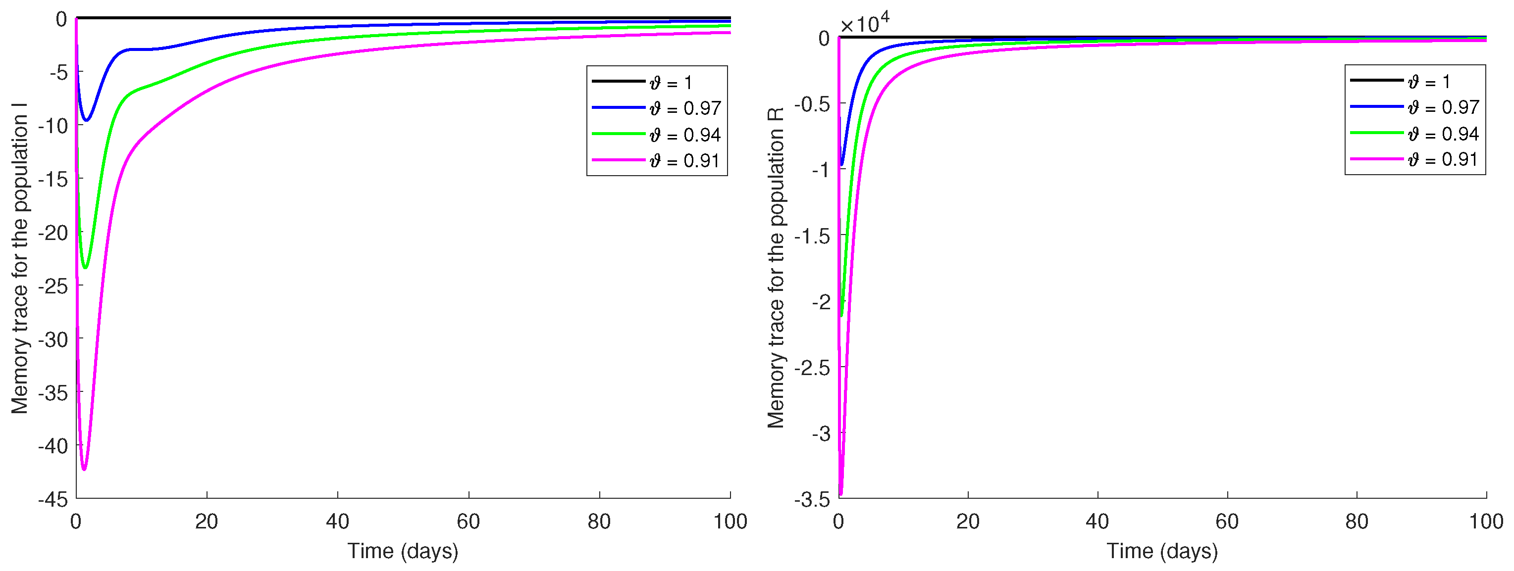
8. Memory Trace and Hereditary Traits

To delve into the behavior of model (4), we utilize the Caputo operator defined in Definition 2, for our analysis. For $\vartheta ,$$0<\vartheta \le 1$ derivative, let the fractional derivative of variable $\mathsf{\Phi }\left(t\right)$ be [45,46,47]

$${}_0^C{D}_t^{\vartheta }\mathsf{\Phi }\left(t\right)=\varphi \left(\mathsf{\Phi }\left(t\right),t\right).$$

(13)

By employing one of the most widely used numerical methods, namely, the L1 scheme [47,48,49], the numerical approximation of the fractional-order derivative (FOD) of $\mathsf{\Phi }\left(t\right)$ is as follows:

$${}_0^C{D}_t^{\vartheta }\mathsf{\Phi }\left(t\right)\approx \frac{{\left(dt\right)}^{-\vartheta }}{\mathsf{\Gamma }\left(2-\vartheta \right)}\left[\sum _{\varrho =0}^{T-1}\left[\mathsf{\Phi }\left(t_{\varrho +1}\right)-\mathsf{\Phi }\left(t_{\varrho }\right)\right]\left[{\left(T-\varrho \right)}^{1-\vartheta }-{\left(T-1-\varrho \right)}^{1-\vartheta }\right]\right].$$

(14)

The L1 scheme stands out as one of the most potent numerical techniques for discretizing the Caputo fractional-order derivative (CFOD) in the temporal domain. While the memory term is also present in various other numerical methods, the L1 scheme offers a more distinct and well-defined representation of this memory integration term. Considering (13) and (14) together, the numerical solution of (13) is as follows:

$$\begin{array}{ccc}\hfill \mathsf{\Phi }\left(t_T\right)& \approx & {}_0^C{D}_t^{\vartheta }\mathsf{\Gamma }\left(2-\vartheta \right)H\left(\mathsf{\Phi }\left(t\right),t\right)+\mathsf{\Phi }\left(t_{T-1}\right)\hfill \\ & & -\left[\sum _{\varrho =0}^{T-2}\left[\mathsf{\Phi }\left(t_{\varrho +1}\right)-\mathsf{\Phi }\left(t_{\varrho }\right)\right]\left[{\left(T-\varrho \right)}^{1-\vartheta }-{\left(T-1-\varrho \right)}^{1-\vartheta }\right]\right].\hfill \end{array}$$

(15)

Hence, the solution of FODEs can be characterized as the disparity between the Markov term and the memory trace. The Markov term is weighted by the Gamma function in the subsequent manner:

$$\mathrm{Markov}\mathrm{term}={}_0^C{D}_t^{\vartheta }\mathsf{\Gamma }\left(2-\vartheta \right)H\left(\mathsf{\Phi }\left(t\right),t\right)+\mathsf{\Phi }\left(t_{T-1}\right).$$

(16)

The memory trace (MT) ($\mathsf{\Phi }$-memory trace since it is related to variable $\mathsf{\Phi }\left(t\right)$) is

$$\mathrm{MT}=\sum _{\varrho =0}^{T-2}\left[\mathsf{\Phi }\left(t_{\varrho +1}\right)-\mathsf{\Phi }\left(t_{\varrho }\right)\right]\left[{\left(T-\varrho \right)}^{1-\vartheta }-{\left(T-1-\varrho \right)}^{1-\vartheta }\right].$$

(17)

The enormous historical evolution of the system is included in the memory trail, which is skillful at merging all previous acts. The memory trace is 0 for any time t when $\vartheta =1$, according to this equation. Time has a significant impact on how memory traces behave. As $\vartheta$ is reduced, the memory trace begins to rise nonlinearly from zero. Therefore, compared to integer systems, fractional-order systems exhibit very different behaviors. Numerical simulations and detailed biological interpretations of memory traces are given in Section 9.

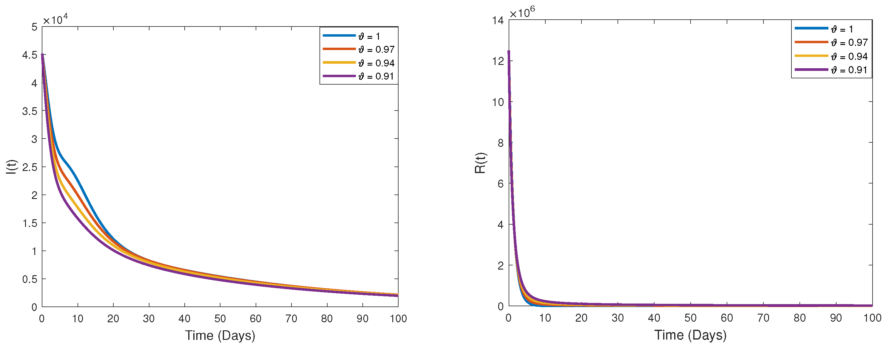
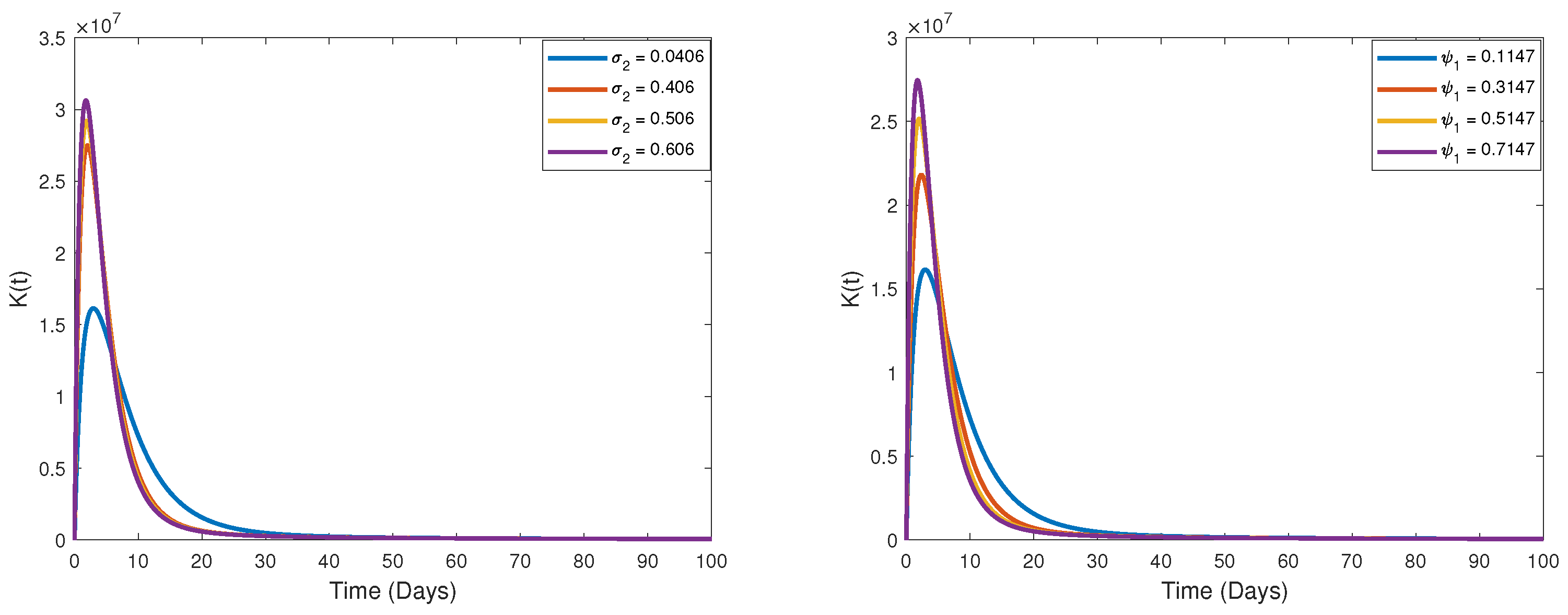
9. Some Numerical Simulations and Biological Interpretations

In this section, the numerical solution of model (4) has been obtained using the Adams–Bashforth–Moulton Predictor-Corrector method. Parameters play a crucial role in regulating the spread of diseases and the potential occurrence of strokes. By employing the parameters listed in

Table 2. Parameter values used for numerical analysis.

Par.	Meaning	Value	Source
${\mathsf{\Lambda }}^{\vartheta }$	Recruitment rate	$2.296187\times {10}^3$	Calculated
${\mu }^{\vartheta }$	The natural death rate	$3.355451\times {10}^{-5}$	Calculated
${\mu }_2^{\vartheta }$	The death rate from stroke	$0.3368$	Fitted
${\beta }_1^{\vartheta }$	Rate of disease transmission through contact with E class	$0.9$	Fitted
${\beta }_2^{\vartheta }$	Rate of disease transmission through contact with I class	$0.8650$	Fitted
${\omega }^{\vartheta }$	The growth rate	$0.2050$	Fitted
$k_1^{\vartheta }$	Level of the fear to be infected with COVID-19	$0.8997$	Fitted
$C^{\vartheta }$	Carrying capacity of S	$6.0660\times {10}^9$	Fitted
${\psi }_1^{\vartheta }$	Rate of susceptible individuals undergoing quarantine	$0.1147$	Fitted
${\psi }_2^{\vartheta }$	Rate of infected individuals without symptoms who have undergone quarantine	$1.3631\times {10}^{-5}$	Fitted
${\psi }_3^{\vartheta }$	Rate of infected individuals exhibiting symptoms	$0.3244$	Fitted
	who have been placed in quarantine		Fitted
$r_1^{\vartheta }$	Recovered rate from COVID-19	$0.1326$	Fitted
${\zeta }^{\vartheta }$	The mortality rate due to complications	$0.00255$	Fitted
${\theta }_1^{\vartheta }$	Screening rate	$0.0163$	Fitted
${\theta }_2^{\vartheta }$	Probability of developing stroke of infected individuals	$0.3999$	Fitted
${\theta }_3^{\vartheta }$	Probability rate of developing stroke of recovered people	$0.4724$	Fitted
${\sigma }_1^{\vartheta }$	probability of having a stroke due to heredity (genetic disorders)	$0.0141$	Fitted
${\sigma }_2^{\vartheta }$	Probability of having a stroke due to a chronic disease such as high	$0.0406$	Fitted
	blood pressure		Fitted
${\tau }^{\vartheta }$	Probability of individuals in S class developing a stroke due to quarantine	$0.8189$	Fitted
${\eta }^{\vartheta }$	The appearance of symptoms of COVID-19 on the infected person	$0.2343$	Fitted

, the changes in each sub-population have been simulated over time for various values of $\vartheta$. Furthermore, considering parameters, graphical representations have been generated for different values of these parameters and for ($\vartheta =0.91$). We have included simulations of the spread of COVID-19 and future predictions of stroke, a long-term side effect of COVID-19. We have aimed to examine the effects of the fear effect, which harms people through different channels, on the dynamics of populations. In this context, we have considered parameters such as screening, the probability of having a stroke, the rate of susceptible individuals who have been in quarantine, fear effect, and screening rate, which are essential in the relationship between COVID-19 and stroke. The dynamic behavior of each sub-population in the proposed COVID-19 and stroke model is illustrated in Figure 3, Figure 4, Figure 5, Figure 6, Figure 7, Figure 8, Figure 9 and Figure 10 for varying values of $\vartheta$ and various parameter values.

In Figure 3, Figure 4 and Figure 5, we have examined the dynamic behavior for each sub-population of the system, taking into account different fractional-order values. Since the disease spread parameters ${\beta }_1=0.9$ and ${\beta }_2=0.8650$ are fairly high, we have seen that the susceptible individuals decrease rapidly until the 30th day, and then almost all of the population S moves to other compartments, especially to the exposed class. So, we have seen that the number of individuals in this class increases until the number of exposed individuals is controlled by screening tests, and then the number in this class decreases thanks to the screening, and the infected class decreases over time. Although the infection rate is high, this decline in the infected class results from individuals who have had a stroke and transitioned to class K for many reasons. Also, it can be seen that the number of recovered individuals decreases over time because there are individuals who have undergone a stroke and passed to the K class (${\theta }_3$) and individuals who have died due to different side effects of COVID-19 after recovery (${\mu }_2$). We have observed that the number of individuals quarantined first increases due to the transition of exposed individuals (${\psi }_2$) to the Q class, and then the number of individuals in this class decreases due to the long-term effect of stroke (${\mu }_2$,$\zeta$). One can see that the individuals in the stroke class increase rapidly and then decrease and stabilize towards zero. Since the individuals in the infected class begin to be detected by screening (${\theta }_1$) and the individuals in the exposed class start to show symptoms of the disease ($\eta$), they go into quarantine. The decrease in the individuals in the K class is due to this process.

If the dynamic behavior of populations is interpreted in terms of fractional-order derivative, as the fractional derivative decreases from 1 to $0.91$, it is simulated that susceptible individuals are in the population. A similar comment can be made for the recovering, quarantined, and stroke classes. However, for exposed and infected individuals, the situation is the opposite, that is, as the fractional derivative value decreases, less exposed and infected individuals are seen. In Figure 6, it can be concluded that the number of class K increases as the (${\sigma }_2$) and (${\psi }_1$) values increase. Here, as the (${\psi }_1$) value increases, the number of people who develop stroke increases, which is an expected result for a biologically well-established model. This result confirms that our model is consistent with reality. In addition, as the (${\psi }_1$) value increases, that is, the number of quarantined individuals from the susceptible class increases, and the number of people who have a stroke due to the adverse effects of quarantine also increases. In Figure 7, by considering the different fear levels $k_1$, we have desired to observe what kind of change would be in class K and I class. The result looks entirely satisfactory indeed. We have observed that the number of people who have had a stroke increases as the level of fear disappears, because as fear decreases, people abandon measures such as individual hygiene measures, quarantine, and vaccination. As a result, more people are exposed to the disease, and therefore the number of people who also face stroke, the post-effect of COVID-19, unfortunately, increases. When we compare Figure 3 and Figure 8, we can see that exposed individuals show a solid increase after the disappearance of the fear effect and susceptible individuals first increase, but then decrease towards zero when the effect of fear begins to take control of this compartment. Finally, in Figure 9, we have desired to investigate the effects of the screening rate on the exposed and infected classes. When we examine Figure 9, an effective decrease in the number of exposed and infected individuals stands out with more PCR tests and an increase in the screening rate. We can conclude that the figures we obtained are quite consistent with the nature of the spread of the disease. From Figure 7, we observe that when the fear rate disappears from the population, the infection spreads further, and the number of people suffering from stroke increases.

Measurement of Memory Trace

As given in detail in Section 8, we have numerically integrated the fractional derivatives using the L1 scheme and the solutions of the FODEs for $S\left(t\right),E\left(t\right),I\left(t\right),R\left(t\right),Q\left(t\right),K\left(t\right),$ which we have described in a similar way as in (14). Thus, the numerical approximation of the fractional-order derivative of $S\left(t\right)$ is:

$${}_0^C{D}_t^{\vartheta }S\left(t\right)\approx \frac{{\left(dt\right)}^{-\vartheta }}{\mathsf{\Gamma }\left(2-\vartheta \right)}\left[\sum _{\varrho =0}^{T-1}\left[S\left(t_{\varrho +1}\right)-S\left(t_{\varrho }\right)\right]\left[{\left(T-\varrho \right)}^{1-\vartheta }-{\left(T-1-\varrho \right)}^{1-\vartheta }\right]\right].$$

(18)

By combining (18) and the first equation of system (4), the numerical solution of Susceptible individuals $S\left(t\right)$ is given by:

$$S\left(t_T\right)\approx \mathrm{Markov}\mathrm{term}\mathrm{of}S\left(t\right)-\mathrm{Memory}\mathrm{trace}\mathrm{of}S\left(t\right),$$

(19)

where

$$\mathrm{Markov}\mathrm{term}={}_0^C{D}_t^{\vartheta }\mathsf{\Gamma }\left(2-\vartheta \right)H\left(S\left(t\right),t\right)+S\left(t_{T-1}\right),$$

(20)

and

$$\mathrm{Memory}\mathrm{trace}=\sum _{\varrho =0}^{T-2}\left[S\left(t_{\varrho +1}\right)-S\left(t_{\varrho }\right)\right]\left[{\left(T-\varrho \right)}^{1-\vartheta }-{\left(T-1-\varrho \right)}^{1-\vartheta }\right].$$

(21)

By following the same steps, the numerical approximations of the fractional-order derivative of $E\left(t\right)$, $I\left(t\right)$, $R\left(t\right)$, $Q\left(t\right)$, $K\left(t\right)$, have been achieved. Numerical assessments have been conducted to visually depict the impact of memory trace on individual sub-populations within the system described by Equation (4) using the outcomes above. Figure 10, Figure 11 and Figure 12 show the effects of memory trace on the dynamics of populations for varied values of fractional-order $\vartheta$. As seen from these Figures, when $\vartheta =1$, the system has no memory effect. As $\vartheta$ decreases from 1 to $0.7$, the impacts of the fractional order and the existence of a memory effect become clear. Memory effect can obtain actual results and forecasting of COVID-19 and stroke interaction. Hence, a memory influence holds significant importance within biological models. Upon a joint examination of Figure 3, Figure 4, Figure 5, Figure 6, Figure 7, Figure 8, Figure 9, Figure 10, Figure 11 and Figure 12, a notable connection between the memory effect and the peak values of the system’s behavior is evident. For example, in Figure 3 and Figure 10, it is seen that the memory trace starts to become negative where exposed individuals for different values of $\vartheta$ begin to decrease after the peak value. When the immune system encounters viruses, a memory response is triggered in biological occurrences, which remains efficacious for a specific duration [50]. Upon analyzing the Figure 10, Figure 11 and Figure 12, it becomes apparent that the memory effect converges to zero beyond a specific timeframe. These findings align with the anticipated outcomes in actual biological processes within the human body. The outcomes derived from the graphical representations indicate that FODEs effectively capture the system’s memory effect, obviating the necessity for additional factors. As is known, fractional-order derivatives are preferred because they have a memory effect. How effectively the memory effect is activated is vital for the system. In analyzing the memory effect graphs, we see that the highest memory effect is for the value of $\vartheta =0.91$. Therefore, the best fractional derivative for this model is $\vartheta =0.91$.

10. Conclusions

Since the onset of COVID-19, many people have either become immune by passing on COVID-19 or become immune by catching the weakened microbe, that is, by being vaccinated. People have started to show some side effects after a certain period after the infection was cleared from their bodies. In this study, we have examined stroke, one of the deadliest long-term side effects of COVID-19, which is common in humans after infection with the virus. In addition, we have aimed to create a more realistic model by including the effect of fear, which negatively affects the growth rate of society and reduces the rate of infection. During the spread of COVID-19, the unproven information heard through media channels, the propaganda made, and the unrealistic scenarios people interpret according to themselves have caused people to fear COVID-19 psychologically. In light of this information, in this study, we have set out to examine the relationship between COVID-19 and stroke and to investigate the effects of fear on the spread of the pandemic. In the introduction part of the study, we have given brief information about COVID-19 and the effect of stroke. Then, we have created a mathematical model that includes the fear effect on the relationship between COVID-19 and stroke. The fact that the predictions of the created model about the future epidemic situation and its side effects are more realistic is closely related to the derivative used in the model. Therefore, in this study, we have proposed a dimensionally compatible model using fractional-order differential equations to incorporate the memory effect, which is vital in the mechanism of epidemic diseases. We have proved its positivity and boundedness to show that the model is biologically meaningful. We also have shown that the solution of the system is unique using the fixed point theorem. We have presented the stability analysis by calculating the equilibrium points of the model. We have calculated the reproduction number and performed a sensitivity analysis. We have performed parameter estimation to calculate our model-specific parameter values using COVID-19 case data for the UK so that our model can more realistically calculate future stroke impact and disease spread. The parameter values used to make forward-looking predictions in most of the mathematical models in the literature are those used in previous studies. This is a factor that limits the accuracy of model predictions. Unlike the studies in the literature, in this study, we have made future predictions for COVID-19 and stroke by using the parameter values we obtained using real data for our model. To demonstrate the advantages of the fractional derivative effect on the system, we have performed detailed analyses of the effects of memory trace and heritable traits. From our findings, we have seen that if the screening rate in the population is increased, more cases can be detected, and stroke development can be prevented. We also have concluded that if the fear in the population is removed, the infection will spread further, and the number of people suffering from a stroke may increase. If the findings obtained from the mathematical modeling studies are paid attention to by experts during disease processes, it can help lead to the effects of the pandemic disappearing in a shorter time and other side effects of COVID-19 being eliminated, such as the stroke effect that we are studying here. Up to the present, a substantial amount of research has been dedicated to the mathematical modeling of COVID-19. Most of these studies are on the spread of COVID-19, and to the best of our knowledge, no studies examining the effects of stroke have been found. In this respect, it is believed that this study, which examines one of the most crucial side effects of COVID-19, will guide future mathematical studies examining post-COVID-19 side effects.

References

1. Koh, J.S.; Hoe, R.H.M.; Chen, G.J.; Goh, Y.; Tan, B.Y.; Yong, M.H.; Hui, A.C.F.; Tu, T.M.; Yong, K.P.; Angon, J.; et al. Low incidence of neurological recurrent side-effects following COVID-19 reimmunization. QJM Int. J. Med. 2023, 116, 221–226. [Google Scholar] [CrossRef] [PubMed]
2. Gill, C.; Cho, T.A. Neurologic complications of COVID-19. CONTINUUM Lifelong Learn. Neurol. 2023, 29, 946–965. [Google Scholar] [CrossRef] [PubMed]
3. Rawat, M.; Ng, C.; Khan, E.; Shah, R.A.; Ashfaq, S.; Bahader, G.A.; Shah, Z.A. Use of mesenchymal stem cell therapy in COVID-19 related strokes. Neural Regen. Res. 2023, 18, 1881. [Google Scholar] [PubMed]
4. Qureshi, A.I.; Baskett, W.I.; Huang, W.; Shyu, D.; Myers, D.; Raju, M.; Lobanova, I.; Suri, M.F.K.; Naqvi, S.H.; French, B.R.; et al. Acute ischemic stroke and COVID-19: An analysis of 27 676 patients. Stroke 2021, 52, 905–912. [Google Scholar] [CrossRef]
5. Rivera, R.; Amudio, C.; Cruz, J.P.; Brunetti, E.; Catalan, P.; Sordo, J.G.; Echeverria, D.; Badilla, L.; Chamorro, A.; Gonzalez, C.; et al. The impact of a two-year long COVID-19 public health restriction program on mechanical thrombectomy outcomes in a stroke network. J. Stroke Cerebrovasc. Dis. 2023, 32, 107138. [Google Scholar] [CrossRef]
6. Nalaini, F.; Salehi Zahabi, S.; Abdoli, M.; Kazemi, E.; Mehrbakhsh, M.; Khaledian, S.; Fatahian, R. COVID-19 and Brain complications in adult and pediatric patients: A review on neuroimaging findings. Cell. Mol. Biomed. Rep. 2023, 3, 212–221. [Google Scholar] [CrossRef]
7. Shama, M.; Mahmood, A.; Mehmood, S.; Zhang, W. Pathological Effects of SARS-CoV-19 Associated With Hematological Abnormalities. Preprints 2023. [Google Scholar] [CrossRef]
8. Mahmoudi, H.; Vardanjani, A.E. Blood Clotting Disorders and Thrombosis: An Important Complication of COVID-19. Acta Microbiol. Bulg. 2023, 39, 12–15. [Google Scholar] [CrossRef]
9. Özköse, F.; Yavuz, M. Investigation of interactions between COVID-19 and diabetes with hereditary traits using real data: A case study in Turkey. Comput. Biol. Med. 2022, 141, 105044. [Google Scholar] [CrossRef]
10. Evirgen, F.; Uçar, S.; Özdemir, N.; Hammouch, Z. System response of an alcoholism model under the effect of immigration via non-singular kernel derivative. Discret. Contin. Dyn. Syst.-S 2021, 14, 2199. [Google Scholar]
11. Naik, P.A.; Zu, J.; Owolabi, K.M. Modeling the mechanics of viral kinetics under immune control during primary infection of HIV-1 with treatment in fractional order. Phys. A Stat. Mech. Its Appl. 2020, 545, 123816. [Google Scholar] [CrossRef]
12. Özköse, F.; Yavuz, M.; Şenel, M.T.; Habbireeh, R. Fractional order modelling of omicron SARS-CoV-2 variant containing heart attack effect using real data from the United Kingdom. Chaos Solitons Fractals 2022, 157, 111954. [Google Scholar] [CrossRef] [PubMed]
13. Öztürk, I.; Özköse, F. Stability analysis of fractional order mathematical model of tumor-immune system interaction. Chaos Solitons Fractals 2020, 133, 109614. [Google Scholar] [CrossRef]
14. Naik, P.A.; Owolabi, K.M.; Zu, J.; Naik MU, D. Modeling the transmission dynamics of COVID-19 pandemic in Caputo type fractional derivative. J. Multiscale Model. 2021, 12, 2150006. [Google Scholar] [CrossRef]
15. Özköse, F.; Şenel, M.T.; Habbireeh, R. Fractional-order mathematical modelling of cancer cells-cancer stem cells-immune system interaction with chemotherapy. Math. Model. Numer. Simul. Appl. 2021, 1, 67–83. [Google Scholar] [CrossRef]
16. Haq, I.U.; Ali, N.; Nisar, K.S. An optimal control strategy and Grünwald-Letnikov finite-difference numerical scheme for the fractional-order COVID-19 model. Math. Model. Numer. Simul. Appl. 2022, 2, 108–116. [Google Scholar] [CrossRef]
17. Allegretti, S.; Bulai, I.M.; Marino, R.; Menandro, M.A.; Parisi, K. Vaccination effect conjoint to fraction of avoided contacts for a Sars-Cov-2 mathematical model. Math. Model. Numer. Simul. Appl. 2021, 1, 56–66. [Google Scholar] [CrossRef]
18. Evirgen, F. Transmission of Nipah virus dynamics under Caputo fractional derivative. J. Comput. Appl. Math. 2023, 418, 114654. [Google Scholar] [CrossRef]
19. Özköse, F.; Yılmaz, S.; Yavuz, M.; Öztürk, İ.; Şenel, M.T.; Bağcı, B.Ş.; Doğan, M.; Önal, Ö. A fractional modeling of tumor–immune system interaction related to Lung cancer with real data. Eur. Phys. J. Plus 2022, 137, 40. [Google Scholar] [CrossRef]
20. Özköse, F.; Habbireeh, R.; Şenel, M.T. A novel fractional order model of SARS-CoV-2 and Cholera disease with real data. J. Comput. Appl. Math. 2023, 423, 114969. [Google Scholar] [CrossRef]
21. Naik, P.A.; Eskandari, Z.; Yavuz, M.; Zu, J. Complex dynamics of a discrete-time Bazykin–Berezovskaya prey-predator model with a strong Allee effect. J. Comput. Appl. Math. 2022, 413, 114401. [Google Scholar] [CrossRef]
22. Sadek, L.; Sadek, O.; Alaoui, H.T.; Abdo, M.S.; Shah, K.; Abdeljawad, T. Fractional order modeling of predicting covid-19 with isolation and vaccination strategies in morocco. CMES-Comput. Model. Eng. Sci. 2023, 136, 1931–1950. [Google Scholar] [CrossRef]
23. Karaagac, B.; Owolabi, K.M.; Pindza, E. A computational technique for the Caputo fractal-fractional diabetes mellitus model without genetic factors. Int. J. Dyn. Control 2023, 11, 2161–2178. [Google Scholar] [CrossRef] [PubMed]
24. Alkahtani, B.S. Mathematical Modeling of COVID-19 Transmission Using a Fractional Order Derivative. Fractal Fract. 2022, 7, 46. [Google Scholar] [CrossRef]
25. Hadi, M.S.; Bilgehan, B. Fractional COVID-19 modeling and analysis on successive optimal control policies. Fractal Fract. 2022, 6, 533. [Google Scholar] [CrossRef]
26. Sun, T.C.; DarAssi, M.H.; Alfwzan, W.F.; Khan, M.A.; Alqahtani, A.S.; Alshahrani, S.S.; Muhammad, T. Mathematical Modeling of COVID-19 with Vaccination Using Fractional Derivative: A Case Study. Fractal Fract. 2023, 7, 234. [Google Scholar] [CrossRef]
27. Dababneh, A.; Djenina, N.; Ouannas, A.; Grassi, G.; Batiha, I.M.; Jebril, I.H. A new incommensurate fractional-order discrete COVID-19 model with vaccinated individuals compartment. Fractal Fract. 2022, 6, 456. [Google Scholar] [CrossRef]
28. Khedr, E.M.; Abdelwarith, A.; Moussa, G.M.; Saber, M. Recombinant tissue plasminogen activator (rTPA) management for first onset acute Ischemic Stroke with COVID-19 and non-COVID-19 patients. J. Stroke Cerebrovasc. Dis. 2023, 32, 107031. [Google Scholar] [CrossRef]
29. Massoud, G.P.; Hazimeh, D.H.; Amin, G.; Mekary, W.; Khabsa, J.; Araji, T.; Fares, S.; Mericskay, M.; Booz, G.W.; Zouein, F.A. Risk of thromboembolic events in non-hospitalized COVID-19 patients: A systematic review. Eur. J. Pharmacol. 2023, 941, 175501. [Google Scholar] [CrossRef]
30. Zuin, M.; Mazzitelli, M.; Rigatelli, G.; Bilato, C.; Cattelan, A.M. Risk of ischemic stroke in patients recovered from COVID-19 infection: A systematic review and meta-analysis. Eur. Stroke J. 2023. [Google Scholar] [CrossRef]
31. Van Dusen, R.A.; Abernethy, K.; Chaudhary, N.; Paudyal, V.; Kurmi, O. Association of the COVID-19 pandemic on stroke admissions and treatment globally: A systematic review. BMJ Open 2023, 13, e062734. [Google Scholar] [CrossRef] [PubMed]
32. Ferrone, S.R.; Sanmartin, M.X.; Ohara, J.; Jimenez, J.C.; Feizullayeva, C.; Lodato, Z.; Shahsavarani, S.; Lacher, G.; Demissie, S.; Vialet, J.M.; et al. Acute ischemic stroke outcomes in patients with COVID-19: A systematic review and meta-analysis. J. NeuroInterventional Surg. 2023. [Google Scholar] [CrossRef] [PubMed]
33. Sasmal, S.K. Population dynamics with multiple Allee effects induced by fear factors—A mathematical study on prey-predator interactions. Appl. Math. Model. 2018, 64, 1–14. [Google Scholar] [CrossRef]
34. Podlubny, I. Fractional Differential Equations; Academic Press: New York, NY, USA, 1999. [Google Scholar]
35. Ghaziani, R.K.; Alidousti, J.; Eshkaftaki, A.B. Stability and dynamics of a fractional order Leslie–Gower prey–predator model. Appl. Math. Model. 2016, 40, 2075–2086. [Google Scholar] [CrossRef]
36. Petráš, I. Fractional-Order Nonlinear Systems: Modeling, Analysis and Simulation; Springer Science & Business Media: Berlin/Heidelberg, Germany, 2011. [Google Scholar]
37. Lin, W. Global existence theory and chaos control of fractional differential equations. J. Math. Anal. Appl. 2007, 332, 709–726. [Google Scholar] [CrossRef]
38. Odibat, Z.M.; Shawagfeh, N.T. Generalized Taylor’s formula. Appl. Math. Comput. 2007, 186, 286–293. [Google Scholar] [CrossRef]
39. Odibat, Z.; Baleanu, D. Numerical simulation of initial value problems with generalized Caputo-type fractional derivatives. Appl. Numer. Math. 2020, 156, 94–105. [Google Scholar] [CrossRef]
40. Van den Driessche, P.; Watmough, J. Reproduction numbers and sub-threshold endemic equilibria for compartmental models of disease transmission. Math. Biosci. 2002, 180, 29–48. [Google Scholar] [CrossRef]
41. Diekmann, O.; Heesterbeek, J.A.P.; Roberts, M.G. The construction of next-generation matrices for compartmental epidemic models. J. R. Soc. Interface 2010, 7, 873–885. [Google Scholar] [CrossRef]
42. Breda, D.; Florian, F.; Ripoll, J.; Vermiglio, R. Efficient numerical computation of the basic reproduction number for structured populations. J. Comput. Appl. Math. 2021, 384, 113165. [Google Scholar] [CrossRef]
43. Breda, D.; Kuniya, T.; Ripoll, J.; Vermiglio, R. Collocation of next-generation operators for computing the basic reproduction number of structured populations. J. Sci. Comput. 2020, 85, 1–33. [Google Scholar] [CrossRef]
44. Chitnis, N.; Hyman, J.M.; Cushing, J.M. Determining important parameters in the spread of malaria through the sensitivity analysis of a mathematical model. Bull. Math. Biol. 2008, 70, 1272. [Google Scholar] [CrossRef]
45. Vargas-De-León, C. Volterra-type Lyapunov functions for fractional-order epidemic systems. Commun. Nonlinear Sci. Numer. Simul. 2015, 24, 75–85. [Google Scholar] [CrossRef]
46. Naik, P.A.; Yavuz, M.; Zu, J. The role of prostitution on HIV transmission with memory: A modeling approach. Alex. Eng. J. 2020, 59, 2513–2531. [Google Scholar] [CrossRef]
47. Jin, B.; Lazarov, R.; Zhou, Z. An analysis of the L1 scheme for the subdiffusion equation with nonsmooth data. IMA J. Numer. Anal. 2016, 36, 197–221. [Google Scholar] [CrossRef]
48. Du, M.; Wang, Z. Correcting the initialization of models with fractional derivatives via history-dependent conditions. Acta Mech. Sin. 2016, 32, 320–325. [Google Scholar] [CrossRef]
49. Magin, R.L. Fractional Calculus in Bioengineering; Begell House Publishers Redding: Redding, CT, USA, 2006. [Google Scholar]
50. van Baarle, D.; Tsegaye, A.; Miedema, F.; Akbar, A. Significance of senescence for virus-specific memory T cell responses: Rapid ageing during chronic stimulation of the immune system. Immunol. Lett. 2005, 97, 19–29. [Google Scholar] [CrossRef]
Figure 1. The state variables and transitions.
Fractalfract 07 00719 g001
Figure 2. Reported real cases of COVID-19 in UK and the best-fit curve of model.
Fractalfract 07 00719 g002
Figure 3. Change of Susceptible and Exposed individuals over time for various ϑ values.
Fractalfract 07 00719 g003
Figure 4. Change of I and R class over time for various ϑ values.
Fractalfract 07 00719 g004
Figure 5. Change of Q and K class over time for various ϑ values.
Fractalfract 07 00719 g005
Figure 6. Change of K class over time for some σ 2 and ψ 1 values.
Fractalfract 07 00719 g006
Figure 7. Change of people in I and K class over time for various k 1 values.
Fractalfract 07 00719 g007
Figure 8. Change of people in S and E class over time for k 1 = 0 .
Fractalfract 07 00719 g008
Figure 9. Change of E and I class over time for various θ 1 values.
Fractalfract 07 00719 g009
Figure 10. The influence of memory trace on Susceptible and Exposed individuals (right) for different ϑ values.
Fractalfract 07 00719 g010
Figure 11. The influence of memory trace on Infected (left) and Recovered Individuals (right) for different ϑ values.
Fractalfract 07 00719 g011
Figure 12. The influence of memory trace on people in Quarantine (left) and having Stroke (right) for different ϑ values.
Fractalfract 07 00719 g012