Article

The Importance of Non-Systemically Important Banks—A Network-Based Analysis for China’s Banking System

Business School, China University of Political Science and Law, Haidian, Beijing 100088, China
Fractal Fract. 2023, 7(10), 735; https://doi.org/10.3390/fractalfract7100735
Submission received: 25 July 2023 / Revised: 9 August 2023 / Accepted: 12 September 2023 / Published: 6 October 2023

Abstract

:
There is important theoretical and practical significance to scientifically identifying the systemic importance of banks for effectively preventing and controlling systemic risks in the banking system. Prevalent identification methods are biased because they only pay attention to measuring the systemic risk contribution of individual banks to the whole system in order to determine that bank’s systemic importance. Less attention is paid to the cascade effects of risk spillover among banks. This study proposes a novel method for measuring the cascade effects of risk spillover of banks and their contributions to systemic risks by building up a conditional tail risk network of China’s banking system. Different from previous analyses of systemic risks based on the identification and risk measurement of systemically important banks (SIBs), this paper focuses on analyzing the risk spillover effects of non-SIBs and their contributions to systemic risks by building up a conditional tail risk network of China’s banking system. Our empirical results show that some non-SIBs in China are more vulnerable to the shocks of systemic risk than SIBs, and that they are more likely to act as key intermediaries to transmit risk to SIBs, thereby triggering systemic risk. In view of this, we propose to identify key non-SIBs according to their risk spillover intensity because they are also systemically important. The market regulators not only need to pay attention to SIBs that are too big to fail, but also treat seriously the key intermediaries of “risk spillover too strong to fail” in the network in order to ensure the stability of the banking system.

1. Introduction

After the 2008 financial crisis, strengthening the supervision of systemically important financial institutions (SIFIs) has become one of the core issues in the financial reform of various countries. The identification of SIFIs works under the premise of supervision and is also the focus of regulatory reform. A useful definition of SIFIs was advanced by Federal Reserve Governor Daniel Tarullo, who said that “Financial institutions are systemically important if the failure of the firm to meet its obligations to creditors and customers would have significant adverse consequences for the financial system and the broader economy.” Although the definition of SIFIs is clear, the methods of identification are not consistent. International financial regulators and monetary authorities judge SIFIs mainly based on the indicator-based method. The Macroprudential Group (MPG) of the Basel Committee on Banking Supervision (BCBS) is responsible for developing indicators and methods for identifying SIFIs. MPG published a more detailed indicator system on 11 October 2010 [1], and improved it again in November 2022. The indicators usually focus on describing the scale, the correlation, and the negative externalities of SIFIs. Scholars often use the market-based method to determine the systemic importance of individual financial institutions. The existing market-based methods mainly include the marginal expected Shortfall (MES) [2,3], Shapley Value [4], CoVaR [5], and Extreme Value [6]. These methods are essentially based on the underlying theoretical position that the bigger a financial institution is, the greater the breadth of products it provides and the larger scale transactions it involves, the higher risk contribution to the financial system it has. These prevalent identification methods are biased because less attention is paid to the cascade effects of risk spillover among banks. With the development of the banking industry, the scale of interbank business has been expanding, and it can be argued that the linkages between banks are becoming stronger. Without taking into account the cascade effects of risk spillover between banks, the identification of such SIBs would be inaccurate.
In the case of China’s banking system, the People’s Bank of China (PBC) and the China Banking and Insurance Regulatory Commission (CBIRC) designated a total of 19 banks as systemically important banks (SIBs) in 2022, with a focus to deliver additional regulation to those banks. These 19 SIBs consist of six state-owned commercial banks (Industrial and Commercial Bank of China, Bank of China, China Construction Bank, Postal Savings Bank of China, Bank of Communications, and Agricultural Bank of China), nine joint-stock commercial banks (China Minsheng Bank, China Everbright Bank, Pingan Bank, Huaxia Bank, China Guangfa Bank, China CITIC Bank, and Shanghai Pudong Development Bank, China Merchants Bank, and Industrial Bank), and four city commercial banks (Bank of Ningbo, Bank of Jiangsu, Bank of Shanghai, and Bank of Beijing) (PBC press release, 9 September 2022). Each SIB’s total assets exceed 1500 billion yuan. However, it is found that the expectation of SIBs being “too big to fail” actually reduces the probability of them causing systemic risks. Additionally, the non-SIBs, some small-sized banks, with total assets of about 500 billion yuan or less, often have a greater probability of failure, such as the recent bankruptcy of Baoshang Bank, Shantou Commercial Bank, Liaoyang Rural Commercial Bank, and Liaoning Taizihe Rural Bank, causing a considerable degree of public panic. Are the failures of non-SIBs or small-sized banks irrelevant? Are they really going to have no effect on systemic risk of the banking sector? This is a practical problem that urgently needs to be answered.
In this paper, we propose a novel method, which is the algorithm-based identification of the risk spillover effects of banks, in order to judge the systemic importance of banks by building up a conditional tail risk network of China’s banking system. We conduct empirical analysis by using the data of stock prices of 54 listed banks in the Chinese securities market with a sample period from June 2021 to June 2023 and we adopt the method proposed in this paper to rank the systemic importance of these banks. Our empirical results shows that some non-SIBs in China are more vulnerable to the shocks of systemic risk than SIBs, and that they are more likely to act as key intermediaries for the transmission of risk to SIBs, in turn triggering systemic risk. In view of this, we propose to identify key non-SIBs according to their risk spillover intensity because they are also systemically important. The market regulators not only need to pay attention to SIBs that are too big to fail, but also seriously consider the key intermediaries of “risk spillover too strong to fail” in the network in order to ensure the stability of the banking system.
The remaining sections of this paper are as follows. In Section 2, we review the prevalent modeling methods of risk spillover effects among academia. In Section 3, we introduce all the technical methods used in this paper, including the GCoVaR method and the fitting technique. In Section 4, we present the empirical analysis of China’s banking system and a robustness test for GCoVaR method. Section 5 concludes.

2. Literature Review

The financial system can be regarded as a financial network. The extreme risks of individual financial institutions would lead to the deterioration of the overall risk of the financial system through network links, which is the main manifestation of systemic financial risks. Network modeling is often used to explore such financial risk contagion. In these network model institutions are nodes, and the connecting edges represent the business relations between institutions. As an interdisciplinary technology, the complex network method provides a theoretical framework in order to help people better understand the internal structure and dynamic behavior of complex systems (Neveu, 2018). By constructing a network, researchers can not only analyze the network structure and characteristics from the perspective of the system, but also analyze the characteristics of important nodes in the system. The construction of a network requires a connection matrix used to express the risk contagion and information spillover among nodes. The data used for the calculation of connection matrix can be roughly divided into two categories. One is inter-institutions’ offered credit or capital flow data. This is based on the specific business connections between institutions [7,8,9,10]. The other is market data, such as stock prices or credit default swap (CDS) prices of the institutions [11,12,13]. Based on the increasing availability of data, stock market data is being more and more widely used. The market data of financial institutions could reflect investors’ sentiment and is real-time and forward-looking; it provides an immediate and transparent measure for studying systemic financial risks [14,15].
The traditional methods used for the calculation of connection matrixes are mainly the correlation coefficient method [16], probabilistic analysis [17], and the error correction model [18]. Because these traditional methods are unable to describe the nonlinearity, dynamics, and asymmetry of risk spillovers, Conditional Value at Risk (CoVaR), introduced by Adrian and Brunnermeier [5], a method that quantifies the amount of tail risk an investment portfolio, has been widely used in recent years. Reboredo and Ugolini [19] analyzed the systemic risks of the European sovereign debt market by using CoVaR method and believed that this method could better identify the changes of risk spillovers before and after the Greek debt crisis. Reboredo and Rivera-Castro [20] verified the asymmetric risk spillover effect of the exchange rates between the Euro and the US Dollar on major global emerging stock markets by calculating their CoVaR. Warshaw [21] proved the effectiveness of CoVaR method by measuring the extreme risk spillover effect of the North American equity market and its changes before and after the subprime crisis.
However, Lopez-Espinosa et al. [22] found empirically that the original CoVaR model, based on the normal hypothesis, underestimated the systemic financial risks of the U.S. listed banks. In response, they introduced asymmetric terms to improve the quantile regression method of CoVaR. Girardi and Ergun [23] also pointed out that CoVaR would underestimate risks under extreme conditions by studying a network consisted of 74 listed banks in the United States, and then proposed an improved generalized conditional value at risk (GCoVaR) method. Their empirical analysis verified that GCoVaR could improve the stability of the measurements obtained. GCoVaR could consider more distress events within the tail region, which would more accurately reflect the characteristics of “volatility clustering, thick tail and nonlinear correlation” of financial markets. Torri et al. [24] believe that using GCoVaR to measure the risk spillover effect would not only help investors to manage portfolio risks, but also help market regulators to carry out dynamic monitoring of financial risks.
As for financial risk contagion, previous studies have mostly focused on the identification and risk measurement of systemically important financial institutions [14,15], and explore ways and tools for preventing and controlling the financial systemic risk based on systemically important financial institutions [25,26]. However, the financial system is made up of systemically important financial institutions and non-systemically important financial institutions, and they both have impacts on the formation and amplification of financial systemic risks. Mistrulli [27] stated that systemic risk can be characterized as a negative pecuniary externality exerted by financial institutions, and that any institution’s risk exposure may evolve into a systemic risk through its interconnectedness within the financial system. Scholars engaged in correlation research believe that the stronger the correlation among institutions, the greater the effect of risk contagion, and more easily to induce systemic risks. However, some scholars suggest that correlation is an effective way to disperse systemic risks [28]. Georg [29]pointed out that the degree of connection between institutions and the level of risk contagion have a non-monotonic relationship. A higher degree of connection between institutions is conducive to risk diversification when the connection level is low, but when it exceeds a certain threshold, the risk of contagion would increase rapidly and could lead to large-scale collapse of institutions. Therefore, some scholars propose that it should pay attention not only to institutions that are “too big to fail”, but also to banks that are “too connected to fail” in order to prevent and control systemic risk [30,31].
It can be seen above that most studies in this area are based on the systemically important financial institutions in order to explore ways to identify and mitigate systemic risks. Less research has been done specifically on non-systemically important financial institutions. The mechanism of risk transfer between SIBs and non-SIBs has not been well understood. In addition, compared with systemically important financial institutions, the number of non-systemically important financial institutions is large, which is difficult to focus on in the research process. In view of this, based on the perspective of risk contagion, this paper measures the risk spillover effect among listed banks in China using the GCoVaR method and Copula technology, and explores the role of non-SIBs in the formation and accumulation of systemic risks in the banking sector. Different from the conventional mode of analyzing systemic risks based on SIBs in previous studies, we focus on analyzing the role and influence of non-SIBs in China’s banking system from two aspects–the risk contribution of non-SIBs to systemic risk and the risk impact of the whole banking system on non-SIBs–in order to test whether or not non-SIBs are unimportant.

3. Methodology

Risk spillover is the transmission of risk from one institution (industry or market) to another institution (industry or market). This is because financial data, in reality, is usually not normally distributed, and presents a “peak and thick tail” distribution. The traditional parametric regression method based on mean estimation cannot accurately reflect the relationship between different parts of the overall distribution. We consider using the tail dependence relationship of stock price of related banks to establish connection matrix of the network of China’s banking system, and the GCoVaR approach to identify risks that are “extra” parts due to the presence of other banks in distress.

3.1. GCoVaR Model

The traditional method measuring the risk, value at risk (VaR), refers to the maximum possible loss of a certain bank in a certain period in the future under a certain confidence level. Let  R i represent the return rate of bank i, then the  V a R i of  R i at a significance level α can be expressed as:
P ( R i V a R i ) = α ,
VaR can only measure the risk of a single bank. Based on this value, conditional value at risk (CoVaR) proposed by Adrian and Brunnermeier [5] can be used to measure the risk spillover between different banks. Let  R j represents the return rate of bank j, under the condition of  R i having an extreme loss  V a R i , at the confidence level of β, the extreme loss of  R j would be  C o V a R j | i , the mathematical expression is:
P ( R j C o V a R j | i | R i = V a R i ) = β ,
According to Girardi and Ergun [23], the  G C o V a R j | i is the VaR of bank j conditional on bank i being at most at its VaR ( R i V a R i ) as opposed to being exactly at its VaR ( R i = V a R i ).
P ( R j G C o V a R j | i | R i V a R i ) = β ,
This change allows us to consider more severe distress events of bank i that are farther along the tail (below its VaR) so as to more accurately reflect the characteristics of financial time series: “volatility agglomeration, thick tail and nonlinear correlation”. This change also improves the consistency of risk measurement with respect to the dependence parameter.
  • The risk spillover between bank i and j
We define the systemic risk contribution of a bank as the change from its GCoVaR in its benchmark state (defined as a one-standard deviation event) to its GCoVaR under financial distress, so we can get the risk spillover effect of bank i to bank j when bank i in extreme distress:
Δ G C o V a R j | i = G C o V a R j | i M C o V a R j | i ,
where  M C o V a R j | i represent the financial distress in GCoVaR of bank j when bank i at a normal state (i.e., α = 0.5), it meets:
P ( R j M C o V a R j | i | R i 0.5 ) = β ,
Define risk spillover intensity γ, which is the change rate of GCoVaR with respect to MCoVaR:
γ j | i = G C o V a R j | i M C o V a R j | i M C o V a R j | i ,
The risk spillover effect is usually bidirectional. Bank i may spill risks to bank j, and conversely, bank j may spill risks to bank i. In addition to effectively measuring the extreme risk spillover effect, another advantage of GCoVaR method is that it can measure the asymmetry of this effect. Let  Δ G C o V a R i | j represents the risk spillover of bank j on bank i, the calculation formula can be similarly derived.
2.
The risk contribution of bank i to the financial system
Let GCoVaRindex|i stands for the generalized conditional value at risk of the financial system suffering from the impact of bank i in distress. Using the same logic above, we have
P ( R i n d e x G C o V a R i n d e x | i | R i V a R i ) = β ,
  Δ G C o V a R i n d e x | i = G C o V a R i n d e x | i M C o V a R i n d e x | i ,
γ i n d e x | i = G C o V a R i n d e x | i M C o V a R i n d e x | i M C o V a R i n d e x | i ,
3.
The risk spillover of bank i suffered from financial system
Let GCoVaRi|index stands for the generalized conditional value at risk of bank i when the whole financial system is in trouble. VaRindex is unconditional value at risk of the financial system. It represents the risk level of the financial system as a whole, we have:
P ( R j G C o V a R i | i n d e x | R t i n d e x V a R α , t i n d e x ) = β ,
Δ G C o V a R i | i n d e x = G C o V a R i | i n d e x M C o V a R i | i n d e x ,
γ i | i n d e x = G C o V a R i | i n d e x M C o V a R i | i n d e x M C o V a R i | i n d e x ,

3.2. To Measure GCoVaR Based on Copula Model

According to the definition of conditional probability, Equation (3) can be transformed into:
P ( R j C o V a R j | i ,   R i V a R i ) = β · P ( R i V a R i ) = α β ,
It can be seen from Equation (13) that the joint distribution of  R j and  R i need to be known in order to calculate GCoVaR. A convenient method is to use Copula function to construct joint distribution of multivariate random variables. Copula function is also known as link function, which can describe the tail correlation between random variables. According to Sklar’s theorem, we can construct the joint distribution of random variables by treating each one-dimensional distribution of multiple random variables as marginal distribution. Equation (13) can be written in the following Copula form:
c ( F j ( G C o V a R j | i ) ,   F i ( V a R i ) ) = α β ,
where, c(∙,∙) is the Copula function, and  F i ( · ) and  F j ( · ) are the edge distribution functions of  R i and  R j , respectively. According to the definition of VaR, Equation (1) means,
F i ( V a R i ) = α ,
According to Equations (3) and (14), given the marginal distribution, the form of Copula connect function, and the confidence level of α and β, the  G C o V a R j | i can be solved. Setting the α to 0.5, the same two equations above can be used to solve for the  M C o V a R j | i ; According to Equations (4)–(6), the  Δ G C o V a R j | i and  γ j | i could be calculated to measure the risk spillover effect of bank i on j. Repeating the above process, we can obtain  Δ G C o V a R i | j and  γ i | j , the risk spillover effect of bank j on i. The marginal distribution, time-varying Copula function and its parameter estimation methods are shown in Appendix B.

4. Empirical Analysis

4.1. Sample Selection

In this paper, 54 listed banks are selected to construct the banking system of China. The selected banks and their total assets are shown in Appendix A. The sample period is from 1 June 2021 to 30 June 2023. The selection of sample periods is mainly based on the consideration that they have normal transaction data in the sample period, so as to make the calculation of value at risk meaningful. All sample data are collected from the Wind Database (https://www.wind.com.cn/portal/zh/WFT/index.html accessed on 30 June 2023). Additionally, R language software (R-4.0.2) is used for Copula function regression analysis, and Python 3.5.0 (Networkx 3.1) is used for mapping.
In Figure 1, the size of the nodes are measured by the weighted degree centrality of nodes. The larger the node’s size is, the nearer to the center the node tends to be in the network.

4.2. Risk Spillover Effect Analysis

4.2.1. The Risk Spillover Effect between Banks

The risk spillover effect of bank i on j can be calculated by Equations (3)–(6) when bank i is in distress. Considering that smaller quantile values are often used in risk management to capture the characteristics of the peak and fat tail of financial time series, here we choose β = 0.025. Since our research sample includes 54 banks, there should be 1431 different combinations of banks, and there are 1431 risk spillover intensity measures. Table 1 gives the results, which are listed in descending order of γj|i. Only the top 30 are listed in order to save space.
Table 1 shows that:
First, given bank i and j, the level of GCoVaRj|i is larger than that of MCoVaRj|i. This suggests that when one bank gets into trouble, other banks are exposed to more than their own level of risk. As shown in line No. 1 of Table 1, MCoVaRCMBC|CDB = 8.14, GCoVaRCMBC|CDB = 12.36. Obviously, MCoVaRCMBC|CDB < GCoVaRCMBC|CDB.
Second, GCoVaRj|i ≠ GCoVaRi|j. The reason is that for GCoVaRj|I, the conditional event is bank i in distress, while for GCoVaRi|j, the conditional event is bank j in distress. Different directions of risk shocks might have different effects. Take the Table 1 line No. 2 as an example: when BSZ is in distress, NJB would suffer risk impact of GCoVaRNJB|BSZ = 11.26; when NJB is in distress, as shown in line No. 27 of Table 1, BSZ would suffer risk impact of GCoVaRBSZ|NJB = 11.71; as such, apparently, GCoVaRBSZ|NJB ≠ GCoVaRNJB|BSZ
Third, from Table 1 we can find that the non-SIBs’ risk spillover should never be underestimated. For the first 30 strongest risk spillover effects, sixteen of them are from non-SIB to non-SIB, eight are from non-SIB to SIBs, two are from SIB to SIB, and four from SIB to non-SIB. The eight non-SIBs who transmit risk to SIBs should be paid special attention. We take CDB, a city commercial bank among the non-SIBs, as an example in order to analyze its risk spillover performance and determine who has the greatest risk impact on SIB. Table 2 shows the banks affected by the risk impact of CDB and the banks from which CDB receives risk spillover. As a relatively small sized city commercial bank with total assets of 652.43 billion yuan, its risk spillovers mainly transmit to other related city commercial banks (CHB, GZB, WHCB, BQD), joint-stock commercial banks (CMBC, CIB, CBH, PAB, HXB), and state-owned commercial banks (BOC, BOCOM), and it received risk spillover from other related city commercial banks (WHCB, SHB, CHB, JZB, JJB, JSB, HSB, SJB), rural commercial banks (CRC, JRC, JSR, JRCB, JZR), and joint-stock commercial banks (CMBC).
For the rural commercial banks among non-SIBs, we take CRC as an example to analyze its risk spillover performance. As a rural commercial bank, CRC has the highest risk spillover on other banks. Table 3 shows the banks impacted by CRC’s risk spillover and the banks from which CRC receives risk spillover. We can see that its risk spillover mainly affects related city commercial banks (CHB, WHCB, CDB, JZB, JSB, GSB, NBB) and rural commercial banks (JSR, ZRCB, JZR, GRCB), while it mainly receives risks from other rural commercial banks (JSR, GRCB, JZR, JRC).
Fourth, SIBs mainly are state-owned commercial banks and joint-stock commercial banks. For the state-owned commercial banks among the SIBs, we take CCB as an example. Table 4 shows the banks affected by CCB’s risk spillover when it is in distress and the banks impacting CCB by risk spillover. All of them are joint-stock commercial banks and city commercial banks, except ABC, which ranks No. 1 in risk outflow column and ranks No. 12 in risk inflow column. It should be noted that the same is true for other state-owned commercial banks’ spillover relations, indicating that the six state-owned commercial banks are relatively independent from each other and the risk spillover intensity between them is generally small.
For the joint-stock commercial bank among the SIBs, we take CMBC as an example. Table 5 shows the banks affected by CMBC’s risk spillover when it is in distress and the banks impacting CMBC by risk spillover. We can see that its risk spillover mainly affects the related city commercial banks (GSB, CDB, SHB, NJB) and joint-stock and state-owned commercial banks (ZSB, CBH, CIB, CCB, ABC), while it mainly receives risks from other joint-stock commercial banks (SPDB, CIB) and city commercial banks (CDB, JSB, SHB, XAB, CHB, GYB, JSBK, ZYB, BSZ, HRB, HSB, XMIB, CSB). It should be noted that the same is true for other joint-stock commercial banks’ spillover relations.
The above analysis shows that the risk spillover of China’s banking system not only has characteristics of contagious diffusion within the same level regional or local banks, but also has a characteristic of hierarchical diffusion, that is, the diffusion from rural commercial banks to city commercial banks to joint-stock commercial banks and state-owned commercial banks. The coordination and cooperation between national banks’ branches and local banks often play a key role in such hierarchical diffusion. Non-SIBs are intended to act as risk transmission intermediaries and transmit risks to SIBs, further inducing systemic risks of the whole banking sector.

4.2.2. The Risk Spillover Effect from Bank to Banking System

Based on Formulas (7)–(9), the individual bank’s risk contribution to the entire banking system γindex|i are calculated when the individual bank is in distress. The calculated results are shown in Figure 2.
As it can be seen from Figure 2, the contributions of banks to systemic risk do not fully positively correspond to their total assets. e.g., the top three biggest China’s banks based on total assets in 2022 (ICBC (with total assets 33,345.10 billion yuan), CCB (28,132.25 billion yuan) and ABC (27,205.05 billion yuan)) have γindex|i 45.88%, 34.7%, 56%, respectively, which are 6th, 17th, and 4th in the ranking of 54 banks’ contribution to systemic risk, respectively. While the banks with the top three highest values of γindex|i (CMBC (γindex|CMBC = 75%), NJB (69%) and CEB (63%)) have only 6950.23, 1517.08, and 5368.11 billion yuan in total assets, respectively, which rank 11th, 20th, and 13th among total assets, respectively.

4.2.3. The Risk Spillover Effect from Banking System to Individual Banks

Figure 3 shows the calculated results of γi|index based on Equations (10)–(12). It can be seen that the strongest shocks from the banking system hit non-SIBs rather than SIBs. Non-SIBs are subject to relatively strong impact by the systematic risks. We find CDB, ranking second, is not only subject to significant systemic risk impact, but also transmits a strong risk spillover to SIBs (see Table 2). If a non-SIB is more vulnerable to the shocks of systemic risk, and it is more likely to transmit risk to SIBs, it will be systemically important because its risk transmission could increases the accumulation of systemic risk greatly. We call it a key intermediary or a key non-SIB.
As is shown in Figure 3, there is only one SIB -SHB, its γi|index is at the upstream level, ranks the eighth; nine SIBs’ γi|index are at the middle level, γCEB|index ranks the 11th, γCITIC|index, γBOCOM|index, γCMBC|index, γHXB|index, γBOB|index, γSPDB|index, γNBB|index and γJSB|index ranks the 21th, 23th to 28th, and 30th; other nine SIBs’ γi|index are at the lower level; the six state-owned commercial banks are almost unaffected by systemic risks. That indicates that although the transaction scale and scope of banks are the basic determining factors of systemic importance, the inter-bank correlation and its risk spillover characteristics in the network have a more structural influence on their systemic importance ranking in the financial system.

4.3. A Robustness Test

In order to test the reliability of the GCoVaR method used in this paper, a robustness test is conducted by using the adjacency information entropy method. This method is also a network analysis approach and works well for investigating the direct and indirect connection effects in the network, which helps to reflect the full view of systemic importance of financial institutions in the financial system (Jamil and Yukongdi, 2020; Allen and Gale, 2000 [32,33]). The basic idea of the adjacency information entropy method is that it regards each bank as a node in the banking network and computes the adjacency information entropy of every node by calculating its degree of adjacency. Subsequently, the importance of each node in the banking network is identified in line with the size of adjacency information entropy. We calculate the adjacency information entropy H of each bank for the 54 public offered banks by referring to Equations (A8)–(A13) in Appendix C (For simplicity, we assume λ = 0.5, means pay equal attention to the in-degree and out-degree). Then, rankings of banks are obtained and demonstrated in Figure 4. Please refer to Appendix C for specific calculation procedures.
The ranking of banks in Figure 4 are basically consistent with that in Figure 2 in terms of the bank types. For some small and medium-sized city commercial banks e.g., NJB, JSB, NBB, their risk features are much higher than those of SIBs. It shows that the GCoVaR method used in this paper is robust and can provide useful measurement of the non-SIBs’ risk spillover effects and rankings of systemically risky banks.

5. Conclusions

In the banking system, banks are closely connected and interact with each other, thus forming a financial network. Since the individual extreme risks of banks could be reflected by tail risks, it is necessary to scientifically reveal the correlation mechanism of banks’ tail risks and its heterogeneous characteristics. There is important theoretical and practical significance to scientifically identifying the systemic importance of banks for effectively preventing and controlling systemic risks of banking system.
In this paper, the GCoVaR method is used to measure the risk spillover intensity between any two banks of China’s banking system. The results show that:
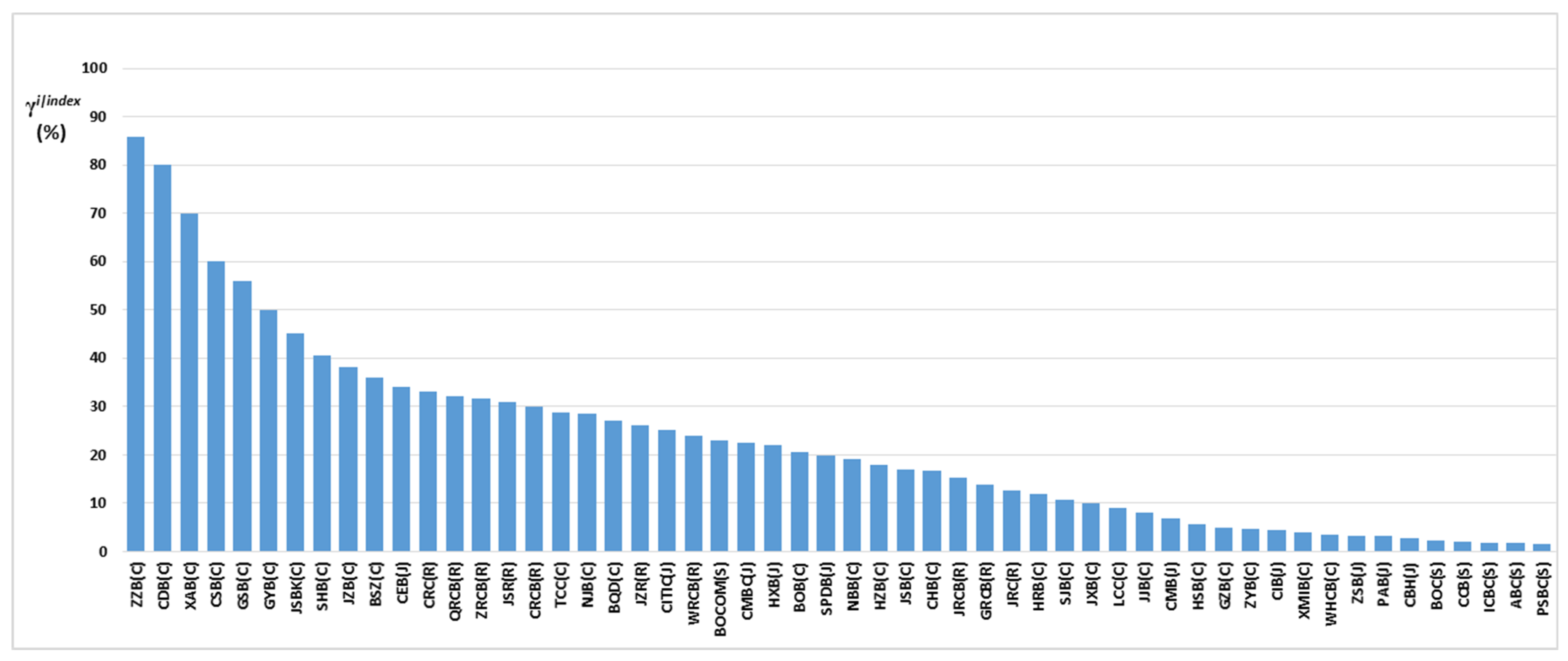
  • Compared with SIBs, the non-SIBs are weaker to resist systemic risk impact. Figure 3 ranks the individual banks based on the intensity of systemic risk impact in descending order. Most of the SIBs have a stronger ability to withstand the impact of systemic risks in the banking sector, especially the state-owned SIBs are almost unaffected by systemic risk in terms of γi|index. On the contrary, non-SIBs are mostly severely affected by systemic risks.
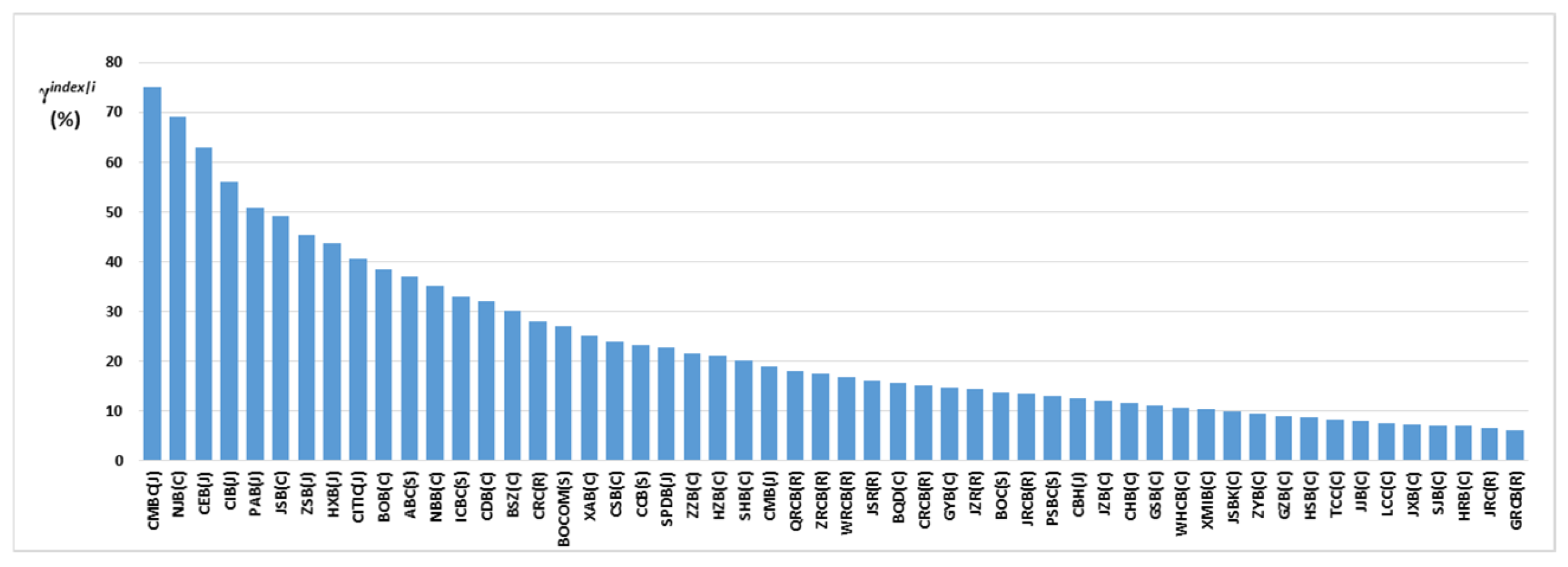
  • China’s banking risk spillover has characteristics of hierarchical diffusion from rural commercial banks to city commercial banks to joint-stock commercial banks and state-owned commercial banks. It is mainly from non- SIBs that SIBs receive large risk impacts. It can be seen that in China’s banking system, some non-SIBs, especially some city commercial banks, are more vulnerable to the shocks of systemic risk than SIBs, and they are more likely to act as key intermediaries to transmit risk to SIBs, in turn to trigger systemic risk. So, if the risk prevention and control efforts for the key intermediary are insufficient, the seemingly small risk shocks are likely to be transmitted from non-SIBs to SIBs, thus generating the ‘butterfly effect’ of risk shocks and inducing systemic risks in the banking sector.
In view of this, we propose that the supervisory authority should not only pay close attention to the SIBs, but also needs to strengthen the identification and regulation of the key intermediaries in the process of preventing and controlling systemic risks. Taking CDB (with a total asset of 652.43 billion yuan) as an example, its contribution to the systemic risk of China’s banking sector is much higher than that of other banks with larger total assets (see Appendix A). The reason is that total asset size and risk spillover are two dimensions to determine the importance of banks. That is, in addition to SIBs officially being designated, it should be based on different perspectives, e.g., risk spillover intensity to identify and pay attention to the key intermediaries. For these kinds of banks, a dynamic management scheme should be established for real-time supervision of their transaction scale and frequency of business operations, and focusing on reducing the possibility and scope of risk spillover, so as to reduce the systemic risk accumulation. The use of risk spillover intensity to distinguish key intermediaries will help regulators not only pay attention to banks that are too big to fail, but also treat seriously the key intermediaries of “risk spillover too strong to fail” in the financial network, so as to avoid missing real SIBs and ensure the stability of the banking system.

Funding

This research was funded by the Fundamental research Funds for the Central University, The scientific research and innovation project of China University of Political Science and Law, grant number CUPL 10822501.

Informed Consent Statement

This research article describing a study do not involve humans.

Data Availability Statement

The China’s listed banks data is at https://www.wind.com.cn/ accessed on 30 June 2023.

Conflicts of Interest

The author declares no conflict of interest.

Appendix A

Table A1. Sample of China listed banks in June 2022–June 2023 (total assets for the quarter ending, 30 June 2023).
Institution CodeShort NameTotal Assets (Billion Yuan)Attributes of Banks
1Bank of ChinaBOC24,402.66Six state-owned banks
2Industrial and Commercial Bank of ChinaICBC33,345.06
3Bank of CommunicationsBOCOM10,697.62
4China Construction BankCCB28,132.25
5Agricultural Bank of ChinaABC27,205.05
6Postal Savings Bank of ChinaPSBC11,353.26
7Ping An BankPAB4468.51Ten joint-stock commercial banks
8Shanghai Pudong Development BankSPDB7950.22
9China Minsheng BankingCMBC6950.23
10China Merchants BankCMB8361.45
11Hua Xia BankHXB3399.82
12Industrial BankCIB7894.00
13China CITIC BankCITIC7511.16
14China Zheshang BankZSB2048.23
15China Everbright BankCEB5368.11
16China Bohai Bank Co., Ltd.CBH1393.52
17Bank of NingboNBN1626.75Twenty-eight city commercial banks
18Bank of NanjingNJB1517.08
19Bank of Beijing BOB2900.01
20Bank of JiangsuJSB2337.89
21Bank of GuiyangGYB590.68
22Bank of HangzhouHZB1169.26
23Bank of ShanghaiSHB2462.14
24Bank of JinzhouJZB777.99
25Bank of GansuGSB342.36
26Bank of ChenduCDB652.43
27Weihai City Commercial BankWHCB267.60
28Xiamen International BankXMIB285.15
29Jin Shang BankJSBk270.94
30Bank of ChongqingCHB561.64
31Bank of ChangshaCSB704.24
32Bank of QingdaoBQD459.83
33Zhongyuan BankZYB757.48
34Bank of SuzhouBSZ388.07
35Bank of Xi’anXAB306.39
36Bank of GuizhouGZB456.40
37Huishang BankHSB1271.70
38Bank of ZhengzhouZZB547.81
39Tianjin City CommercialBankTCC687.76
40Bank of JiujiangJJB415.79
41Luzhou City Commercial BankLCC118.89
42Jiangxi BankJXB458.69
43Shengjing BankSJB1037.96
44Harbin BankHRB598.60
45Jiangyin Rural Commercial BankJRC142.77Ten rural commercial banks
46Wuxi Rural Commercial BankWRCB180.02
47Changshu Rural Commercial BankCRCB208.69
48Jiangsu Suzhou Rural Commercial BankJSR139.44
49Jiutai Rural Commercial BankJRCB200.36
50Chongqing Rural Commercial BankCRC1135.93
51Qingdao Rural Commercial BankQRCB406.81
52Guangzhou Rural commercial BankGRCB1027.87
53Rural Commercial Bank of ZhangjiagangZRCB143.82
54Jiangsu Zijin Rural Commercial BankJZR217.66

Appendix B. Edge Distribution, Time Varying Copula Model and Its Parameter Estimation

Since financial return series often have empirical stylized facts, such as volatility clustering, price reversals, asymmetric distributions, fat tails, GARCH model can effectively model time series with conditional heteroscedasticity. Therefore, ARMA(p, q)-GARCH(1, 1) model driven by a generalized error distribution (GED) is chose to fit return series  R t i of bank i and  R t j of bank j, respectively. The mean value equation of this model can be described by the following ARMA(p, q) process:
R t τ = φ 0 + ρ = 1 p φ j R t ρ τ + ε t τ + ρ = 1 q θ ρ ε t ρ τ = μ t τ + ε t τ ,   τ = i , j ,
Here, p and q are non-negative integers.  ε t τ = σ t τ z t τ z t τ follows the GED distribution with the mean of 0 and degrees of freedom of υ, and  σ t τ is the conditional standard deviation, satisfying the variance equation as follows:
σ t τ 2 = ω + α 1 ε t 1 τ + β 1 σ t 1 τ 2 ,
Here, ω, α1, and β1 are the parameters to be estimated. In order to ensure the stationality of the series, α1 and β1 must satisfy α1 + β1 < 1. After estimating all model parameters with maximum likelihood estimation method, the marginal distribution function of the return series of bank i and bank j can be obtained:
F τ ( R t τ ) = P ( ε t τ R t τ μ t τ ) = P ( z t τ R t τ μ t τ σ t τ ) = G E D υ ( R t τ μ t τ σ t τ ) ,
Here, GEDυ(·) is the distribution function of the generalized error distribution, and its expression is:
G E D υ ( x ) = x Γ ( 3 υ ) 1 2 Γ ( 1 υ ) 1 2 exp { | x | υ [ Γ ( 3 υ ) Γ ( 1 υ ) ] υ 2 } d x ,
Copula is a function that connects edge distributions to construct joint distributions. It can capture the nonlinear and asymmetric relations between variables. There are many forms of Copula function. In order to accurately describe the dependent structure between bank i and bank j, Gaussian Copula, t-Copula, Clayton Copula and SJC Copula with different tail characteristics are selected for modeling respectively. By using AIC values of different models, the Copula function type with the best fitting effect is selected to further measure generalized CoVaR (GCoVaR).
We use two-stage stepwise estimation method to estimate its parameters, and the specific steps are as follows:
First, all parameters  θ in the margin distribution function of the return series of bank i and j fitted by ARMA(p, q)-GARCH(1, 1) model are estimated. The estimated values of the parameters are:
θ ^ τ = a r g m a x t = 1 T l n f t τ ( R t τ ; θ τ ) ,   τ = i ,   j ,
Here, T is the sample size, and  f t τ ( · ) is the density function of the edge distribution.
Second, put the marginal distribution estimated in the first step into the time-varying Copula model. The maximum likelihood method is also used to estimate all parameters  θ C in the time-varying Copula model, the estimated values are:
θ ^ c = a r g m a x t = 1 T l n c t ( F j   ( R t j ; θ ^ j ) ,   F i ( R t i ; θ ^ i ) ;   θ c ) ,
where,  c t ( · , · ) is the time-varying Copula density function.
To estimate the parameters for different time-varying Copula models respectively, and calculate AIC values of different models. AIC values are calculated as follows:
A I C = 2 k 2 t = 1 T l n c t ( F j   ( R t j ; θ ^ j ) ,   F i ( R t i ; θ ^ i ) ;   θ c ) ,
Here, k is the number of model parameters. The smaller AIC value is, the higher fitting degree model is. Therefore, the time-varying Copula model with the minimum AIC value is selected as the optimal model, and the GCoVaR between bank i and j is measured on that.
The following R program are used to give probability density functions of Gaussian Copula, t-Copula, Clayton Copula, and Gumbel Copula functions respectively, and the four copula functions are used to synthesize the joint distribution for any distribution, and their simulated data.
library(copula)
library(psych)
library(VineCopula)

X_1 <- runif(100, 0, 100)
X_2 <-X_1+ runif(100, 0, 50)

plot(X_1,X_2)
abline(lm(X_2~X_1),col=‘red’,lwd=1)
cor(X_1,X_2,method=‘spearman’)

#u <- pobs(as.matrix(cbind(X_1,X_2)))[,1]
#v <- pobs(as.matrix(cbind(X_1,X_2)))[,2]
#selectedCopula <- BiCopSelect(u,v,familyset=NA)
#selectedCopula

gaussian.cop <- normalCopula(dim=2)
set.seed(500)

m <- pobs(as.matrix(cbind(X_1,X_2)))
fit <- fitCopula(gaussian.cop,m,method=‘ml’)
coef(fit)
rho <- coef(fit)[1]

cor(u,method=‘spearman’)
X_1_mu <- mean(X_1)
X_1_sd <- sd(X_1)
X_2_mu <- mean(X_2)
X_2_sd <- sd(X_2)
copula_dist <- mvdc(copula=normalCopula(rho,dim=2), margins=c(“norm”,”norm”),
paramMargins=list(list(mean=X_1_mu, sd=X_1_sd),
list(mean=X_2_mu, sd=X_2_sd)))
sim <- rMvdc(3965,copula_dist)
plot(X_1,X_2,main=‘relation’)
points(sim[,1],sim[,2],col=‘red’,pch=‘.’)
legend(‘bottomright’,c(‘Observed’,’Simulated’),col=c(‘black’,’red’),pch=21)
#################################################
t.cop <- tCopula(dim=2)
set.seed(500)
m <- pobs(as.matrix(cbind(X_1,X_2)))
fit <- fitCopula(t.cop,m,method=‘ml’)
coef(fit)
rho <- coef(fit)[1]
df <- coef(fit)[2]
persp(tCopula(dim=2,rho,df=df),dCopula)

u <- rCopula(3965,tCopula(dim=2,rho,df=df))
plot(u[,1],u[,2],pch=‘.’,col=‘blue’)
cor(u,method=‘spearman’)
X_1_mu <- mean(X_1)
X_1_sd <- sd(X_1)
X_2_mu <- mean(X_2)
X_2_sd <- sd(X_2)

copula_dist <- mvdc(copula=tCopula(rho,dim=2,df=df), margins=c(“norm”,”norm”),
paramMargins=list(list(mean=X_1_mu, sd=X_1_sd),
list(mean=X_2_mu, sd=X_2_sd)))
sim <- rMvdc(3965,copula_dist)
plot(X_1,X_2,main=‘relation’)
points(sim[,1],sim[,2],col=‘red’,pch=‘.’)
legend(‘bottomright’,c(‘Observed’,’Simulated’),col=c(‘black’,’red’),pch=21)
##############################################################
clayton.cop <- claytonCopula(dim=2)
set.seed(500)
m <- pobs(as.matrix(cbind(X_1,X_2)))
fit <- fitCopula(clayton.cop,m,method=‘ml’)
coef(fit)
alpha <- coef(fit)[1]

persp(claytonCopula(dim=2,alpha),dCopula)

u <- rCopula(3965,claytonCopula(dim=2,alpha))
plot(u[,1],u[,2],pch=‘.’,col=‘blue’)
cor(u,method=‘spearman’)
X_1_mu <- mean(X_1)
X_1_sd <- sd(X_1)
X_2_mu <- mean(X_2)
X_2_sd <- sd(X_2)

copula_dist <- mvdc(copula=claytonCopula(dim=2,alpha), margins=c(“norm”,”norm”),
paramMargins=list(list(mean=X_1_mu, sd=X_1_sd),
list(mean=X_2_mu, sd=X_2_sd)))
sim <- rMvdc(3965,copula_dist)
plot(X_1,X_2,main=‘relation’)
points(sim[,1],sim[,2],col=‘red’,pch=‘.’)
legend(‘bottomright’,c(‘Observed’,’Simulated’),col=c(‘black’,’red’),pch=21)
#############################################################
gumbel.cop <- gumbelCopula(dim=2)
set.seed(500)
m <- pobs(as.matrix(cbind(X_1,X_2)))
fit <- fitCopula(gumbel.cop,m,method=‘ml’)
coef(fit)
alpha <- coef(fit)[1]

persp(gumbelCopula(dim=2,alpha),dCopula)

u <- rCopula(3965,gumbelCopula(dim=2,alpha))
plot(u[,1],u[,2],pch=‘.’,col=‘blue’)
cor(u,method=‘spearman’)
X_1_mu <- mean(X_1)
X_1_sd <- sd(X_1)
X_2_mu <- mean(X_2)
X_2_sd <- sd(X_2)

copula_dist <- mvdc(copula=gumbelCopula(dim=2,alpha), margins=c(“norm”,”norm”),
paramMargins=list(list(mean=X_1_mu, sd=X_1_sd),
list(mean=X_2_mu, sd=X_2_sd)))
sim <- rMvdc(3965,copula_dist)
plot(X_1,X_2,main=‘relation’)
points(sim[,1],sim[,2],col=‘red’,pch=‘.’)
legend(‘bottomright’,c(‘Observed’,’Simulated’),col=c(‘black’,’red’),pch=21)

Appendix C. Algorithm for the Adjacency Information Entropy of the Bank

Following Hu et al. [34] and Zhao et al. [35], the calculation steps for the adjacency information entropy of bank j are as follows:
  • calculate the weight (Eji) of effect on bank j by bank i.
    E j i = e j i i e j i ,
    where eji denotes the extent of the risk connection effect by bank i on bank j, can be obtained by Granger causality test between the return rate offered by banks’ stocks.
  • calculate the in-degree of bank j ( s j i n ), which denotes the risk spillover received by bank j,
    s j i n = i j E j i ,
    where  j is the set of banks connected with bank j.
  • calculate the out-degree of bank j ( s j o u t ), which denotes the risk spillover transmitted by bank j,
    s j o u t = i j E i j ,
  • calculate the total risk spillover of bank j ( s j ),
    s j = λ s j i n + ( 1 λ ) s j o u t ,
    where λ is the relative importance effect coefficient.
  • calculate the adjacency degree ( Q i ),
    Q i = λ k i s i k + ( 1 λ ) k i s k i
  • calculate the adjacency information entropy of bank j ( H j ),
    H j = i j | ( s j Q i l o g s j Q i ) | ,  

References

  1. BCBS. Global Systemically Important Banks, Assessment Methodology and the Additional Loss Absorbency Requirement; BCBS: Basel, Switzerland, 2011. [Google Scholar]
  2. Acharya, V.; Santos, J.; Yorulmazer, T. Systemic Risk and Deposit Insurance Premiums. Econ. Policy Rev. Fed. Reserve Bank N. Y. 2010, 16, 89–99. [Google Scholar] [CrossRef]
  3. Brownlees, C.; Engle, R. Volatility, Correlation and Tails for Systemic Risk Measurement; Working Paper; New York University: New York, NY, USA, 2011. [Google Scholar]
  4. Drehmann, M.; Tarashev, N. Systemic importance, some simple indicators. BIS Q. Rev. 2011, 25–37. [Google Scholar]
  5. Adrian, T.; Brunnermeier, M.K. CoVaR. Am. Econ. Rev. 2016, 106, 1705–1741. [Google Scholar] [CrossRef]
  6. Zhou, C. Are Banks Too Big to Fail? Measuring Systemic Importance of Financial Institutions. Int. J. Cent. Bank. 2010, 6, 205–250. [Google Scholar]
  7. Aldasoro, I.; Alves, I. Multiplex interbank networks and systemic importance—An application to European data. J. Financ. Stab. 2018, 35, 17–37. [Google Scholar] [CrossRef]
  8. Corsi, F.; Lillo, F.; Pirino, D.; Trapin, L. Measuring the propagation of financial distress with Granger-causality tail risk networks. J. Financ. Stab. 2018, 38, 18–36. [Google Scholar] [CrossRef]
  9. Poledna, S.; Hinteregger, A.; Thurner, S. Identifying Systemically Important Companies by Using the Credit Network of an Entire Nation. Entropy 2018, 20, 792. [Google Scholar] [CrossRef] [PubMed]
  10. Pablo, R.K.; Alessandro, S. Identifying systemically important financial institutions, a network approach. Comput. Manag. Sci. 2019, 16, 155–185. [Google Scholar]
  11. Diebold, F.X.; Yilmaz, K. On the network topology of variance decompositions, Measuring the connectedness of financial firms. J. Econom. 2014, 182, 119–134. [Google Scholar] [CrossRef]
  12. Demirer, M.; Diebold, F.X.; Liu, L.; Yilmaz, K. Estimating global bank network connectedness. J. Appl. Econom. 2018, 33, 1–15. [Google Scholar] [CrossRef]
  13. Baumöhl, E.; Bouri, E.; Hoang, T.-H.-V.; Shahzad, S.J.H.; Výrost, T. From Physical to Financial Contagion, the COVID-19 Pandemic and Increasing Systemic Risk among Banks; ZBW—Leibniz Information Centre for Economics: Hamburg, Germany, 2020. [Google Scholar]
  14. Guo, Y.; Li, P.; Li, A. Tail risk contagion between international financial markets during COVID-19 pandemic. Int. Rev. Financ. Anal. 2021, 73, 101649. [Google Scholar] [CrossRef]
  15. Naifar, N.; Shahzad, S.J.H. Tail event-based sovereign credit risk transmission network during COVID-19 pandemic. Financ. Res. Lett. 2022, 45, 102182. [Google Scholar] [CrossRef]
  16. King, M.; Wadhwani, S. Transmission of Volatility between Stock Markets. Rev. Financ. Stud. 1990, 3, 5–33. [Google Scholar] [CrossRef]
  17. Eichengreen, B.; Rose, A.; Wyplosz, C. Contagious Currency Crises, First Tests. Scand. J. Econ. 1996, 98, 463–484. [Google Scholar] [CrossRef]
  18. Arize, A. Foreign trade and exchange-rate risk in the G-7 countries, co-integration and error—Correction models. Rev. Finan. Econ. 1997, 6, 95–112. [Google Scholar] [CrossRef]
  19. Reboredo, J.C.; Ugolini, A. Systemic risk in European sovereign debt markets, A CoVaR—Copula approach. J. Int. Money Financ. 2015, 51, 214–244. [Google Scholar] [CrossRef]
  20. Reboredo, J.C.; Rivera-Castro, M.A.; Ugolini, A. Downside and Upside Risk Spillovers Between Exchange Rates and Stock Prices. J. Bank. Financ. 2016, 62, 76–96. [Google Scholar]
  21. Warshaw, E. Extreme dependence and risk spillovers across North American equity markets. N. Am. J. Econ. Financ. 2019, 47, 237–251. [Google Scholar] [CrossRef]
  22. Lopez-Espinosa, G.; Moreno, A.; Rubia, A.; Valderrama, L.; Moreno, A. Systemic risk and asymmetric responses in the financial industry. IMF Work. Pap. 2012, 58, 471–485. [Google Scholar] [CrossRef]
  23. Girardi, G.; Erguen, A.T. Systemic risk measurement, Multivariate GARCH estimation of CoVaR. J. Bank. Financ. 2013, 37, 3169–3180. [Google Scholar] [CrossRef]
  24. Torri, G.; Giacometti, R.; Tichý, T. Network tail risk estimation in the European banking system. J. Econ. Dyn. Control. 2021, 127, 104125. [Google Scholar] [CrossRef]
  25. Lai, Y.; Hu, Y. A study of systemic risk of global stock markets under COVID-19 based on complex financial networks. Phys. A Stat. Mech. Its Appl. 2021, 566, 125613. [Google Scholar] [CrossRef]
  26. Barigozzi, M.; Hallin, M.; Soccorsi, S.; von Sachs, R. Time-varying feneral dynamic factor models and the measurement of financial connectedness. J. Econom. 2021, 222, 324–343. [Google Scholar] [CrossRef]
  27. Mistrulli, P.E. Assessing Financial Contagion in the Interbank Market, Maximum Entropy versus Observed Interbank Lending Patterns. J. Bank. Financ. 2011, 35, 1114–1127. [Google Scholar] [CrossRef]
  28. Peltonen, T.A.; Scheicher, M.; Vuillemey, G. The Network Structure of the CDS Market and its Determinants. J. Financ. Stab. 2014, 13, 118–133. [Google Scholar] [CrossRef]
  29. Georg, C.P. The Effect of the Interbank Network Structure on Contagion and Common Shocks. J. Bank. Financ. 2013, 37, 2216–2228. [Google Scholar] [CrossRef]
  30. Yang, G.A.; Yl, A.; Yw, B. Risk spillover and network connectedness analysis of China’s green bond and financial markets, Evidence from financial events of 2015–2020. N. Am. J. Econ. Financ. 2021, 57, 101386. [Google Scholar]
  31. Berger, A.N.; Cai, J.; Roman, R.A.; Sedunov, J. Supervisory enforcement actions against banks and systemic risk. J. Bank. Financ. 2022, 140, 106222. [Google Scholar] [CrossRef]
  32. Jamil, S.; Yukongdi, V. Information Systems Workforce and Innovative Work Behavior, The Role of Participatory Management, Affective Trust and Guanxi. Int. J. Semant. Web Inf. Syst. 2020, 16, 146–165. [Google Scholar] [CrossRef]
  33. Allen, F.; Gale, D. Financial Contagion. J. Political Econ. 2000, 108, 1–33. [Google Scholar] [CrossRef]
  34. Hu, G.; Xu, X.; Gao, H.; Guo, X. Node importance recognition algorithm based on adjacency information entropy in networks. Syst. Eng.—Theory Pract. 2020, 40, 714–725. [Google Scholar]
  35. Zhao, L.; Li, Y.; Wu, Y.J. An Identification Algorithm of Systemically Important Financial Institutions Based on Adjacency Information Entropy. Comput. Econ. 2022, 59, 1735–1753. [Google Scholar] [CrossRef]
Figure 1. Visual representation of conditional tail risk networks for China’s banking system computed on the periods June 2021–June 2023. Note: The nodes in the figure with background color red are state-owned banks, with background color yellow are joint-stock commercial banks, with background color purple are city commercial banks, and with background color green are rural commercial banks.
Fractalfract 07 00735 g001
Figure 2. Single bank’s contribution to systemic risk γindex|i. Notes: The last digit in parentheses of the bank code is the bank types, S stands for state-owned bank, J for joint-stock bank, C for city commercial bank, and R for rural commercial bank.
Fractalfract 07 00735 g002
Figure 3. The individual banks’ γi|index. Notes: The last digit in parentheses of the bank code is the bank types, S stands for state-owned bank, J for joint-stock bank, C for city commercial bank, and R for rural commercial bank.
Fractalfract 07 00735 g003
Figure 4. The individual banks’ the adjacency information entropy. Notes: The last digit in parentheses of the bank code is the bank types, S stands for state-owned bank, J for joint-stock bank, C for city commercial bank, and R for rural commercial bank.
Fractalfract 07 00735 g004
Table 1. The risk spillover from bank i to j (Top 30) and ranking by γj|i.
Bank iBank jMCoVaRj|iGCoVaRj|iΔGCoVaRj|iγj|i (%)
Bank CodeTotal Assets
(Billion Yuan)
Bank CodeTotal Assets
(Billion Yuan)
1CDB652.43CMBC6950.238.1412.364.2251.84
2BSZ388.07NJB1517.087.4511.263.8151.14
3ZYB757.48ZZB561.649.413.193.7940.32
4CRC1135.93CHB547.817.7310.662.9337.90
5NJB1517.08CEB5368.118.1311.042.9135.79
6CSB704.24CIB7894.009.7213.163.4435.39
7CRCB208.69HZB1169.268.1110.82.6933.17
8JZB777.99HRB598.607.459.702.2530.20
9CHB561.64SJB1037.967.489.662.1829.14
10JRCB200.36JZB777.998.1710.512.3428.64
11QRCB406.81BQD459.838.210.522.3228.29
12SPDB7950.22GYB590.688.7311.182.4528.06
13SJB1037.96PAB4468.518.8711.262.3926.94
14ZRCB143.82JSB2337.897.649.662.0226.44
15CRCB208.69JSR139.449.2611.592.3325.16
16JJB415.79JXB458.698.5110.542.0323.85
17JSB2337.89ZSB2048.239.1511.332.1823.83
18GZB456.40HXB6950.238.8710.952.0823.45
19HSB1271.70CBH3399.829.2611.392.1323.00
20GYB590.68CITIC1393.529.8612.112.2522.82
21ZRCB143.82NJB7511.169.8312.002.1722.08
22JRCB142.77WRCB547.819.1411.131.9921.77
23JZR217.66JJB415.799.7811.812.0320.76
24CMBC6950.23GSB342.369.3611.291.9320.62
25TCC687.76BOB2900.009.8111.832.0220.59
26NBB1626.75JSR139.4410.7612.972.2120.54
27NJB1517.08BSZ388.079.7211.711.9920.47
28CMBC6950.23CDB415,799.5611.511.9520.40
29WRCB547.81JRCB757.489.8611.872.0120.39
30ABC28,132.25CCB27,205.059.6211.571.9520.27
Note: SIBs are highlighted in bold black.
Table 2. CDB’s risk spillover relations.
No.CDB Transmits Risk Spillover toNo.CDB Receives Risk Spillover from
Bank CodeTotal Assets
(Billion Yuan)
γi|CDB (%)Bank CodeTotal Assets
(Billion Yuan)
γCDB|i (%)
1CMBC6950.2351.841CMBC6950.2320.40
2CIB7894.0018.192SHB2462.1419.91
3CBH1393.5218.123CRC1135.9318.79
4BOC24,402.6614.494JSB143.8213.69
5PAB4468.51414.345WHCB267.60211.45
6CRC1135.9312.456JSR2337.898.28
7BOCOM10,697.6212.057CHB561.647.64
8HXB3399.8211.778JZB 1169.267.32
9CHB561.647.579JJB 2462.146.16
10GZB456.405.2310JRC200.3635.09
11WHCB267.601.5611HSB 1271.703.37
12BQD 459.831.3212SJB1037.961.57
13JZR 139.440.44
14JRCB 142.770.23
Note: SIBs are highlighted in bold black.
Table 3. CRC’s risk spillover relations.
No.CRC Transmits Risk Spillover toNo.CRC Receives Risk Spillover from
Bank CodeTotal Assets
(Billion Yuan)
γi|CRC (%)Bank CodeTotal Assets
(Billion Yuan)
γCRC|i (%)
1CHB561.6440.321JSR139.4418.79
2CDB652.4319.912GRCB1027.8715.22
3JSR217.6613.693JZR217.6612.16
4ZRCB143.827.324JRC142.7712.04
5WHCB267.6019.915CHB561.649.25
6JZB777.994.496CDB652.438.12
7JZR217.664.34
8JSB2337.892.45
9GSB342.361.77
10GRCB1027.871.52
11NBB1626.750.22
Note: SIBs are highlighted in bold black.
Table 4. CCB’s risk spillover relations.
No.CCB Transmits Risk Spillover toNo.CCB Receives Risk Spillover from
Bank CodeTotal Assets
(Billion Yuan)
γi|ABC (%)Bank CodeTotal Assets
(Billion Yuan)
γABC|i (%)
1ABC28,132.2520.271BOB2900.0118.86
2HXB3399.829.982JSB2337.898.04
3CIB7894.004.273SJB1037.967.80
4SHB2462.143.724JJB415.795.99
5CMBC6950.231.115CHB561.645.45
6HRB598.600.956SHB2462.145.00
7CBH1393.520.927JZB777.991.52
8BOB2900.010.838WHCB267.601.16
9JSB2337.890.449JSBK270.940.46
10SJB1037.960.2710ZYB757.480.33
11BSZ388.070.21
12ABC28,132.250.18
13HSB1271.700.15
14XMIB285.150.14
15XAB306.390.11
Note: SIBs are highlighted in bold black.
Table 5. CMBC’s risk spillover relations.
No.CMBC Transmits Risk Spillover toNo.CMBC Receives Risk Spillover from
Bank CodeTotal Assets
(Billion Yuan)
γi|CMBC (%)Bank CodeTotal Assets
(Billion Yuan)
γCMBC|i (%)
1GSB342.3620.621CDB415,7951.84
2CDB415.7920.402JSB2337.8918.04
3ZSB2048.2314.273SHB1037.9617.80
4SHB2462.143.724XAB415.7915.29
5NJB1517.082.445CHB561.6411.45
6CBH1393.520.956SPDB7950.229.20
7CIB7894.000.927GYB590.687.52
8CCB28,132.250.838JSBK270.943.16
9ABC27,205.050.559ZYB757.481.46
10BSZ388.071.33
11HRB598.601.18
12HSB1271.701.15
13CIB7894.000.78
14XMIB285.150.51
15CSB7042.350.48
Note: SIBs are highlighted in bold black.
Disclaimer/Publisher’s Note: The statements, opinions and data contained in all publications are solely those of the individual author(s) and contributor(s) and not of MDPI and/or the editor(s). MDPI and/or the editor(s) disclaim responsibility for any injury to people or property resulting from any ideas, methods, instructions or products referred to in the content.

