Exploring Propagating Soliton Solutions for the Fractional Kudryashov–Sinelshchikov Equation in a Mixture of Liquid–Gas Bubbles under the Consideration of Heat Transfer and Viscosity

Abstract

In this research work, we investigate the complex structure of soliton in the Fractional Kudryashov–Sinelshchikov Equation (FKSE) using conformable fractional derivatives. Our study involves the development of soliton solutions using the modified Extended Direct Algebraic Method (mEDAM). This approach involves a key variable transformation, which successfully transforms the model into a Nonlinear Ordinary Differential Equation (NODE). Following that, by using a series form solution, the NODE is turned into a system of algebraic equations, allowing us to construct soliton solutions methodically. The FKSE is the governing equation, allowing for heat transmission and viscosity effects while capturing the behaviour of pressure waves in liquid–gas bubble mixtures. The solutions we discover include generalised trigonometric, hyperbolic, and rational functions with kinks, singular kinks, multi-kinks, lumps, shocks, and periodic waves. We depict two-dimensional, three-dimensional, and contour graphs to aid comprehension. These newly created soliton solutions have far-reaching ramifications not just in mathematical physics, but also in a wide range of subjects such as optical fibre research, plasma physics, and a variety of applied sciences.

1. Introduction

Nonlinear Fractional Partial Differential Equations (FPDEs) are a class of mathematical equations that have a wide range of applications in a variety of scientific fields [1,2,3,4,5]. The study of nonlinear FPDEs has several applications in mathematics, biology, chemistry, and finance [6,7,8,9]. They are critical in characterizing complicated phenomena such as diffusion processes, wave propagation, and pattern development. The fractional Korteweg–de Vries equation [10], the fractional Fisher’s equation [11], and the fractional Burgers’ equation [12] are all well-known nonlinear FPDEs. These equations provide greater in-depth understanding of complex systems that cannot be properly described by traditional integer-order partial differential equations, leading to advances in modelling and prediction across a wide range of scientific domains.

Solitons are observed in nonlinear systems in fields such as physics, optics, and other disciplines [13,14,15]. These incredible waves are self-sustaining waves that maintain their shape and speed while propagating. They manifest as robust entities in a range of physical circumstances, providing vital insights into wave dynamics. The fascination with solitons has piqued the curiosity of mathematicians and academics, motivating them to investigate soliton dynamics in both nonlinear FPDEs and PDEs. As a result of their efforts, several analytical methods have emerged, including the extended state-dependent differential Riccati equation approach [16], the sub-equation method [17], the (${\mathrm{G}}^{\prime }$/G)-expansion approach [18], the Sardar sub-equation method [19], the Kudryashov method [20], the modified extended tanh method [21], the exp-function method [22], the sin-Gordon method [23], and the mEDAM [24,25,26].

1.1. The Fks Equation

The FKSE is a fractional extension of the Kudryashov–Sinelshchikov Equation [27], which was first introduced in 2010 by Kudryashov and Sinelshchikov through a combination of theoretical insights and experimental validation [28]. The FKSE describes the behaviour of pressure waves in mixtures of liquid–gas bubbles while accounting for heat transport and viscosity. This model is written as follows [29]:

$$D_t^{\beta }v+av{D}_x^{\alpha }v+D_x^{\alpha }\left(D_x^{\alpha }\left(D_x^{\alpha }v\right)\right)-b{D}_x^{\alpha }\left(v{D}_x^{\alpha }\left(D_x^{\alpha }v\right)\right)-c{D}_x^{\alpha }v{D}_x^{\alpha }\left(D_x^{\alpha }v\right)-d{D}_x^{\alpha }\left(D_x^{\alpha }v\right)-e{D}_x^{\alpha }\left(v{D}_x^{\alpha }v\right)=0,$$

(1)

where the function $v\equiv v(x,t)$ represents the composite properties of density, heat transfer, and viscosity models. The derivative operators $D_x^{\alpha }(·)$ and $D_t^{\beta }(·)$ are conformable fractional derivatives, defined in Section 2. The parameters $a,b,c,d,$ and e are all real-valued constants which play a vital role in the model’s structure. For instance, when $b=c=d=e=0$, then Equation (1) turns into the Korteweg–de Vries (KdV) (when $\alpha =\beta =1$) and fractional KdV equations as shown by [30,31]:

$$D_t^{\beta }v+av{D}_x^{\alpha }v+D_x^{\alpha }\left(D_x^{\alpha }\left(D_x^{\alpha }v\right)\right)=0.$$

(2)

When $b=c=e=0$, then Equation (1) becomes the Korteweg–de Vries–Burgers (KdVB) (when $\alpha =\beta =1$) and fractional KdVB equations articulated as [32,33]:

$$D_t^{\beta }v+av{D}_x^{\alpha }v+D_x^{\alpha }\left(D_x^{\alpha }\left(D_x^{\alpha }v\right)\right)-d{D}_x^{\alpha }\left(D_x^{\alpha }v\right)=0.$$

(3)

Similarly, when $a=b=1,d=e=0$, then Equation (1) becomes generalized Korteweg–de Vries–Burgers (gKdVB)(when $\alpha =\beta =1$) and generalized fractional KdVB equation articulated as in [34,35]:

$$D_t^{\beta }v+v{D}_x^{\alpha }v+D_x^{\alpha }\left(D_x^{\alpha }\left(D_x^{\alpha }v\right)\right)-D_x^{\alpha }\left(v{D}_x^{\alpha }\left(D_x^{\alpha }v\right)\right)-c{D}_x^{\alpha }v{D}_x^{\alpha }\left(D_x^{\alpha }v\right)=0.$$

(4)

1.2. Literature Review

Before this research work, many researchers have addressed the FKSE using different numerical and analytical approaches. For instance, in Gupta and Ray’s study, the nonlinear time-FKSE has been solved numerically by using the radial basis function (RBF) method [36]. Ali and Maneea in [37] have applied the fractional novel analytic method to obtain solutions for the FKSE at different values of the fractional order derivative and at different stages of time. Similarly, in [38], analytical approximate solutions for time-FKSE have been obtained implementing two different techniques, namely the residual power series method and homotopy analysis method by Akram et al. The approximate solutions are represented graphically and numerically for different values of the fractional order of derivative. Finally, Prakash has performed a systematic study for finding the symmetry group classification for the time-FKSE [39]. Using the vector fields, Lie symmetries and invariance properties of the underlying equation with various cases are presented and then similarity reductions are obtained.

The goal of this research is to look at soliton phenomena within the FKSE, as described in Equation (1). The mEDAM technique utilised here transforms FPDEs into NODEs through a transformative process. These NODEs are then transformed into a system of algebraic equations using the concept of a series-based solution approach, permitting the development of soliton solutions. This looks into a variety of soliton kinds such as kink, solitary kink, multi-kink, shock, lump, periodic, and others. These many answers are critical in comprehending the underlying physical laws that govern intricate wave behaviour. Kink solitons demonstrate localised transitions between various states in nonlinear physics and mathematics, characterised by a smooth and continuous shift in the solution profile. They are propagating, stable structures that are frequently connected with symmetry breakdown and phase transitions. Shock solitons, on the other hand, reflect sudden, discontinuous alterations in physical parameters such as pressure or density, resulting in shock fronts. These solitons are common in nonlinear systems and can appear as shock waves in a variety of physical processes, including fluid and gas dynamics.

The rest of the article is organized as follows: In Section 2, we describe the conformable derivative and the proposed approach. In Section 3, we apply the suggested approach to the FKSE and discover the precise families of soliton solutions. Section 4 presents a visual depiction and in-depth explanation of our findings, using illustrations to explain the findings. The final portion acts as a conclusion, summarising and condensing our research findings.

2. Methodology and Resources

The aim of this section is to introduce the concept of the conformable fractional derivative as well as the working methodology of the mEDAM.

2.1. Conformable Fractional Derivative

In Equation (1), the fractional derivatives used correspond to conformable fractional derivatives. The operator which expresses these derivatives of order $\delta$ is defined in [40] as follows:

$$D_{\theta }^{\delta }v\left(\theta \right)=\underset{\kappa \to 0}{lim}\frac{v(\kappa {\theta }^{1-\delta }+\theta )-v\left(\theta \right)}{\kappa },\delta \in (0,1].$$

(5)

The following features of this derivative are used in this investigation:

$$D_{\theta }^{\delta }{\theta }^j=j{\theta }^{j-\delta },$$

(6)

$$D_{\theta }^{\delta }(j_1\eta \left(\theta \right)\pm j_2\kappa \left(\theta \right))=j_1{D}_{\theta }^{\delta }\left(\eta \left(\theta \right)\right)\pm j_2{D}_{\theta }^{\delta }\left(\kappa \left(\theta \right)\right),$$

(7)

$$D_{\theta }^{\delta }\chi \left[\xi \left(\theta \right)\right]={\chi }_{\xi }^{\prime }\left(\xi \left(\theta \right)\right)D_{\theta }^{\delta }\xi \left(\theta \right),$$

(8)

where $\eta \left(\theta \right)$, $\kappa \left(\theta \right)$, $\chi \left(\theta \right)$, and $\xi \left(\theta \right)$ represent functions that exhibit differentiability, whereas j, $j_1$, and $j_2$ signify constants.

2.2. The Working Mechanism of the mEDAM

In this subsection, our goal is to demonstrate the strategy applied by the mEDAM in addressing the FKSE. Consider the general FPDE below:

$$R(v,{\partial }_t^{{\delta }_1}v,{\partial }_{s_1}^{{\delta }_2}v,{\partial }_{s_2}^{{\delta }_3}v,v{\partial }_{s_1}^{{\delta }_2}v,\dots )=0,0<{\delta }_1,{\delta }_2,{\delta }_3,...\le 1,$$

(9)

where $v=v(t,s_1,s_2,s_3,\dots ,s_m)$.

The following steps are used for obtaining soliton solutions for Equation (9):

• Step 1. Initially, a variable transformation is carried out: $v(t,s_1,s_2,s_3,dots,s_m)=V\left(\theta \right)$. It is important to note that there are several different representations for $\theta$. This transformation transforms (9), resulting in a NODE with the following structure:

  $$P(V,V^{\prime },V{V}^{\prime },\dots )=0.$$

  (10)
  Equation (10) includes derivatives of the function V with respect to $\theta$. It should be noted that integrating Equation (10) once or several times provides a method for determining the integration constant(s).
• Step 2. Following that, we propose the following as the analytical solution in closed form to Equation (10):

  $$V\left(\theta \right)=\sum _{n=-j}^j{k}_n{\left(\zeta \left(\theta \right)\right)}^n.$$

  (11)
  In this context, the symbols $k_n,n\in [-j,j]$ serve as placeholders for indeterminate constants that will be approximated later. Furthermore, the function $\zeta \left(\theta \right)$ follows a first-order NODE as defined by the following structure:

  $${\zeta }^{\prime }\left(\theta \right)=ln\left(\nu \right)(\sigma {\left(\zeta \left(\theta \right)\right)}^2+\rho +\varrho \zeta \left(\theta \right)),$$

  (12)

  where $\nu \ne 0,1$ and $\sigma$, $\rho$ and $\varrho$ are unknown constants.
• Step 3. The positive integer j in Equation (11) is generated by establishing a homogeneous balancing condition between the highest-order derivative and the nonlinear component in Equation (10).
• Step 4. Equation (11) or its integral analogue is then substituted into Equation (10). Then, we collect all terms with identical orders of $\zeta \left(\theta \right)$, which result in a polynomial equation in $\zeta \left(\theta \right)$. The coefficients of this polynomial are then equated to zero, resulting in a set of algebraic equations in $k_n,n\in [-j,j]$ and other parameters.
• Step 5. The system is solved using the MAPLE program.
• Step 6. It is possible to obtain the soliton solutions for Equation (9) by solving for the previously obtained system of algebraic equations in unknown parameters and putting them into Equation (11), along with the solutions of $\zeta \left(\theta \right)$ produced from Equation (12). The following families show how to generate families of exact soliton solutions using the generic solution described in Equation (12).

• Family 1: Whenever $J<0$ and $\sigma \ne 0$, we obtain

  $${\zeta }_1\left(\theta \right)=-\frac{\varrho }{2\sigma }+\frac{\sqrt{-J}{tan}_{\nu }\left(\frac{1}{2}\sqrt{-J}\theta \right)}{2\sigma },$$

  $${\zeta }_2\left(\theta \right)=-\frac{\varrho }{2\sigma }-\frac{\sqrt{-J}{cot}_{\nu }\left(\frac{1}{2}\sqrt{-J}\theta \right)}{2\sigma },$$

  $${\zeta }_3\left(\theta \right)=-\frac{\varrho }{2\sigma }+\frac{\sqrt{-J}\left({tan}_{\nu }\left(\sqrt{-J}\theta \right)\pm \left(\sqrt{pq}{sec}_{\nu }\left(\sqrt{-J}\theta \right)\right)\right)}{2\sigma },$$

  $${\zeta }_4\left(\theta \right)=-\frac{\varrho }{2\sigma }-\frac{\sqrt{-J}\left({cot}_{\nu }\left(\sqrt{-J}\theta \right)\pm \left(\sqrt{pq}{csc}_{\nu }\left(\sqrt{-J}\theta \right)\right)\right)}{2\sigma },$$

  and

  $${\zeta }_5\left(\theta \right)=-\frac{\varrho }{2\sigma }+\frac{\sqrt{-J}\left({tan}_{\nu }\left(\frac{1}{4}\sqrt{-J}\theta \right)-{cot}_{\nu }\left(\frac{1}{4}\sqrt{-J}\theta \right)\right)}{4\sigma }.$$

  where $J={\varrho }^2-4\rho \sigma$.
• Family 2: Whenever $J>0$ and $\sigma \ne 0$,

  $${\zeta }_6\left(\theta \right)=-\frac{\varrho }{2\sigma }-\frac{\sqrt{J}{tanh}_{\nu }\left(\frac{1}{2}\sqrt{J}\theta \right)}{2\sigma },$$

  $${\zeta }_7\left(\theta \right)=-\frac{\varrho }{2\sigma }-\frac{\sqrt{J}{coth}_{\nu }\left(\frac{1}{2}\sqrt{J}\theta \right)}{2\sigma },$$

  $${\zeta }_8\left(\theta \right)=-\frac{\varrho }{2\sigma }-\frac{\sqrt{J}\left({tanh}_{\nu }\left(\sqrt{J}\theta \right)\pm \left(\sqrt{pq}{\sec \mathrm{h}}_{\nu }\left(\sqrt{J}\theta \right)\right)\right)}{2\sigma },$$

  $${\zeta }_9\left(\theta \right)=-\frac{\varrho }{2\sigma }-\frac{\sqrt{J}\left({coth}_{\nu }\left(\sqrt{J}\theta \right)\pm \left(\sqrt{pq}{\csc \mathrm{h}}_{\nu }\left(\sqrt{J}\theta \right)\right)\right)}{2\sigma },$$

  and

  $${\zeta }_{10}\left(\theta \right)=-\frac{\varrho }{2\sigma }-\frac{\sqrt{J}\left({tanh}_{\nu }\left(\frac{1}{4}\sqrt{J}\theta \right)-{coth}_{\nu }\left(\frac{1}{4}\sqrt{J}\theta \right)\right)}{4\sigma }.$$
• Family 3: Whenever $\varrho =0$ and $\sigma \rho >0$,

  $${\zeta }_{11}\left(\theta \right)=\sqrt{\frac{\rho }{\sigma }}{tan}_{\nu }\left(\sqrt{\rho \sigma }\theta \right),$$

  $${\zeta }_{12}\left(\theta \right)=-\sqrt{\frac{\rho }{\sigma }}{cot}_{\nu }\left(\sqrt{\rho \sigma }\theta \right),$$

  $${\zeta }_{13}\left(\theta \right)=\sqrt{\frac{\rho }{\sigma }}\left({tan}_{\nu }\left(2\sqrt{\rho \sigma }\theta \right)\pm \left(\sqrt{qp}{sec}_{\nu }\left(2\sqrt{\rho \sigma }\theta \right)\right)\right),$$

  $${\zeta }_{14}\left(\theta \right)=-\sqrt{\frac{\rho }{\sigma }}\left({cot}_{\nu }\left(2\sqrt{\rho \sigma }\theta \right)\pm \left(\sqrt{qp}{csc}_{\nu }\left(2\sqrt{\rho \sigma }\theta \right)\right)\right),$$

  and

  $${\zeta }_{15}\left(\theta \right)=\sqrt{\frac{\rho }{\sigma }}\left({tan}_{\nu }\left(\frac{1}{2}\sqrt{\rho \sigma }\theta \right)-{cot}_{\nu }\left(\frac{1}{2}\sqrt{\rho \sigma }\theta \right)\right).$$
• Family 4: Whenever $\varrho =0$ and $\rho \sigma >0$,

  $${\zeta }_{16}\left(\theta \right)=-\sqrt{-\frac{\rho }{\sigma }}{tanh}_{\nu }\left(\sqrt{-\rho \sigma }\theta \right),$$

  $${\zeta }_{17}\left(\theta \right)=-\sqrt{-\frac{\rho }{\sigma }}{coth}_{\nu }\left(\sqrt{-\rho \sigma }\theta \right),$$

  $${\zeta }_{18}\left(\theta \right)=-\sqrt{-\frac{\rho }{\sigma }}\left({tanh}_{\nu }\left(2\sqrt{-\rho \sigma }\theta \right)\pm \left(i\sqrt{pq}{\sec \mathrm{h}}_{\nu }\left(2\sqrt{-\rho \sigma }\theta \right)\right)\right),$$

  $${\zeta }_{19}\left(\theta \right)=-\sqrt{-\frac{\rho }{\sigma }}\left({coth}_{\nu }\left(2\sqrt{-\rho \sigma }\theta \right)\pm \left(\sqrt{pq}{\csc \mathrm{h}}_{\nu }\left(2\sqrt{-\rho \sigma }\theta \right)\right)\right),$$

  and

  $${\zeta }_{20}\left(\theta \right)=-\frac{1}{2}\sqrt{-\frac{\rho }{\sigma }}\left({tanh}_{\nu }\left(\frac{1}{2}\sqrt{-\rho \sigma }\theta \right)+{coth}_{\nu }\left(\frac{1}{2}\sqrt{-\rho \sigma }\theta \right)\right).$$
• Family 5: Whenever $\varrho =0$ and $\sigma =\rho$,

  $${\zeta }_{21}\left(\theta \right)={tan}_{\nu }\left(\rho \theta \right),$$

  $${\zeta }_{22}\left(\theta \right)=-{cot}_{\nu }\left(\rho \theta \right),$$

  $${\zeta }_{23}\left(\theta \right)=tan\left(2\left(\rho \theta \right)\right)\pm \left(\sqrt{qp}{sec}_{\nu }\left(2\left(\rho \theta \right)\right)\right),$$

  $${\zeta }_{24}\left(\theta \right)=-{cot}_{\nu }\left(2\left(\rho \theta \right)\right)\pm \left(\sqrt{qp}{csc}_{\nu }\left(2\left(\rho \theta \right)\right)\right),$$

  and

  $${\zeta }_{25}\left(\theta \right)=\frac{1}{2}{tan}_{\nu }\left(\frac{\rho }{2}\theta \right)-\frac{1}{2}{cot}_{\nu }\left(\frac{\rho }{2}\theta \right).$$
• Family 6: Whenever $b=0$ and $c=-a$,

  $${\zeta }_{26}\left(\theta \right)=-{tanh}_{\nu }\left(\rho \theta \right),$$

  $${\zeta }_{27}\left(\theta \right)=-{coth}_{\nu }\left(\rho \theta \right),$$

  $${\zeta }_{28}\left(\theta \right)=-{tanh}_{\nu }\left(2\left(\rho \theta \right)\right)\pm \left(i\sqrt{pq}{\sec \mathrm{h}}_{\nu }\left(2\left(\rho \theta \right)\right)\right),$$

  $${\zeta }_{29}\left(\theta \right)=-{coth}_{\nu }\left(2\left(\rho \theta \right)\right)\pm \left(\sqrt{pq}{\csc \mathrm{h}}_{\nu }\left(2\left(\rho \theta \right)\right)\right),$$

  and

  $${\zeta }_{30}\left(\theta \right)=-\frac{1}{2}{tanh}_{\nu }\left(\frac{\rho }{2}\theta \right)-\frac{1}{2}{coth}_{\nu }\left(\frac{\rho }{2}\theta \right).$$
• Family 7: Whenever $J=0$,

  $${\zeta }_{31}\left(\theta \right)=-2\frac{\rho \left(\varrho \theta ln\left(\nu \right)+2\right)}{{\varrho }^2\theta ln\left(\nu \right)}.$$
• Family 8: Whenever $\sigma =0$, $\varrho =\lambda$ and $\rho =h\lambda$ where $h\ne 0$,

  $${\zeta }_{32}\left(\theta \right)={\nu }^{h\left(\theta \right)}-h.$$
• Family 9: Whenever $\sigma =\varrho =0$,

  $${\zeta }_{33}\left(\theta \right)=\rho \theta ln\left(\nu \right).$$
• Family 10: Whenever $\varrho =\rho =0$,

  $${\zeta }_{34}\left(\theta \right)=\frac{-1}{\sigma \theta ln\left(\nu \right)}.$$
• Family 11: Whenever $\sigma \ne 0$, $\varrho \ne 0$ and $\rho =0$,

  $${\zeta }_{35}\left(\theta \right)=-\frac{p\varrho }{\sigma \left({cosh}_{\nu }\left(\varrho \theta \right)-{sinh}_{\nu }\left(\varrho \theta \right)+p\right)},$$

  and

  $${\zeta }_{36}\left(\theta \right)=-\frac{\varrho \left({cosh}_{\nu }\left(\varrho \theta \right)+{sinh}_{\nu }\left(\varrho \theta \right)\right)}{\sigma \left({cosh}_{\nu }\left(\varrho \theta \right)+{sinh}_{\nu }\left(\varrho \theta \right)+q\right)}.$$
• Family 12: Whenever $\rho =0$, $\varrho =\lambda$ and $\sigma =h\lambda (h\ne 0)$,

  $${\zeta }_{37}\left(\theta \right)=\frac{p{\nu }^{K\theta }}{p-Kq{\nu }^{K\theta }}.$$

  where both q and p are larger than zero, they are often referred to as deformation parameters. The generalized trigonometric and hyperbolic functions are shown below:

  $$\begin{array}{cc}\hfill & {sin}_{\nu }\left(\theta \right)=\frac{p{\nu }^{i\theta }-q{\nu }^{-i\theta }}{2i},{cos}_{\nu }\left(\theta \right)=\frac{p{\nu }^{i\theta }+q{\nu }^{-i\theta }}{2},\hfill \\ \hfill & {sec}_{\nu }\left(\theta \right)=\frac{1}{{cos}_{\nu }\left(\theta \right)},{csc}_{\nu }\left(\theta \right)=\frac{1}{{sin}_{\nu }\left(\theta \right)},\hfill \\ \hfill & {tan}_{\nu }\left(\theta \right)=\frac{{sin}_{\nu }\left(\theta \right)}{{cos}_{\nu }\left(\theta \right)},{cot}_{\nu }\left(\theta \right)=\frac{{cos}_{\nu }\left(\theta \right)}{{sin}_{\nu }\left(\theta \right)}.\hfill \end{array}$$
  Similarly,

  $$\begin{array}{cc}\hfill & {sinh}_{\nu }\left(\theta \right)=\frac{p{\nu }^{\theta }-q{\nu }^{-\theta }}{2},{cosh}_{\nu }\left(\theta \right)=\frac{p{\nu }^{\theta }+q{\nu }^{-\theta }}{2},\hfill \\ \hfill & sec{h}_{\nu }\left(\theta \right)=\frac{1}{{cosh}_{\nu }\left(\theta \right)},csc{h}_{\nu }\left(\theta \right)=\frac{1}{{sinh}_{\nu }\left(\theta \right)},\hfill \\ \hfill & {tanh}_{\nu }\left(\theta \right)=\frac{{sinh}_{\nu }\left(\theta \right)}{{cosh}_{\nu }\left(\theta \right)},{coth}_{\nu }\left(\theta \right)=\frac{{cosh}_{\nu }\left(\theta \right)}{{sinh}_{\nu }\left(\theta \right)}.\hfill \end{array}$$

3. Soliton Solutions

In this section, we use the mEDAM to generate soliton solutions for the FKSE given in Equation (1). We begin with the application of a variable transformation of the form:

$$v(x,t)=V\left(\theta \right),\theta =\frac{x^{\alpha }}{\alpha }-\omega \frac{t^{\beta }}{\beta }.$$

(13)

When applied to Equation (1), the above transformation yields a NODE. After integrating the generated NODE once, we obtain:

$$-\omega V+\frac{a}{2}{V}^2+V_b^{\prime }V{V}^{″}-\frac{c}{2}{\left(V^{\prime }\right)}^2-d{V}^{\prime }-eV{V}^{\prime }+C=0,$$

(14)

where C denotes an integration constant. We conclude that j = 1 by establishing a state of homogenous balance between $V^{″}$ and $-eV{V}^{\prime }$. We suggest the following series-based solutions for (14) by substituting $j=1$ into the Equation (11):

$$V\left(\theta \right)=\sum _{n=-1}^1{k}_n{\left(\zeta \left(\theta \right)\right)}^n=k_{-1}{\left(\zeta \left(\theta \right)\right)}^{-1}+k_0+k_1\left(\zeta \left(\theta \right)\right).$$

(15)

We create an expression in $\zeta \left(\theta \right)$ by inserting Equation (15) into Equation (14) and accumulating terms with similar powers of $\zeta \left(\theta \right)$. The procedure produces a system of nonlinear algebraic equations when coefficients are set to zero as follow:

$$\begin{array}{cc}\hfill & 2c{k}_{-1}{k}_1{\left(ln\left(\nu \right)\right)}^2\sigma \rho -4b{k}_{-1}{k}_1{\left(ln\left(\nu \right)\right)}^2\sigma \rho -b{k}_0{k}_{-1}{\left(ln\left(\nu \right)\right)}^2\varrho \sigma -b{k}_0{k}_1{\left(ln\left(\nu \right)\right)}^2\varrho \rho +k_1{\left(ln\left(\nu \right)\right)}^2\varrho \rho -\hfill \\ \hfill & \frac{1}{2}c{k_{-1}}^2{\left(ln\left(\nu \right)\right)}^2{\sigma }^2-\frac{1}{2}c{k_1}^2{\left(ln\left(\nu \right)\right)}^2{\rho }^2+d{k}_{-1}ln\left(\nu \right)\sigma -d{k}_{1}ln\left(\nu \right)\rho +k_{-1}{\left(ln\left(\nu \right)\right)}^2\varrho \sigma -2b{k}_{-1}{k}_1{\left(ln\left(\nu \right)\right)}^2{\varrho }^2\hfill \\ \hfill & +c{k}_{-1}{k}_1{\left(ln\left(\nu \right)\right)}^2{\varrho }^2+e{k}_0{k}_{-1}ln\left(\nu \right)\sigma -e{k}_0{k}_{1}ln\left(\nu \right)\rho +a{k}_{-1}{k}_1-\omega k_0+1/2a{k_0}^2+C=0,\hfill \end{array}$$

(16)

$$\begin{array}{cc}\hfill & -2b{k_1}^2{\left(ln\left(\nu \right)\right)}^2{\sigma }^2-\frac{1}{2}c{k_1}^2{\left(ln\left(\nu \right)\right)}^2{\sigma }^2=0,\hfill \end{array}$$

(17)

$$\begin{array}{cc}\hfill & 2k_1{\left(ln\left(\nu \right)\right)}^2{\sigma }^2-2b{k}_0{k}_1{\left(ln\left(\nu \right)\right)}^2{\sigma }^2-c{k_1}^2{\left(ln\left(\nu \right)\right)}^2\varrho \sigma -3b{k_1}^2{\left(ln\left(\nu \right)\right)}^2\varrho \sigma -e{k_1}^{2}ln\left(\nu \right)\sigma =0,\hfill \end{array}$$

(18)

$$\begin{array}{cc}\hfill & -b{k_1}^2{\left(ln\left(\nu \right)\right)}^2{\varrho }^2-c{k_1}^2{\left(ln\left(\nu \right)\right)}^2\sigma \rho -d{k}_{1}ln\left(\nu \right)\sigma -2b{k_1}^2{\left(ln\left(\nu \right)\right)}^2\sigma \rho +\frac{1}{2}a{k_1}^2+c{k}_{-1}{k}_1{\left(ln\left(\nu \right)\right)}^2{\sigma }^2-e{k_1}^{2}ln\left(\nu \right)\varrho \hfill \\ \hfill & -\frac{c{k_1}^2{\left(ln\left(\nu \right)\right)}^2{\varrho }^2}{2}-e{k}_0{k}_{1}ln\left(\nu \right)\sigma -2b{k}_{-1}{k}_1{\left(ln\left(\nu \right)\right)}^2{\sigma }^2+3k_1{\left(ln\left(\nu \right)\right)}^2\varrho \sigma -3b{k}_0{k}_1{\left(ln\left(\nu \right)\right)}^2\varrho \sigma =0,\hfill \end{array}$$

(19)

$$\begin{array}{cc}\hfill & -b{k}_0{k}_1{\left(ln\left(\nu \right)\right)}^2{\varrho }^2+a{k}_0{k}_1-c{k_1}^2{\left(ln\left(\nu \right)\right)}^2\varrho \rho +k_1{\left(ln\left(\nu \right)\right)}^2{\varrho }^2-4b{k}_{-1}{k}_1{\left(ln\left(\nu \right)\right)}^2\varrho \sigma -b{k_1}^2{\left(ln\left(\nu \right)\right)}^2\varrho \rho \hfill \\ \hfill & +2c{k}_{-1}{k}_1{\left(ln\left(\nu \right)\right)}^2\varrho \sigma -2b{k}_0{k}_1{\left(ln\left(\nu \right)\right)}^2\sigma \rho -e{k}_0{k}_{1}ln\left(\nu \right)\varrho -\omega k_1-e{k_1}^{2}ln\left(\nu \right)\rho +2k_1{\left(ln\left(\nu \right)\right)}^2\sigma \rho -d{k}_{1}ln\left(\nu \right)\varrho =0,\hfill \end{array}$$

(20)

$$\begin{array}{cc}\hfill & k_{-1}{\left(ln\left(\nu \right)\right)}^2{\varrho }^2-b{k_{-1}}^2{\left(ln\left(\nu \right)\right)}^2\varrho \sigma -4b{k}_{-1}{k}_1{\left(ln\left(\nu \right)\right)}^2\varrho \rho -2b{k}_0{k}_{-1}{\left(ln\left(\nu \right)\right)}^2\rho \sigma +2k_{-1}{\left(ln\left(\nu \right)\right)}^2\rho \sigma +e{k_{-1}}^{2}ln\left(\nu \right)\sigma \hfill \\ \hfill & +d{k}_{-1}ln\left(\nu \right)\varrho +e{k}_0{k}_{-1}ln\left(\nu \right)\varrho +a{k}_{-1}{k}_0-c{k_{-1}}^2{\left(ln\left(\nu \right)\right)}^2\varrho \sigma +2c{k}_{-1}{k}_1{\left(ln\left(\nu \right)\right)}^2\varrho \rho -b{k}_0{k}_{-1}{(\varrho ln\left(\nu \right))}^2-\omega k_{-1}=0,\hfill \end{array}$$

(21)

$$\begin{array}{cc}\hfill & -b{k_{-1}}^2{\left(ln\left(\nu \right)\right)}^2{\varrho }^2-\frac{1}{2}c{k_{-1}}^2{\left(ln\left(\nu \right)\right)}^2{\varrho }^2+3k_{-1}{\left(ln\left(\nu \right)\right)}^2\rho \varrho +e{k_{-1}}^{2}ln\left(\nu \right)\varrho -2b{k}_1{k}_{-1}{(\rho ln\left(\nu \right))}^2+d{k}_{-1}ln\left(\nu \right)\rho \hfill \\ \hfill & -2b{k_{-1}}^2{\left(ln\left(\nu \right)\right)}^2\rho \sigma -3b{k}_0{k}_{-1}{\left(ln\left(\nu \right)\right)}^2\rho \varrho +\frac{1}{2}a{k_{-1}}^2+e{k}_0{k}_{-1}ln\left(\nu \right)\rho -c{k_{-1}}^2{\left(ln\left(\nu \right)\right)}^2\rho \sigma +c{k}_1{k}_{-1}{(\rho ln\left(\nu \right))}^2=0,\hfill \end{array}$$

(22)

$$\begin{array}{cc}\hfill & 2k_{-1}{\left(ln\left(\nu \right)\right)}^2{\rho }^2-3b{k_{-1}}^2{\left(ln\left(\nu \right)\right)}^2\rho \varrho +e{k_{-1}}^{2}ln\left(\nu \right)\rho -2b{k}_0{k}_{-1}{\left(ln\left(\nu \right)\right)}^2{\rho }^2-c{k_{-1}}^2{\left(ln\left(\nu \right)\right)}^2\rho \varrho =0,\hfill \end{array}$$

(23)

$$\begin{array}{cc}\hfill & -2b{k_{-1}}^2{\left(ln\left(\nu \right)\right)}^2{\rho }^2-\frac{1}{2}c{k_{-1}}^2{\left(ln\left(\nu \right)\right)}^2{\rho }^2=0.\hfill \end{array}$$

(24)

When Maple is used to solve this system, the following three sets of solutions are obtained:

• Case 1.

  $$\begin{array}{cc}\hfill & k_0=8\frac{{\left(ln\left(\nu \right)\right)}^2\rho \sigma }{a},k_1=\frac{4}{3}\frac{\left(d+ln\left(\nu \right)\varrho \right)\sigma ln\left(\nu \right)}{a},k_{-1}=0,\hfill \\ \hfill & \omega =\frac{2}{3}ln\left(\nu \right)\left(-{\varrho }^{2}ln\left(\nu \right)+12\rho \sigma ln\left(\nu \right)-d\varrho \right),b=\frac{1}{8}\frac{a}{{\left(ln\left(\nu \right)\right)}^2\rho \sigma },\hfill \\ \hfill & c=-\frac{1}{2}\frac{a}{{\left(ln\left(\nu \right)\right)}^2\rho \sigma },e=\frac{1}{8}\frac{a\varrho }{\rho \sigma ln\left(\nu \right)},\hfill \\ \hfill & C=\frac{8}{9}\frac{{\left(ln\left(\nu \right)\right)}^2\rho \sigma \left(-4dln\left(\nu \right)\varrho -5{\left(ln\left(\nu \right)\right)}^2{\varrho }^2+d^2+36{\left(ln\left(\nu \right)\right)}^2\rho \sigma \right)}{a}.\hfill \end{array}$$

  (25)
• Case 2.

  $$\begin{array}{cc}\hfill & k_0=\frac{-4}{c},k_1=0,k_{-1}=-2\frac{ln\left(\nu \right)\rho \left(-d+ln\left(\nu \right)\varrho \right)}{\sigma \rho {\left(ln\left(\nu \right)\right)}^{2}c-a},\hfill \\ \hfill & \omega =-\frac{a\left(-{\varrho }^2{\left(ln\left(\nu \right)\right)}^{2}c+cln\left(\nu \right)\varrho d+4\sigma \rho {\left(ln\left(\nu \right)\right)}^{2}c-4a\right)}{c\left(\sigma \rho {\left(ln\left(\nu \right)\right)}^{2}c-a\right)},\hfill \\ \hfill & b=-\frac{1}{4}c,e=\frac{1}{4}cln\left(\nu \right)\varrho ,\hfill \\ \hfill & C=2\frac{a\left(-{\varrho }^2{c}^2\sigma \rho +4{\sigma }^2{\rho }^2{c}^2\right){\left(ln\left(\nu \right)\right)}^4}{{\left({\left(ln\left(\nu \right)\right)}^2\rho \sigma c-a\right)}^2{c}^3}\hfill \\ \hfill & +2\frac{a\left(d^2\rho \sigma c^2-8\rho \sigma ca+2{\varrho }^{2}ca\right){\left(ln\left(\nu \right)\right)}^2}{{\left({\left(ln\left(\nu \right)\right)}^2\rho \sigma c-a\right)}^2{c}^3}-2\frac{a\left(2acln\left(\nu \right)\varrho d-4a^2\right)}{{\left({\left(ln\left(\nu \right)\right)}^2\rho \sigma c-a\right)}^2{c}^3}.\hfill \end{array}$$

  (26)
• Case 3.

  $$\begin{array}{cc}\hfill & k_0=k_0,k_1=2\frac{ln\left(\nu \right)\sigma }{e},k_{-1}=0,\omega ={\left(ln\left(\nu \right)\right)}^2{\varrho }^2+\left(-2e{k}_0\varrho -d\varrho \right)ln\left(\nu \right)+e{k}_{0}d+e^2{k_0}^2,\hfill \\ \hfill & C=-2\frac{{\left(ln\left(\nu \right)\right)}^3\rho \varrho \sigma }{e}-\frac{1}{2}\frac{\left(-4\rho \sigma d-2k_0{\varrho }^{2}e-4k_0\rho \sigma e\right){\left(ln\left(\nu \right)\right)}^2}{e}\hfill \\ \hfill & -\frac{1}{2}\frac{\left(3e^2{k_0}^2\varrho +2k_{0}d\varrho e\right)ln\left(\nu \right)}{e}-\frac{1}{2}\frac{-e^2{k_0}^{2}d-e^3{k_0}^3}{e},a=-\varrho eln\left(\nu \right)+\left(d+e{k}_0\right)e,b=c=0.\hfill \end{array}$$

  (27)

Using the values given in Case 1 and Equations (13) and (15), together with the appropriate overarching solution supplied by Equation (12), the following arrays of soliton solutions for Equation (1) are obtained:

• Family 1.1. When $J<0\sigma \ne 0$,

  $$\begin{array}{c}\hfill v_{1,1}(x,t)=\frac{4}{3}\frac{ln\left(\nu \right)\left(6\sigma ln\left(\nu \right)\rho -d\varrho +d\sqrt{-J}{tan}_{\nu }\left(\frac{1}{2}\sqrt{-J}\theta \right)-ln\left(\nu \right){\varrho }^2+ln\left(\nu \right)\varrho \sqrt{-J}{tan}_{\nu }\left(\frac{1}{2}\sqrt{-J}\theta \right)\right)}{\rho },\end{array}$$

  (28)

  $$\begin{array}{c}\hfill v_{1,2}(x,t)=-\frac{4}{3}\frac{ln\left(\nu \right)\left(-6\sigma ln\left(\nu \right)\rho +d\varrho +ln\left(\nu \right){\varrho }^2+(d+ln\left(\nu \right)\varrho )\sqrt{-J}{cot}_{\nu }\left(\frac{1}{2}\sqrt{-J}\theta \right)\right)}{\rho },\end{array}$$

  (29)

  $$\begin{array}{c}\hfill v_{1,3}(x,t)=8\sigma {\left(ln\left(\nu \right)\right)}^2+\frac{4}{3}\frac{\left(d+ln\left(\nu \right)\varrho \right)\sigma ln\left(\nu \right)\left(-\frac{\varrho }{\sigma }+\frac{\sqrt{-J}\left({tan}_{\nu }\left(\sqrt{-J}\theta \right)+\sqrt{pq}{sec}_{\nu }\left(\sqrt{-J}\theta \right)\right)}{\sigma }\right)}{\rho },\end{array}$$

  (30)

  $$\begin{array}{c}\hfill v_{1,4}(x,t)=8\sigma {\left(ln\left(\nu \right)\right)}^2+\frac{4}{3}\frac{\left(d+ln\left(\nu \right)\varrho \right)\sigma ln\left(\nu \right)\left(-\frac{\varrho }{\sigma }-\frac{\sqrt{-J}\left({cot}_{\nu }\left(\sqrt{-J}\theta \right)+\sqrt{pq}{csc}_{\nu }\left(\sqrt{-J}\theta \right)\right)}{\sigma }\right)}{\rho },\end{array}$$

  (31)

  and

  $$\begin{array}{c}\hfill v_{1,5}(x,t)=8\sigma {\left(ln\left(\nu \right)\right)}^2+\frac{4}{3}\frac{\left(d+ln\left(\nu \right)\varrho \right)\sigma ln\left(\nu \right)\left(-\frac{\varrho }{\sigma }+\frac{\sqrt{-J}\left({tan}_{\nu }\left(1/4\sqrt{-J}\theta \right)-{cot}_{\nu }\left(1/4\sqrt{-J}\theta \right)\right)}{\sigma }\right)}{\rho }.\end{array}$$

  (32)
• Family 1.2. When $J>0\sigma \ne 0$,

  $$\begin{array}{c}\hfill v_{1,6}(x,t)=-\frac{4}{3}\frac{ln\left(\nu \right)\left(-6\sigma ln\left(\nu \right)\rho +d\varrho +d\sqrt{J}{tanh}_{\nu }\left(\frac{1}{2}\sqrt{J}\theta \right)+ln\left(\nu \right){\varrho }^2+ln\left(\nu \right)\varrho \sqrt{J}{tanh}_{\nu }\left(\frac{1}{2}\sqrt{J}\theta \right)\right)}{\rho },\end{array}$$

  (33)

  $$\begin{array}{c}\hfill v_{1,7}(x,t)=-\frac{4}{3}\frac{ln\left(\nu \right)\left(-6\sigma ln\left(\nu \right)\rho +d\varrho +d\sqrt{J}{coth}_{\nu }\left(\frac{1}{2}\sqrt{J}\theta \right)+ln\left(\nu \right){\varrho }^2+ln\left(\nu \right)\varrho \sqrt{J}{coth}_{\nu }\left(\frac{1}{2}\sqrt{J}\theta \right)\right)}{\rho },\end{array}$$

  (34)

  $$\begin{array}{c}\hfill v_{1,8}(x,t)=8\sigma {\left(ln\left(\nu \right)\right)}^2+\frac{4}{3}\frac{\left(d+ln\left(\nu \right)\varrho \right)\sigma ln\left(\nu \right)\left(-\frac{\varrho }{\sigma }-\frac{\sqrt{J}\left({tanh}_{\nu }\left(\sqrt{J}\theta \right)+\sqrt{-pq}{\mathrm{sech}}_{\nu }\left(\sqrt{J}\theta \right)\right)}{\sigma }\right)}{\rho },\end{array}$$

  (35)

  $$\begin{array}{c}\hfill v_{1,9}(x,t)=8\sigma {\left(ln\left(\nu \right)\right)}^2+\frac{4}{3}\frac{\left(d+ln\left(\nu \right)\varrho \right)\sigma ln\left(\nu \right)\left(-\frac{\varrho }{\sigma }-\frac{\sqrt{J}\left({coth}_{\nu }\left(\sqrt{J}\theta \right)+\sqrt{pq}{\mathrm{csch}}_{\nu }\left(\sqrt{J}\theta \right)\right)}{\sigma }\right)}{\rho },\end{array}$$

  (36)

  and

  $$\begin{array}{c}\hfill v_{1,10}(x,t)=8\sigma {\left(ln\left(\nu \right)\right)}^2+\frac{4}{3}\frac{\left(d+ln\left(\nu \right)\varrho \right)\sigma ln\left(\nu \right)\left(-\frac{\varrho }{\sigma }-\frac{\sqrt{J}\left({tanh}_{\nu }\left(1/4\sqrt{J}\theta \right)-{coth}_{\nu }\left(1/4\sqrt{J}\theta \right)\right)}{\sigma }\right)}{\rho }.\end{array}$$

  (37)
• Family 1.3. When $\sigma \rho >0$ and $\varrho =0$,

  $$\begin{array}{c}\hfill v_{1,11}(x,t)=\frac{\frac{4}{3}\sigma ln\left(\nu \right)\left(6ln\left(\nu \right)\rho +d\sqrt{\frac{\rho }{\sigma }}{tan}_{\nu }\left(\sqrt{\sigma \rho }\theta \right)\right)}{\rho },\end{array}$$

  (38)

  $$\begin{array}{c}\hfill v_{1,12}(x,t)=\frac{-\frac{4}{3}\sigma ln\left(\nu \right)\left(-6ln\left(\nu \right)\rho +d\sqrt{\frac{\rho }{\sigma }}{cot}_{\nu }\left(\sqrt{\sigma \rho }\theta \right)\right)}{\rho },\end{array}$$

  (39)

  $$\begin{array}{c}\hfill v_{1,13}(x,t)=\frac{\frac{4}{3}\sigma ln\left(\nu \right)\left(6ln\left(\nu \right)\rho {cos}_{\nu }\left(2\sqrt{\sigma \rho }\theta \right)+d\sqrt{\frac{\rho }{\sigma }}{sin}_{\nu }\left(2\sqrt{\sigma \rho }\theta \right)+d\sqrt{\frac{\rho }{\sigma }}\sqrt{pq}\right)}{\left({cos}_{\nu }\left(2\sqrt{\sigma \rho }\theta \right)\right)\rho },\end{array}$$

  (40)

  $$\begin{array}{c}\hfill v_{1,14}(x,t)=\frac{\frac{4}{3}\sigma ln\left(\nu \right)\left(6ln\left(\nu \right)\rho {sin}_{\nu }\left(2\sqrt{\sigma \rho }\theta \right)-d\sqrt{\frac{\rho }{\sigma }}{cos}_{\nu }\left(2\sqrt{\sigma \rho }\theta \right)-d\sqrt{\frac{\rho }{\sigma }}\sqrt{pq}\right)}{\left({sin}_{\nu }\left(2\sqrt{\sigma \rho }\theta \right)\right)\rho },\end{array}$$

  (41)

  and

  $$\begin{array}{c}\hfill v_{1,15}(x,t)=\frac{-\frac{2}{3}\sigma ln\left(\nu \right)\left(-12ln\left(\nu \right)\rho {cos}_{\nu }\left(\frac{1}{2}\sqrt{\sigma \rho }\theta \right){sin}_{\nu }\left(\frac{1}{2}\sqrt{\sigma \rho }\theta \right)-d\sqrt{\frac{\rho }{\sigma }}+2d\sqrt{\frac{\rho }{\sigma }}{\left({cos}_{\nu }\left(\frac{1}{2}\sqrt{\sigma \rho }\theta \right)\right)}^2\right)}{\left({cos}_{\nu }\left(\frac{1}{2}\sqrt{\sigma \rho }\theta \right)\right)\left({sin}_{\nu }\left(\frac{1}{2}\sqrt{\sigma \rho }\theta \right)\right)\rho }.\end{array}$$

  (42)
• Family 1.4. When $\sigma \rho <0$ and $\varrho =0$,

  $$\begin{array}{c}\hfill v_{1,16}(x,t)=\frac{\frac{4}{3}\sigma ln\left(\nu \right)\left(6ln\left(\nu \right)\rho -d\sqrt{-\frac{\rho }{\sigma }}{tanh}_{\nu }\left(\sqrt{-\sigma \rho }\theta \right)\right)}{\rho },\end{array}$$

  (43)

  $$\begin{array}{c}\hfill v_{1,17}(x,t)=\frac{\frac{4}{3}\sigma ln\left(\nu \right)\left(6ln\left(\nu \right)\rho -d\sqrt{-\frac{\rho }{\sigma }}{coth}_{\nu }\left(\sqrt{-\sigma \rho }\theta \right)\right)}{\rho },\end{array}$$

  (44)

  $$\begin{array}{c}\hfill v_{1,18}(x,t)=\frac{\frac{4}{3}\sigma ln\left(\nu \right)\left(6ln\left(\nu \right)\rho {cosh}_{\nu }\left(2\sqrt{-\sigma \rho }\theta \right)-d\sqrt{-\frac{\rho }{\sigma }}{sinh}_{\nu }\left(2\sqrt{-\sigma \rho }\theta \right)-id\sqrt{-\frac{\rho }{\sigma }}\sqrt{pq}\right)}{\rho \left({cosh}_{\nu }\left(2\sqrt{-\sigma \rho }\theta \right)\right)},\end{array}$$

  (45)

  $$\begin{array}{c}\hfill v_{1,19}(x,t)=\frac{\frac{4}{3}\sigma ln\left(\nu \right)\left(6ln\left(\nu \right)\rho {sinh}_{\nu }\left(2\sqrt{-\sigma \rho }\theta \right)-d\sqrt{-\frac{\rho }{\sigma }}{cosh}_{\nu }\left(2\sqrt{-\sigma \rho }\theta \right)-d\sqrt{-\frac{\rho }{\sigma }}\sqrt{pq}\right)}{\rho \left({sinh}_{\nu }\left(2\sqrt{-\sigma \rho }\theta \right)\right)},\end{array}$$

  (46)

  and

  $$\begin{array}{c}\hfill v_{1,20}(x,t)=\frac{\frac{2}{3}\sigma ln\left(\nu \right)\left(12ln\left(\nu \right)\rho \Omega -2d\sqrt{-\frac{\rho }{\sigma }}({\left({cosh}_{\nu }\left(\frac{\sqrt{-\sigma \rho }\theta }{2}\right)\right)}^2-\frac{1}{2})\right)}{\rho \mathsf{\Omega }},\end{array}$$

  (47)

  where $\mathsf{\Omega }={cosh}_{\nu }\left(\frac{1}{2}\sqrt{-\sigma \rho }\theta \right){sinh}_{\nu }\left(\frac{\sqrt{-\sigma \rho }\theta }{2}\right).$
• Family. 1.5. When $\sigma =\rho$ and $\varrho =0$,

  $$\begin{array}{c}\hfill v_{1,21}(x,t)=\frac{4}{3}ln\left(\nu \right)\left(6ln\left(\nu \right)\rho +d{tan}_{\nu }\left(\rho \theta \right)\right),\end{array}$$

  (48)

  $$\begin{array}{c}\hfill v_{1,22}(x,t)=\frac{4}{3}ln\left(\nu \right)\left(6ln\left(\nu \right)\rho -d{cot}_{\nu }\left(\rho \theta \right)\right),\end{array}$$

  (49)

  $$\begin{array}{c}\hfill v_{1,23}(x,t)=\frac{4}{3}\frac{ln\left(\nu \right)\left(6ln\left(\nu \right)\rho {cos}_{\nu }\left(2\rho \theta \right)+d{sin}_{\nu }\left(2\rho \theta \right)+d\sqrt{pq}\right)}{{cos}_{\nu }\left(2\rho \theta \right)},\end{array}$$

  (50)

  $$\begin{array}{c}\hfill v_{1,24}(x,t)=\frac{4}{3}\frac{ln\left(\nu \right)\left(6ln\left(\nu \right)\rho {sin}_{\nu }\left(2\rho \theta \right)-d{cos}_{\nu }\left(2\rho \theta \right)-d\sqrt{pq}\right)}{{sin}_{\nu }\left(2\rho \theta \right)},\end{array}$$

  (51)

  and

  $$\begin{array}{c}\hfill v_{1,25}(x,t)=\frac{2}{3}\frac{ln\left(\nu \right)\left(12ln\left(\nu \right)\rho {cos}_{\nu }\left(\frac{1}{2}\rho \theta \right){sin}_{\nu }\left(\frac{1}{2}\rho \theta \right)+d-2d{\left({cos}_{\nu }\left(\frac{1}{2}\rho \theta \right)\right)}^2\right)}{{cos}_{\nu }\left(\frac{1}{2}\rho \theta \right){sin}_{\nu }\left(\frac{1}{2}\rho \theta \right)}.\end{array}$$

  (52)
• Family 1.6. When $\sigma =-\rho$ and $\varrho =0$,

  $$\begin{array}{c}\hfill v_{1,26}(x,t)=-\frac{4}{3}ln\left(\nu \right)\left(6\rho ln\left(\nu \right)-d{tanh}_{\nu }\left(\rho \theta \right)\right),\end{array}$$

  (53)

  $$\begin{array}{c}\hfill v_{1,27}(x,t)=-\frac{4}{3}ln\left(\nu \right)\left(6\rho ln\left(\nu \right)-d{coth}_{\nu }\left(\rho \theta \right)\right),\end{array}$$

  (54)

  $$\begin{array}{c}\hfill v_{1,28}(x,t)=-\frac{4}{3}\frac{ln\left(\nu \right)\left(6\rho ln\left(\nu \right){cosh}_{\nu }\left(2\rho \theta \right)-d{sinh}_{\nu }\left(2\rho \theta \right)-id\sqrt{pq}\right)}{{cosh}_{\nu }\left(2\rho \theta \right)},\end{array}$$

  (55)

  $$\begin{array}{c}\hfill v_{1,29}(x,t)=-\frac{4}{3}\frac{ln\left(\nu \right)\left(6\rho ln\left(\nu \right){sinh}_{\nu }\left(2\rho \theta \right)-d{cosh}_{\nu }\left(2\rho \theta \right)-d\sqrt{pq}\right)}{{sinh}_{\nu }\left(2\rho \theta \right)},\end{array}$$

  (56)

  and

  $$\begin{array}{c}\hfill v_{1,30}(x,t)=-\frac{2}{3}\frac{ln\left(\nu \right)\left(12\rho ln\left(\nu \right){cosh}_{\nu }\left(\frac{1}{2}\rho \theta \right){sinh}_{\nu }\left(\frac{1}{2}\rho \theta \right)-2d{\left({cosh}_{\nu }\left(\frac{1}{2}\rho \theta \right)\right)}^2+d\right)}{{cosh}_{\nu }\left(\frac{1}{2}\rho \theta \right){sinh}_{\nu }\left(\frac{1}{2}\rho \theta \right)}.\end{array}$$

  (57)
• Family 1.7. When $J=0$, we obtain

  $$\begin{array}{c}\hfill v_{1,31}(x,t)=8/3\frac{\sigma \left(3{\left(ln\left(\nu \right)\right)}^2\rho {\varrho }^2\theta -\rho \left(\varrho \theta ln\left(\nu \right)+2\right)d-\rho \left(\varrho \theta ln\left(\nu \right)+2\right)ln\left(\nu \right)\varrho \right)}{\rho {\varrho }^2\theta }.\end{array}$$

  (58)

  where $\theta =\frac{x^{\alpha }}{\alpha }-(\frac{2}{3}ln\left(\nu \right)\left(-{\varrho }^{2}ln\left(\nu \right)+12\rho \sigma ln\left(\nu \right)-d\varrho \right))\frac{t^{\beta }}{\beta }.$

Using the values given in Case 2 and Equations (13) and (15), together with the appropriate overarching solution supplied by Equation (12), the following arrays of soliton solutions for Equation (1) are obtained:

• Family 2.1. When $J<0\sigma \ne 0$,

  $$\begin{array}{c}\hfill v_{2,1}(x,t)=-2\frac{-ln\left(\nu \right){\sigma }^{2}d-{\left(ln\left(\nu \right)\right)}^2{\sigma }^2\varrho +2\varrho +2({\left(ln\left(\nu \right)\right)}^2{\sigma }^2\sqrt{-J}-\sqrt{-J}){tan}_{\nu }\left(\frac{1}{2}\sqrt{-J}\theta \right)}{\left({\left(ln\left(\nu \right)\right)}^2{\sigma }^2-1\right)\left(-\varrho +\sqrt{-J}{tan}_{\nu }\left(\frac{1}{2}\sqrt{-J}\theta \right)\right)\sigma },\end{array}$$

  (59)

  $$\begin{array}{c}\hfill v_{2,2}(x,t)=-2\frac{ln\left(\nu \right){\sigma }^{2}d+{\left(ln\left(\nu \right)\right)}^2{\sigma }^2\varrho +2{\left(ln\left(\nu \right)\right)}^2{\sigma }^2(\sqrt{-J}{cot}_{\nu }\left(\frac{1}{2}\sqrt{-J}\theta \right)-1)-2\varrho }{\left({\left(ln\left(\nu \right)\right)}^2{\sigma }^2-1\right)\left(\varrho +\sqrt{-J}{cot}_{\nu }\left(\frac{1}{2}\sqrt{-J}\theta \right)\right)\sigma },\end{array}$$

  (60)

  $$\begin{array}{c}\hfill v_{2,3}(x,t)=\frac{-2ln\left(\nu \right)\rho \left(-d+ln\left(\nu \right)\varrho \right)}{\left({\left(ln\left(\nu \right)\right)}^2\rho {\sigma }^2-\rho \right)\left(-\frac{\varrho }{\sigma }+\frac{\sqrt{-J}\left({tan}_{\nu }\left(\sqrt{-J}\theta \right)+\sqrt{pq}{sec}_{\nu }\left(\sqrt{-J}\theta \right)\right)}{\sigma }\right)}-\frac{4}{\sigma },\end{array}$$

  (61)

  $$\begin{array}{c}\hfill v_{2,4}(x,t)=\frac{-2ln\left(\nu \right)\rho \left(-d+ln\left(\nu \right)\varrho \right)}{\left({\left(ln\left(\nu \right)\right)}^2\rho {\sigma }^2-\rho \right)\left(-\frac{\varrho }{\sigma }-\frac{\sqrt{-J}\left({cot}_{\nu }\left(\sqrt{-J}\theta \right)+\sqrt{pq}{csc}_{\nu }\left(\sqrt{-J}\theta \right)\right)}{\sigma }\right)}-\frac{4}{\sigma },\end{array}$$

  (62)

  and

  $$\begin{array}{c}\hfill v_{2,5}(x,t)=\frac{-2ln\left(\nu \right)\rho \left(-d+ln\left(\nu \right)\varrho \right)}{\left({\left(ln\left(\nu \right)\right)}^2\rho {\sigma }^2-\rho \right)\left(-\frac{\varrho }{\sigma }+\frac{\sqrt{-J}\left({tan}_{\nu }\left(\frac{1}{4}\sqrt{-J}\theta \right)-{cot}_{\nu }\left(\frac{1}{4}\sqrt{-J}\theta \right)\right)}{\sigma }\right)}-\frac{4}{\sigma }.\end{array}$$

  (63)
• Family 2.2. When $J>0\sigma \ne 0$,

  $$\begin{array}{c}\hfill v_{2,6}(x,t)=-2\frac{ln\left(\nu \right){\sigma }^{2}d+{\left(ln\left(\nu \right)\right)}^2{\sigma }^2\varrho +2{\left(ln\left(\nu \right)\right)}^2{\sigma }^2\sqrt{J}{tanh}_{\nu }\left(\frac{1}{2}\sqrt{J}\theta \right)-2\varrho -2\sqrt{J}{tanh}_{\nu }\left(\frac{1}{2}\sqrt{J}\theta \right)}{\left({\left(ln\left(\nu \right)\right)}^2{\sigma }^2-1\right)\left(\varrho +\sqrt{J}{tanh}_{\nu }\left(\frac{1}{2}\sqrt{J}\theta \right)\right)\sigma },\end{array}$$

  (64)

  $$\begin{array}{c}\hfill v_{2,7}(x,t)=-2\frac{ln\left(\nu \right){\sigma }^{2}d+{\left(ln\left(\nu \right)\right)}^2{\sigma }^2\varrho +2{\left(ln\left(\nu \right)\right)}^2{\sigma }^2\sqrt{J}{coth}_{\nu }\left(\frac{1}{2}\sqrt{J}\theta \right)-2\varrho -2\sqrt{J}{coth}_{\nu }\left(\frac{1}{2}\sqrt{J}\theta \right)}{\left({\left(ln\left(\nu \right)\right)}^2{\sigma }^2-1\right)\left(\varrho +\sqrt{J}{coth}_{\nu }\left(\frac{1}{2}\sqrt{J}\theta \right)\right)\sigma },\end{array}$$

  (65)

  $$\begin{array}{c}\hfill v_{2,8}(x,t)=\frac{-2ln\left(\nu \right)\rho \left(-d+ln\left(\nu \right)\varrho \right)}{\left({\left(ln\left(\nu \right)\right)}^2\rho {\sigma }^2-\rho \right)\left(-\frac{\varrho }{\sigma }-\frac{\sqrt{J}\left({tanh}_{\nu }\left(\sqrt{J}\theta \right)+\sqrt{-pq}{\mathrm{sech}}_{\nu }\left(\sqrt{J}\theta \right)\right)}{\sigma }\right)}-\frac{4}{\sigma },\end{array}$$

  (66)

  $$\begin{array}{c}\hfill v_{2,9}(x,t)=\frac{-2ln\left(\nu \right)\rho \left(-d+ln\left(\nu \right)\varrho \right)}{\left({\left(ln\left(\nu \right)\right)}^2\rho {\sigma }^2-\rho \right)\left(-\frac{\varrho }{\sigma }-\frac{\sqrt{J}\left({coth}_{\nu }\left(\sqrt{J}\theta \right)+\sqrt{pq}{\mathrm{csch}}_{\nu }\left(\sqrt{J}\theta \right)\right)}{\sigma }\right)}-\frac{4}{\sigma },\end{array}$$

  (67)

  and

  $$\begin{array}{c}\hfill v_{2,10}(x,t)=\frac{-2ln\left(\nu \right)\rho \left(-d+ln\left(\nu \right)\varrho \right)}{\left({\left(ln\left(\nu \right)\right)}^2\rho {\sigma }^2-\rho \right)\left(-\frac{\varrho }{\sigma }-\frac{\sqrt{J}\left({tanh}_{\nu }\left(\frac{1}{4}\sqrt{J}\theta \right)-{coth}_{\nu }\left(\frac{1}{4}\sqrt{J}\theta \right)\right)}{\sigma }\right)}-\frac{4}{\sigma }.\end{array}$$

  (68)
• Family 2.3. When $\sigma \rho >0$ and $\varrho =0$,

  $$\begin{array}{c}\hfill v_{2,11}(x,t)=\frac{2ln\left(\nu \right)\rho d\sqrt{\frac{\rho }{\sigma }}}{\left({\left(ln\left(\nu \right)\right)}^2\rho {\sigma }^2-\rho \right)\left({tan}_{\nu }\left(\sqrt{\rho \sigma }\theta \right)\right)}-\frac{4}{\sigma },\end{array}$$

  (69)

  $$\begin{array}{c}\hfill v_{2,12}(x,t)=\frac{-2ln\left(\nu \right)\rho d}{\left({\left(ln\left(\nu \right)\right)}^2\rho {\sigma }^2-\rho \right)\frac{1}{\sqrt{\frac{\rho }{\sigma }}}\left({cot}_{\nu }\left(\sqrt{\rho \sigma }\theta \right)\right)}-\frac{4}{\sigma },\end{array}$$

  (70)

  $$\begin{array}{c}\hfill v_{2,13}(x,t)=\frac{2ln\left(\nu \right)\rho d}{\left({\left(ln\left(\nu \right)\right)}^2\rho {\sigma }^2-\rho \right)\frac{1}{\sqrt{\frac{\rho }{\sigma }}}\left({tan}_{\nu }\left(2\sqrt{\rho \sigma }\theta \right)+\sqrt{pq}{sec}_{\nu }\left(2\sqrt{\rho \sigma }\theta \right)\right)}-\frac{4}{\sigma },\end{array}$$

  (71)

  $$\begin{array}{c}\hfill v_{2,14}(x,t)=\frac{-2ln\left(\nu \right)\rho d}{\left({\left(ln\left(\nu \right)\right)}^2\rho {\sigma }^2-\rho \right)\frac{1}{\sqrt{\frac{\rho }{\sigma }}}\left({cot}_{\nu }\left(2\sqrt{\rho \sigma }\theta \right)+\sqrt{pq}{csc}_{\nu }\left(2\sqrt{\rho \sigma }\theta \right)\right)}-\frac{4}{\sigma },\end{array}$$

  (72)

  and

  $$\begin{array}{c}\hfill v_{2,15}(x,t)=\frac{4ln\left(\nu \right)\rho d}{\left({\left(ln\left(\nu \right)\right)}^2\rho {\sigma }^2-\rho \right)\frac{1}{\sqrt{\frac{\rho }{\sigma }}}\left({tan}_{\nu }\left(\frac{1}{2}\sqrt{\rho \sigma }\theta \right)-{cot}_{\nu }\left(\frac{1}{2}\sqrt{\rho \sigma }\theta \right)\right)}-\frac{4}{\sigma }.\end{array}$$

  (73)
• Family 2.4. When $\rho \sigma <0$ and $\varrho =0$,

  $$\begin{array}{c}\hfill v_{2,16}(x,t)=\frac{-2ln\left(\nu \right)\rho d}{\left({\left(ln\left(\nu \right)\right)}^2\rho {\sigma }^2-\rho \right)\frac{1}{\sqrt{-\frac{\rho }{\sigma }}}\left({tanh}_{\nu }\left(\sqrt{-\rho \sigma }\theta \right)\right)}-\frac{4}{\sigma },\end{array}$$

  (74)

  $$\begin{array}{c}\hfill v_{2,17}(x,t)=\frac{-2ln\left(\nu \right)\rho d}{\left({\left(ln\left(\nu \right)\right)}^2\rho {\sigma }^2-\rho \right)\frac{1}{\sqrt{-\frac{\rho }{\sigma }}}\left({coth}_{\nu }\left(\sqrt{-\rho \sigma }\theta \right)\right)}-\frac{4}{\sigma },\end{array}$$

  (75)

  $$\begin{array}{c}\hfill v_{2,18}(x,t)=\frac{-2ln\left(\nu \right)\rho d}{\left({\left(ln\left(\nu \right)\right)}^2\rho {\sigma }^2-\rho \right)\frac{1}{\sqrt{-\frac{\rho }{\sigma }}}\left({tanh}_{\nu }\left(2\sqrt{-\rho \sigma }\theta \right)+i\sqrt{pq}{\mathrm{sech}}_{\nu }\left(2\sqrt{-\rho \sigma }\theta \right)\right)}-\frac{4}{\sigma },\end{array}$$

  (76)

  $$\begin{array}{c}\hfill v_{2,19}(x,t)=\frac{-2ln\left(\nu \right)\rho d}{\left({\left(ln\left(\nu \right)\right)}^2\rho {\sigma }^2-\rho \right)\frac{1}{\sqrt{-\frac{\rho }{\sigma }}}\left({coth}_{\nu }\left(2\sqrt{-\rho \sigma }\theta \right)+\sqrt{pq}{\mathrm{csch}}_{\nu }\left(2\sqrt{-\rho \sigma }\theta \right)\right)}-\frac{4}{\sigma },\end{array}$$

  (77)

  and

  $$\begin{array}{c}\hfill v_{2,20}(x,t)=\frac{-4ln\left(\nu \right)\rho d}{\left({\left(ln\left(\nu \right)\right)}^2\rho {\sigma }^2-\rho \right)\frac{1}{\sqrt{-\frac{\rho }{\sigma }}}\left({tanh}_{\nu }\left(\frac{1}{2}\sqrt{-\rho \sigma }\theta \right)+{coth}_{\nu }\left(\frac{1}{2}\sqrt{-\rho \sigma }\theta \right)\right)}-\frac{4}{\sigma }.\end{array}$$

  (78)
• Family 2.5. When $\sigma =\rho$ and $\varrho =0$,

  $$\begin{array}{c}\hfill v_{2,21}(x,t)=-2\frac{-ln\left(\nu \right)\rho d+2{tan}_{\nu }\left(\rho \theta \right){\left(ln\left(\nu \right)\right)}^2{\rho }^2-2{tan}_{\nu }\left(\rho \theta \right)}{\left({\left(ln\left(\nu \right)\right)}^2{\rho }^2-1\right){tan}_{\nu }\left(\rho \theta \right)\rho },\end{array}$$

  (79)

  $$\begin{array}{c}\hfill v_{2,22}(x,t)=-2\frac{ln\left(\nu \right)\rho d+2{cot}_{\nu }\left(\rho \theta \right){\left(ln\left(\nu \right)\right)}^2{\rho }^2-2{cot}_{\nu }\left(\rho \theta \right)}{\left({\left(ln\left(\nu \right)\right)}^2{\rho }^2-1\right){cot}_{\nu }\left(\rho \theta \right)\rho },\end{array}$$

  (80)

  $$\begin{array}{c}\hfill v_{2,23}(x,t)=-2\frac{-ln\left(\nu \right)d\rho {cos}_{\nu }\left(2\rho \theta \right)+2({\left(ln\left(\nu \right)\right)}^2{\rho }^2-1){sin}_{\nu }\left(2\rho \theta \right)+2{\left(ln\left(\nu \right)\right)}^2{\rho }^2\sqrt{pq}-2\sqrt{pq}}{\rho \left({\left(ln\left(\nu \right)\right)}^2{\rho }^2-1\right)\left({sin}_{\nu }\left(2\rho \theta \right)+\sqrt{pq}\right)},\end{array}$$

  (81)

  $$\begin{array}{c}\hfill v_{2,24}(x,t)=-2\frac{ln\left(\nu \right)d\rho {sin}_{\nu }\left(2\rho \theta \right)+2({\left(ln\left(\nu \right)\right)}^2{\rho }^2-1){cos}_{\nu }\left(2\rho \theta \right)+2{\left(ln\left(\nu \right)\right)}^2{\rho }^2\sqrt{pq}-2\sqrt{pq}}{\rho \left({\left(ln\left(\nu \right)\right)}^2{\rho }^2-1\right)\left({cos}_{\nu }\left(2\rho \theta \right)+\sqrt{pq}\right)},\end{array}$$

  (82)

  and

  $$\begin{array}{c}\hfill v_{2,25}(x,t)=-4\frac{ln\left(\nu \right)d\rho {cos}_{\nu }\left(\frac{1}{2}\rho \theta \right){sin}_{\nu }\left(\frac{1}{2}\rho \theta \right)-{\left(ln\left(\nu \right)\right)}^2{\rho }^2+2({\left(ln\left(\nu \right)\right)}^2{\rho }^2-1){\left({cos}_{\nu }\left(\frac{1}{2}\rho \theta \right)\right)}^2+1}{\rho \left({\left(ln\left(\nu \right)\right)}^2{\rho }^2-1\right)\left(-1+2{\left({cos}_{\nu }\left(1/2\rho \theta \right)\right)}^2\right)}.\end{array}$$

  (83)
• Family 2.6. When $\rho =-\sigma$ and $\varrho =0$,

  $$\begin{array}{c}\hfill v_{2,26}(x,t)=2\frac{-ln\left(\nu \right)\rho d+2{tanh}_{\nu }\left(\rho \theta \right){\left(ln\left(\nu \right)\right)}^2{\rho }^2-2{tanh}_{\nu }\left(\rho \theta \right)}{\left({\left(ln\left(\nu \right)\right)}^2{\rho }^2-1\right){tanh}_{\nu }\left(\rho \theta \right)\rho },\end{array}$$

  (84)

  $$\begin{array}{c}\hfill v_{2,27}(x,t)=2\frac{-ln\left(\nu \right)\rho d+2{coth}_{\nu }\left(\rho \theta \right){\left(ln\left(\nu \right)\right)}^2{\rho }^2-2{coth}_{\nu }\left(\rho \theta \right)}{\left({\left(ln\left(\nu \right)\right)}^2{\rho }^2-1\right){coth}_{\nu }\left(\rho \theta \right)\rho },\end{array}$$

  (85)

  $$\begin{array}{c}\hfill v_{2,28}(x,t)=2\frac{-ln\left(\nu \right)d\rho {cosh}_{\nu }\left(2\rho \theta \right)+2({\left(ln\left(\nu \right)\right)}^2{\rho }^2-1){sinh}_{\nu }\left(2\rho \theta \right)+2i{\left(ln\left(\nu \right)\right)}^2{\rho }^2\sqrt{pq}-2i\sqrt{pq}}{\rho \left({\left(ln\left(\nu \right)\right)}^2{\rho }^2-1\right)\left({sinh}_{\nu }\left(2\rho \theta \right)+i\sqrt{pq}\right)},\end{array}$$

  (86)

  $$\begin{array}{c}\hfill v_{2,29}(x,t)=2\frac{-ln\left(\nu \right)\rho d{sinh}_{\nu }\left(2\rho \theta \right)+2({\left(ln\left(\nu \right)\right)}^2{\rho }^2-1){cosh}_{\nu }\left(2\rho \theta \right)+2{\left(ln\left(\nu \right)\right)}^2{\rho }^2\sqrt{pq}-2\sqrt{pq}}{\rho \left({\left(ln\left(\nu \right)\right)}^2{\rho }^2-1\right)\left({cosh}_{\nu }\left(2\rho \theta \right)+\sqrt{pq}\right)},\end{array}$$

  (87)

  and

  $$\begin{array}{c}\hfill v_{2,30}(x,t)=4\frac{-ln\left(\nu \right)\rho d{cosh}_{\nu }\left(\frac{1}{2}\rho \theta \right){sinh}_{\nu }\left(\frac{1}{2}\rho \theta \right)+2({\left(ln\left(\nu \right)\right)}^2{\rho }^2-1){\left({cosh}_{\nu }\left(\frac{1}{2}\rho \theta \right)\right)}^2-{\left(ln\left(\nu \right)\right)}^2{\rho }^2+1}{\rho \left({\left(ln\left(\nu \right)\right)}^2{\rho }^2-1\right)\left(2{\left({cosh}_{\nu }\left(\frac{1}{2}\rho \theta \right)\right)}^2-1\right)}.\end{array}$$

  (88)
• Family 2.7. When $J=0$,

  $$\begin{array}{c}\hfill v_{2,31}(x,t)=\frac{-{\left(ln\left(\nu \right)\right)}^2{\varrho }^2\theta \sigma d+{\left(ln\left(\nu \right)\right)}^3{\varrho }^3\theta \sigma -4\rho \left(\varrho \theta ln\left(\nu \right)+2\right){\left(ln\left(\nu \right)\right)}^2{\sigma }^2+4\rho \left(\varrho \theta ln\left(\nu \right)+2\right)}{\left({\left(ln\left(\nu \right)\right)}^2{\sigma }^2-1\right)\rho \left(\varrho \theta ln\left(\nu \right)+2\right)\sigma }.\end{array}$$

  (89)

  where $\theta =\frac{x^{\alpha }}{\alpha }-(-\frac{a\left(-{\varrho }^2{\left(ln\left(\nu \right)\right)}^{2}c+cln\left(\nu \right)\varrho d+4\sigma \rho {\left(ln\left(\nu \right)\right)}^{2}c-4a\right)}{c\left(\sigma \rho {\left(ln\left(\nu \right)\right)}^{2}c-a\right)})\frac{t^{\beta }}{\beta }.$

Using the values given in Case 3 and Equations (13) and (15), together with the appropriate overarching solution supplied by Equation (12), the following arrays of soliton solutions for Equation (1) are obtained:

• Family 3.1. When $J<0$ and $\sigma \ne 0$,

  $$\begin{array}{c}\hfill v_{3,1}(x,t)=\frac{e{k}_0-2ln\left(\nu \right)\varrho +2ln\left(\nu \right)\sqrt{-J}{tan}_{\nu }\left(\frac{1}{2}\sqrt{-J}\theta \right)}{e},\end{array}$$

  (90)

  $$\begin{array}{c}\hfill v_{3,2}(x,t)=-\frac{-e{k}_0+2ln\left(\nu \right)\varrho +2ln\left(\nu \right)\sqrt{-J}{cot}_{\nu }\left(\frac{1}{2}\sqrt{-J}\theta \right)}{e},\end{array}$$

  (91)

  $$\begin{array}{c}\hfill v_{3,3}(x,t)=\frac{e{k}_0{cos}_{\nu }\left(\sqrt{-J}\theta \right)-2ln\left(\nu \right)\varrho {cos}_{\nu }\left(\sqrt{-J}\theta \right)+2ln\left(\nu \right)\sqrt{-J}{sin}_{\nu }\left(\sqrt{-J}\theta \right)+2ln\left(\nu \right)\sqrt{-J}\sqrt{pq}}{{cos}_{\nu }\left(\sqrt{-J}\theta \right)e},\end{array}$$

  (92)

  $$\begin{array}{c}\hfill v_{3,4}(x,t)=-\frac{(2ln\left(\nu \right)\varrho -e{k}_0){sin}_{\nu }\left(\sqrt{-J}\theta \right)+2ln\left(\nu \right)\sqrt{-J}{cos}_{\nu }\left(\sqrt{-J}\theta \right)+2ln\left(\nu \right)\sqrt{-J}\sqrt{pq}}{{sin}_{\nu }\left(\sqrt{-J}\theta \right)e},\end{array}$$

  (93)

  and

  $$\begin{array}{c}\hfill v_{3,5}(x,t)=-\frac{\left(2ln\left(\nu \right)\varrho -e{k}_0\right){cos}_{\nu }\left(\frac{1}{4}\sqrt{-J}\theta \right){sin}_{\nu }\left(\frac{1}{4}\sqrt{-J}\theta \right)-2ln\left(\nu \right)\sqrt{-J}(1-2{\left({cos}_{\nu }\left(\frac{\sqrt{-J}\theta }{4}\right)\right)}^2)}{{cos}_{\nu }\left(\frac{\sqrt{-J}\theta }{4}\right){sin}_{\nu }\left(\frac{\sqrt{-J}\theta }{4}\right)e}.\end{array}$$

  (94)
• Family 3.2. When $J>0$ and $\sigma \ne 0$,

  $$\begin{array}{c}\hfill v_{3,6}(x,t)=-\frac{-e{k}_0+2ln\left(\nu \right)\varrho +2ln\left(\nu \right)\sqrt{J}{tanh}_{\nu }\left(\frac{1}{2}\sqrt{J}\theta \right)}{e},\end{array}$$

  (95)

  $$\begin{array}{c}\hfill v_{3,7}(x,t)=-\frac{-e{k}_0+2ln\left(\nu \right)\varrho +2ln\left(\nu \right)\sqrt{J}{coth}_{\nu }\left(\frac{1}{2}\sqrt{J}\theta \right)}{e},\end{array}$$

  (96)

  $$\begin{array}{c}\hfill v_{3,8}(x,t)=-\frac{(2ln\left(\nu \right)\varrho -e{k}_0){cosh}_{\nu }\left(\sqrt{J}\theta \right)+2ln\left(\nu \right)\sqrt{J}{sinh}_{\nu }\left(\sqrt{J}\theta \right)+2ln\left(\nu \right)\sqrt{J}\sqrt{-pq}}{{cosh}_{\nu }\left(\sqrt{J}\theta \right)e},\end{array}$$

  (97)

  $$\begin{array}{c}\hfill v_{3,9}(x,t)=-\frac{(2ln\left(\nu \right)\varrho -e{k}_0){sinh}_{\nu }\left(\sqrt{J}\theta \right)+2ln\left(\nu \right)\sqrt{J}{cosh}_{\nu }\left(\sqrt{J}\theta \right)+2ln\left(\nu \right)\sqrt{J}\sqrt{pq}}{{sinh}_{\nu }\left(\sqrt{J}\theta \right)e},\end{array}$$

  (98)

  and

  $$\begin{array}{c}\hfill v_{3,10}(x,t)=-\frac{\left(2ln\left(\nu \right)\varrho -e{k}_0\right){cosh}_{\nu }\left(\frac{1}{4}\sqrt{J}\theta \right){sinh}_{\nu }\left(\frac{1}{4}\sqrt{J}\theta \right)-2ln\left(\nu \right)\sqrt{J}}{{cosh}_{\nu }\left(1/4\sqrt{J}\theta \right){sinh}_{\nu }\left(\frac{1}{4}\sqrt{J}\theta \right)e}.\end{array}$$

  (99)
• Family 3.3. When $\sigma \rho >0$ and $\varrho =0$,

  $$\begin{array}{c}\hfill v_{3,11}(x,t)=\frac{\left(e{k}_0+2ln\left(\nu \right)\sigma \sqrt{\frac{\rho }{\sigma }}{tan}_{\nu }\left(\sqrt{\rho \sigma }\theta \right)\right)}{e},\end{array}$$

  (100)

  $$\begin{array}{c}\hfill v_{3,12}(x,t)=\frac{-\left(-e{k}_0+2ln\left(\nu \right)\sigma \sqrt{\frac{\rho }{\sigma }}{cot}_{\nu }\left(\sqrt{\rho \sigma }\theta \right)\right)}{e},\end{array}$$

  (101)

  $$\begin{array}{c}\hfill v_{3,13}(x,t)=\frac{\left(e{k}_0{cos}_{\nu }\left(2\sqrt{\rho \sigma }\theta \right)+2ln\left(\nu \right)\sigma \sqrt{\frac{\rho }{\sigma }}{sin}_{\nu }\left(2\sqrt{\rho \sigma }\theta \right)+2ln\left(\nu \right)\sigma \sqrt{\frac{\rho }{\sigma }}\sqrt{pq}\right)}{\left({cos}_{\nu }\left(2\sqrt{\rho \sigma }\theta \right)\right)e},\end{array}$$

  (102)

  $$\begin{array}{c}\hfill v_{3,14}(x,t)=\frac{-\left(-e{k}_0{sin}_{\nu }\left(2\sqrt{\rho \sigma }\theta \right)+2ln\left(\nu \right)\sigma \sqrt{\frac{\rho }{\sigma }}{cos}_{\nu }\left(2\sqrt{\rho \sigma }\theta \right)+2ln\left(\nu \right)\sigma \sqrt{\frac{\rho }{\sigma }}\sqrt{pq}\right)}{\left({sin}_{\nu }\left(2\sqrt{\rho \sigma }\theta \right)\right)e},\end{array}$$

  (103)

  and

  $$\begin{array}{c}\hfill v_{3,15}(x,t)=\frac{-\left(-e{k}_0{cos}_{\nu }\left(\frac{1}{2}\sqrt{\rho \sigma }\theta \right){sin}_{\nu }\left(\frac{1}{2}\sqrt{\rho \sigma }\theta \right)-ln\left(\nu \right)\sigma \sqrt{\frac{\rho }{\sigma }}+2ln\left(\nu \right)\sigma \sqrt{\frac{\rho }{\sigma }}{\left({cos}_{\nu }\left(\frac{1}{2}\sqrt{\rho \sigma }\theta \right)\right)}^2\right)}{\left({cos}_{\nu }\left(\frac{1}{2}\sqrt{\rho \sigma }\theta \right)\right)\left({sin}_{\nu }\left(\frac{1}{2}\sqrt{\rho \sigma }\theta \right)\right)e}.\end{array}$$

  (104)
• Family 3.4. When $\sigma \rho <0$ and $\varrho =0$,

  $$\begin{array}{c}\hfill v_{3,16}(x,t)=\frac{-\left(-e{k}_0+2ln\left(\nu \right)\sigma \sqrt{-\frac{\rho }{\sigma }}{tanh}_{\nu }\left(\sqrt{-\rho \sigma }\theta \right)\right)}{e},\end{array}$$

  (105)

  $$\begin{array}{c}\hfill v_{3,17}(x,t)=\frac{-\left(-e{k}_0+2ln\left(\nu \right)\sigma \sqrt{-\frac{\rho }{\sigma }}{coth}_{\nu }\left(\sqrt{-\rho \sigma }\theta \right)\right)}{e},\end{array}$$

  (106)

  $$\begin{array}{c}\hfill v_{3,18}(x,t)=\frac{-\left(-e{k}_0{cosh}_{\nu }\left(2\sqrt{-\rho \sigma }\theta \right)+2ln\left(\nu \right)\sigma \sqrt{-\frac{\rho }{\sigma }}{sinh}_{\nu }\left(2\sqrt{-\rho \sigma }\theta \right)+2iln\left(\nu \right)\sigma \sqrt{-\frac{\rho }{\sigma }}\sqrt{pq}\right)}{\left({cosh}_{\nu }\left(2\sqrt{-\rho \sigma }\theta \right)\right)e},\end{array}$$

  (107)

  $$\begin{array}{c}\hfill v_{3,19}(x,t)=\frac{\left(e{k}_0{sinh}_{\nu }\left(2\sqrt{-\rho \sigma }\theta \right)-2ln\left(\nu \right)\sigma \sqrt{-\frac{\rho }{\sigma }}{cosh}_{\nu }\left(2\sqrt{-\rho \sigma }\theta \right)-2ln\left(\nu \right)\sigma \sqrt{-\frac{\rho }{\sigma }}\sqrt{pq}\right)}{\left({sinh}_{\nu }\left(2\sqrt{-\rho \sigma }\theta \right)\right)e},\end{array}$$

  (108)

  and

  $$\begin{array}{c}\hfill v_{3,20}(x,t)=\frac{\left(e{k}_0{cosh}_{\nu }\left(\frac{1}{2}\sqrt{-\rho \sigma }\theta \right){sinh}_{\nu }\left(\frac{1}{2}\sqrt{-\rho \sigma }\theta \right)+ln\left(\nu \right)\sigma \sqrt{-\frac{\rho }{\sigma }}(1-2{\left({cosh}_{\nu }\left(\frac{\sqrt{-\rho \sigma }\theta }{2}\right)\right)}^2)\right)}{\left({cosh}_{\nu }\left(\frac{\sqrt{-\rho \sigma }\theta }{2}\right)\right)\left({sinh}_{\nu }\left(\frac{\sqrt{-\rho \sigma }\theta }{2}\right)\right)e}.\end{array}$$

  (109)
• Family 3.5. When $\sigma =\rho$ and $\varrho =0$,

  $$\begin{array}{c}\hfill v_{3,21}(x,t)=\frac{e{k}_0+2ln\left(\nu \right)\rho {tan}_{\nu }\left(\rho \theta \right)}{e},\end{array}$$

  (110)

  $$\begin{array}{c}\hfill v_{3,22}(x,t)=-\frac{-e{k}_0+2ln\left(\nu \right)\rho {cot}_{\nu }\left(\rho \theta \right)}{e},\end{array}$$

  (111)

  $$\begin{array}{c}\hfill v_{3,23}(x,t)=\frac{e{k}_0{cos}_{\nu }\left(2\rho \theta \right)+2ln\left(\nu \right)\rho {sin}_{\nu }\left(2\rho \theta \right)+2ln\left(\nu \right)\rho \sqrt{pq}}{{cos}_{\nu }\left(2\rho \theta \right)e},\end{array}$$

  (112)

  $$\begin{array}{c}\hfill v_{3,24}(x,t)=\frac{e{k}_0{sin}_{\nu }\left(2\rho \theta \right)-2ln\left(\nu \right)\rho {cos}_{\nu }\left(2\rho \theta \right)-2ln\left(\nu \right)\rho \sqrt{pq}}{{sin}_{\nu }\left(2\rho \theta \right)e},\end{array}$$

  (113)

  and

  $$\begin{array}{c}\hfill v_{3,25}(x,t)=\frac{e{k}_0{cos}_{\nu }\left(\frac{1}{2}\rho \theta \right){sin}_{\nu }\left(\frac{1}{2}\rho \theta \right)+ln\left(\nu \right)\rho -2ln\left(\nu \right)\rho {\left({cos}_{\nu }\left(\frac{1}{2}\rho \theta \right)\right)}^2}{{cos}_{\nu }\left(\frac{1}{2}\rho \theta \right){sin}_{\nu }\left(\frac{1}{2}\rho \theta \right)e}.\end{array}$$

  (114)
• Family 3.6. When $\sigma =-\rho$ and $\varrho =0$,

  $$\begin{array}{c}\hfill v_{3,26}(x,t)=\frac{e{k}_0+2ln\left(\nu \right)\rho {tanh}_{\nu }\left(\rho \theta \right)}{e},\end{array}$$

  (115)

  $$\begin{array}{c}\hfill v_{3,27}(x,t)=\frac{e{k}_0+2ln\left(\nu \right)\rho {coth}_{\nu }\left(\rho \theta \right)}{e},\end{array}$$

  (116)

  $$\begin{array}{c}\hfill v_{3,28}(x,t)=\frac{e{k}_0{cosh}_{\nu }\left(2\rho \theta \right)+2ln\left(\nu \right)\rho {sinh}_{\nu }\left(2\rho \theta \right)+2iln\left(\nu \right)\rho \sqrt{pq}}{{cosh}_{\nu }\left(2\rho \theta \right)e},\end{array}$$

  (117)

  $$\begin{array}{c}\hfill v_{3,29}(x,t)=\frac{e{k}_0{sinh}_{\nu }\left(2\rho \theta \right)+2ln\left(\nu \right)\rho {cosh}_{\nu }\left(2\rho \theta \right)+2ln\left(\nu \right)\rho \sqrt{pq}}{{sinh}_{\nu }\left(2\rho \theta \right)e},\end{array}$$

  (118)

  and

  $$\begin{array}{c}\hfill v_{3,30}(x,t)=\frac{e{k}_0{cosh}_{\nu }\left(\frac{1}{2}\rho \theta \right){sinh}_{\nu }\left(1/2\rho \theta \right)+2ln\left(\nu \right)\rho {\left({cosh}_{\nu }\left(\frac{1}{2}\rho \theta \right)\right)}^2-ln\left(\nu \right)\rho }{{cosh}_{\nu }\left(\frac{1}{2}\rho \theta \right){sinh}_{\nu }\left(\frac{1}{2}\rho \theta \right)e}.\end{array}$$

  (119)
• Family 3.7. When $J=0$,

  $$\begin{array}{c}\hfill v_{3,31}(x,t)=-\frac{-k_{0}e{\varrho }^2\theta +4\sigma \rho \left(\varrho \theta ln\left(\nu \right)+2\right)}{e{\varrho }^2\theta }.\end{array}$$

  (120)
• Family 3.8. When $\varrho =\rho =0$,

  $$\begin{array}{c}\hfill v_{3,32}(x,t)=\frac{k_{0}e\theta -2}{e\theta }.\end{array}$$

  (121)
• Family 3.9. When $\rho =0$, $\varrho \ne 0$ and $\sigma \ne 0$,

  $$\begin{array}{c}\hfill v_{3,33}(x,t)=-\frac{-k_{0}e{cosh}_{\nu }\left(\varrho \theta \right)+k_{0}e{sinh}_{\nu }\left(\varrho \theta \right)-k_{0}ep+2ln\left(\nu \right)p\varrho }{e\left({cosh}_{\nu }\left(\varrho \theta \right)-{sinh}_{\nu }\left(\varrho \theta \right)+p\right)},\end{array}$$

  (122)

  and

  $$\begin{array}{c}\hfill v_{3,34}(x,t)=-\frac{-k_{0}e{cosh}_{\nu }\left(\varrho \theta \right)-k_{0}e{sinh}_{\nu }\left(\varrho \theta \right)-k_{0}eq+2ln\left(\nu \right)\varrho {cosh}_{\nu }\left(\varrho \theta \right)+2ln\left(\nu \right)\varrho {sinh}_{\nu }\left(\varrho \theta \right)}{e\left({cosh}_{\nu }\left(\varrho \theta \right)+{sinh}_{\nu }\left(\varrho \theta \right)+q\right)}.\end{array}$$

  (123)
• Family 3.10. When $\varrho =\lambda$, $\sigma =h\lambda (h\ne 0)$ and $\rho =0$,

  $$\begin{array}{c}\hfill v_{3,35}(x,t)=-\frac{k_{0}ep-k_{0}ehq{\nu }^{\lambda \theta }+2ln\left(\nu \right)h\lambda p{\nu }^{\lambda \theta }}{e\left(-p+hq{\nu }^{\lambda \theta }\right)}.\end{array}$$

  (124)

  where $\theta =\frac{x^{\alpha }}{\alpha }-({\left(ln\left(\nu \right)\right)}^2{\varrho }^2+\left(-2e{k}_0\varrho -d\varrho \right)ln\left(\nu \right)+e{k}_{0}d+e^2{k_0}^2)\frac{t^{\beta }}{\beta }.$

4. Discussion and Graphs

The investigation of soliton dynamics in the context of the FKSE has yielded important insights into the complicated wave behaviours of liquid–gas bubbly combinations. The mEDAM technique was useful in generating a spectrum of soliton solutions, which provided a better knowledge of diverse wave topologies. Graphical representations of these solutions clearly display their distinguishing characteristics, assisting in the comprehension of their physical consequences. The observed soliton phenomena, such as kink, solitary kink, multi-kink, lump, and periodic waves, highlight the complexities of wave propagation in complex media. We acquire a more detailed understanding of how these factors generate pressure waves in bubbly liquids by studying the relationship between nonlinearity and dispersion through these solutions. Our findings bridge the theoretical-to-real-world gap, offering insight on the possible uses of soliton occurrences in a variety of domains. Further research might dive into more complex settings, resulting in deeper insights and broader applications in fluid dynamics and related fields.

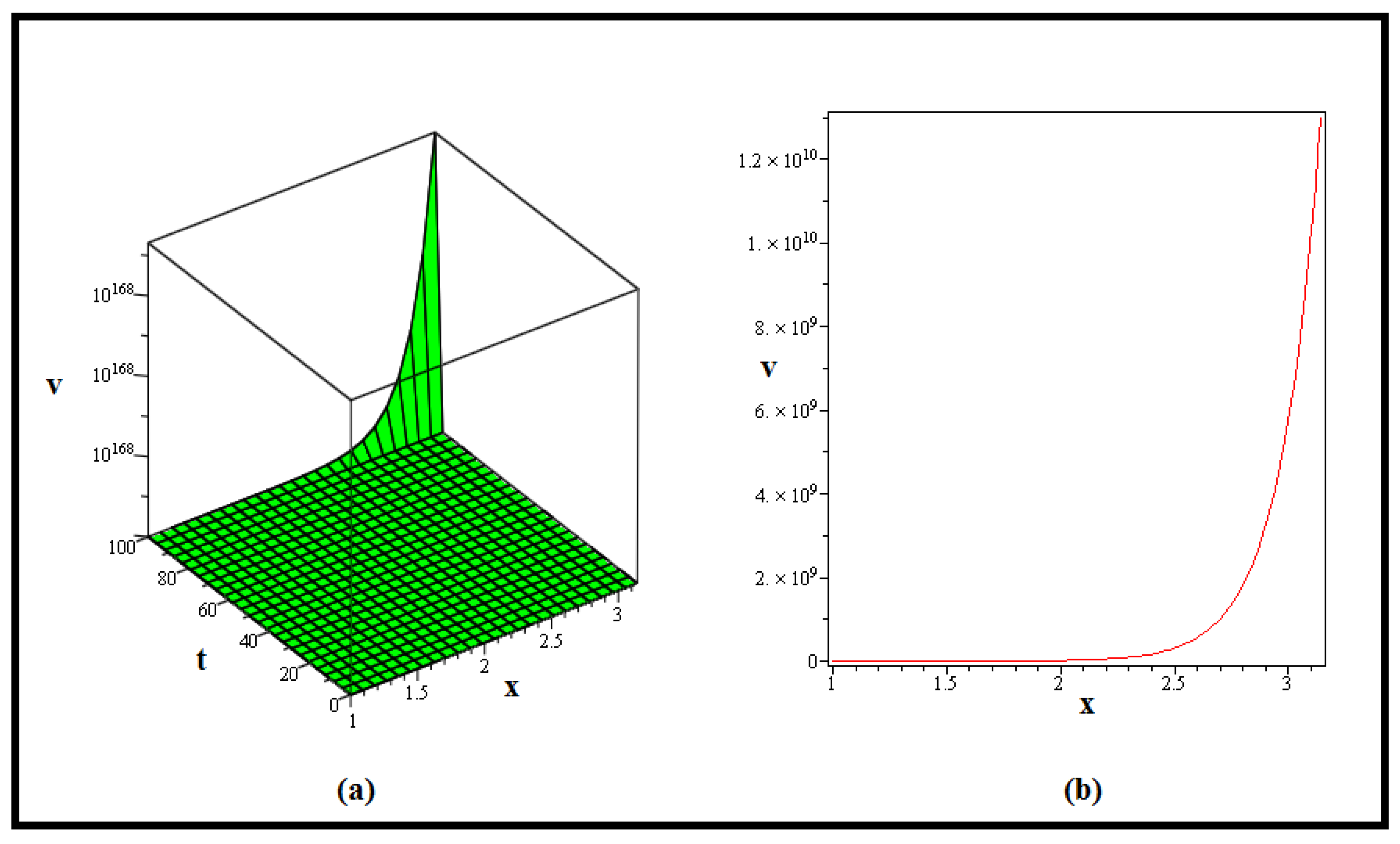
Remark 1. 

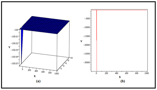
Figure 1 shows a singular kink wave. A single kink wave is a sort of localised disturbance distinguished by a quick and dramatic shift in the amplitude and phase of the wave. It involves a sharp transition between two states, which is much more obvious in the event of a solitary kink, resulting in a sudden and steep leap. A singular kink wave could represent an intense and highly localised disturbance in the pressure field in the context of a model such as the FKSE describing pressure waves in liquid–gas bubbly mixtures, potentially caused by specific conditions within the mixture that lead to a dramatic variation in the wave’s behaviour.

Remark 2. 

A multi-kinks profile is displayed in Figure 2. A multi-kink wave is a kink wave with numerous gentle transitions between distinct states inside a single waveform. During transmission, this phenomenon retains its shape and placements. Multi-kink waves display complicated, different transitions in the FKSE, which describes pressure waves in liquid–gas bubble mixes, exhibiting intricate pressure dynamics caused by various densities and characteristics within the mixture. These patterns are formed by the interaction of nonlinear and dispersive effects in the FKSE, which improves our understanding of wave behaviours in such systems.

Remark 3. 

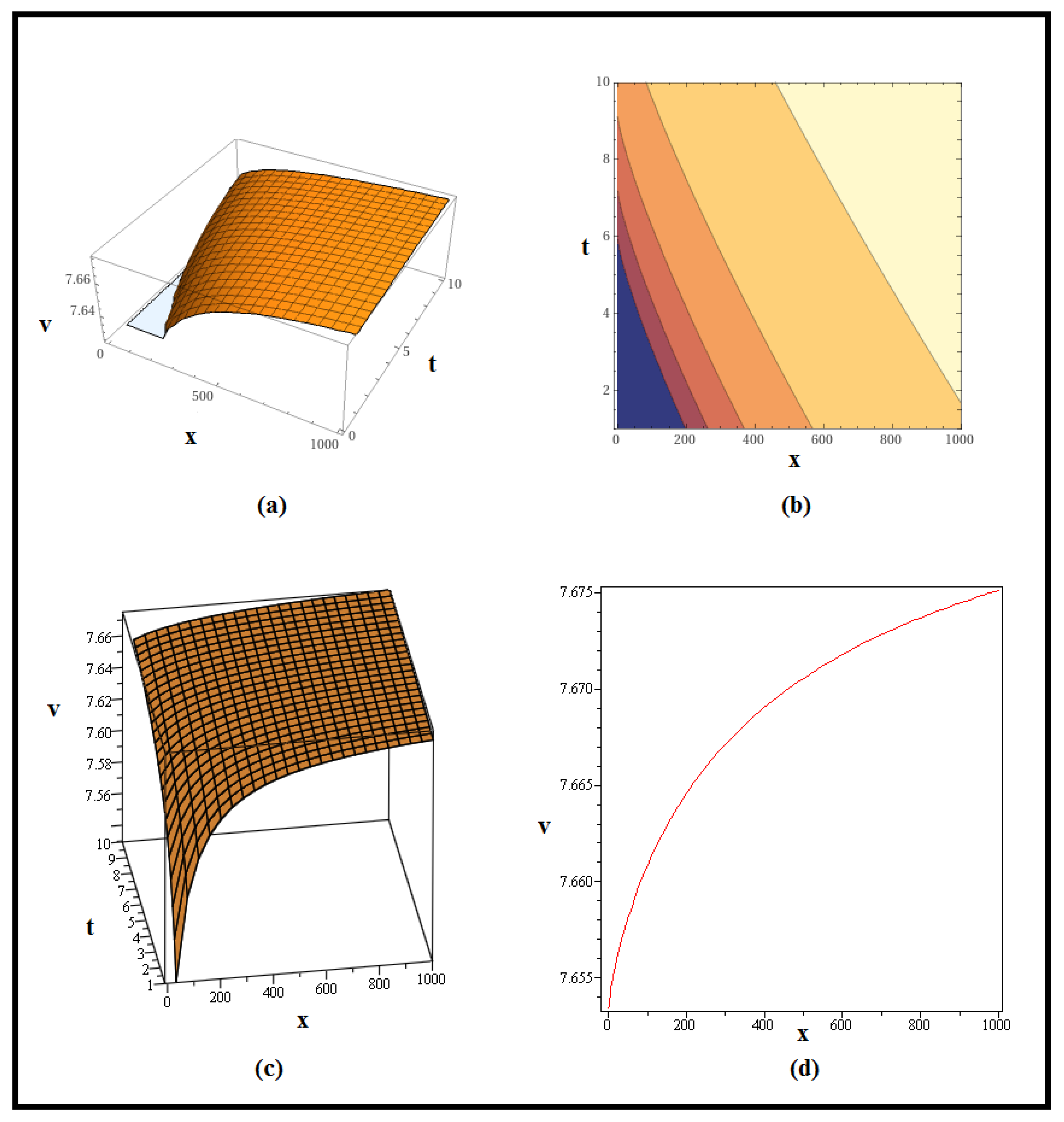
Figure 3 shows a shock wave profile. A shock wave is a sudden and powerful disturbance in a medium, characterised by an abrupt increase in pressure, density, and temperature as the wave passes through. In the context of the previously stated model, such as the FKSE describing pressure waves in liquid–gas bubble mixes, a shock wave might result from a quick change in circumstances inside the mixture, creating an abrupt shift in pressure and density. The interaction of nonlinearity and dispersion in the model might result in the development of shock waves as these waves travel through the bubbly liquid, impacting pressure dynamics and perhaps triggering dynamic changes within the medium.

Remark 4. 

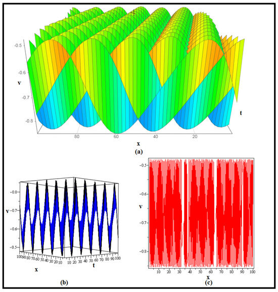
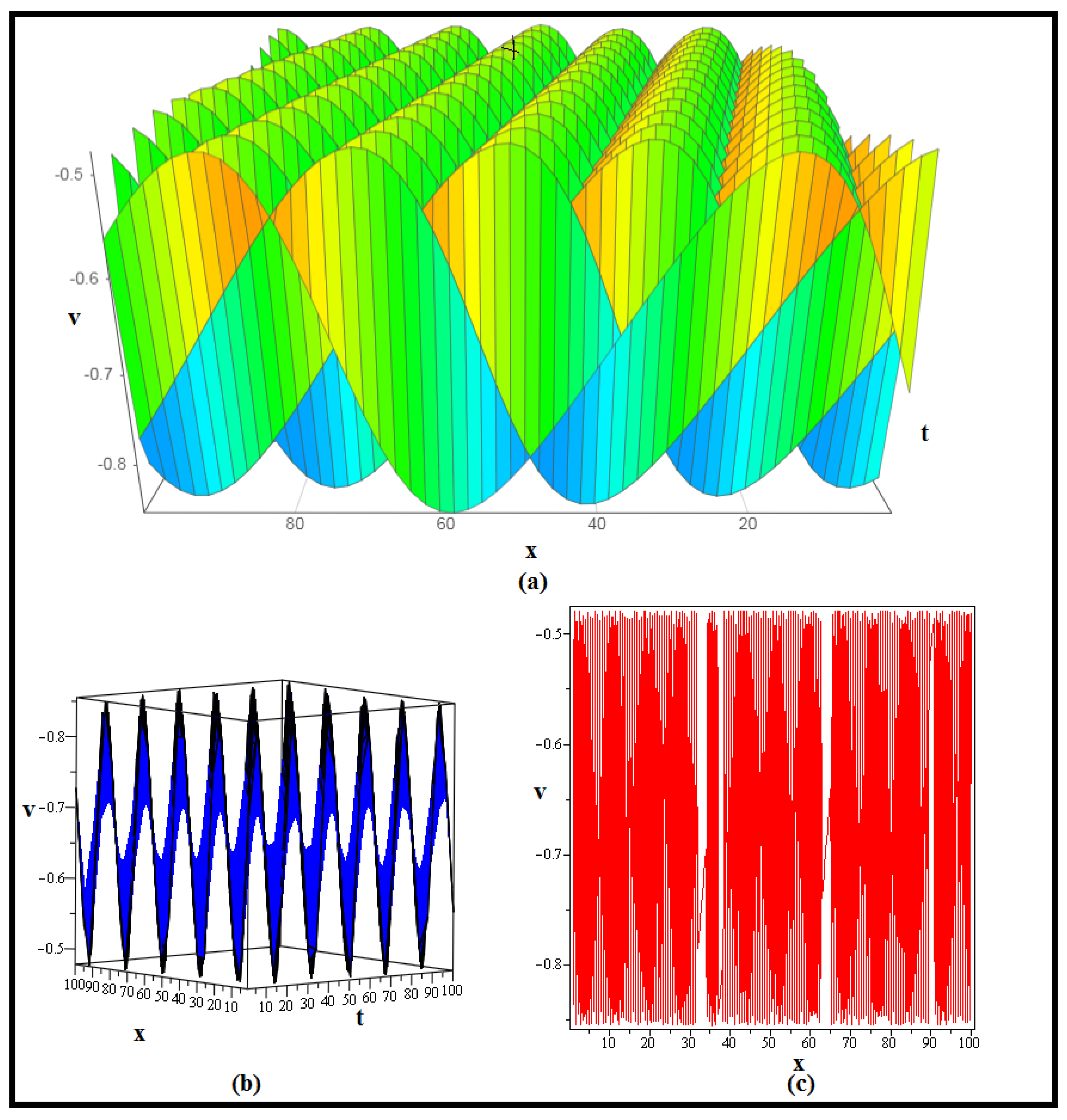
Figure 4 depicts a periodic wave profile. A periodic wave is a repeating oscillation with a constant pattern across time and regular crests and troughs. A periodic wave would indicate a recurring fluctuation in pressure and density inside the mixture as the wave propagates in the context of the earlier stated model, such as the FKSE explaining pressure waves in liquid–gas bubble mixes. The model’s nonlinearity and dispersion effects may cause periodic waves with specified frequencies and wavelengths to arise, representing the cyclic behaviour of pressure variations in the bubbly liquid medium.

Remark 5. 

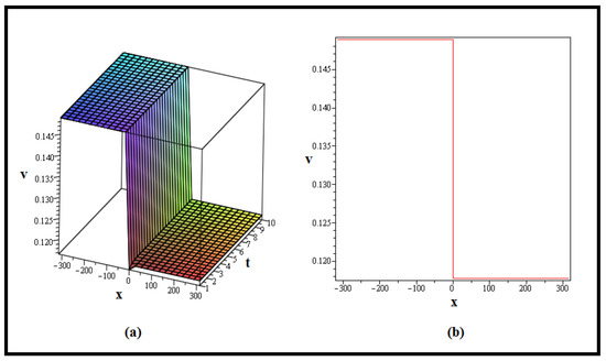
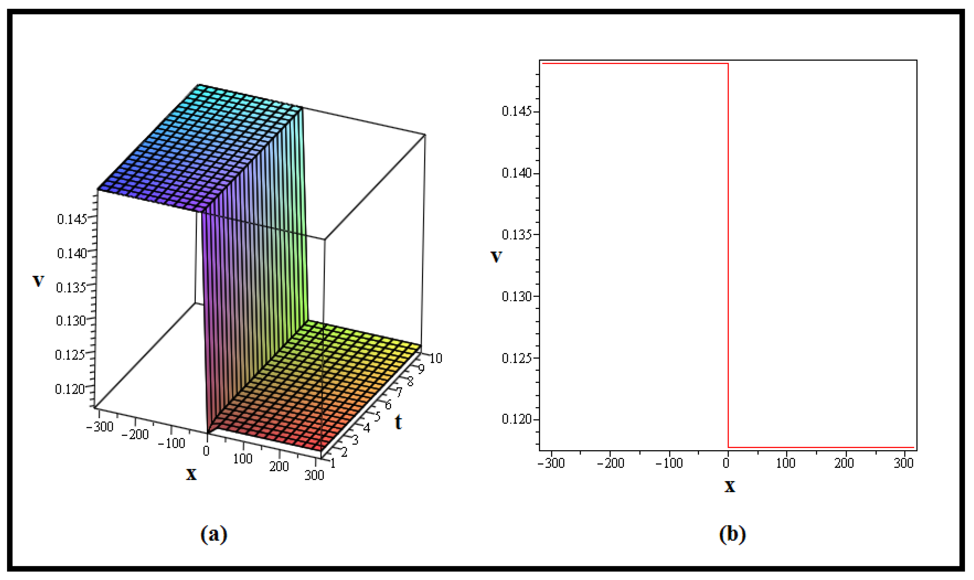
Figure 5 shows a kink wave profile. A kink wave is a form of soliton, or solitary wave that keeps its shape and velocity during propagation due to a balance of dispersion and nonlinearity. A kink wave relates to a localised disturbance or wavefront that demonstrates an abrupt transition between two distinct states in the context of the previously stated model, such as the FKSE describing pressure waves in liquid–gas bubble mixes. Kink waves are an important characteristic in many physical systems, including fluid dynamics, plasma physics, and others, since they occur smoothly across a finite distance. Kink waves can help us to understand the behaviour of pressure waves in bubbly liquids, where nonlinear and dispersive processes shape the dynamics of these waves.

Remark 6. 

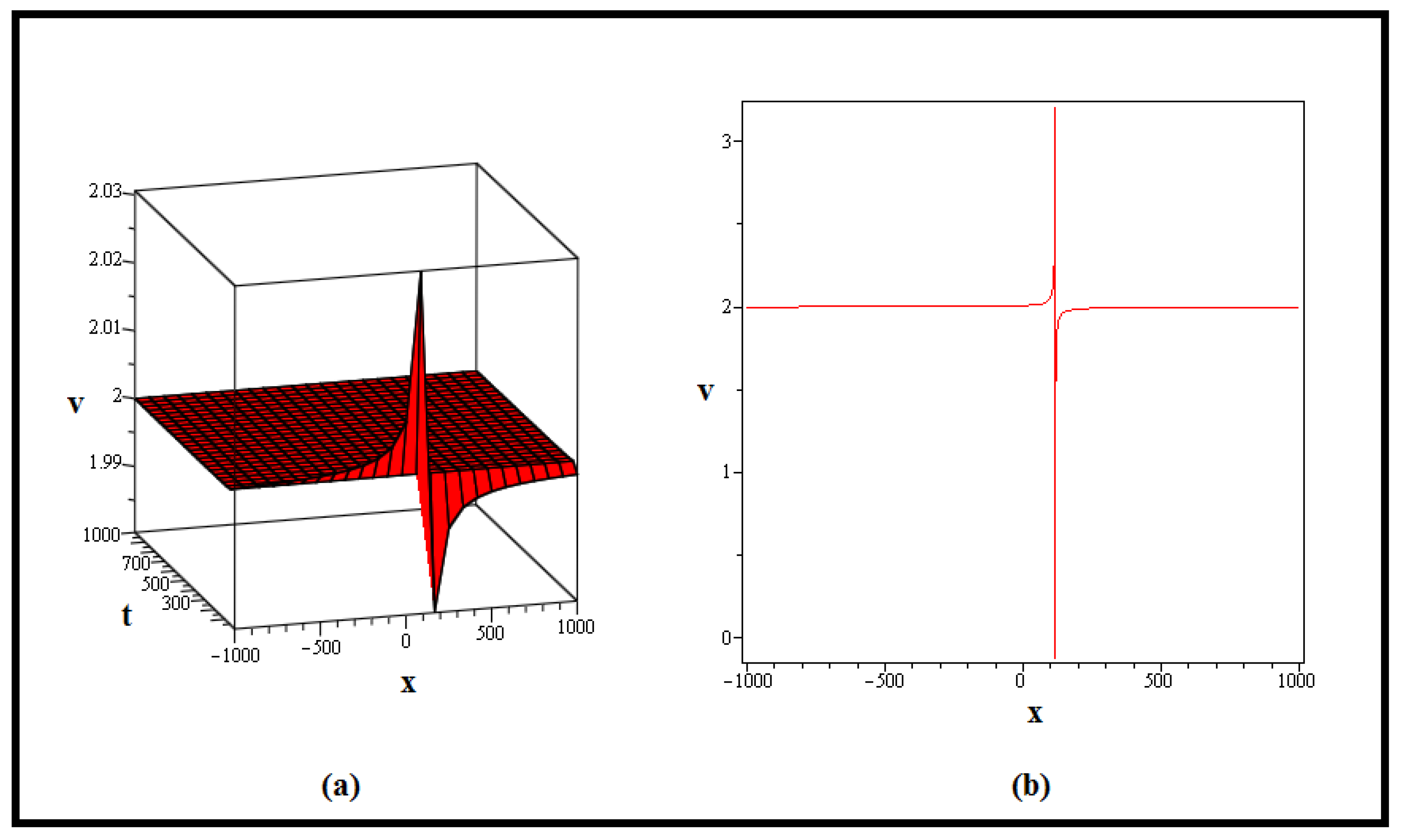
Figure 6 shows a lump wave. A lump wave, also known as a lumpy wave or a compacton, is a form of a solitary wave characterised by a localised peak or lump that travels with minimum dispersion while preserving its structure. A lump wave, in the context of the previously discussed model, such as the FKSE describing pressure waves in liquid–gas bubbly mixtures, could represent a concentrated region of pressure variation within the mixture that retains its distinctive shape over distance due to the balance between nonlinearity and dispersion. Lump waves are fascinating phenomena because they display both wave-like and particle-like behaviour. Their presence in complicated systems such as bubbly liquids might provide information on the intricate pressure dynamics inside the mixture.

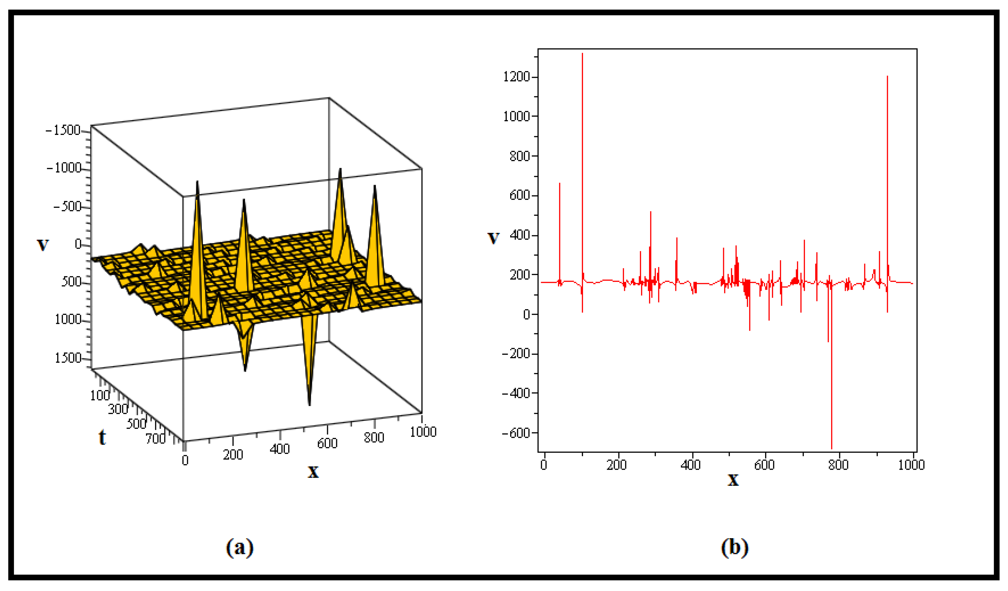
Remark 7. 

Figure 7 also shows another shock wave. A shock wave is a fast and intense disturbance in a medium that causes a sudden rise in pressure, density, and temperature as it passes through. A shock wave might emerge from a quick change in circumstances inside the mixture, creating an abrupt shift in pressure and density in the context of the earlier stated model, such as the FKSE explaining pressure waves in liquid–gas bubbly mixes. The model’s interaction of nonlinearity and dispersion may result in the development of shock waves, as these waves travel through the bubbly liquid, impacting pressure dynamics and perhaps triggering dynamic changes within the medium.

5. Conclusions

We have investigated the intricacies of soliton dynamics within the context of the FKSE, which governs pressure waves in liquid–gas bubbly mixes. Furthermore, we have discovered a diverse range of soliton solutions using the mEDAM approach, including kink, solitary kink, multi-kink, lump, and periodic wave patterns. Our investigation highlighted the interaction of nonlinearity and dispersion, demonstrating their contributions to the various behaviours of waves in complex fluid systems. These answers have far-reaching ramifications that go beyond mathematical physics, influencing domains such as optical fibres, plasma physics, and other practical sciences. We proved the practical importance of these solutions by graphical depiction and thorough analysis, emphasising their role in improving our understanding of wave events across several disciplines. This research increases our understanding of soliton dynamics by delving further into the various complexities of wave propagation through complicated media. Further research has the potential to yield innovative insights and practical applications, promoting advances in both theoretical knowledge and real-world implementations. Moreover, the adaptability of the mEDAM technique we offer is demonstrated by its ability to handle extremely nonlinear systems. In contrast to the approaches outlined in the literature review, our system speeds the translation of a model into a nonlinear algebraic equation system. This fast procedure allows for the development of many families of soliton solutions, distinguishing it from other methods that primarily allow for a more thorough study of the model. It should be noted, however, that this strategy may find difficulties in scenarios involving very complicated models or circumstances in which the homogenous balancing principle is not applicable.

References

- Kaplan, M.; Bekir, A. The modified simple equation method for solving some fractional-order nonlinear equations. Pramana 2016, 87, 1–5. [Google Scholar] [CrossRef]
- Zhang, S.; Zhang, H.Q. Fractional sub-equation method and its applications to nonlinear fractional PDEs. Phys. Lett. A 2011, 375, 1069–1073. [Google Scholar] [CrossRef]
- Kumar, D.; Singh, J.; Baleanu, D. Numerical computation of a fractional model of differential-difference equation. J. Comput. Nonlinear Dyn. 2016, 11, 061004. [Google Scholar] [CrossRef]
- Gurefe, Y. The generalized Kudryashov method for the nonlinear fractional partial differential equations with the beta-derivative. Rev. Mex. Física 2020, 66, 771–781. [Google Scholar] [CrossRef]
- Khan, H.; Shah, R.; Gómez-Aguilar, J.F.; Baleanu, D.; Kumam, P. Travelling waves solution for fractional-order biological population model. Math. Model. Nat. Phenom. 2021, 16, 32. [Google Scholar] [CrossRef]
- Zayed, E.M.; Amer, Y.A.; Shohib, R.M. The fractional complex transformation for nonlinear fractional partial differential equations in the mathematical physics. J. Assoc. Arab Univ. Basic Appl. Sci. 2016, 19, 59–69. [Google Scholar] [CrossRef]
- Neirameh, A. New fractional calculus and application to the fractional-order of extended biological population model. Bol. Soc. Parana. Mate. 2018, 36, 115–128. [Google Scholar] [CrossRef]
- Tarasov, V.E. On history of mathematical economics: Application of fractional calculus. Mathematics 2019, 7, 509. [Google Scholar] [CrossRef]
- Karamali, G.; Dehghan, M.; Abbaszadeh, M. Numerical solution of a time-fractional PDE in the electroanalytical chemistry by a local meshless method. Eng. Comput. 2019, 35, 87–100. [Google Scholar] [CrossRef]
- Mendez, A.J. On the propagation of regularity for solutions of the fractional Korteweg-de Vries equation. J. Differ. Equ. 2020, 269, 9051–9089. [Google Scholar] [CrossRef]
- Veeresha, P.; Prakasha, D.G.; Baskonus, H.M. Novel simulations to the time-fractional Fisher’s equation. Math. Sci. 2019, 13, 33–42. [Google Scholar] [CrossRef]
- Kurt, A.; Çenesiz, Y.; Tasbozan, O. On the solution of Burgers’ equation with the new fractional derivative. Open Phys. 2015, 13, 355–360. [Google Scholar] [CrossRef]
- Saha Ray, S.; Das, N. New optical soliton solutions of fractional perturbed nonlinear Schrödinger equation in nanofibers. Mod. Phys. Lett. B 2022, 36, 2150544. [Google Scholar] [CrossRef]
- Mirzazadeh, M. Topological and non-topological soliton solutions to some time-fractional differential equations. Pramana 2015, 85, 17–29. [Google Scholar] [CrossRef]
- Saha Ray, S.; Sagar, B. Numerical soliton solutions of fractional modified (2 + 1)-dimensional Konopelchenko–Dubrovsky equations in plasma physics. J. Comput. Nonlinear Dyn. 2022, 17, 011007. [Google Scholar] [CrossRef]
- Bouzari Liavoli, F.; Fakharian, A.; Khaloozadeh, H. Sub-optimal controller design for time-delay nonlinear partial differential equation systems: An extended state-dependent differential Riccati equation approach. Int. J. Syst. Sci. 2023, 54, 1815–1840. [Google Scholar] [CrossRef]
- Razzaq, W.; Zafar, A.; Ahmed, H.M.; Rabie, W.B. Construction solitons for fractional nonlinear Schrödinger equation with β-time derivative by the new sub-equation method. J. Ocean Eng. Sci. 2022, 17, 1–7. [Google Scholar] [CrossRef]
- Khan 2022, H.; Baleanu, D.; Kumam, P.; Al-Zaidy, J.F. Families of travelling waves solutions for fractional-order extended shallow water wave equations, using an innovative analytical method. IEEE Access 2019, 7, 107523–107532. [Google Scholar] [CrossRef]
- Alsharidi, A.K.; Bekir, A. Discovery of New Exact Wave Solutions to the M-Fractional Complex Three Coupled Maccari’s System by Sardar Sub-Equation Scheme. Symmetry 2023, 15, 1567. [Google Scholar] [CrossRef]
- Gaber, A.; Ahmad, H. Solitary wave solutions for space-time fractional coupled integrable dispersionless system via generalized kudryashov method. Facta Univ. Ser. Math. Inform. 2021, 35, 1439–1449. [Google Scholar] [CrossRef]
- Dubey, S.; Chakraverty, S. Application of modified extended tanh method in solving fractional order coupled wave equations. Math. Comput. Simul. 2022, 198, 509–520. [Google Scholar] [CrossRef]
- Muhamad, K.A.; Tanriverdi, T.; Mahmud, A.A.; Baskonus, H.M. Interaction characteristics of the Riemann wave propagation in the (2 + 1)-dimensional generalized breaking soliton system. Int. J. Comput. Math. 2023, 100, 1340–1355. [Google Scholar] [CrossRef]
- Rezazadeh, H.; Mirhosseini-Alizamini, S.M.; Neirameh, A.; Souleymanou, A.; Korkmaz, A.; Bekir, A. Fractional Sine–Gordon equation approach to the coupled higgs system defined in time-fractional form. Iran. J. Sci. Technol. Trans. A Sci. 2019, 43, 2965–2973. [Google Scholar] [CrossRef]
- Yasmin, H.; Aljahdaly, N.H.; Saeed, A.M.; Shah, R. Investigating Symmetric Soliton Solutions for the Fractional Coupled Konno–Onno System Using Improved Versions of a Novel Analytical Technique. Mathematics 2023, 11, 2686. [Google Scholar] [CrossRef]
- Yasmin, H.; Aljahdaly, N.H.; Saeed, A.M.; Shah, R. Investigating Families of Soliton Solutions for the Complex Structured Coupled Fractional Biswas–Arshed Model in Birefringent Fibers Using a Novel Analytical Technique. Fractal Fract. 2023, 7, 491. [Google Scholar] [CrossRef]
- Yasmin, H.; Aljahdaly, N.H.; Saeed, A.M. and Shah, R. Probing Families of Optical Soliton Solutions in Fractional Perturbed Radhakrishnan–Kundu–Lakshmanan Model with Improved Versions of Extended Direct Algebraic Method. Fractal Fract. 2023, 7, 512. [Google Scholar] [CrossRef]
- Seadawy, A.R.; Iqbal, M.; Lu, D. Nonlinear wave solutions of the Kudryashov–Sinelshchikov dynamical equation in mixtures liquid-gas bubbles under the consideration of heat transfer and viscosity. J. Taibah Univ. Sci. 2019, 13, 1060–1072. [Google Scholar] [CrossRef]
- Kudryashov, N.A.; Sinelshchikov, D.I. Nonlinear waves in bubbly liquids with consideration for viscosity and heat transfer. Phys. Lett. A 2010, 374, 2011–2016. [Google Scholar] [CrossRef]
- Yue, C.; Khater, M.; Attia, R.A.; Lu, D. The plethora of explicit solutions of the fractional KS equation through liquid–gas bubbles mix under the thermodynamic conditions via Atangana–Baleanu derivative operator. Adv. Differ. Equ. 2020, 2020, 62. [Google Scholar] [CrossRef]
- Korteweg, D.J.; De Vries, G. XLI. On the change of form of long waves advancing in a rectangular canal and on a new type of long stationary waves. Lond. Edinb. Dublin Philos. Mag. J. Sci. 1895, 39, 422–443. [Google Scholar] [CrossRef]
- Yang, X.J.; Tenreiro Machado, J.A.; Baleanu, D.; Cattani, C. On exact traveling-wave solutions for local fractional Korteweg-de Vries equation. Chaos Interdiscip. J. Nonlinear Sci. 2016, 26, 084312. [Google Scholar] [CrossRef] [PubMed]
- Shu, J.J. The proper analytical solution of the Korteweg-de Vries-Burgers equation. arXiv 2014, arXiv:1403.3636. [Google Scholar]
- Saad 2014, K.M.; AL-Shareef, E.H.; Alomari, A.K.; Baleanu, D.; Gómez-Aguilar, J.F. On exact solutions for time-fractional Korteweg-de Vries and Korteweg-de Vries-Burger’s equations using homotopy analysis transform method. Chin. J. Phys. 2020, 63, 149–162. [Google Scholar] [CrossRef]
- Ryabov, P.N.; Sinelshchikov, D.I.; Kochanov, M.B. Application of the Kudryashov method for finding exact solutions of the high order nonlinear evolution equations. Appl. Math. Comput. 2011, 218, 3965–3972. [Google Scholar] [CrossRef]
- Liu, J.G.; Yang, X.J.; Feng, Y.Y.; Geng, L.L. Symmetry analysis of the generalized space and time fractional Korteweg–de Vries equation. Int. J. Geom. Methods Mod. Phys. 2021, 18, 2150235. [Google Scholar] [CrossRef]
- Gupta, A.K.; Ray, S.S. On the solitary wave solution of fractional Kudryashov–Sinelshchikov equation describing nonlinear wave processes in a liquid containing gas bubbles. Appl. Math. Comput. 2017, 298, 1–12. [Google Scholar] [CrossRef]
- Ali, K.K.; Maneea, M. New approximation solution for time-fractional Kudryashov-Sinelshchikov equation using novel technique. Alex. Eng. J. 2023, 72, 559–572. [Google Scholar] [CrossRef]
- Akram, G.; Sadaf, M.; Anum, N. Solutions of time-fractional Kudryashov–Sinelshchikov equation arising in the pressure waves in the liquid with gas bubbles. Opt. Quantum Electron. 2017, 49, 373. [Google Scholar] [CrossRef]
- Prakash, P. On group analysis, conservation laws and exact solutions of time-fractional Kudryashov–Sinelshchikov equation. Comput. Appl. Math. 2021, 40, 162. [Google Scholar] [CrossRef]
- Sarikaya, M.Z.; Budak, H.; Usta, H. On generalized the conformable fractional calculus. TWMS J. Appl. Eng. Math. 2019, 9, 792–799. [Google Scholar]
Disclaimer/Publisher’s Note: The statements, opinions and data contained in all publications are solely those of the individual author(s) and contributor(s) and not of MDPI and/or the editor(s). MDPI and/or the editor(s) disclaim responsibility for any injury to people or property resulting from any ideas, methods, instructions or products referred to in the content. |
© 2023 by the authors. Licensee MDPI, Basel, Switzerland. This article is an open access article distributed under the terms and conditions of the Creative Commons Attribution (CC BY) license (https://creativecommons.org/licenses/by/4.0/).