Fixed-Time Fractional-Order Sliding Mode Control for UAVs under External Disturbances

Abstract

The present paper investigates a fixed-time tracking control with fractional-order dynamics for a quadrotor subjected to external disturbances. After giving the formulation problem of a quadrotor system with six subsystems like a second-order system, a fractional-order sliding manifold is then designed to achieve a fixed-time convergence of the state variables. In order to cope with the upper bound of the disturbances, a switching fixed-time controller is added to the equivalent control law. Based on the switching law, fixed-time stability is ensured. All analysis and stability are proved using the Lyapunov approach. Finally, the higher performance of the proposed controller fixed-time fractional-order sliding mode control (FTFOSMC) is successfully compared to the two existing techniques through numerical simulations.

1. Introduction

1.1. Background and Motivation

In recent years, due to the fast convergence and high precision performance of finite/fixed-time stability, an increasing variety of control approaches have been developed [1]. In [2], the authors introduced a composite-learning-based finite-time controller that makes use of a disturbance observer. The fixed-time stability (FxTS) is an extension of the finite-time stability (FnTS) property. The settling period is uniformly constrained and independent of the initial conditions on the fixed-time stability [3]. Then, an adjustable control parameter for the settling time is explicitly added for more flexibility of nonlinear system control such as the control of unmanned aerial vehicles (UAV). The quadrotor system is considered a complex nonlinear system in terms of parametric uncertainties and disturbances [4]. To increase the performance of quadrotor control, fractional-order calculus is used in many works [5,6,7] to ensure the objectives of the fixed-time controller and compensate for unknown continuous disturbances.

Fractional calculus has been viewed for a long time as a purely mathematical and theoretical study with few practical applications [4]. The use of fractional calculus in engineering and physical systems has, however, received a lot of attention recently. The fractional-order sliding mode control is among the most impressive applications. Moreover, a variety of useful systems have been discovered, including quadrotor systems [5,6].

1.2. Related Works

During the last two decades, the field of engineering study has become increasingly interested in UAVs. In particular, due to their control and mechanical design, quadrotors are the most studied and utilized type of UAV [8]. Therefore, a number of controllers of various types have been developed, and fixed-time fractional-order sliding mode control was introduced by [6,9] to enhance the tracking effectiveness for nonlinear power systems and mobile robot systems, adaptive sliding mode control for fractional-order systems [10], adaptive parallel fractional sliding mode control [11], and fractional-order adaptive backstepping control in [12]. The researchers of [13] suggested the self-triggered sliding mode control for a quadrotor with disturbances. The literature has suggested a number of techniques to deal with this chattering problem, such as the high-order sliding mode control [14,15,16]. The sliding mode controller is one of the most dependable architectures for assuring the desired performance. The complicated version, such as the adaptive sliding mode controller, is more resilient to outside disturbances even if it is based on the law of integer-order law. Due to its offered performances, including high accuracy and insensitivity to disturbances, the most recent version of the fractional-order fixed-time controller is regarded as one of the best control techniques for the quadrotor system control [4]. In [17], fractional-order chaotic systems can be controlled and synchronized using a fractional-order fixed-time non-singular terminal sliding mode. Additionally, fractional order controllers can increase the stability of dynamical systems [18]. The finite-time stability ensures that the system’s trajectories converge to the desired target after some finite time is called the settling time or the convergence time. In addition to the advantages of finite time stability, fixed time stability involves finite time stable systems for which the minimum bound of the settling-time function is guaranteed to be independent of the initial conditions of the system and can a priori be adjusted [19]. In order to regulate controllable nonlinear systems with matching disturbances, fixed-time sliding mode controllers were devised [20,21]. The quadrotor system can converge to a stable range within an upper-bound convergence time thanks to the fixed-time stability, regardless of the initial operational states [22,23]. Therefore, distributed fixed-time control methods have been proposed in [24] to produce improved performances for the power system, whereas the fixed-time control approach can better overcome these drawbacks. However, the nonlinear system’s convergence time under the fixed-time control approach cannot be estimated directly and must be calculated by a sophisticated estimation function that is based on tuning parameters [25]. The control of fractional-order systems using a fixed time controller was proposed in [26]. Following the research presented above, an appropriate SMC can be built to more effectively establish fractional-order fixed-time control.

1.3. Contributions

Based on the above literature review and inspired from the fixed-time stability using fractional dynamics on the control design, this work instigates on the tracking control of UAVs subjected to disturbances. The use of the fractional order (FO) on the sliding mode variable with fixed-time convergences increases the faster performance of the system. Also, the switching controller developed in our work with FO and FxT property copes with perturbations. In the following part, we present the contributions of the paper.

• The suggested FTFOSMC can achieve the benefits of the SMC with a quick response and robustness. In addition, fractional calculus can provide the proposed control with more flexibility in parameter adjustment and perform an improved task of removing the chattering problem associated with the standard SMC.
• The proposed control approach has been applied to quadrotor systems and compared to the two existing techniques.
• With the suggested FTFOSMC, the Lyapunov function is used to analyze the fixed-time stability of the quadrotor system. Simulations are also used to confirm the effectiveness of the proposed control for the quadrotor system.

1.4. Outline

The rest of the paper is organized as follows. Section 2 presents some fundamental characteristics, definitions, and lemmas on fixed-time stability and fractional calculus. Section 3 presents the main results of this article. Section 4 provides simulation data that attest to the usefulness of the suggested controller. Finally, Section 5 draws conclusions and suggests paths for more research.

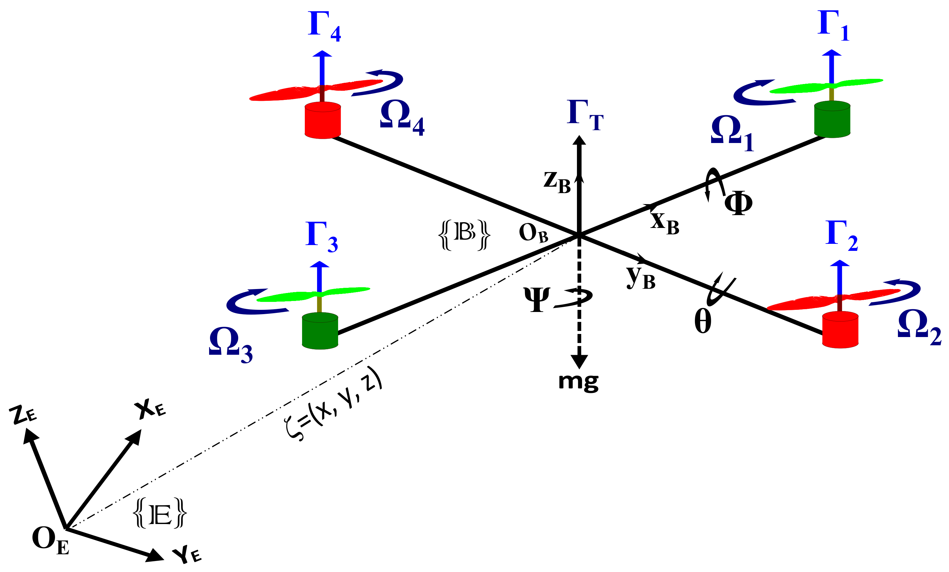
2. Problem Formulation and Preliminaries

2.1. Problem Definition and Formulation

The standard quadrotor system has two pairs of under-actuated propellers. In the body frame $O_b$, the position and attitude of the quadrotor UAV are specified as a rigid body model. The dynamic model of the quadrotor is developed using the quadrotor design in Figure 1. The orthogonal rotation matrix $R_T$, which can be parameterized by the roll, pitch, and yaw, is used to create this model, with Euler angles in the inertial frame of the earth E. The quadrotor UAV position is defined using x, y, and z in the $O_E$ frame.

Additionally, the quadrotor dynamic model in this research is created under the following assumptions. (i) The effect of the ground is neglected, (ii) the vehicle structure is symmetrical, (iii) both the blades and the vehicle frame are rigid, (iv) the disturbances should be bounded, (v) the torques and thrust generated by the rotor speeds are proportional to the square of the rotor rotating speeds. Many references use the Newton–Euler approach to obtain the dynamic model of the quadrotor [4,5,15].

$$\left\{\begin{array}{c}\ddot{\varphi }=j_1\dot{\theta }\dot{\psi }+j_2{\Omega }_r{\dot{\theta }}^2+j_3\dot{\varphi }+I_x^{-1}{\Gamma }_2+{\mathfrak{D}}_{\varphi }\hfill \\ \ddot{\theta }=j_4\dot{\varphi }\dot{\psi }+j_5{\Omega }_r{\dot{\varphi }}^2+j_6\dot{\theta }+I_y^{-1}{\Gamma }_3+{\mathfrak{D}}_{\theta }\hfill \\ \ddot{\psi }=j_7\dot{\varphi }\dot{\theta }+j_8\dot{\psi }+I_z^{-1}{\Gamma }_4+{\mathfrak{D}}_{\psi }\hfill \\ \ddot{x}=j_9\dot{x}+{\Gamma }_x+{\mathfrak{D}}_x\hfill \\ \ddot{y}=j_{10}\dot{y}+{\Gamma }_y+{\mathfrak{D}}_y\hfill \\ \ddot{z}=j_{11}\dot{z}+{\Gamma }_z+{\mathfrak{D}}_z.\hfill \end{array}\right.$$

(1)

With

$$j_1=(I_y-I_z)/I_x,j_2=-J_r/I_x,j_3=-K_{ax}/I_x,j_4=(I_z-I_x)/I_y$$

$$j_5=J_r/I_y,j_6=-K_{ay}/I_y,j_7=(I_x-I_y)/I_z,j_8=-K_{az}/I_z$$

$$j_9=-k_x/m,j_{10}=-k_y/m,j_{11}=-k_z/m.$$

where m is the mass of the body. The gravitational acceleration is denoted by g. Inertia moments of the quadrotor around the x, y, and z axes are denoted by $I_x,I_y$ and $I_z$. ${\Omega }_r={\Omega }_3+{\Omega }_4-{\Omega }_1-{\Omega }_2$ denotes the angular rotor speed. The torques and thrusts are the terms ${\Gamma }_{1-4}$ and ${\mathfrak{D}}_{x-\psi }$ represent the disturbances.

To stabilize the vehicle and follow the reference trajectory ${[{\varphi }_d,{\theta }_d,{\psi }_d,X_d,Y_d,Z_d]}^T$ in a finite amount of time, the goal of this study is to create a robust controller that generates the thrust magnitude and torque. The quadrotor has four control inputs ${[{\Gamma }_1,{\Gamma }_2,{\Gamma }_3,{\Gamma }_4]}^T$ and six outputs ${[\varphi ,\theta ,\psi ,X,Y,Z]}^T$. To simplify the control system design procedure, we provide the following definition of virtual control signals, which are used to acquire the overall thrust and required angles:

$$\left\{\begin{array}{c}{\Gamma }_x=(cos\left(\varphi \right)sin\left(\theta \right)cos\left(\psi \right)+sin\left(\varphi \right)sin\left(\psi \right))\frac{{\Gamma }_1}{m}\hfill \\ {\Gamma }_y=(cos\left(\varphi \right)sin\left(\theta \right)sin\left(\psi \right)-sin\left(\varphi \right)cos\left(\theta \right))\frac{{\Gamma }_1}{m}\hfill \\ {\Gamma }_z=cos\left(\varphi \right)cos\left(\theta \right)\frac{{\Gamma }_1}{m}-g.\hfill \end{array}\right.$$

(2)

We can determine the thrust ${\Gamma }_1$ and the two attitude angles ${\varphi }_d$ and ${\theta }_d$ based on the position controls we have obtained:

$$\left\{\begin{array}{c}{\varphi }_d=atan(c\left({\theta }_d\right)({\Gamma }_{x}s\left({\psi }_d\right)-{\Gamma }_{y}c\left({\psi }_d\right))/({\Gamma }_z+g))\hfill \\ {\theta }_d=atan({\Gamma }_{x}cos\left({\psi }_d\right)+{\Gamma }_{y}sin\left({\psi }_d\right)/({\Gamma }_z+g))\hfill \\ {\Gamma }_1=m\sqrt{{\Gamma }_x^2+{\Gamma }_y^2+{({\Gamma }_z+g)}^2}.\hfill \end{array}\right.$$

(3)

2.2. Fixed-Time Stability

The following section revises the FxTS of integer-order systems. Take a look at the integer-order system.

$$\dot{x}=g_1(t,x),x\left(0\right)=x_0,x\in {\mathbb{R}}^n.$$

(4)

where $x\in {\mathbb{R}}^n$ denotes the system state. The function $g_1:{\mathbb{R}}_{+}\times {\mathbb{R}}^n\mapsto {\mathbb{R}}^n$ is nonlinear, and if the origin is believed to be an equilibrium, then $g_1(t,0)=0$. The initial condition is $x_0=x\left(0\right)$. The following definitions are of specific importance.

Definition 1

(Finite-time design [3,27]). If the origin of (4) is globally asymptotically stable and all solutions to the equation reach the equilibrium point at some point in finite time, $x\left(t\right)=0$$\forall t\ge T\left(x\right(0\left)\right)$, then the origin is globally finite-time stable, where $T:{\mathbb{R}}^n\to {\mathbb{R}}^{+}\cup 0$ is the settling-time function.

Definition 2

(Fixed-time design [3]). If the settling-time function is bounded and the origin of system (4) is finite-time stable, then the basis is fixed-time stable, i.e., $\exists T_{max}>0:T\left(x\left(0\right)\right)\le T_{max}$, $\forall x\left(0\right)\in {\mathbb{R}}^n$.

Lemma 1.

Suppose there exists a continuous positive definite function $L_f\left(x\right)$ and that it satisfies the following equation [7,28].

$${\dot{L}}_f\left(x\right)+\kappa L_f{\left(x\right)}^{\mu }\le 0$$

where κ and μ are positive constants $\kappa >0,0<\mu <1$, the nonlinear system $\dot{x}=f(x,t)$ is finite-time stable, and the convergence time is limited by

$$T\le \frac{1}{\kappa (1-\mu )}{L}_f^{1-\mu }\left(x_0\right)$$

Lemma 2.

If there is a continuous unbounded function $L_f\left(x\right):{\mathbb{R}}^n\mapsto {\mathbb{R}}_{+}\cup 0$ such that $L_f\left(x\right)=0$ any solution $x\left(t\right)$ of (4) satisfies the following inequality [3,9,28]:

$$L_f\left(x\right)\le -{\delta }_1{L}_f^{{\rho }_1}\left(x\right)-{\delta }_2{L}_f^{{\rho }_2}\left(x\right).$$

(5)

with ${\delta }_1,{\delta }_2>0,{\rho }_1>1,0<{\rho }_2<1$, since the origin of the system in (4) is fixed-time stable, the settling time $T_1$ is defined:

$$T_1\le T_{max}:=\frac{1}{{\delta }_1\left({\rho }_1-1\right)}+\frac{1}{{\delta }_2\left(1-{\rho }_2\right)}.$$

(6)

2.3. Fractional-Order Calculus

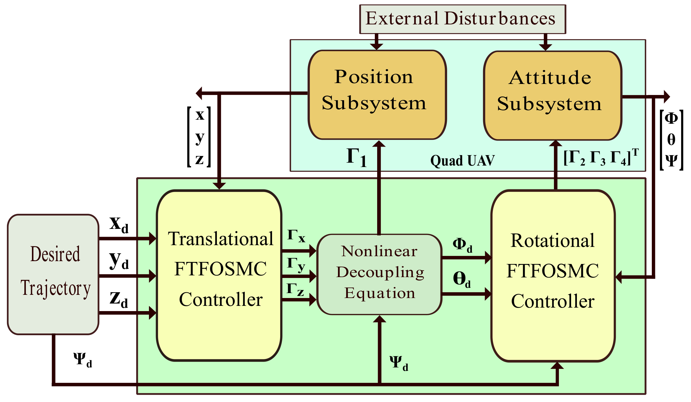
The most frequent fractional-order derivative of $\mathcal{G}\left(x\right)$ is the Caputo derivative written as [29]

$${}_{t_0}^C{D}_t^r\mathcal{G}\left(t\right)=\frac{1}{\Gamma (p-r)}{\int }_{t_0}^t\frac{{\mathcal{G}}^{\left(p\right)}\left(\tau \right)}{{(t-\tau )}^{r+1-p}}d\tau .$$

(7)

where r is the order of derivation, the Caputo derivative is indicated by the superscript C satisfying $p-1<r<p,p$ is an integer number and $\Gamma (.)$ is the Gamma function presented as

$$\Gamma \left(q\right)={\int }_0^{\infty }{e}^{-\nu }{\nu }^{q-1}d\nu ,q\in \mathbb{R}.$$

(8)

$\Gamma \left(q\right)$ denotes a general factorial expression for integer and non-integer values. As a result, $\Gamma \left(q\right)=q!$ when q is an integer value.

The expression for the function $\mathcal{G}$, the r th-order Caputo fractional integration is as follows [29]:

$$t_0{I}_t^r\mathcal{G}\left(t\right)={}_{t_0}{D}_t^{-r}\mathcal{G}\left(t\right)\frac{1}{\Gamma }\left(r\right){\int }_{t_0}^t\frac{\mathcal{G}\left(\tau \right)}{{(t-\tau )}^{1-r}}d\tau .$$

(9)

Properties:

• The following equality is satisfied by the Caputo derivative [29].

  $${}_{t_0}^C{D}_t^{r}f\left(t\right)\left({}_{t_0}^C{D}_t^{-\varrho }\mathcal{G}\left(t\right)\right)={}_{t_0}^C{D}_t^{r-\varrho }\mathcal{G}\left(t\right),r\ge \varrho \ge 0.$$

  (10)
• The following fractional-order expression can be used to represent the integer-order derivative [12].

  $$\dot{\mathcal{G}}\left(t\right)={}_0^C{D}_t^{1-r}\left({}_0^C{D}_t^r\mathcal{G}\left(t\right)\right).$$

  (11)

3. Control Design

In the following section, we present the fractional order fixed-time sliding mode for quadrotor tracking control with a quicker convergence. This is necessary for the design of the fractional order fixed-time sliding mode control scheme given in Figure 2.

3.1. External Disturbances

In general, the dynamics of the quadrotor can be summed up as follows:

$$\left\{\begin{array}{c}{\dot{y}}_k=y_{k+1}(k=1,3,5,7,9,11)\hfill \\ {\dot{y}}_{k+1}=g\left(y\right)+h\left(y\right){\Gamma }_i+{\mathfrak{D}}_i.\hfill \end{array}\right.$$

(12)

The quadrotor equations take into consideration external disturbances ${\mathfrak{D}}_{i=x,y,z,\varphi ,\theta ,\psi }$. The disturbances consider on the paper are

$$\begin{array}{c}\hfill \left\{\begin{array}{cc}{\mathfrak{D}}_{x,y,z}=\hfill & sin\left(t\right)\mathrm{m}/{\mathrm{s}}^{2}t<10\hfill \\ {\mathfrak{D}}_{x,y,z}=\hfill & 2sin\left(10t\right)\mathrm{m}/{\mathrm{s}}^{2}10<t<20\hfill \\ {\mathfrak{D}}_{x,y,z}=\hfill & 2sin\left(12t\right)\mathrm{m}/{\mathrm{s}}^{2}t>20.\hfill \end{array}\right.\end{array}$$

(13)

$$\begin{array}{c}\hfill \left\{\begin{array}{cc}{\mathfrak{D}}_{\varphi ,\theta ,\psi }=\hfill & sin\left(t\right)\mathrm{rad}/{\mathrm{s}}^{2}t<10\hfill \\ {\mathfrak{D}}_{\varphi ,\theta ,\psi }=\hfill & 2sin\left(10t\right)\mathrm{rad}/{\mathrm{s}}^{2}10<t<20\hfill \\ {\mathfrak{D}}_{\varphi ,\theta ,\psi }=\hfill & 2sin\left(12t\right)\mathrm{rad}/{\mathrm{s}}^{2}t>20.\hfill \end{array}\right.\end{array}$$

(14)

The quadrotor is employed on a tracking task in the presence of disturbances, and in order to improve robustness against disturbances, the desired trajectories $x_d,y_d,$ and $z_d$ are also square continuous. In the second scenario, the efficiency of the proposed control strategy, based on the FTFOSMC method for the path-following problem, has been tested under different disturbances using numerical simulations. In many applications, wind gust information can be obtained using unmanned aerial vehicles (UAVs) using wind sensors and an algorithm of estimation. This technique can be useful as feedback for robust control as well as a weightless substitute [30]. The estimated gust wind disturbance affecting the quadrotor is modeled as the input distributing the vehicle trajectory.

3.2. Fractional-Order Fixed Time Sliding Mode Control

In this section, a new FOFTSM controller for the attitude and position subsystems in the presence of disturbances will be presented. The state trajectory must be forced to track their reference values in a fixed time as the attitude system’s control goal. To accomplish this, the tracking errors can be represented as follows:

$$\begin{array}{cc}\hfill \left\{\begin{array}{c}{ϵ}_{\varphi }\left(t\right)=\varphi \left(t\right)-{\varphi }_d\left(t\right)\hfill \\ {ϵ}_{\theta }\left(t\right)=\theta \left(t\right)-{\theta }_d\left(t\right)\hfill \\ {ϵ}_{\psi }\left(t\right)=\psi \left(t\right)-{\psi }_d\left(t\right)\hfill \end{array}\right.,& \left\{\begin{array}{c}{ϵ}_x\left(t\right)=x\left(t\right)-x_d\left(t\right)\hfill \\ {ϵ}_y\left(t\right)=y\left(t\right)-y_d\left(t\right)\hfill \\ {ϵ}_z\left(t\right)=z\left(t\right)-z_d\left(t\right).\hfill \end{array}\right.\end{array}$$

(15)

To stabilize the altitude subsystem, the following fractional-order sliding manifold is suggested.

$$\begin{array}{cc}\hfill {\sigma }_z\left(t\right)& =I^{r_z}({\delta }_{z1}{\lfloor {ϵ}_z\left(t\right)\rceil }^{p_{z1}}+{\delta }_{z2}{\lfloor {ϵ}_z\left(t\right)\rceil }^{p_{z2}})+{\gamma }_z{D}^{1-r_z}{ϵ}_z\left(t\right)+D^{1-r_z}{\dot{ϵ}}_z\left(t\right).\hfill \end{array}$$

(16)

where ${\delta }_{z1},{\delta }_{z2}$ and ${\gamma }_z$ are positive constants, $p_{z1}>1$ and $0>p_{z2}>1$. The time-derivative order $r_z$ of ${\sigma }_z\left(t\right)$ is

$$\begin{array}{cc}\hfill D^{r_z}{\sigma }_z\left(t\right)& =({\delta }_{z1}{\lfloor {ϵ}_z\left(t\right)\rceil }^{p_{z1}}+{\delta }_{z2}{\lfloor {ϵ}_z\left(t\right)\rceil }^{p_{z2}})+{\gamma }_z{\dot{ϵ}}_z\left(t\right)+{\ddot{ϵ}}_z\left(t\right).\hfill \end{array}$$

(17)

$$\begin{array}{cc}\hfill D^{r_z}{\sigma }_z\left(t\right)& =({\delta }_{z1}{\lfloor {ϵ}_z\left(t\right)\rceil }^{p_{z1}}+{\delta }_{z2}{\lfloor {ϵ}_z\left(t\right)\rceil }^{p_{z2}})+{\gamma }_z{\dot{ϵ}}_z\left(t\right)+(j_{11}\dot{z}+{\Gamma }_z+{\mathfrak{D}}_z-{\ddot{z}}_d).\hfill \end{array}$$

(18)

3.3. Stability Analysis

Theorem 1.

The errors will converge to the origin in fixed time for the fractional-order sliding surface when the state errors satisfy the stability for the altitude subsystem, which is written as

$$T_{z1}\le T_{1max}:=\frac{{\gamma }_z}{{\delta }_{z1}(p_{z1}-1)}+\frac{{\gamma }_z}{{\delta }_{z2}(1-p_{z2})}.$$

(19)

Proof. 

Choosing the Lyapunov function as

$$L_{fz}=\left|{ϵ}_z\right|.$$

(20)

The time derivative of the Lyapunov function when $e_i\ne 0$ is as follows:

$${\dot{L}}_{fz}={\dot{ϵ}}_z·sign\left({ϵ}_z\right).$$

(21)

The equivalent ${\dot{ϵ}}_z=$$D^{1-r_z}\left(D^{r_z}{ϵ}_z\right)$, however according to properties, provides

$${\dot{L}}_{fz}=D^{r_z}\left(D^{1-r_z}{ϵ}_z\right)sign\left({ϵ}_z\right).$$

(22)

Replacing $D^{1-r_z}{ϵ}_z$ by Equation (16).

$$\begin{array}{cc}\hfill {\dot{L}}_{fz}& =-\frac{1}{{\gamma }_z}{D}^{r_z}sign\left({ϵ}_z\right)[I^{r_z}({\delta }_{z1}{\lfloor {ϵ}_z\left(t\right)\rceil }^{p_{z1}}+{\delta }_{z2}{\lfloor {ϵ}_z\left(t\right)\rceil }^{p_{z2}})+D^{1-r_z}{\dot{ϵ}}_z\left(t\right)-{\sigma }_z\left(t\right)].\hfill \end{array}$$

(23)

$$\begin{array}{c}\hfill {\dot{L}}_{fz}=-\frac{1}{{\gamma }_z}sign\left({ϵ}_z\right)[({\delta }_{z1}{\lfloor {ϵ}_z\left(t\right)\rceil }^{p_{z1}}+{\delta }_{z2}{\lfloor {ϵ}_z\left(t\right)\rceil }^{p_{z2}})+{\ddot{ϵ}}_z\left(t\right)].\end{array}$$

(24)

$$\begin{array}{cc}\hfill {\dot{L}}_{fz}& =-\frac{1}{{\gamma }_z}[({\delta }_{z1}sign{ϵ}_z\left(t\right){\lfloor {ϵ}_z\left(t\right)\rceil }^{p_{z1}}+{\delta }_{z2}sign{ϵ}_z\left(t\right){\lfloor {ϵ}_z\left(t\right)\rceil }^{p_{z2}})+|{\ddot{ϵ}}_z\left(t\right)\left|\right].\hfill \end{array}$$

(25)

As a result that ${\lfloor {ϵ}_z\left(t\right)\rceil }^{p_z}={\left|{ϵ}_z\left(t\right)\right|}^{p_z}sign\left({ϵ}_z\left(t\right)\right)$ and $sign\left({ϵ}_z\left(t\right)\right).sign\left({ϵ}_z\left(t\right)\right)=1$ it succeeds.

$$\begin{array}{cc}\hfill {\dot{L}}_{fz}& =-\frac{1}{{\gamma }_z}|{\ddot{ϵ}}_z\left(t\right)|-\frac{1}{{\gamma }_z}{\delta }_{z1}|{ϵ}_z{\left(t\right)|}^{p_{z1}}-\frac{1}{{\gamma }_z}{\delta }_{z2}|{ϵ}_z{\left(t\right)|}^{p_{z2}}<-\frac{1}{{\gamma }_z}{\delta }_{z1}|L_{fz}{|}^{p_{z1}}-\frac{1}{{\gamma }_z}{\delta }_{z2}|L_{fz}{)|}^{p_{z2}}.\hfill \end{array}$$

(26)

It is shown that the dynamic properties of a fractional order sliding manifold are demonstrated to converge to zero based on Lemma 2, and the settling time from (26) is

$$T_{z1}\le T_{zmax}:=\frac{{\gamma }_z}{{\delta }_{z1}\left(p_{z1}-1\right)}+\frac{{\gamma }_z}{{\delta }_{z2}\left(1-p_{z2}\right)}.$$

(27)

The outcome shows that Theorem 1 is properly proved for the fractional order sliding manifold that is being presented. By setting $D^{r_z}\sigma =0$. Assuming that, using (17) and (1) can be written as

$$\begin{array}{cc}\hfill & ({\delta }_{z1}{\lfloor {ϵ}_z\left(t\right)\rceil }^{p_{z1}}+{\delta }_{z2}{\lfloor {ϵ}_z\left(t\right)\rceil }^{p_{z2}})+{\gamma }_z{\dot{ϵ}}_z\left(t\right)+{\ddot{ϵ}}_z\left(t\right)=0\hfill \end{array}$$

(28)

Consequently, we obtained ${\ddot{ϵ}}_z\left(t\right)=\ddot{z}-{\ddot{z}}_d$.

$$\begin{array}{cc}\hfill & ({\delta }_{z1}{\lfloor {ϵ}_z\left(t\right)\rceil }^{p_{z1}}+{\delta }_{z2}{\lfloor {ϵ}_z\left(t\right)\rceil }^{p_{z2}})+{\gamma }_z{\dot{ϵ}}_z\left(t\right)+(\ddot{z}-{\ddot{z}}_d)=0\hfill \end{array}$$

(29)

From Equation (29), we have

$$\begin{array}{cc}\hfill & ({\delta }_{z1}{\lfloor {ϵ}_z\left(t\right)\rceil }^{p_{z1}}+{\delta }_{z2}{\lfloor {ϵ}_z\left(t\right)\rceil }^{p_{z2}})+{\gamma }_z{\dot{ϵ}}_z\left(t\right)+(j_{11}\dot{z}+{\Gamma }_z+{\mathfrak{D}}_z-{\ddot{z}}_d)=0\hfill \end{array}$$

(30)

As a result, we used Equation (31), and the equivalent control law ${\Gamma }_{zeq}$ is provided by

$$\begin{array}{cc}\hfill {\Gamma }_{zeq}& =-({\delta }_{z1}{\lfloor {ϵ}_z\left(t\right)\rceil }^{p_{z1}}+{\delta }_{z2}{\lfloor {ϵ}_z\left(t\right)\rceil }^{p_{z2}})-{\gamma }_z{\dot{ϵ}}_z\left(t\right)-j_{11}\dot{z}-{\mathfrak{D}}_z+{\ddot{z}}_d.\hfill \end{array}$$

(31)

The switching control law aims to reject the external elements and establish the robustness against their effects on the altitude subsystem.

$$\begin{array}{cc}\hfill {\Gamma }_{zsw}& =-D^{r-1}[{\delta }_{z3}{\lfloor {\sigma }_z\left(t\right)\rceil }^{p_{z3}}+{\delta }_{z4}{\lfloor {\sigma }_z\left(t\right)\rceil }^{p_{z4}}+{\lambda }_{3}sign\left(\sigma \right)].\hfill \end{array}$$

(32)

where ${\delta }_{z3},{\delta }_{z4}$, ${\lambda }_3$ are positive constants, $p_{z3}>1$ and $0>p_{z4}>1$ are positive constants, Furthermore, the virtual law for altitude control is given as

$$\begin{array}{cc}\hfill {\Gamma }_z& ={\Gamma }_{zeq}+{\Gamma }_{zsw}\hfill \\ & =-({\delta }_{z1}{\lfloor {ϵ}_z\left(t\right)\rceil }^{p_{z1}}+{\delta }_{z2}{\lfloor {ϵ}_z\left(t\right)\rceil }^{p_{z2}})-D^{r-1}[{\delta }_{z3}{\lfloor {\sigma }_z\left(t\right)\rceil }^{p_{z3}}\hfill \\ & +{\delta }_{z4}{\lfloor {\sigma }_z\left(t\right)\rceil }^{p_{z4}}+{\lambda }_{3}sign\left(\sigma \right)]-{\gamma }_z{\dot{ϵ}}_z\left(t\right)-j_{11}\dot{z}-{\mathfrak{D}}_z+{\ddot{z}}_d.\hfill \end{array}$$

(33)

□

Theorem 2.

Under the suggested control in Equation (33), the control error $e_z$ would reach the fractional order sliding manifold ${\sigma }_z=0$, and the upper bound of the convergence time at which this would occur is

$$T_{z2}\le T_{zmax}:=\frac{1}{{\delta }_{z3}(p_{z3}-1)}+\frac{1}{{\delta }_{z4}(1-p_{z4})}.$$

(34)

Proof. 

Using the Lyapunov function $L_{fz}=\left|{\sigma }_z\left(t\right)\right|$, the time derivative of this function can be obtained as

$${\dot{L}}_{fz}=sign\left({\sigma }_z\left(t\right)\right){\dot{\sigma }}_z\left(t\right).$$

(35)

Based on (1), (16) and (35), it can obtain the following equation:

$$\begin{array}{cc}\hfill {\dot{L}}_{fz}& =sign\left({\sigma }_z\left(t\right)\right)D^{1-r_z}{D}^r{\sigma }_z\left(t\right)\hfill \\ \hfill & =sign\left({\sigma }_z\left(t\right)\right)D^{1-r_z}(({\delta }_{z1}{\lfloor {ϵ}_z\left(t\right)\rceil }^{p_{z1}}+{\delta }_{z2}{\lfloor {ϵ}_z\left(t\right)\rceil }^{p_{z2}})+{\gamma }_z{\dot{ϵ}}_z\left(t\right)+{\ddot{ϵ}}_z\left(t\right))\hfill \\ \hfill =& sign\left({\sigma }_z\left(t\right)\right)D^{1-r_z}({\gamma }_z{\dot{ϵ}}_z+(j_{11}\dot{z}+{\Gamma }_z+{\mathfrak{D}}_z)-{\ddot{z}}_d+{\delta }_{z1}{\lfloor {ϵ}_z\left(t\right)\rceil }^{p_{z1}}+{\delta }_{z2}{\lfloor {ϵ}_z\left(t\right)\rceil }^{p_{z2}}).\hfill \end{array}$$

(36)

Based on Equation (33),

$$\begin{array}{cc}\hfill {\dot{L}}_{fz}& =sign\left({\sigma }_z\left(t\right)\right)D^{1-r_z}({\gamma }_z{\dot{ϵ}}_z\left(t\right)+(j_{11}\dot{z}+-({\delta }_{z1}{\lfloor {ϵ}_z\left(t\right)\rceil }^{p_{z1}}+{\delta }_{z2}{\lfloor {ϵ}_z\left(t\right)\rceil }^{p_{z2}})\hfill \\ & +D^{r-1}[{\delta }_{z3}{\lfloor {\sigma }_z\left(t\right)\rceil }^{p_{z3}}+{\delta }_{z4}{\lfloor {\sigma }_z\left(t\right)\rceil }^{p_{z4}}+{\lambda }_{3}sign\left(\sigma \right)]-{\gamma }_z{\dot{ϵ}}_z\left(t\right)-j_{11}\dot{z}\hfill \\ & -{\mathfrak{D}}_z+{\ddot{z}}_d+{\mathfrak{D}}_z)-{\ddot{z}}_d+{\delta }_{z1}{\lfloor {ϵ}_z\left(t\right)\rceil }^{p_{z1}}+{\delta }_{z2}{\lfloor {ϵ}_z\left(t\right)\rceil }^{p_{z2}})\hfill \\ \hfill & =-sign\left({\sigma }_z\left(t\right)\right)({\delta }_{z3}{\lfloor {\sigma }_z\left(t\right)\rceil }^{p_{z3}}+{\delta }_{z4}{\lfloor {\sigma }_z\left(t\right)\rceil }^{p_{z4}}).\hfill \end{array}$$

(37)

Consequently, we obtained $sign\left({\sigma }_z\left(t\right)\right).sign\left({\sigma }_z\left(t\right)\right)=1$.

$$\begin{array}{cc}\hfill {\dot{L}}_{fz}& =-sign\left({\sigma }_z\left(t\right)\right)({\delta }_{z3}{\lfloor {\sigma }_z\left(t\right)\rceil }^{p_{z3}}+{\delta }_{z4}{\lfloor {\sigma }_z\left(t\right)\rceil }^{p_{z4}})\hfill \\ \hfill & =-{\delta }_{z3}sign\left({\sigma }_z\right){\lfloor {\sigma }_z\rceil }^{p_{z3}}-{\delta }_{z4}sign\left({\sigma }_z\right){\lfloor {\sigma }_z\rceil }^{p_{z4}}\hfill \\ \hfill & =-{\delta }_{z3}|{\sigma }_z{|}^{p_{z3}}-{\delta }_{z4}{\left|{\sigma }_z\right|}^{p_{z4}}<0.\hfill \end{array}$$

(38)

From Lemma 2 in (5), the first part of Equation (38) is negative and ${\mathfrak{D}}_z$ denotes the upper bound of the disturbances satisfying $|{\mathfrak{D}}_z|$, thus V$\le 0$. The control error is effectively able to approach ${\sigma }_z$. Additionally, the convergence time at which the control error ${ϵ}_z$ is bounded by

$$T_{z2}\le T_{z2max}:=\frac{1}{{\delta }_{z3}(p_{z3}-1)}+\frac{1}{{\delta }_{z4}(1-p_{z4})}.$$

(39)

As a result, within an upper bound of time, the control error of the system would stabilize to zero. □

Corollary 1.

The closed-loop altitude subsystem (1), tracking error (15), terminal integral sliding mode surface (16), and controller (33) is fixed-time stable.

Proof. 

Based on Theorems 1 and 2, the estimate of the settling time can be demonstrated:

$$\begin{array}{c}\hfill T_z\le T_{z1}+T_{z2}.\end{array}$$

(40)

Then, from (27) and (39), we have

$$\begin{array}{cc}\hfill T_z\le & \frac{{\gamma }_z}{{\delta }_{z1}\left(p_{z1}-1\right)}+\frac{{\gamma }_z}{{\delta }_{z2}\left(1-p_{z2}\right)}+\frac{1}{{\delta }_{z3}(p_{z3}-1)}+\frac{1}{{\delta }_{z4}(1-p_{z4})}.\hfill \end{array}$$

(41)

It is demonstrated that the controller (33) can destroy the power quadrotor system in an upper bound of time using Theorems. However, there are many states and huge amounts of variables in the controller that cannot be measured directly in practice. In order to implement the controls, it is important to obtain the measurably variable. □

3.4. Proposed Control Laws for Quadrotor

The previous part developed the design of the proposed controller for the quadrotor system under external disturbances. The inner loop and outer-loop controls are presented in Figure 2 and aim to reduce the setting time and obtain higher accuracy and faster convergence. The control laws of the $\varphi$, $\theta$, $\psi$ subsystems are expressed by (42)–(44), respectively. The other control laws for the x, y, z subsystems are given by (45)–(47).

$$\begin{array}{cc}\hfill {\Gamma }_2& =-I_x[({\delta }_{\varphi 1}{\lfloor {ϵ}_{\varphi }\left(t\right)\rceil }^{p_{\varphi 1}}+{\delta }_{\varphi 2}{\lfloor {ϵ}_{\varphi }\left(t\right)\rceil }^{p_{\varphi 2}})-D^{r-1}[{\delta }_{\varphi 3}{\lfloor {\sigma }_{\varphi }\left(t\right)\rceil }^{p_{\varphi 3}}+{\delta }_{\varphi 4}{\lfloor {\sigma }_{\varphi }\left(t\right)\rceil }^{p_{\varphi 4}}\hfill \\ & +{\lambda }_{1}sign\left(\sigma \right)]+{\gamma }_{\varphi }{\dot{ϵ}}_{\varphi }\left(t\right)+j_3\dot{\varphi }+{\mathfrak{D}}_{\varphi }+j_1\dot{\theta }\dot{\psi }+j_2{\Omega }_r{\dot{\theta }}^2-{\ddot{\varphi }}_d].\hfill \end{array}$$

(42)

$$\begin{array}{cc}\hfill {\Gamma }_3& =-I_y[({\delta }_{\theta 1}{\lfloor {ϵ}_{\theta }\left(t\right)\rceil }^{p_{\theta 1}}+{\delta }_{\theta 2}{\lfloor {ϵ}_{\theta }\left(t\right)\rceil }^{p_{\theta 2}})-D^{r-1}[{\delta }_{\theta 3}{\lfloor {\sigma }_{\theta }\left(t\right)\rceil }^{p_{\theta 3}}+{\delta }_{\theta 4}{\lfloor {\sigma }_{\theta }\left(t\right)\rceil }^{p_{\theta 4}}\hfill \\ & +{\lambda }_{1}sign\left(\sigma \right)]+{\gamma }_{\theta }{\dot{ϵ}}_{\theta }\left(t\right)+j_6\dot{\theta }+{\mathfrak{D}}_{\theta }+j_4\dot{\varphi }\dot{\psi }+j_5{\Omega }_r{\dot{\varphi }}^2-{\ddot{\theta }}_d].\hfill \end{array}$$

(43)

$$\begin{array}{cc}\hfill {\Gamma }_4& =-I_z[({\delta }_{\psi 1}{\lfloor {ϵ}_{\psi }\left(t\right)\rceil }^{p_{\psi 1}}+{\delta }_{\psi 2}{\lfloor {ϵ}_{\psi }\left(t\right)\rceil }^{p_{\psi 2}})-D^{r-1}[{\delta }_{\psi 3}{\lfloor {\sigma }_{\psi }\left(t\right)\rceil }^{p_{\psi 3}}+{\delta }_{\psi 4}{\lfloor {\sigma }_{\psi }\left(t\right)\rceil }^{p_{\psi 4}}\hfill \\ & +{\lambda }_{1}sign\left(\sigma \right)]+{\gamma }_{\psi }{\dot{ϵ}}_{\psi }\left(t\right)+j_8\dot{\psi }+{\mathfrak{D}}_{\psi }+j_7\dot{\varphi }\dot{\theta }-{\ddot{\psi }}_d].\hfill \end{array}$$

(44)

$$\begin{array}{cc}\hfill {\Gamma }_x& =-({\delta }_{x1}{\lfloor {ϵ}_x\left(t\right)\rceil }^{p_{x1}}+{\delta }_{x2}{\lfloor {ϵ}_x\left(t\right)\rceil }^{p_{x2}})-D^{r-1}[{\delta }_{x3}{\lfloor {\sigma }_x\left(t\right)\rceil }^{p_{x3}}+{\delta }_{x4}{\lfloor {\sigma }_x\left(t\right)\rceil }^{p_{x4}}\hfill \\ & +{\lambda }_{1}sign\left(\sigma \right)]-{\gamma }_x{\dot{ϵ}}_x\left(t\right)-j_9\dot{x}-{\mathfrak{D}}_x+{\ddot{x}}_d.\hfill \end{array}$$

(45)

$$\begin{array}{cc}\hfill {\Gamma }_y& =-({\delta }_{y1}{\lfloor {ϵ}_y\left(t\right)\rceil }^{p_{y1}}+{\delta }_{y2}{\lfloor {ϵ}_y\left(t\right)\rceil }^{p_{y2}})-D^{r-1}[{\delta }_{y3}{\lfloor {\sigma }_y\left(t\right)\rceil }^{p_{y3}}\hfill \\ & +{\delta }_{y4}{\lfloor {\sigma }_y\left(t\right)\rceil }^{p_{y4}}+{\lambda }_{2}sign\left(\sigma \right)]-{\gamma }_y{\dot{ϵ}}_y\left(t\right)-j_{10}\dot{y}-{\mathfrak{D}}_y+{\ddot{y}}_d.\hfill \end{array}$$

(46)

$$\begin{array}{cc}\hfill {\Gamma }_z& =-({\delta }_{z1}{\lfloor {ϵ}_z\left(t\right)\rceil }^{p_{z1}}+{\delta }_{z2}{\lfloor {ϵ}_z\left(t\right)\rceil }^{p_{z2}})-D^{r-1}[{\delta }_{z3}{\lfloor {\sigma }_z\left(t\right)\rceil }^{p_{z3}}\hfill \\ & +{\delta }_{z4}{\lfloor {\sigma }_z\left(t\right)\rceil }^{p_{z4}}+{\lambda }_{3}sign\left(\sigma \right)]-{\gamma }_z{\dot{ϵ}}_z\left(t\right)-j_{11}\dot{z}-{\mathfrak{D}}_z+{\ddot{z}}_d.\hfill \end{array}$$

(47)

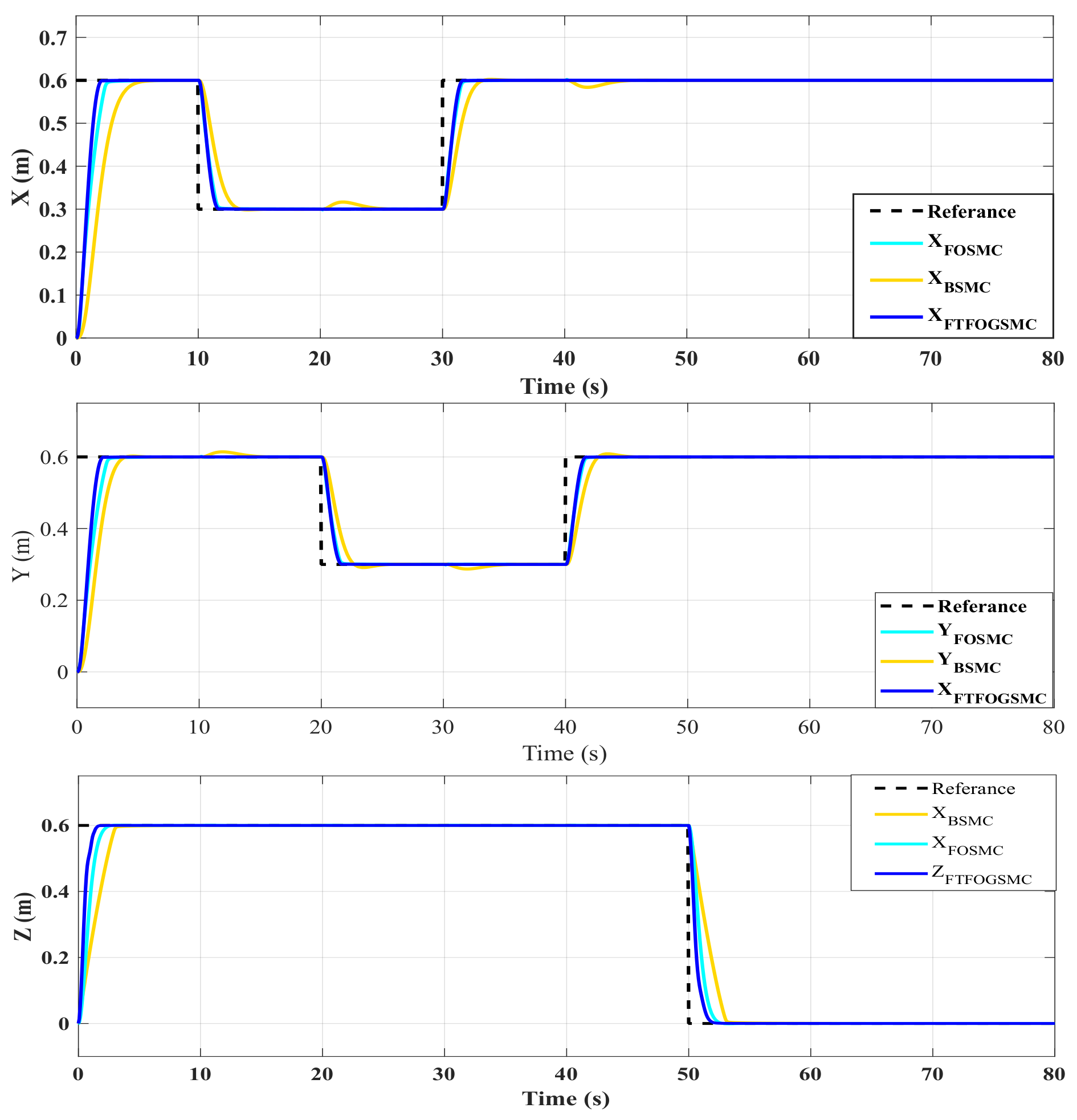
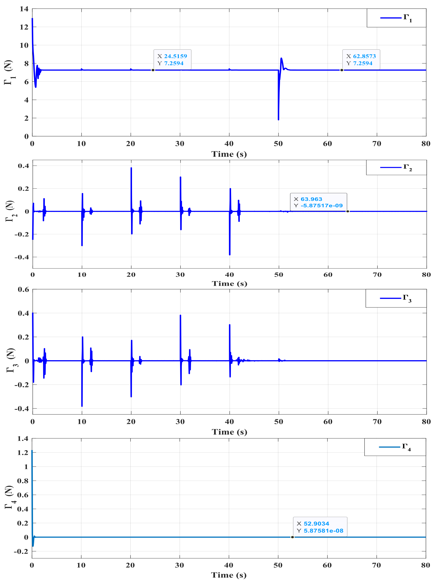
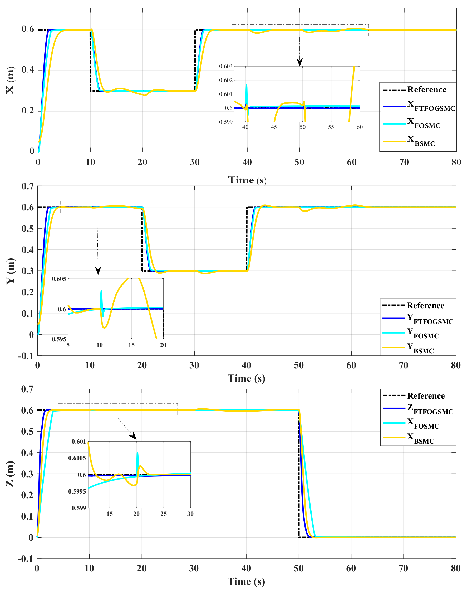
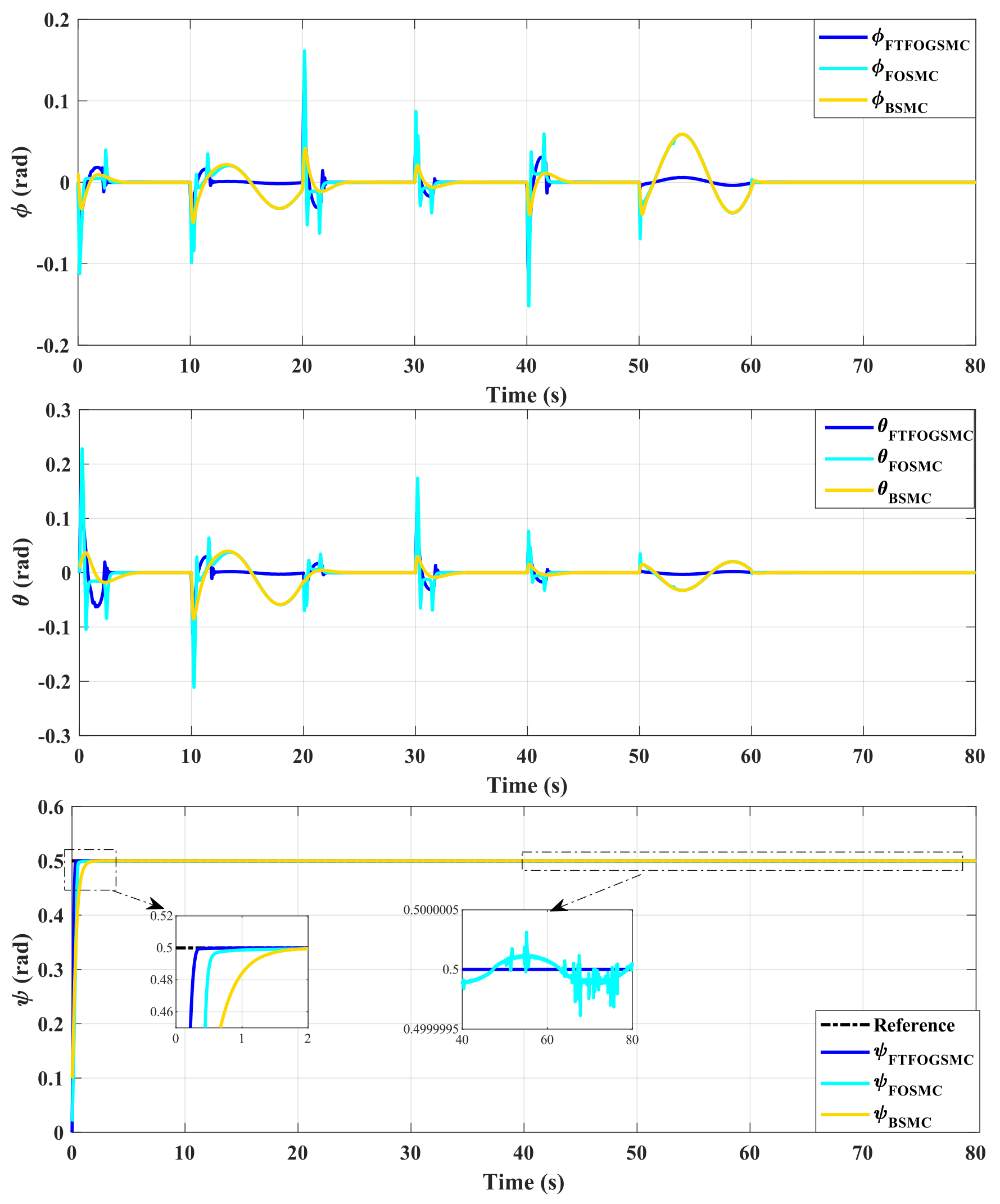
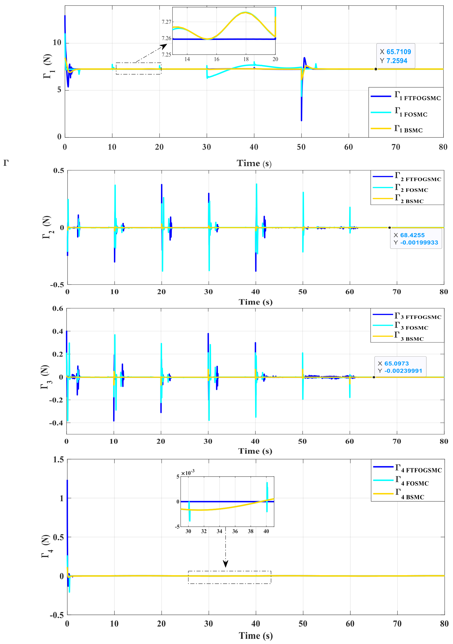
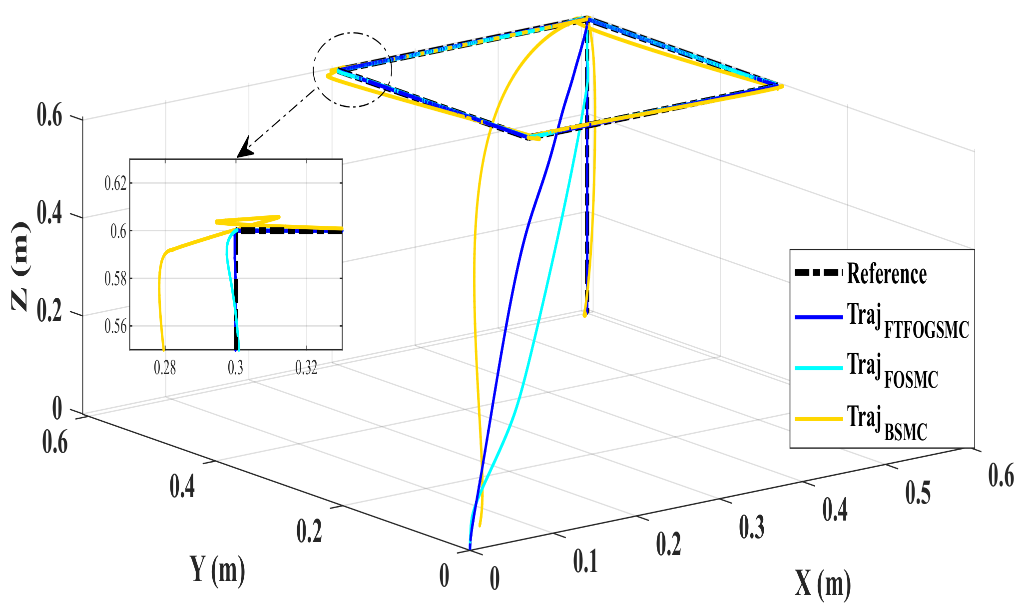
4. Simulation Results

In this section, simulations using the developed controllers are executed in MATLAB/Simulink software R2021a to demonstrate quadrotor trajectory tracking with/without disturbances and its robustness. A mathematical model of the quadrotor subsystems is developed based on the Newton–Euler formulation. The initial values of the quadrotor for the position and attitude subsystem are zeros.

Table 1. Quadrotor physical characteristics.

Symbol	Value	Unit
m	$0.74$	$\mathrm{kg}$
g	$9.81$	${\mathrm{s}}^{-2}·\mathrm{m}$
l	$0.5$	$\mathrm{m}$
$J_R$	$2.03\times {10}^{-5}$	$\mathrm{kg}·{\mathrm{m}}^2$
$I_x$	$2.24\times {10}^{-3}$	$\mathrm{kg}·{\mathrm{m}}^2$
$I_y$	$2.98\times {10}^{-3}$	$\mathrm{kg}·{\mathrm{m}}^2$
$I_z$	$4.80\times {10}^{-3}$	$\mathrm{kg}·{\mathrm{m}}^2$
$K_f$	$8.05\times {10}^{-6}$	$\mathrm{N}/{(\mathrm{rad}/\mathrm{s})}^2$
$K_m$	$2.42\times {10}^{-7}$	$\mathrm{N}·\mathrm{m}/{(\mathrm{rad}/\mathrm{s})}^2$

presents the physical parameters of the quadrotor.

Table 2. Parameters of the FTFOSM controller.

Symbol	Value	Symbol	Value	Symbol	Value
${\delta }_1$	$0.21$	$p_1$	$3.96$	$\gamma$	12
${\delta }_2$	$16.3$	$p_2$	$0.69$	$\lambda$	$0.82$
${\delta }_3$	$0.13$	$p_3$	$4.52$	$\kappa$	$0.68$
${\delta }_4$	$23.4$	$p_4$	$0.9$	ℵ	$0.34$

shows the parameters of the suggested control strategy.

In the present scenario, the quadrotor follows a square reference trajectory without disturbances, and the desired trajectory is specified by ${\psi }_d=0.5$ rad and Equations (48)–(50).

$$\begin{array}{c}\hfill x_d=\left\{\begin{array}{ccc}0.6\hfill & m\hfill & \mathrm{if}⩽10\mathrm{or}t>30.\hfill \\ 0.3\hfill & m\hfill & \mathrm{otherwise}.\hfill \end{array}\right.\end{array}$$

(48)

$$\begin{array}{c}\hfill y_d=\left\{\begin{array}{ccc}0.6\hfill & m\hfill & \mathrm{if}⩽20\mathrm{or}t>40.\hfill \\ 0.3\hfill & m\hfill & \mathrm{otherwise}.\hfill \end{array}\right.\end{array}$$

(49)

$$\begin{array}{c}\hfill z_d=\left\{\begin{array}{ccc}0.6\hfill & m\hfill & \mathrm{if}⩽50.\hfill \\ 0\hfill & m\hfill & \mathrm{otherwise}.\hfill \end{array}\right.\end{array}$$

(50)

The quadrotor in the second scenario follows travels along the reference trajectory, including disturbances in Equations (13) and (14).

Remark 1.

The fractional order operators allow for quick convergence of the state variables and improved quadrotor system responses. The recommended control approach offers more parameters for more precisely altering tracking performances from a practical standpoint.

Remark 2.

The compared simulation results are carried out using the two scenarios with and without disturbances, and the following starting circumstances: ${\left[x_0{y}_0{z}_0\right]}^T={\left[000\right]}^T$ and ${\left[{\varphi }_0{\theta }_0{\psi }_0\right]}^T={\left[000\right]}^T$.

Remark 3.

Many works demonstrated in the literature [31] successfully demonstrated the robustness of their algorithm through experiments without considering the influence of the ground effect and did not offer any proof of such scenarios. Therefore, the impact of the ground effect has often been neglected.

Figure 3 and Figure 4 demonstrate the attitude and position tracking of the quadrotor with and without disturbances, respectively, as desirable state variables are pushed to their target values in fixed-time, according to the simulation results.

Figure 3 displays the tracking performances of positions x, y, and z of the proposed and others compared the controllers’ step change of trajectory without disturbances. The proposed control method FTFOSMC gives a good tracking trajectory in terms of fast response and accuracy compared to that of FOSMC and BSMC.

The curves of Figure 4 are plotted to evaluate the tracking performances of the yaw, pitch, and roll angles using the three compared controllers. All these controllers allow the convergence of variables to desired values without taking into account the disturbances. However, the best convergence in finite time is ensured by the proposed controller. Therefore, the minimal pic magnitude and settling time is considered as the main advantages of the proposed technique compared to FOSMC and BSMC.

Figure 5 presents the performance of the control inputs of the quadrotor (${\Gamma }_T,{\Gamma }_2,{\Gamma }_3,{\Gamma }_4$) without disturbances. From these results, it can be observed that the control signals are smooth and converge to their original values. The pic of the signal is interpreted by the force needed to change the UAV position. The results prove the effectiveness of the proposed strategy. Despite the accuracy and the rapid convergence of the tracking, the UAV inputs reach the steady state faster without oscillations.

On the basis of the proposed FTFOSMC, a dual-loop practical fixed-time fractional order controller with disturbance rejection is developed. The position control performance with disturbances is shown in Figure 6. We can see that even when the references are changing quickly, the position controllers can accurately monitor the desired values.

Figure 7 shows the result of the suggested inner controller with disturbances, which enables the quadrotor to follow the reference angles.

Figure 8 shows the quadrotor control inputs under disturbance (${\Gamma }_1,{\Gamma }_2,{\Gamma }_3,{\Gamma }_4$). As can be seen from these figures, the control signals are smooth and converge to their initial values (7.26, 0, 0, 0) despite the presence of disturbance, which supports the efficacy of the FTFOSMC method.

Using the proposed controller, the 3D trajectory in Figure 9 with disturbances exhibits excellent tracking performance compared to that obtained using FOSMC and BSMC controllers.

Remark 4.

In order to help readers interested in developing experimental validation of the proposed control system, a test rig and a procedure for experimental validation of the results are described. To achieve this objective, the schematic diagram and list of components required to build the experimental drone test bench (see Figure 10) are detailed in this subsection [32]. This experimental test rig will be built to evaluate and confirm the proposed scenarios. Figure 10 illustrates the hardware design of the experimental platform for UAVs.

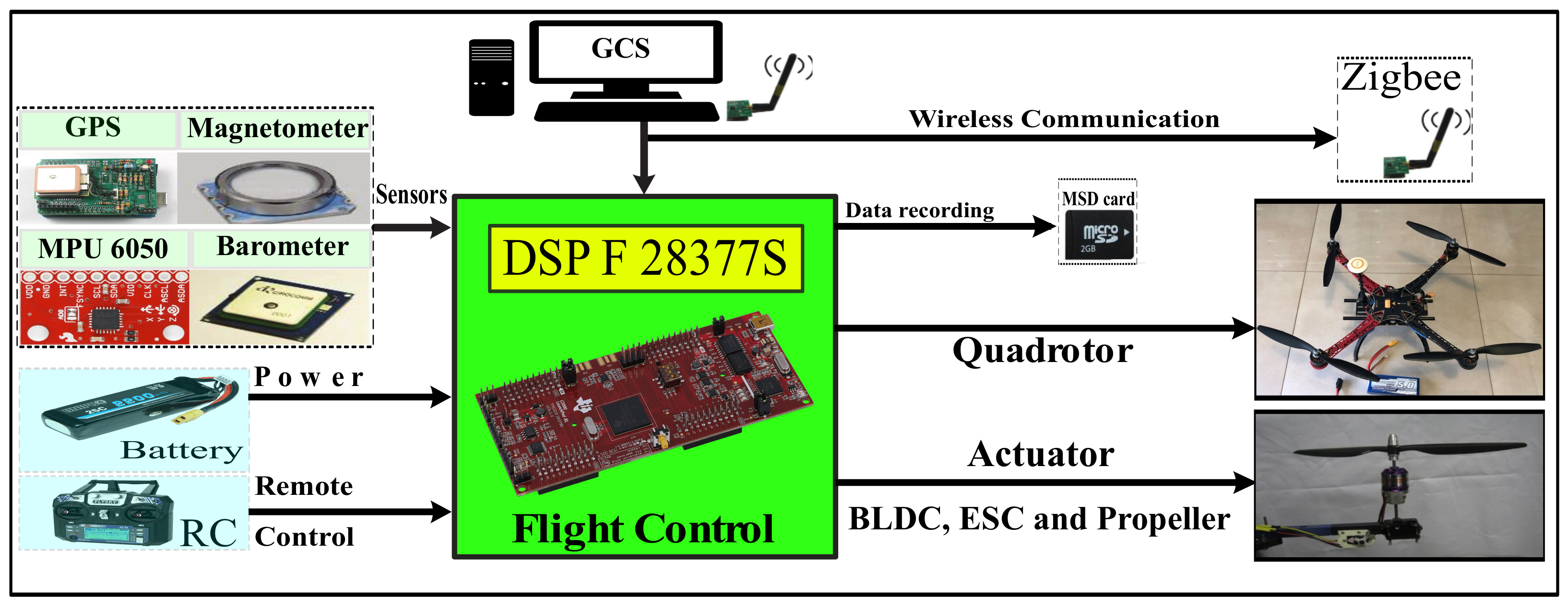
• The Inertial Measurement Unit (IMU) consists of a gyroscope, a three-axis magnetometer, and an accelerometer.
• The GPS module uses horizontal plane measurements to determine the position and velocity. The altitude is measured via a magnetometer and a barometer.
• Communication between the quadrotor and the ground control station (GCS) is ensured by two Zigbee wireless modules.
• Digital signal processing (DSP) is used in the flight control system. The wind is generated by a fan and then applied as an external disturbance to the quadrotor.
• The flight parameters are saved onboard using a micro SD card.

5. Conclusions

The present work introduces a fixed-time fractional-order sliding mode controller for accurate trajectory tracking control of quadrotors with disturbances. A Lyapunov function is created for each subsystem in the quadrotor dynamics to ensure the stability of all the state variables and global stability. Furthermore, the suggested control technique has various advantages over existing controllers, such as higher control precision, fast state variable convergence, and faster tracking performance. Finally, the numerical simulation results demonstrate that the proposed technique FTFOSMC has excellent effectiveness compared to the BSMC and FOSMC methods. For the study of quadrotors that are subject to external disturbances, the comparison to the conventional versions of SMC shows that higher performances can be obtained based on the FTFOSMC, including faster convergence speed for fractional operators, reduced overshoot, weaker error, and lower chattering impact. For future work, the proposed control FTFOSMC will be validated by experiments. Also, the fault-tolerant control problem of the quadrotor will be treated.

References

1. Lu, K.; Xia, Y. Adaptive attitude tracking control for rigid spacecraft with finite-time convergence. Automatica 2013, 49, 3591–3599. [Google Scholar] [CrossRef]
2. Xu, B. Composite learning finite-time control with application to quadrotors. IEEE Trans. Syst. Man Cybern. Syst. 2018, 48, 1806–1815. [Google Scholar] [CrossRef]
3. Polyakov, A. Nonlinear feedback design for fixed-time stabilization of linear control systems. IEEE Trans. Autom. Control 2012, 57, 2106–2110. [Google Scholar] [CrossRef]
4. Labbadi, M.; Cherkaoui, M. Adaptive Fractional-Order Nonsingular Fast Terminal Sliding Mode Based Robust Tracking Control of Quadrotor UAV With Gaussian Random Disturbances and Uncertainties. IEEE Trans. Aerosp. Electron. Syst. 2021, 57, 2265–2277. [Google Scholar] [CrossRef]
5. Labbadi, M.; Boukal, Y.; Cherkaoui, M.; Djemai, M. Fractional-order global sliding mode controller for an uncertain quadrotor UAVs subjected to external disturbances. J. Frankl. Inst. 2021, 358, 4822–4847. [Google Scholar] [CrossRef]
6. Labbadi, M.; Boubaker, S.; Djemai, M.; Mekni, S.K.; Bekrar, A. Fixed-Time Fractional-Order Global Sliding Mode Control for Nonholonomic Mobile Robot Systems under External Disturbances. Fractal Fract. 2022, 6, 177. [Google Scholar] [CrossRef]
7. Liu, D.; Li, T.; He, X. Fixed-Time Multi-Switch Combined–Combined Synchronization of Fractional-Order Chaotic Systems with Uncertainties and External Disturbances. Fractal Fract. 2023, 7, 281. [Google Scholar] [CrossRef]
8. Idrissi, M.; Salami, M.; Annaz, F. A Review of Quadrotor Unmanned Aerial Vehicles: Applications, Architectural Design and Control Algorithms. J. Intell. Robot. Syst. 2022, 104, 22. [Google Scholar] [CrossRef]
9. Huang, S.; Wang, J. Fixed-time fractional-order sliding mode control for nonlinear power systems. J. Vib. Control 2020, 26, 1425–1434. [Google Scholar] [CrossRef]
10. Chen, L.; Fang, J. Adaptive Continuous Sliding Mode Control for Fractional-order Systems with Uncertainties and Unknown Control Gains. Int. J. Control Autom. Syst. 2022, 20, 1509–1520. [Google Scholar] [CrossRef]
11. Muñoz-Vázquez, A.J.; Fernández-Anaya, G.; Sánchez-Torres, J.D. Adaptive parallel fractional sliding mode control. Int. J. Adapt. Control Signal Process. 2021, 36, 751–759. [Google Scholar] [CrossRef]
12. Nikdel, N.; Badamchizadeh, M.; Azimirad, V. Fractional-order adaptive backstepping control of robotic manipulators in the presence of model uncertainties and external disturbances. IEEE Trans. Ind. Electron. 2016, 63, 6249–6256. [Google Scholar] [CrossRef]
13. Wang, J.; Ma, X.; Li, H.; Tian, B. Self-triggered sliding mode control for distributed formation of multiple quadrotors. J. Frankl. Inst. 2020, 357, 12223–12240. [Google Scholar] [CrossRef]
14. Singh, P.; Gupta, S.; Behera, L.; Verma, N.K.; Nahavandi, S. Perching of Nano-Quadrotor Using Self-Trigger Finite-Time Second-Order Continuous Control. IEEE Syst. J. 2021, 15, 4989–4999. [Google Scholar] [CrossRef]
15. Benaddy, A.; Labbadi, M.; Bouzi, M. Robust flight control for a quadrotor under external disturbances based on generic second order sliding mode control. IFAC-PapersOnLine 2022, 55, 270–275. [Google Scholar] [CrossRef]
16. Giap, V.; Vu, H.; Nguyen, Q.; Huang, S.C. Chattering-free sliding mode control-based disturbance observer for MEMS gyroscope system. Microsyst. Technol. 2022, 28, 1867–1877. [Google Scholar] [CrossRef]
17. Ni, J.; Liu, L.; Liu, C.; Hu, X. Fractional order fixed-time nonsingular terminal sliding mode synchronization and control of fractional order chaotic systems. Nonlinear Dyn. 2017, 89, 2065–2083. [Google Scholar] [CrossRef]
18. Aghababa, M.P. A fractional sliding mode for finite-time control scheme with application to stabilization of electrostatic and electromechanical transducers. Appl. Math. Model. 2015, 39, 6103–6113. [Google Scholar] [CrossRef]
19. Lee, J.; Haddad, W.M. Fixed time stability and optimal stabilisation of discrete autonomous systems. Int. J. Control 2022, 96, 2341–2355. [Google Scholar] [CrossRef]
20. Olguin-Roque, J.; Salazar, S.; Gonzalez-Hernandez, I.; Lozano, R. A Robust Fixed-Time Sliding Mode Control for Quadrotor UAV. Algorithms 2023, 16, 229. [Google Scholar] [CrossRef]
21. Giap, V.N.; Nguyen, Q.D.; Trung, N.K.; Huang, S.C. Time-varying disturbance observer based on sliding-mode observer and double phases fixed-time sliding mode control for a T-S fuzzy micro-electro-mechanical system gyroscope. J. Vib. Control 2022, 29, 1927–1942. [Google Scholar] [CrossRef]
22. Ni, J.; Liu, L.; Liu, C.; Hu, X.; Li, S. Fast Fixed-Time Nonsingular Terminal Sliding Mode Control and Its Application to Chaos Suppression in Power System. IEEE Trans. Circuits Syst. II Express Briefs 2017, 64, 151–155. [Google Scholar] [CrossRef]
23. Su, Y. Comments on “Fixed-time sliding mode control with mismatched disturbances” [Automatica 136 (2022) 110009]. Automatica 2023, 151, 110916. [Google Scholar] [CrossRef]
24. Wang, Z.; Wang, J.; Scala, M.L. A Novel Distributed-Decentralized Fixed-Time Optimal Frequency and Excitation Control Framework in a Nonlinear Network-Preserving Power System. IEEE Trans. Power Syst. 2021, 36, 1285–1297. [Google Scholar] [CrossRef]
25. Zeng, T.; Ren, X.; Zhang, Y. Fixed-Time Sliding Mode Control and High-Gain Nonlinearity Compensation for Dual-Motor Driving System. IEEE Trans. Ind. Informatics 2020, 16, 4090–4098. [Google Scholar] [CrossRef]
26. Shirkavand, M.; Pourgholi, M. Robust fixed-time synchronization of fractional order chaotic using free chattering nonsingular adaptive fractional sliding mode controller design. Chaos Solitons Fractals 2018, 113, 135–147. [Google Scholar] [CrossRef]
27. Muñoz-Vázquez, A.J.; Fernández-Anaya, G.; Sánchez-Torres, J.D.; Meléndez-Vázquez, F. Predefined-time control of distributed-order systems. Nonlinear Dyn. 2021, 103, 2689–2700. [Google Scholar] [CrossRef]
28. Huang, S.; Xiong, L.; Wang, J.; Li, P.; Wang, Z.; Ma, M. Fixed-Time Fractional-Order Sliding Mode Controller for Multimachine Power Systems. IEEE Trans. Power Syst. 2021, 36, 2866–2876. [Google Scholar] [CrossRef]
29. Podlubny, I.; Ivo, P.; Blas, M.; Paul, O.; Dorcak, L. Analogue realizations of fractional-order controllers. Nonlinear Dyn. 2002, 29, 281–296. [Google Scholar] [CrossRef]
30. Asignacion, A.; Suzuki, S.; Noda, R.; Nakata, T.; Liu, H. Frequency-Based Wind Gust Estimation for Quadrotors Using a Nonlinear Disturbance Observer. IEEE Robot. Autom. Lett. 2022, 7, 9224–9231. [Google Scholar] [CrossRef]
31. Sanchez-Cuevas, P.; Heredia, G.; Ollero, A. Characterization of the Aerodynamic Ground Effect and Its Influence in Multirotor Control. Int. J. Aerosp. Eng. 2017, 2017, 1823056. [Google Scholar] [CrossRef]
32. Dong, X.; Zhou, Y.; Ren, Z.; Zhong, Y. Time-Varying Formation Tracking for Second-Order Multi-Agent Systems Subjected to Switching Topologies With Application to Quadrotor Formation Flying. IEEE Trans. Ind. Electron. 2017, 64, 5014–5024. [Google Scholar] [CrossRef]
Figure 1. Structure of a quadrotor UAV.
Fractalfract 07 00775 g001
Figure 2. Hierarchical control structure for quadrotor UAV.
Fractalfract 07 00775 g002
Figure 3. Quadrotor position without disturbances.
Fractalfract 07 00775 g003
Figure 4. Quadrotor attitude without disturbances.
Fractalfract 07 00775 g004
Figure 5. Quadrotor inputs without disturbances.
Fractalfract 07 00775 g005
Figure 6. Quadrotor position with disturbances.
Fractalfract 07 00775 g006
Figure 7. Quadrotor attitude with disturbances.
Fractalfract 07 00775 g007
Figure 8. Quadrotor inputs with disturbances.
Fractalfract 07 00775 g008
Figure 9. Quadrotor 3D trajectory with disturbances.
Fractalfract 07 00775 g009
Figure 10. The quadrotor hardware design.
Fractalfract 07 00775 g010