The Analytical Stochastic Solutions for the Stochastic Potential Yu–Toda–Sasa–Fukuyama Equation with Conformable Derivative Using Different Methods

Abstract

We consider in this study the (3+1)-dimensional stochastic potential Yu–Toda–Sasa–Fukuyama with conformable derivative (SPYTSFE-CD) forced by white noise. For different kind of solutions of SPYTSFE-CD, including hyperbolic, rational, trigonometric and function, we use He’s semi-inverse and improved $(G^{\prime }/G)$-expansion methods. Because it investigates solitons and nonlinear waves in dispersive media, plasma physics and fluid dynamics, the potential Yu–Toda–Sasa–Fukuyama theory may explain many intriguing scientific phenomena. We provide numerous 2D and 3D figures to address how the white noise destroys the pattern formation of the solutions and stabilizes the solutions of SPYTSFE-CD.

1. Introduction

The potential Yu–Toda–Sasa–Fukuyama equation (PYTSFE) [1,2] is an intriguing mathematical model that has drawn the attention of researchers for its uses in different fields of science. It combines the Yu–Toda equation, which describes the motion of particles in a one-dimensional lattice, and the Sasa–Fukuyama equation, which models the collective behavior of particles in a non-equilibrium system. By incorporating elements from the potential equation, which characterizes the interactions between particles, the PYTSFE provides a more comprehensive and accurate description of complex systems.

One of the key strengths of the PYTSFE is its versatility and applicability across a range of scientific disciplines. It has found applications in condensed matter physics, statistical mechanics, and even in the study of social networks and biological systems. Its ability to describe the behavior of complex systems, where interactions and dynamics play a crucial role, makes it a valuable tool for understanding real-world phenomena.

The (3+1)-dimensional PYTSFE takes the following form:

$$-4{\mathcal{V}}_{xt}+{\mathcal{V}}_{xxxz}+4{\mathcal{V}}_x{\mathcal{V}}_{xz}+2{\mathcal{V}}_{xx}{\mathcal{V}}_z+3{\mathcal{V}}_{yy}=0,$$

(1)

where $\mathcal{V}(x,y,z,t)$ explains the interfacial wave in a two-layer liquid. Many authors have acquired the analytical solutions of Equation (1), such as the homogeneous balance method [2], bilinear Bäcklund transformations [3], homoclinic test approach [4,5], Hirota bilinear method [6,7], direct method [8], $(G^{\prime }/G)$-expansion method [9], etc.

Moreover, the importance of adding a stochastic term into the PYTSFE brings several important benefits. It allows for the inclusion of inherent randomness, enables the exploration of multiple system states, facilitates the analysis of stability and robustness and facilitates the calibration and validation of the model against the experimental data. By incorporating a stochastic term, the PYTSFE becomes a more realistic and accurate representation of the complex behavior observed in various natural phenomena. Therefore, it is crucial to consider and incorporate stochasticity to enhance the reliability and applicability of the PYTSFE in diverse scientific and engineering disciplines.

On the other side, the study of the fractional potential Yu–Toda–Sa equation is an important area of research in mathematical physics. This equation combines concepts from fractional calculus, potential theory, and soliton theory to provide a powerful tool for understanding physical phenomena with long-range interactions and memory effects. Its applications range from modeling electromagnetic fields in fractal media to describing the dynamics of Bose–Einstein condensates and studying wave propagation in nonlocal media. Recently, authors have been concentrating on fractional calculus and establishing new operators, such as the Caputo, Atangana Baleanu, Caputo Fabrizio, Riemann Liouville, derivatives, He’s fractional derivative and Hadamard [10,11,12,13,14,15,16]. Most fractional derivative forms do not conform to conventional derivative equations including the product rule, mean value theorem, chain rule, quotient rule, Rolle’s theorem and chain rule. As a result, Khalil et al. [17] presented a new derivative called the conformable derivative (CD), which is a natural extension of the classical derivative. Khalil et al. [17] defined the CD of order $\delta$ for the function $\mathsf{\Psi }:{\mathbb{R}}^{+}\to \mathbb{R}$ as follows:

$${\mathbb{T}}_x^{\delta }\mathsf{\Psi }\left(x\right)=\underset{h\to 0}{lim}\frac{\mathsf{\Psi }(x+h{x}^{1-\delta })-\mathsf{\Psi }\left(x\right)}{h}.$$

As a result, it is important to consider here the stochastic potential Yu–Toda–Sasa–Fukuyama equation with conformable derivative (SPYTSFE-CD) as follows:

$$-4d\left[{\mathbb{T}}_x^{\delta }\mathcal{V}\right]+[{\mathbb{T}}_{xxxz}^{\delta }\mathcal{V}+4{\mathbb{T}}_x^{\delta }\mathcal{V}{\mathbb{T}}_{xz}^{\delta }\mathcal{V}+2{\mathbb{T}}_{xx}^{\delta }\mathcal{V}{\mathbb{T}}_z^{\delta }\mathcal{V}+3{\mathbb{T}}_{yy}^{\delta }\mathcal{V}]dt+4\sigma {\mathbb{T}}_x^{\delta }\mathcal{V}d\mathcal{W}=0,$$

(2)

where $\mathcal{W}=\mathcal{W}\left(t\right)$ is a white noise and $\sigma$ represents the noise amplitude.

Our novelty in this study is to obtain the exact stochastic solutions of SPYTSFE-CD (2). To obtain different types of solutions, including hyperbolic, rational, trigonometric and function, we apply two various methods such as He’s semi-inverse and improved $(G^{\prime }/G)$-expansion methods. Due to the existence of the stochastic term and conformable derivative operator in Equation (2), the derived solutions are very useful for describing various essential physical phenomena, and physicists should take them into account. Furthermore, we generalize some earlier obtained results, including those stated in [8]. Finally, we introduce many graphs by utilizing MATLAB tools to discuss the impact of noise and the conformable derivative on the solution of SPYTSFE-CD (2).

This research is summarized as follows: Section 2 investigates the SPYTSFE-CD wave equation. Section 3 concentrates on exact solutions for the SPYTSFE-CD. In Section 4, we investigate how Brownian motion impacts solutions of SPYTSFE-CD. The conclusions of this study are stated in the end.

2. Wave Equation for SPYTSFE

To obtain the wave equation for SPYTSFE-CD (2), we use

$$\mathcal{V}(x,y,z,t)=\mathcal{U}\left(\eta \right)e^{(\sigma \mathcal{W}\left(t\right)-\frac{1}{2}{\sigma }^{2}t)},\eta =\frac{{\eta }_1}{\delta }{x}^{\delta }+\frac{{\eta }_2}{\delta }{y}^{\delta }+\frac{{\eta }_3}{\delta }{z}^{\delta }+{\eta }_{4}t,$$

(3)

where the function $\mathcal{U}$ is deterministic; ${\eta }_1,{\eta }_2,$${\eta }_3$ are the wave frequency; and ${\eta }_4$ is the wave speed. We observe that

$$\begin{array}{ccc}\hfill {\mathbb{T}}_x^{\delta }\mathcal{V}& =& {\eta }_1{\mathcal{U}}^{\prime }{e}^{(\sigma \mathcal{W}\left(t\right)-\frac{1}{2}{\sigma }^{2}t)},{\mathbb{T}}_z^{\delta }\mathcal{V}={\eta }_3{\mathcal{U}}^{\prime }{e}^{(\sigma \mathcal{W}\left(t\right)-\frac{1}{2}{\sigma }^{2}t)},\hfill \\ \hfill {\mathbb{T}}_{xz}^{\delta }\mathcal{V}& =& {\eta }_1{\eta }_3{\mathcal{U}}^{″}{e}^{(\sigma \mathcal{W}\left(t\right)-\frac{1}{2}{\sigma }^{2}t)},{\mathbb{T}}_{xx}^{\delta }\mathcal{V}={\eta }_1^2{\mathcal{U}}^{″}{e}^{(\sigma \mathcal{W}\left(t\right)-\frac{1}{2}{\sigma }^{2}t)},\hfill \\ \hfill {\mathbb{T}}_{yy}^{\delta }\mathcal{V}& =& {\eta }_2^2{\mathcal{U}}^{″}{e}^{(\sigma \mathcal{W}\left(t\right)-\frac{1}{2}{\sigma }^{2}t)},{\mathbb{T}}_{xxxz}^{\delta }\mathcal{V}={\eta }_3{\eta }_1^3{\mathcal{U}}^{″″}{e}^{(\sigma \mathcal{W}\left(t\right)-\frac{1}{2}{\sigma }^{2}t)},\hfill \\ \hfill d\left[{\mathbb{T}}_x^{\delta }\mathcal{V}\right]& =& [{\eta }_1{\eta }_4{\mathcal{U}}^{″}dt+\sigma {\eta }_1{\mathcal{U}}^{\prime }d\mathcal{W}]e^{(\sigma \mathcal{W}\left(t\right)-\frac{1}{2}{\sigma }^{2}t)}.\hfill \end{array}$$

(4)

Inserting Equation (4) into Equation (2) yields

$$(3{\eta }_2^2-4{\eta }_1{\eta }_4){\mathcal{U}}^{″}+{\eta }_3{\eta }_1^3{\mathcal{U}}^{″″}+6{\eta }_3{\eta }_1^2{\mathcal{U}}^{\prime }{\mathcal{U}}^{″}{e}^{(\sigma \mathcal{W}\left(t\right)-\frac{1}{2}{\sigma }^{2}t)}=0.$$

(5)

When we take the expectations $\mathbb{E}(·)$ on both sides, we obtain

$$(3{\eta }_2^2-4{\eta }_1{\eta }_4){\mathcal{U}}^{″}+{\eta }_3{\eta }_1^3{\mathcal{U}}^{″″}+6{\eta }_3{\eta }_1^2{\mathcal{U}}^{\prime }{\mathcal{U}}^{″}{e}^{-\frac{1}{2}{\sigma }^{2}t}\mathbb{E}{e}^{\left(\sigma \mathcal{W}\right(t\left)\right)}=0.$$

(6)

Since $\mathcal{W}\left(t\right)$ is Normal distribution, then $\mathbb{E}\left(e^{\sigma \mathcal{W}\left(t\right)}\right)=e^{\left(\frac{1}{2}{\sigma }^{2}t\right)}$, Equation (6) turns into

$${\ell }_1{\mathcal{U}}^{″}+{\mathcal{U}}^{″″}+2{\ell }_2{\mathcal{U}}^{\prime }{\mathcal{U}}^{″}=0,$$

(7)

where

$${\ell }_1=\frac{(3{\eta }_2^2-4{\eta }_1{\eta }_4)}{{\eta }_3{\eta }_1^3}\mathrm{and}{\ell }_2=\frac{3}{{\eta }_1}.$$

(8)

Integrating Equation (7) and ignoring the constant of the integral yields

$${\mathcal{U}}^{‴}+{\ell }_1{\mathcal{U}}^{\prime }+{\ell }_2{\left({\mathcal{U}}^{\prime }\right)}^2=0.$$

(9)

3. Exact Solutions of SPYTSFE

He’s semi-inverse and improved $(G^{\prime }/G)$-expansion methods are applied to solve the wave Equation (9). After that, SPYTSFE (2) solutions are identified.

3.1. He’s Semi-Inverse Method

We derive, by applying He’s semi-inverse method [18,19,20], the variational formulations:

$$\mathbb{J}\left(\mathcal{U}\right)={\int }_0^{\infty }\{\frac{1}{2}{\left({\mathcal{U}}^{″}\right)}^2-\frac{1}{2}{\ell }_1{\left({\mathcal{U}}^{\prime }\right)}^2+\frac{1}{3}{\ell }_2{\left({\mathcal{U}}^{\prime }\right)}^3\}d\eta .$$

(10)

Using the format specified by [21], we assume the solution of (7) is

$$\mathcal{U}\left(\eta \right)=\mathcal{K}\mathrm{sech}\left(\eta \right),$$

(11)

where $\mathcal{K}$ is an undefined constant. Inserting Equation (11) into Equation (10) yields

$$\begin{array}{ccc}\hfill \mathbb{J}& =& \frac{1}{2}{\mathcal{K}}^2{\int }_0^{\infty }[{\mathrm{sech}}^2\left(\eta \right){tanh}^4\left(\eta \right)+{\mathrm{sech}}^4\left(\eta \right){tanh}^2\left(\eta \right)+{\mathrm{sech}}^6\left(\eta \right)\hfill \\ & & -{\ell }_1{\mathrm{sech}}^2\left(\eta \right){tanh}^2\left(\eta \right)+\frac{2}{3}{\ell }_2\mathcal{K}{\mathrm{sech}}^3\left(\eta \right){tanh}^3\left(\eta \right)]d\eta \hfill \\ & =& \frac{1}{2}{\mathcal{K}}^2{\int }_0^{\infty }[{\mathrm{sech}}^2\left(\eta \right)-{\ell }_1{\mathrm{sech}}^2\left(\eta \right){tanh}^2\left(\eta \right)+\frac{2}{3}{\ell }_2\mathcal{K}{\mathrm{sech}}^3\left(\eta \right){tanh}^3\left(\eta \right)]d\eta \hfill \\ & =& \frac{{\mathcal{K}}^2}{2}-{\ell }_1\frac{{\mathcal{K}}^2}{6}-\frac{2}{45}{\ell }_2{\mathcal{K}}^3.\hfill \end{array}$$

Putting $\frac{\partial \mathbb{J}}{\partial \mathcal{K}}=0$ as follows

$$\frac{\partial \mathbb{J}}{\partial \mathcal{K}}=(1-\frac{1}{3}{\ell }_1)\mathcal{K}-\frac{2}{15}{\ell }_2{\mathcal{K}}^2=0.$$

(12)

By solving Equation (12), we obtain

$$\mathcal{K}=\frac{15-5{\ell }_1}{2{\ell }_2}.$$

Hence, Equation (7) has the solution

$$\mathcal{U}\left(\eta \right)=\frac{15-5{\ell }_1}{6{\ell }_2}\mathrm{sech}\left(\eta \right).$$

Now, the solution of SPYTSFE (2) is

$$\mathcal{V}(x,y,z,t)=\frac{15-5{\ell }_1}{6{\ell }_2}\mathrm{sech}(\frac{{\eta }_1}{\delta }{x}^{\delta }+\frac{{\eta }_2}{\delta }{y}^{\delta }+\frac{{\eta }_3}{\delta }{z}^{\delta }+{\eta }_{4}t)e^{(\sigma \mathcal{W}\left(t\right)-\frac{1}{2}{\sigma }^{2}t)}.$$

(13)

Similarly, we use the identical procedure for the solution of Equation (7) as

$$\mathcal{U}\left(\eta \right)=\mathcal{N}\mathrm{sech}\left(\eta \right){tanh}^2\left(\eta \right).$$

We obtain the following by repeating the preceding steps:

$$\mathcal{N}=\frac{11(1199-213{\ell }_1)}{1456{\ell }_2}.$$

Thus, the solution of SPYTSFE-CD (2) is

$$\mathcal{V}(x,y,z,t)=\frac{11(1199-213{\ell }_1)}{1456{\ell }_2}\mathrm{sech}\left(\eta \right){tanh}^2\left(\eta \right)e^{(\sigma \mathcal{W}\left(t\right)-\frac{1}{2}{\sigma }^{2}t)},$$

(14)

where $\eta =\frac{{\eta }_1}{\delta }{x}^{\delta }+\frac{{\eta }_2}{\delta }{y}^{\delta }+\frac{{\eta }_3}{\delta }{z}^{\delta }+{\eta }_{4}t.$

3.2. Improved $(G^{\prime }/G)$-Expansion Method

Supposing that the solution $\mathcal{U}$ of Equation (9) takes the type

$$\mathcal{U}\left(\eta \right)=A_0+\sum _{k=1}^N{A}_k{[\frac{G^{\prime }}{G}]}^k,$$

(15)

where $A_k$ is constant for $k=0,1,2,\dots ,N$ such that $A_N\ne 0$ and G solves

$${\left[G^{\prime }\right]}^2=\alpha G^2+\beta G^4+\gamma G^6,$$

(16)

since $\alpha ,\beta$ and $\gamma$ are undefined constants to be evaluated later. Equation (16) has the following solutions [22,23]:

No	$\mathbf{G}\left(\mathit{\eta }\right)=$
1	${\left[\frac{-\alpha \beta {\mathrm{sech}}^2\left(\sqrt{\alpha }\eta \right)}{{\beta }^2-\alpha \gamma {(1\pm tanh\left(\sqrt{\alpha }\eta \right))}^2}\right]}^{1/2}$or${\left[\frac{-\alpha \beta {\mathrm{csch}}^2\left(\sqrt{\alpha }\eta \right)}{{\beta }^2-\alpha \gamma {(1\pm coth\left(\sqrt{\alpha }\eta \right))}^2}\right]}^{1/2}$if$\alpha >0,$
2	${\left[\frac{2\alpha }{\pm \sqrt{\Delta }cosh\left(2\sqrt{\alpha }\eta \right)-\beta }\right]}^{1/2}$if$\alpha >0$and $\Delta >0,$
3	${\left[\frac{2\alpha }{\pm \sqrt{\Delta }cos\left(2\sqrt{-\alpha }\eta \right)-\beta }\right]}^{1/2}$or${\left[\frac{2\alpha }{\pm \sqrt{\Delta }sin\left(2\sqrt{-\alpha }\eta \right)-\beta }\right]}^{1/2}$if$\alpha <0$and $\Delta >0,$
4	${\left[\frac{2\alpha }{\pm \sqrt{-\Delta }sinh\left(2\sqrt{\alpha }\eta \right)-\beta }\right]}^{1/2}$if$\alpha >0$and $\Delta <0,$
5	${\left[\frac{-\alpha {\mathrm{sech}}^2\left(\sqrt{\alpha }\eta \right)}{{\beta }^2\pm 2\sqrt{\alpha \gamma }tanh\left(\sqrt{\alpha }\eta \right)}\right]}^{1/2}$or${\left[\frac{-\alpha {\mathrm{csch}}^2\left(\sqrt{\alpha }\eta \right)}{{\beta }^2\pm 2\sqrt{\alpha \gamma }coth\left(\sqrt{\alpha }\eta \right)}\right]}^{1/2}$if$\alpha >0$and $\gamma >0,$
6	${\left[\frac{-\alpha {sec}^2\left(\sqrt{-\alpha }\eta \right)}{{\beta }^2\pm 2\sqrt{-\alpha \gamma }tan\left(\sqrt{-\alpha }\eta \right)}\right]}^{1/2}$or${\left[\frac{-\alpha {csc}^2\left(\sqrt{-\alpha }\eta \right)}{{\beta }^2\pm 2\sqrt{-\alpha \gamma }cot\left(\sqrt{-\alpha }\eta \right)}\right]}^{1/2}$if$\alpha <0$and $\gamma >0,$
7	${\left[\frac{\alpha e^{\pm \left(2\sqrt{\alpha }\eta \right)}}{(e^{\pm {(2\sqrt{\alpha }\eta -4\beta )}^2}-64\alpha \gamma }\right]}^{1/2}$if$\alpha >0,$
8	$-\frac{\alpha }{\beta }{\left[1\pm tanh\left(\frac{1}{2}\sqrt{\alpha }\eta \right)\right]}^{1/2}$or$-\frac{\alpha }{\beta }{\left[1\pm coth\left(\frac{1}{2}\sqrt{\alpha }\eta \right)\right]}^{1/2}$if$\alpha >0$and $\Delta =0,$
9	${\left[\frac{\pm \alpha e^{\pm \left(2\sqrt{\alpha }\eta \right)}}{1-64\alpha \gamma e^{\pm \left(4\sqrt{\alpha }\eta \right)}}\right]}^{1/2}$if$\alpha >0,$ and $\beta =0,$
10	$\pm \frac{1}{\sqrt{\beta }\eta }$if$\alpha =0,$ and $\gamma =0,$
where $\Delta ={\beta }^2-4\alpha \gamma .$

By utilizing homogeneous balancing between ${\mathcal{U}}^{‴}$ with ${\left({\mathcal{U}}^{\prime }\right)}^2$ in Equation (9), we have

$$2N+2=N+3⟹N=1.$$

Then, Equation (15) turns into

$$\mathcal{U}\left(\eta \right)=A_0+A_1\frac{G^{\prime }}{G}.$$

(17)

Plugging Equation (17) into Equation (9), use

$${\mathcal{U}}^{\prime }\left(\eta \right)=A_1[\beta G^2+2\gamma G^4],$$

and

$${\mathcal{U}}^{‴}\left(\eta \right)=A_1[4\alpha \beta G^2+(6{\beta }^2+32\alpha \gamma )G^4+48\gamma \beta G^6+24{\gamma }^2{G}^8],$$

in order to obtain

$$\begin{array}{c} (24{\gamma }^2{A}_1+4{\ell }_2{\gamma }^2{A}_1^2)G^8+\gamma \beta A_1(48+4{\ell }_2)G^6+\hfill \\ +A_1(6{\beta }^2+32\alpha \gamma +2\gamma {\ell }_1+{\beta }^2{\ell }_2{A}_1)G^4+\beta A_1(4\alpha +{\ell }_1)G^2=0.\hfill \end{array}$$

Putting each coefficients $G^k$ to zero, we have

$$\begin{array}{c}24{\gamma }^2{A}_1+4{\ell }_2{\gamma }^2{A}_1^2=0,\\ \gamma \beta A_1(48+4{\ell }_2)=0,\\ A_1(6{\beta }^2+32\alpha \gamma +2\gamma {\ell }_1+{\beta }^2{\ell }_2{A}_1)=0,\end{array}$$

and

$$\beta A_1(4\alpha +{\ell }_1)=0.$$

When we solve the above equations, we acquire the following sets:

First set:

$$A_0=\mathrm{Free},A_1=\frac{-6}{{\ell }_2},\gamma =\mathrm{Free},\beta =0,\mathrm{and}{\eta }_4=\frac{(3{\eta }_2^2+16\alpha {\eta }_3{\eta }_1^3)}{4{\eta }_1}.$$

(18)

Second set:

$$A_0=\mathrm{Free},A_1=\frac{-6}{{\ell }_2},\gamma =0,\beta =\mathrm{Free},\mathrm{and}{\eta }_4=\frac{(3{\eta }_2^2+4\alpha {\eta }_3{\eta }_1^3)}{4{\eta }_1}.$$

(19)

First set: Equation (9) possesses the solution

$$\mathcal{U}\left(\eta \right)=A_0-2{\eta }_1\frac{G^{\prime }}{G},\mathrm{with}\beta =0,$$

(20)

where $\eta =\frac{{\eta }_1}{\delta }{x}^{\delta }+\frac{{\eta }_2}{\delta }{y}^{\delta }+\frac{{\eta }_3}{\delta }{z}^{\delta }+\frac{(3{\eta }_2^2+16\alpha {\eta }_3{\eta }_1^3)}{4{\eta }_1}t.$

There are several cases based on $\alpha$ and $\gamma$:

Case-1: When $\alpha >0$ and $\gamma <0,$ Equation (16) possesses the solution

$$G\left(\eta \right)={\left[\sqrt{\frac{-\alpha }{\gamma }}\mathrm{sech}\left(2\sqrt{\alpha }\eta \right)\right]}^{1/2}.$$

Therefore, the solution (20) is

$$\mathcal{U}\left(\eta \right)=A_0-2\sqrt{\alpha }{\eta }_{1}tanh\left(2\sqrt{\alpha }\eta \right).$$

Consequently, the solution of SPYTSFE-CD (2) is

$$\mathcal{V}(x,y,z,t)=[A_0-2\sqrt{\alpha }{\eta }_{1}tanh\left(2\sqrt{\alpha }\eta \right)]e^{(\sigma \mathcal{W}\left(t\right)-\frac{1}{2}{\sigma }^{2}t)}.$$

(21)

Case-2: When $\alpha <0$ and $\gamma >0,$ then Equation (16) has the solution

$$G\left(\eta \right)={\left[\sqrt{\frac{-\alpha }{\gamma }}sec\left(2\sqrt{-\alpha }\eta \right)\right]}^{1/2}\mathrm{or}G\left(\eta \right)={\left[\sqrt{\frac{-\alpha }{\gamma }}csc\left(2\sqrt{-\alpha }\eta \right)\right]}^{1/2}.$$

Hence, the solution (20) has the form

$$\mathcal{U}\left(\eta \right)=A_0-2\sqrt{-\alpha }{\eta }_{1}tan\left(2\sqrt{-\alpha }\eta \right)\mathrm{or}\mathcal{U}\left(\eta \right)=A_0+2\sqrt{-\alpha }{\eta }_{1}cot\left(2\sqrt{-\alpha }\eta \right)$$

As a result, the solution to SPYTSFE-CD (2) is

$$\mathcal{V}(x,y,z,t)=[A_0-2\sqrt{-\alpha }{\eta }_{1}tan\left(2\sqrt{-\alpha }\eta \right)]e^{(\sigma \mathcal{W}\left(t\right)-\frac{1}{2}{\sigma }^{2}t)},$$

(22)

or

$$\mathcal{V}(x,y,z,t)=[A_0+2\sqrt{-\alpha }{\eta }_{1}cot\left(2\sqrt{-\alpha }\eta \right)]e^{(\sigma \mathcal{W}\left(t\right)-\frac{1}{2}{\sigma }^{2}t)}.$$

(23)

Case-3: When $\alpha >0$ and $\gamma <0,$ the solution of Equation (16) is

$$G\left(\eta \right)={\left[\sqrt{\frac{-\alpha }{\gamma }}\mathrm{csch}\left(2\sqrt{\alpha }\eta \right)\right]}^{1/2}.$$

Therefore, the solution (20) is

$$\mathcal{U}\left(\eta \right)=A_0-2\sqrt{\alpha }{\eta }_{1}coth\left(2\sqrt{\alpha }\eta \right).$$

Consequently, the solution of SPYTSFE-CD (2) is

$$\mathcal{V}(x,y,z,t)=[A_0+2\sqrt{\alpha }{\eta }_{1}coth\left(2\sqrt{\alpha }\eta \right)]e^{(\sigma \mathcal{W}\left(t\right)-\frac{1}{2}{\sigma }^{2}t)}.$$

(24)

Case-4: When $\alpha >0,$ Equation (16) has the solution

$$G\left(\eta \right)={\left[\frac{\pm \alpha e^{\pm \left(2\sqrt{\alpha }\eta \right)}}{1-64\alpha \gamma e^{\pm \left(4\sqrt{\alpha }\eta \right)}}\right]}^{1/2}.$$

Hence, the solution (20) has the form

$$\mathcal{U}\left(\eta \right)=A_0-2{\eta }_1\frac{\pm \alpha \sqrt{\alpha }{e}^{\pm \left(2\sqrt{\alpha }\eta \right)}(1+64\alpha \gamma e^{\pm \left(4\sqrt{\alpha }\eta \right)})}{{(1-64\alpha \gamma e^{\pm \left(4\sqrt{\alpha }\eta \right)})}^2}.$$

As a result, the solution to SPYTSFE-CD (2) is

$$\mathcal{V}(x,y,z,t)=[A_0-2{\eta }_1\frac{\pm \alpha \sqrt{\alpha }{e}^{\pm \left(2\sqrt{\alpha }\eta \right)}(1+64\alpha \gamma e^{\pm \left(4\sqrt{\alpha }\eta \right)})}{{(1-64\alpha \gamma e^{\pm \left(4\sqrt{\alpha }\eta \right)})}^2}]e^{(\sigma \mathcal{W}\left(t\right)-\frac{1}{2}{\sigma }^{2}t)}.$$

(25)

Second set: Equation (9) possess the solution

$$\mathcal{U}\left(\eta \right)=A_0-2{\eta }_1\frac{G^{\prime }}{G},\mathrm{with}\gamma =0,$$

(26)

where $\eta =\frac{{\eta }_1}{\delta }{x}^{\delta }+\frac{{\eta }_2}{\delta }{y}^{\delta }+\frac{{\eta }_3}{\delta }{z}^{\delta }+\frac{(3{\eta }_2^2+4\alpha {\eta }_3{\eta }_1^3)}{4{\eta }_1}t.$

There are many cases based on $\alpha$ and $\beta$:

Case-1: When $\alpha >0$ and $\beta <0,$ Equation (16) has the solution

$$G\left(\eta \right)=\sqrt{\frac{-\alpha }{\beta }}\mathrm{sech}\left(\sqrt{\alpha }\eta \right)\mathrm{or}G\left(\eta \right)=\sqrt{\frac{-\alpha }{\beta }}\mathrm{csch}\left(\sqrt{\alpha }\eta \right).$$

Therefore, the solution (20) is

$$\mathcal{U}\left(\eta \right)=A_0-2\sqrt{\alpha }{\eta }_{1}tanh\left(\sqrt{\alpha }\eta \right)\mathrm{or}\mathcal{U}\left(\eta \right)=A_0+2\sqrt{\alpha }{\eta }_{1}coth\left(\sqrt{\alpha }\eta \right).$$

As a result, the solution to SPYTSFE-CD (2) is

$$\mathcal{V}(x,y,z,t)=[A_0-2\sqrt{\alpha }{\eta }_{1}tanh\left(\sqrt{\alpha }\eta \right)]e^{(\sigma \mathcal{W}\left(t\right)-\frac{1}{2}{\sigma }^{2}t)},$$

(27)

or

$$\mathcal{V}(x,y,z,t)=[A_0+2\sqrt{\alpha }{\eta }_{1}coth\left(\sqrt{\alpha }\eta \right)]e^{(\sigma \mathcal{W}\left(t\right)-\frac{1}{2}{\sigma }^{2}t)}.$$

(28)

Case-2: If $\alpha >0$ and $\beta >0,$ then Equation (16) has the solution

$$G\left(\eta \right)={\left[\frac{2\alpha }{\pm \beta cosh\left(2\sqrt{\alpha }\eta \right)-\beta }\right]}^{1/2}.$$

Hence, the solution (20) has the form

$$\mathcal{U}\left(\eta \right)=A_0\pm \frac{2\sqrt{\alpha }{\eta }_{1}sinh\left(2\sqrt{\alpha }\eta \right)}{\pm cosh\left(2\sqrt{\alpha }\eta \right)-1}.$$

Consequently, the solution of SPYTSFE-CD (2) is

$$\mathcal{V}(x,y,z,t)=[A_0\pm \frac{2\sqrt{\alpha }{\eta }_{1}sinh\left(2\sqrt{\alpha }\eta \right)}{\pm cosh\left(2\sqrt{\alpha }\eta \right)-1}]e^{(\sigma \mathcal{W}\left(t\right)-\frac{1}{2}{\sigma }^{2}t)}.$$

(29)

Case-3: If $\alpha <0$ and $\beta >0,$ then Equation (16) has the solution

$$G\left(\eta \right)={\left[\frac{2\alpha }{\pm \beta cos\left(2\sqrt{-\alpha }\eta \right)-\beta }\right]}^{1/2}\mathrm{or}G\left(\eta \right)={\left[\frac{2\alpha }{\pm \beta sin\left(2\sqrt{-\alpha }\eta \right)-\beta }\right]}^{1/2}.$$

Therefore, the solution (20) is

$$\mathcal{U}\left(\eta \right)=A_0\mp \frac{2\sqrt{-\alpha }{\eta }_{1}sin\left(2\sqrt{-\alpha }\eta \right)}{\pm cos\left(2\sqrt{-\alpha }\eta \right)-1}\mathrm{or}\mathcal{U}\left(\eta \right)=A_0\pm \frac{2\sqrt{-\alpha }{\eta }_{1}cos\left(2\sqrt{-\alpha }\eta \right)}{\pm sin\left(2\sqrt{-\alpha }\eta \right)-1}.$$

As a result, the solution to SPYTSFE-CD (2) is

$$\mathcal{V}(x,y,z,t)=[A_0\mp \frac{2\sqrt{-\alpha }{\eta }_{1}sin\left(2\sqrt{-\alpha }\eta \right)}{\pm cos\left(2\sqrt{-\alpha }\eta \right)-1}]e^{(\sigma \mathcal{W}\left(t\right)-\frac{1}{2}{\sigma }^{2}t)},$$

(30)

or

$$\mathcal{V}(x,y,z,t)=[A_0\pm \frac{2\sqrt{\alpha }{\eta }_{1}cos\left(2\sqrt{-\alpha }\eta \right)}{\pm sin\left(2\sqrt{-\alpha }\eta \right)-1}]e^{(\sigma \mathcal{W}\left(t\right)-\frac{1}{2}{\sigma }^{2}t)}.$$

(31)

Case-4: If $\alpha >0,$ then Equation (16) has the solution

$$G\left(\eta \right)={\left[\frac{\alpha e^{\pm \left(2\sqrt{\alpha }\eta \right)}}{e^{\pm \left(2\sqrt{\alpha }\eta \right){-4\beta )}^2}}\right]}^{1/2}.$$

Hence, the solution (20) has the form

$$\mathcal{U}\left(\eta \right)=A_0\pm 2\alpha {\eta }_1.$$

Consequently, the solution of SPYTSFE-CD (2) is

$$\mathcal{V}(x,y,z,t)=[A_0\pm 2\alpha {\eta }_1]e^{(\sigma \mathcal{W}\left(t\right)-\frac{1}{2}{\sigma }^{2}t)}.$$

(32)

Case-5: When $\alpha =0,$ Equation (16) has the solution

$$G\left(\eta \right)=\pm \frac{1}{\sqrt{\beta }\eta }.$$

Therefore, the solution (20) is

$$\mathcal{U}\left(\eta \right)=A_0+2{\eta }_1\frac{1}{\eta }.$$

As a result, the solution to SPYTSFE-CD (2) is

$$\mathcal{V}(x,y,z,t)=[A_0+2{\eta }_1\frac{1}{\eta }]e^{(\sigma \mathcal{W}\left(t\right)-\frac{1}{2}{\sigma }^{2}t)}.$$

(33)

Remark 1.

If we set $\sigma =0$ and $\delta =1$ in Equations (22), (23), (27) and (28), then we obtain the same results (34), (35), (28), and (29), respectively, that are reported in [8].

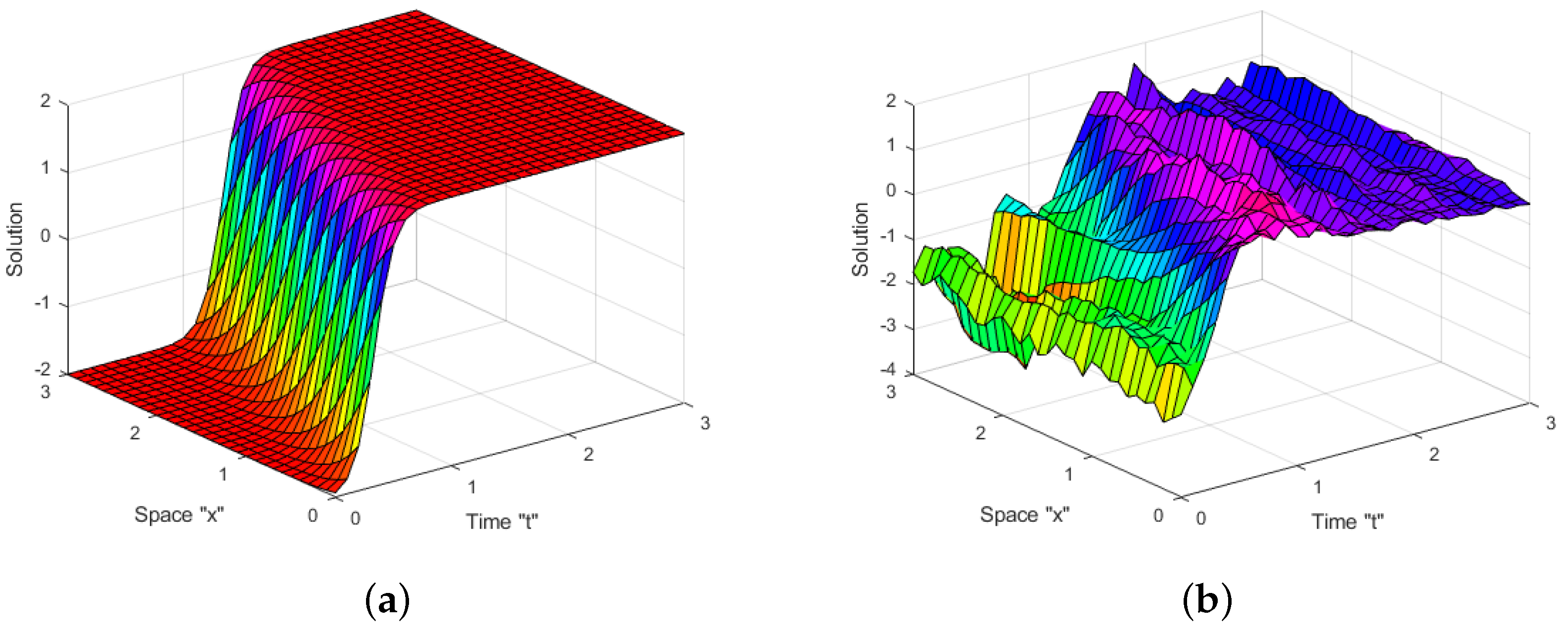
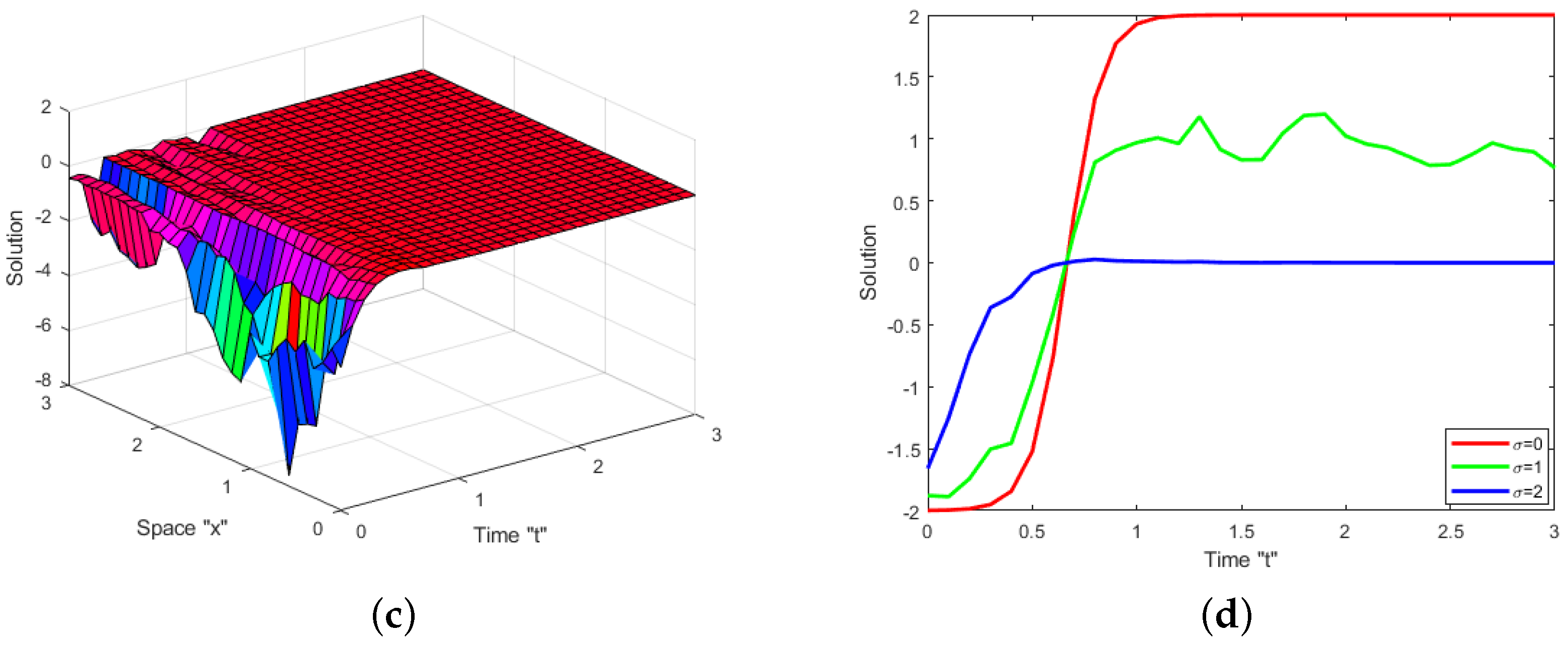
4. Impacts of White Noise and CD

Here, we examine the impact of white noise and CD on the acquired solutions.

4.1. Impact of White Noise

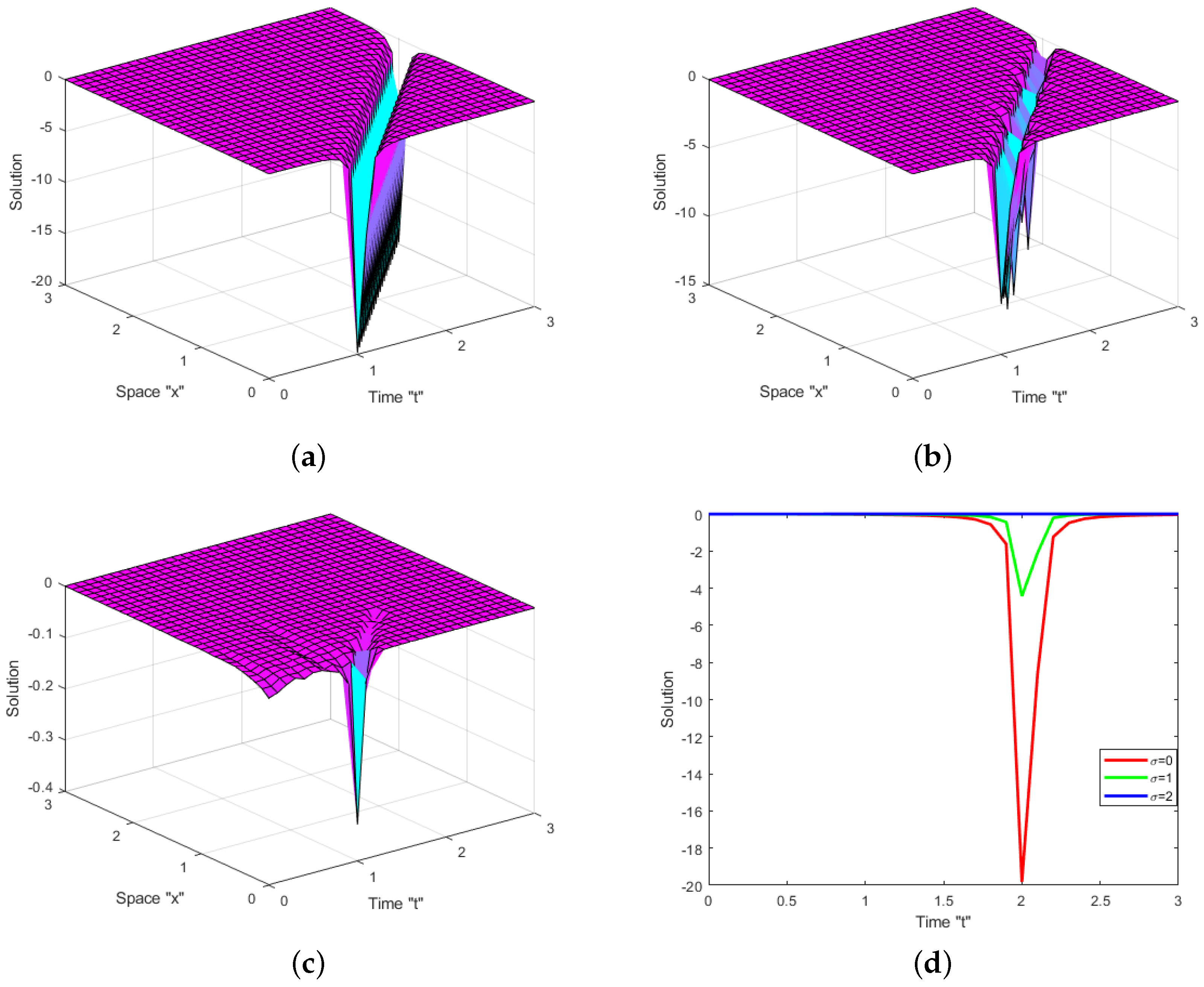
White noise can significantly impact the solutions of differential equations. When solving these equations, one aims to find a function that satisfies the given differential equation. However, the presence of white noise in the system can introduce random fluctuations, making it challenging to obtain such solutions. The noise acts as a disturbance that disrupts the equilibrium state of the system, leading to more unpredictable results. Therefore, when dealing with differential equations, it is crucial to account for the potential effect of white noise to ensure accurate solutions.

Furthermore, the effect of white noise on optimization problems cannot be overlooked. Optimization aims to find the best possible solution to a given problem, often by maximizing or minimizing an objective function. However, the presence of white noise can alter the search landscape, making it difficult to identify the optimal solution. The randomness of the noise can cause the optimization algorithm to become stuck in suboptimal regions or erroneously converge on incorrect solutions. As a result, incorporating white noise into optimization algorithms requires careful consideration to ensure the accuracy of the obtained solutions.

We now look at the influence of noise on the attained solutions of the SPYTSFE-CFD (2). Numerous graphs depicting the efficiency of various solutions, such as (14), (21) and (25), are simulated by using the Euler–Maruyama method (for more details about the code, see [24]). The impact of stochastic term on the solutions is shown in the following graphs:

Figure 1, Figure 2 and Figure 3 show that when the noise is absent (i.e., at $\sigma =0$), there are various kinds of solutions. As noise is introduced, the surface gradually becomes flatter after a few little transit patterns. This indicates that the SPYTSFE-CD solutions are impacted by noise and are stabilized around zero.

4.2. Impact of CD

Figure 4 and Figure 5 demonstrate that when the order of derivative decreases, the surface contracts and shifts to the left, as follows:

5. Conclusions

In this study, we took into account the stochastic potential Yu–Toda–Sasa–Fukuyama with conformable derivative (SPYTSFE-CD). By utilizing He’s semi-inverse and improved $(G^{\prime }/G)$-expansion methods, we acquired different types of exact solutions for SPYTSFE-CD (2). Since potential Yu–Toda–Sasa–Fukuyama is used in studying the solitons and nonlinear waves in dispersive media, plasma physics and fluid dynamics, the obtained solutions in this paper may be used to explain a wide variety of exciting physical phenomena. Moreover, we expanded some earlier acquired solutions, including those stated in [8]. Finally, we constructed a large number of 3D and 2D figures to study the impact of the white noise and conformable derivative on the exact solutions of the SPYTSFE-CD. In our next work, we can address Equation (2) with an additive stochastic term.

References

1. Yu, S.; Toda, K.; Sasa, N.; Fukuyama, T. N soliton solutions to the Bogoyavlenskii-Schiff equation and a quest for the soliton solution in (3+1) dimensions. J. Phys. A 1998, 31, 3337–3347. [Google Scholar] [CrossRef]
2. Yan, Z.Y. New families of non-travelling wave solutions to a new (3+1)-dimensional potential-YTSF equation. Phys. Lett. A 2003, 318, 78–83. [Google Scholar] [CrossRef]
3. Yin, H.M.; Tian, B.; Chai, J.; Wu, X.Y.; Sun, W.R. Solitons and bilinear Bäcklund transformations for a (3+1) mathcontainer loading mathjax-dimensional Yu–Toda–Sasa–Fukuyama equation in a liquid or lattice. Appl. Math. Lett. 2016, 58, 178–183. [Google Scholar] [CrossRef]
4. Hu, Y.J.; Chen, H.; Dai, Z.D. New kink multi-soliton solutions for the (3+1)-dimensional potential-Yu–Toda–Sasa–Fukuyama equation. Appl. Math. Comput. 2014, 234, 548–556. [Google Scholar] [CrossRef]
5. Tan, W.; Dai, Z.D. Dynamics of kinky wave for (3+1)-dimensional potential Yu–Toda–Sasa–Fukuyama equation. Nonlinear Dyn. 2016, 85, 817–823. [Google Scholar] [CrossRef]
6. Wazwaz, A.M. Multiple-soliton solutions for the Calogero–Bogoyavlenskii–Schiff, Jimbo–Miwa and YTSF equations. Appl. Math. Comput. 2008, 203, 592–597. [Google Scholar] [CrossRef]
7. Fang, T.; Wang, Y.H. Lump-stripe interaction solutions to the potential Yu–Toda–Sasa–Fukuyama equation. Anal. Math. Phys. 2019, 9, 1481–1495. [Google Scholar] [CrossRef]
8. Zhang, S.; Zhang, H.U. A transformed rational function method for (3+1)-dimensional potential Yu–Toda–Sasa–Fukuyama equation. Pramana-J. Phys. 2011, 76, 561–571. [Google Scholar] [CrossRef]
9. Roshid, H.O.; Akbar, M.A.; Alam, M.N.; Hoque, M.F.; Rahman, N. New extended (G/G)-expansion method to solve nonlinear evolution equation: The (3+1)-dimensional potential-YTSF equation. SpringerPlus 2014, 3, 122. [Google Scholar] [CrossRef]
10. Atangana, A.; Baleanu, D. New fractional derivatives with nonlocal and non-singular kernel: Theory and application to heat transfer model. Therm. Sci. 2016, 20, 763–769. [Google Scholar] [CrossRef]
11. Katugampola, U.N. New approach to a generalized fractional integral. Appl. Math. Comput. 2011, 218, 860–865. [Google Scholar] [CrossRef]
12. Alshammari, M.; Hamza, A.E.; Cesarano, C.; Aly, E.S.; Mohammed, W.W. The Analytical Solutions to the Fractional Kraenkel–Manna–Merle System in Ferromagnetic Materials. Fractal Fract. 2023, 7, 523. [Google Scholar] [CrossRef]
13. Mouy, M.; Boulares, H.; Alshammari, S.; Alshammari, M.; Laskri, Y.; Mohammed, W.W. On Averaging Principle for Caputo-Hadamard Fractional Stochastic Differential Pantograph Equation. Fractal. Fract. 2023, 7, 31. [Google Scholar] [CrossRef]
14. Mohammed, W.W.; Cesarano, C.; Al-Askar, F.M. Solutions to the (4+1)-Dimensional Time-Fractional Fokas Equation with M-Truncated Derivative. Mathematics 2023, 11, 194. [Google Scholar] [CrossRef]
15. Kilbas, A.A.; Srivastava, H.M.; Trujillo, J.J. Theory and Applications of Fractional Differential Equations; Elsevier: Amsterdam, The Netherlands, 2016. [Google Scholar]
16. Samko, S.G.; Kilbas, A.A.; Marichev, O.I. Fractional Integrals and Derivatives, Theory and Applications; Gordon and Breach: Yverdon, Switzerland, 1993. [Google Scholar]
17. Khalil, R.; Al Horani, M.; Yousef, A.; Sababheh, M. A new definition of fractional derivative. J. Comput. Appl. Math. 2014, 264, 65–70. [Google Scholar] [CrossRef]
18. Al-Askar, F.M.; Cesarano, C.; Mohammed, W.W. Abundant Solitary Wave Solutions for the Boiti–Leon–Manna–Pempinelli Equation with M-Truncated Derivative. Axioms 2023, 12, 466. [Google Scholar] [CrossRef]
19. He, J.-H. Variational principles for some nonlinear partial dikerential equations with variable coencients. Chaos Solitons Fractals 2004, 19, 847–851. [Google Scholar] [CrossRef]
20. Hamza, A.E.; Alshammari, M.; Atta, D.; Mohammed, W.W. Fractional-stochastic shallow water equations and its analytical solutions. Results Phys. 2023, 53, 106953. [Google Scholar] [CrossRef]
21. Ye, Y.H.; Mo, L.F. He’s variational method for the Benjamin–Bona–Mahony equation and the Kawahara equation. Comput. Math. Appl. 2009, 58, 2420–2422. [Google Scholar] [CrossRef]
22. Yomba, E. A generalized auxiliary equation method and its application to nonlinear Klein–Gordon and generalized nonlinear Camassa–Holm equations. Phys. Lett. A 2008, 372, 1048–1060. [Google Scholar] [CrossRef]
23. Zhang, S.; Xia, T.C. A generalized new auxiliary equation method and its applications to nonlinear partial differential equations. Phys. Lett. A 2007, 363, 356–360. [Google Scholar] [CrossRef]
24. Higham, D.J. An Algorithmic Introduction to Numerical Simulation of Stochastic Differential Equations. SIAM Rev. 2001, 43, 525–546. [Google Scholar] [CrossRef]
Figure 1. (a) σ = 0 and δ = 1 ; (b) σ = 1 and δ = 1 ; (c) σ = 2 and δ = 1 ; (d) σ = 0 , 1 , 2 . (ac) provide the 3D-graph of the solution V ( x , y , z , t ) described in Equation (14) for η 1 = 1 , η 2 = η 3 = 1 , η 4 = 2 , t 0 , 3 , x 0 , 3 , y = z = 1 and for several σ = 0 , 1 , 2 , (d) shows the 2D-graph for these values of σ .
Fractalfract 07 00787 g001
Figure 2. (a) σ = 0 and δ = 1 ; (b) σ = 1 and δ = 1 ; (c) σ = 2 and δ = 1 ; (d) σ = 0 , 1 , 2 . (ac) provide the 3D-graph of the solution V ( x , y , z , t ) described in Equation (21) for A 0 = 0 ,   α = 1 , η 1 = 1 , η 2 = 2 , η 3 = 1.5 , η 4 = 3 , t 0 , 3 , x 0 , 3 , y = 1 ,   z = 0 and for several σ = 0 , 1 , 2 , (d) presents the 2D-graph for distinct values of σ .
Fractalfract 07 00787 g002aFractalfract 07 00787 g002b
Figure 3. (a) σ = 0 and δ = 1 ; (b) σ = 1 and δ = 1 ; (c) σ = 2 and δ = 1 ; (d) σ = 0 , 1 , 2 . (ac) provide the 3D-graph of the solution V ( x , y , z , t ) described in Equation (27) for A 0 = 0 , α = 1 ,   η 1 = 1 , η 2 = 2 , η 3 = 1 ,   η 4 = 1 ,   y = 0 ,   z = 2 ,   x 0 , 3 and t 0 , 3 and for several σ = 0 , 1 , 2 , (d) presents the 2D-graph for these values of σ .
Fractalfract 07 00787 g003
Figure 4. (a) σ = 0 and δ = 1 ; (b) σ = 0 and δ = 0.7 ; (c) σ = 0 and δ = 0.5 ; (d) σ = 0 and δ = 1 , 0.7 , 0.5 . (ac) provide the 3D-graph of the solution V ( x , y , z , t ) described in Equation (14) for t 0 , 3 , x 0 , 3 , η 1 = 1 , η 2 = η 3 = 1 , η 4 = 2 , y = z = 1 and for several δ = 1 , 0.7 , 0.5 , (d) shows the 2D-graph for these values of δ .
Fractalfract 07 00787 g004
Figure 5. (a) σ = 0 and δ = 1 ; (b) σ = 0 and δ = 0.7 ; (c) σ = 0 and δ = 0.5 ; (d) σ = 0 and δ = 1 , 0.7 , 0.5 . (ac) provide the 3D-graph of the solution V ( x , y , z , t ) described in Equation (21) for x 0 , 3 , t 0 , 3 , A 0 = 0 ,   α = 1 , η 1 = 1 , η 2 = 2 , η 3 = 1.5 , η 4 = 3 , y = 1 ,   z = 0 , and for several σ = 0 , 1 , 2 , (d) presents the 2D-graph for these values of δ .
Fractalfract 07 00787 g005aFractalfract 07 00787 g005b
Disclaimer/Publisher’s Note: The statements, opinions and data contained in all publications are solely those of the individual author(s) and contributor(s) and not of MDPI and/or the editor(s). MDPI and/or the editor(s) disclaim responsibility for any injury to people or property resulting from any ideas, methods, instructions or products referred to in the content.