Fractional Diffusion Equation under Singular and Non-Singular Kernel and Its Stability

Abstract

The fractional reaction–diffusion equation has been used in many real-world applications in fields such as physics, biology, and chemistry. Motivated by the huge application of fractional reaction–diffusion, we propose a numerical scheme to solve the fractional reaction–diffusion equation under different kernels. Our method can be particularly employed for singular and non-singular kernels, such as the Riemann–Liouville, Caputo, Fabrizio–Caputo, and Atangana–Baleanu operators. Moreover, we obtained general inequalities that guarantee that the stability condition depends explicitly on the kernel. As an implementation of the method, we numerically solved the diffusion equation under the power-law and exponential kernels. For the power-law kernel, we solved by considering fractional time, space, and both operators. In another example, we considered the exponential kernel acting on the time derivative and compared the numerical results with the analytical ones. Our results showed that the numerical procedure developed in this work can be employed to solve fractional differential equations considering different kernels.

1. Introduction

In a few words, the diffusion equation describes the density of specific entities in a certain medium as a function of time and space [1]. A classical manner to derive the diffusion equation is by considering the mass conservation principle and Fick’s law of diffusion [2]. This equation has a wide variety of applications in different fields such as physics [3,4], epidemiology [5], rumor propagation [6], chemistry [7], the economy [8], and many others [9,10,11,12,13,14]. In physics, this equation is used, for example, to describe the heat, particles, mass diffusion in space [15], and the physics in semiconductors [16]. In biology, the diffusion process of molecules plays a crucial role in transporting nutrients and waste products within cells and tissues [17]. In epidemiology, it is developing a key role in the spread of diseases and other epidemiological phenomena. For example, the diffusion of viruses and pathogens in the population significantly impacts public health [18]. Thus, understanding the mechanisms and dynamics of diffusion is crucial for developing effective prevention and control strategies. In chemistry, gas and liquid concentration gradients [19], as well as electrochemical systems [20] can be described based on the diffusion equation. In the economy, such an equation can be applied for modeling market competition [21] and product diffusion in marketing [22]. In finance, a similar idea of the diffusion equation is considered in the Black–Scholes equation, which consists of a model to calculate the theoretical value of a financial market [23]. In geology, the diffusion equation is considered to study weathering and erosion [24], flow in porous rocks [25], and the movement of magma [26].

The diffusion equation governed by standard operators describes a large range of systems [27]. However, fractional extensions of ordinary models have been showing improvements in fitting real and experimental data [28]. This improvement, in general, is attributed to the memory and long-range correlation effects presented in the fractional formulation [29]. The fractional diffusion equation is described by integro-differential equation [30] and has an explicit dependence on the integrated kernel choice. Depending on the kernel and proportionally constants, we have different definitions that can be used in several contexts. For example, the Riemann–Liouville definition can be employed for the Cauchy problems for single and multiple terms [31]; the Caputo definition can be used to study a population growth model [32]; the Grünwald–Letnikov definition can be used to solve the Bagley–Torvik and Fokker–Planck equation [33]; other definitions can be considered in different contexts [34,35].

Analytical solutions for fractional differential equations can be hard to find, and they work only for specific cases [36]. Due to this, numerical methods are frequently applied to achieve this objective [37]. Lin and Xu [38] derived a finite difference method to solve the time fractional diffusion equation, while for time derivatives, they considered the Legendre spectral methods. The numerical stability of the Grünwald–Letnikov derivative was investigated by Li and Wang [39]. The authors used the Grünwald–Letnikov derivative as an approximation of the Caputo derivative and obtained stability conditions for the time fractional delay differential equations. Also considering the background of the finite difference scheme, Tian et al. [40] solved the modified Burgers model with nonlocal dynamics by considering the implicit finite difference. To obtain the discrete form of the Caputo operator, they utilized the L1 formula. Furthermore, the authors derived an unconditional stability condition and showed three numerical examples, exhibiting the consistency of their results. Solutions for non-linear fractional differential equations were investigated by Jiang et al. [41]. The authors considered a predictor–corrector compact difference scheme to solve the non-linear schemes and proved its existence and uniqueness. The heat model arising in viscoelasticity media was solved by Yang et al. [42] using a space–time Sinc-collocation method. Their results showed an exponential convergence rate in space and time; in addition, the experimental results exhibited a good precision of their method. Other numerical methods can be found in [43,44,45,46].

For solving the fractional diffusion equation, some authors have explored different methods, as shown in [47,48,49]. The common factor of these works is that the authors derived the numerical scheme for a specific kernel. In the present work, we propose a numerical scheme to obtain numerical solutions of fractional reaction–diffusion equations under a general kernel. In addition, we derived the stability condition as a function of different kernel formulations. We considered general kernels acting in fractional time and space operators to apply the numerical procedure. After that, we discretized the system according to the finite differences method. Consequently, we obtained a general recurrence formula to solve the reaction–diffusion equation. Considering a particular case, i.e., without source terms, we investigated the stability conditions and obtained their expressions. In order to exemplify the methodology, we considered the diffusion equation governed by the power-law and exponential kernels. Our results showed that the diffusion process is anomalous and depends on the fractional order and kernel choice. The main contribution of this work is presenting the general expression to solve the fractional diffusion equation and its stability numerically.

We structure the manuscript as follows: Section 2 presents a general numerical scheme for fractional diffusion equations. In Section 3 and Section 4, we employ our methodology to solve the fractional diffusion equation governed by the power-law and exponential kernels. Finally, we draw our conclusions in Section 5.

2. A General Fractional Diffusion

The fractional diffusion equation, with time and space non-integer operators, is given by [47,48]

$$\frac{{\partial }^{\alpha }}{\partial t^{\alpha }}u(x,t)=D\frac{{\partial }^{\mu }}{\partial x^{\mu }}u(x,t)+F(x,t),$$

(1)

where $u(x,t)$ is the density (e.g., population, particles, chemical substances, etc.), $\alpha \in (0,1)$ and $\mu \in (1,2)$ are the temporal and space fractional order, respectively, D is the diffusivity coefficient, and $F(x,t)$ is the reaction term. To develop the numerical scheme, we considered a diffusion process occurring in a limited space defined by $0\le x\le X$ and $0\le t\le T$, with null boundary conditions.

The fractional time operator in Equation (1) is defined as

$$\begin{array}{c}\hfill \frac{{\partial }^{\alpha }}{\partial t^{\alpha }}u(x,t)\equiv D_t^{\alpha }u(x,t)={\int }_0^t{\mathcal{K}}_{\alpha }(t-t^{\prime })\frac{\partial }{\partial t^{\prime }}u(x,t^{\prime })d{t}^{\prime },\end{array}$$

(2)

and the fractional space operator is described by

$$\begin{array}{c}\hfill \frac{{\partial }^{\mu }}{\partial x^{\mu }}u(x,t)\equiv {}_{x_0}{D}_x^{\mu }u(x,t)={\int }_{x_0}^x{\Lambda }_{\mu }(x-x^{\prime })\frac{{\partial }^2}{\partial x^{\prime 2}}u(x^{\prime },t)d{x}^{\prime },\end{array}$$

(3)

to consider situations with singular and non-singular kernels in a unified way [1,37]. It is worth noting that ${\Lambda }_{\mu }\left(x\right)=\delta \left(x\right)$ and ${\mathcal{K}}_{\alpha }\left(t\right)=\delta \left(t\right)$ recover the usual diffusion equation.

To develop the numerical scheme, we considered a grid composed of $[0,X]\times [0,T]$, where the space and time are discretized according to $x_i=i\Delta x$ and $t_j=j\Delta t$, respectively, where $i=0,1,...,N_x$ and $j=0,1,...,N_t$. The step sizes are defined by $\Delta x=X/N_x$ and $\Delta t=T/N_t$. The initial condition is considered in $X/2$. To avoid the loss of packet density for the boundaries, it is necessary to consider a large value of $N_x$, e.g., ${10}^3$. Maintain the relation $\Delta t/\Delta x^2$ as small as possible, e.g., ${10}^{-1}$ (more details are presented in Section 2.1). Our simulations suggested that a relation $\Delta t/\Delta x^2$ greater than 0.5 leads to the wrong answers, once numerical errors are carried.

To obtain the discrete form of Equation (2), we split the integral related to the fractional time derivative as follows:

$$\begin{array}{ccc}\hfill D_t^{\alpha }u(x_i,t_{j+1})& =& {\int }_0^{t_1}d{t}^{\prime }{\mathcal{K}}_{\alpha }(t_{j+1}-t^{\prime })\frac{\partial }{\partial t^{\prime }}u(x,t^{\prime })\hfill \\ & +& {\int }_{t_1}^{t_2}d{t}^{\prime }{\mathcal{K}}_{\alpha }(t_{j+1}-t^{\prime })\frac{\partial }{\partial t^{\prime }}u(x,t^{\prime })+...+{\int }_{t_{j-1}}^{t_j}d{t}^{\prime }{\mathcal{K}}_{\alpha }(t_{j+1}-t^{\prime })\frac{\partial }{\partial t^{\prime }}u(x,t^{\prime }),\hfill \\ & =& \sum _{k=0}^j{\int }_{t_k}^{t_{k+1}}d{t}^{\prime }{\mathcal{K}}_{\alpha }(t_{j+1}-t^{\prime })\frac{\partial }{\partial t^{\prime }}u(x,t^{\prime }).\hfill \end{array}$$

(4)

The standard derivative inside the integrals in Equation (4) is approximated by the finite difference method, given by

$$\begin{array}{ccc}\hfill \frac{\partial }{\partial t^{\prime }}u(x,t^{\prime })& =& \frac{u(x_i,t_{j+1})-u(x_i,t_j)}{\Delta t^{\prime }}\hfill \\ & =& \frac{u_{i,j+1}-u_{i,j}}{\Delta t^{\prime }}.\hfill \end{array}$$

(5)

By combining the previous equations for the fractional time derivative, we obtain that

$$D_t^{\alpha }u(x_i,t_{j+1})=\Delta t^{-1}\sum _{k=0}^j\left(u_{i,j+1}-u_{i,j}\right){\int }_{t_k}^{t_{k+1}}d{t}^{\prime }{\mathcal{K}}_{\alpha }(t_{j+1}-t^{\prime }).$$

(6)

Following the developments in [38], we can rewrite Equation (6) as follows:

$$D_t^{\alpha }u(x_i,t_{j+1})=\Delta t^{-1}\sum _{k=0}^j(u_{i,j+1-k}-u_{i,j-k}){\int }_{t_{j-k}}^{t_{j+1-k}}d{t}^{\prime }{\mathcal{K}}_{\alpha }(t_{j+1}-t^{\prime }),$$

(7)

and consequently,

$$\begin{array}{ccc}\hfill D_t^{\alpha }u(x_i,t_{j+1})& =& \Delta t^{-1}\left[(u_{i,j+1}-u_{i,j}){\int }_{t_j}^{t_{j+1}}d{t}^{\prime }{\mathcal{K}}_{\alpha }(t_{j+1}-t^{\prime })\right.\hfill \\ & +& \left.\sum _{k=1}^j(u_{i,j+1-k}-u_{i,j-k}){\int }_{t_j-k}^{t_{j+1-k}}d{t}^{\prime }{\mathcal{K}}_{\alpha }(t_{j+1}-t^{\prime })\right].\hfill \end{array}$$

(8)

Equation (8) represents the discrete form of $D_t^{\alpha }u(x,t)$ and depends on the behavior of the kernel ${\mathcal{K}}_{\alpha }\left(t\right)$, which can be singular or non-singular.

A similar expression can be obtained for the spatial operator presented in Equation (1), i.e.,

$${}_{x_0}{D}_x^{\mu }u(x,t)\equiv \frac{{\partial }^{\mu }}{\partial x^{\mu }}u(x,t)={\int }_{x_0}^{x}d{x}^{\prime }{\Lambda }_{\mu }(x-x^{\prime })\frac{{\partial }^2}{\partial {x^{\prime }}^2}u(x^{\prime },t).$$

(9)

By applying the previous procedure, we have that

$$\begin{array}{c}\hfill {}_{x_0}{D}_x^{\mu }u(x_i,t_j)={\int }_{x_0}^{x}d{x}^{\prime }{\Lambda }_{\mu }(x_i-x^{\prime })\frac{{\partial }^2}{\partial x^{\prime 2}}u(x^{\prime },t)=\sum _{n=0}^{i-1}{\int }_{x_n}^{x_{n+1}}d{x}^{\prime }{\Lambda }_{\mu }(x_i-x^{\prime })\frac{{\partial }^2}{\partial x^{\prime 2}}u(x^{\prime },t),\end{array}$$

(10)

with

$$\begin{array}{ccc}\hfill \frac{{\partial }^2}{\partial x^2}u(x,t)& =& \frac{u(x_{i+1},t_j)-2u(x_i,t_j)+u(x_{i-1},t_j)}{\Delta x^2}\hfill \\ & =& \frac{u_{i+1,j}-2u_{i,j}+u_{i-1,j}}{\Delta x^2}.\hfill \end{array}$$

(11)

By substituting the previous equation in Equation (10), we obtain the following result for the spatial fractional derivative:

$${}_{x_0}{D}_x^{\mu }u(x_i,t_j)=\Delta x^{-2}\sum _{n=0}^{i-1}\left(u_{i+1,j}-2u_{i,j}+u_{i-1,j}\right){\int }_{x_n}^{x_{n+1}}d{x}^{\prime }{\Lambda }_{\mu }(x_i-x^{\prime }),$$

(12)

and consequently,

$${}_{x_0}{D}_x^{\mu }u(x_i,t_j)=\Delta x^{-2}\sum _{n=0}^{i-1}\left(u_{i-n+1,j}-2u_{i-n,j}+u_{i-n-1,j}\right){\int }_{x_{i-n}}^{x_{i-n+1}}d{x}^{\prime }{\Lambda }_{\mu }(x_i-x^{\prime }).$$

(13)

In terms of Equations (8) and (13), the diffusion Equation (1) can be rewritten as follows:

$$\begin{array}{ccc}\hfill u_{i,j+1}\mathcal{I}(t_{j+1},t_j)& =& u_{i,j}\mathcal{I}(t_{j+1},t_j)-\sum _{k=1}^j(u_{i,j+1-k}-u_{i,j-k})\mathcal{I}(t_{j+1-k},t_{j-k})\hfill \\ & +& D\frac{\Delta t}{\Delta x^2}\sum _{n=0}^{i-1}(u_{i-n+1,j}-2u_{i-n,j}+u_{i-n-1,j})\chi (x_{i-n+1},x_{i-n})\hfill \\ & +& \Delta tF(x_i,t_j),\hfill \end{array}$$

(14)

where $\mathcal{I}(t_{j+1},t_j)={\int }_{t_j}^{t_{j+1}}d{t}^{\prime }{\mathcal{K}}_{\alpha }(t_{j+1}-t^{\prime })$ and $\chi (x_{i+1},x_i)={\int }_{x_i}^{x_{i+1}}d{x}^{\prime }{\Lambda }_{\mu }(x_i-x^{\prime })$. Equation (14) enables us to obtain the recurrence equation:

$$\begin{array}{ccc}\hfill u_{i,j+1}& =& u_{i,j}-\frac{1}{\mathcal{I}(t_{j+1},t_j)}\sum _{k=1}^j(u_{i,j+1-k}-u_{i,j-k})\mathcal{I}(t_{j-k+1},t_{j-k})\hfill \\ & +& D\frac{\Delta t}{\mathcal{I}(t_{j+1},t_j)\Delta x^2}\sum _{n=0}^{i-1}(u_{i-n+1,j}-2u_{i-n,j}+u_{i-n-1,j})\chi (x_{i-n+1},x_{i-n})\hfill \\ & +& \frac{\Delta t}{\mathcal{I}(t_{j+1},t_j)}F(x_i,t_j),\hfill \end{array}$$

(15)

which can be used to obtain numerical solutions for Equation (1), only if $\mathcal{I}(t_{j+1},t_j)\ne 0$. Equation (15) is an explicit method due to the fact that the next values ($u_{i,j+1}$) are obtained from the previous ones ($u_{i,j}$). It is important to note that we considered $x_0=0$. Besides the space fractional operator being defined in the range $(-\infty ,+\infty )$, we can make the approximation and integrate numerically in the region $(0,X)$ once this interval is large enough compared to the time interval. Moreover, the initial condition starts in $(0,X/2)$. It is also worth mentioning that Equation (15) can cover scenarios characterized by singular and non-singular kernels related to the Caputo, Fabrizio–Caputo, and Atangana–Baleanu derivatives, among other fractional derivatives.

2.1. Stability Analysis—Standard and Fractional Cases

The solution for Equation (1) represented by Equation (15) is obtained by considering the finite difference method. The analysis of the stability of this solution can be performed analogously to the procedure used to study the stability of the standard equation. The standard diffusion equation is

$$\frac{\partial }{\partial t}u(x,t)=D\frac{{\partial }^2}{\partial x^2}u(x,t).$$

(16)

In a finite differences scheme, we obtain

$$u_{i,j+1}=u_{i,j}+D\frac{\Delta t}{\Delta x^2}(u_{i+1,j}-2u_{i,j}+u_{i-1,j}).$$

(17)

The stability condition for the solutions of the previous equation, which represents the discrete form of Equation (16), is well known and can be obtained by the von Neumann stability [50], which is valid for linear equations with defined boundary conditions. The stability condition is $D\Delta t/\Delta x^2\le 1/2$ [27]. To perform a similar analysis and obtain the stability condition for Equation (15), we considered, for simplicity, the absence of reaction terms, i.e., $F(x_i,t_j)=0$.

First, let us rewrite Equation (15) in a compact form, obtaining

$$u_{i,j+1}=u_{i,j}-{\beta }_j\sum _{k=1}^j(u_{i,j+1-k}-u_{i,j-k}){\mu }_{j,k}+r_j\sum _{n=0}^{i-1}(u_{i-n+1,j}-2u_{i-n,j}+u_{i-n-1,k}){\xi }_{i,n},$$

(18)

where ${\beta }_j=1/\mathcal{I}(t_{j+1},t_j)$, ${\mu }_{j,k}=\mathcal{I}(t_{j-k+1},t_{j-k})$, ${\xi }_{i,n}=\chi (x_{i-n+1},x_{i-n})$, and $r_j={\beta }_j(D\Delta t/\Delta x^2)$. Given a more-accurate solution $U_{i,j}$, the error is

$${ϵ}_{i,j}=U_{i,j}-u_{i,j}.$$

(19)

Equation (19) is a linear combination of solutions for Equation (18), such that the following equation must be satisfied:

$${ϵ}_{i,j+1}={ϵ}_{i,j}-{\beta }_j\sum _{k=1}^j({ϵ}_{i,j+1-k}-{ϵ}_{i,j-k}){\mu }_{j,k}+r_j\sum _{n=0}^{i-1}({ϵ}_{i-n+1,j}-2{ϵ}_{i-n,j}+{ϵ}_{i-n-1,j}){\xi }_{i,n}.$$

(20)

For a convergent solution, $|{ϵ}_{i,j+1}/{ϵ}_{i,j}|\le 1$ [51] is necessary. As we are dealing with a linear problem and the boundary conditions are well defined, the error space variation can be expanded in the Fourier series in the interval L given by $ϵ(x,t)={\sum }_{m=1}^{L/2}{e}^{at}{e}^{I{K}_{m}x}$, where $K_m=\pi m/L$ and I is the imaginary unit. The discrete form is $ϵ(x_i,t_j)={ϵ}_{i,j}={\sum }_{m=1}^{L/2}{e}^{aj\Delta t}{e}^{I{K}_{m}i\Delta x}$. Considering the discrete form, we divide Equation (20) by ${ϵ}_{i,j}$, obtaining

$$\frac{{ϵ}_{i,j+1}}{{ϵ}_{i,j}}=1-{\beta }_j\sum _{k=1}^j\left(\frac{{ϵ}_{i,j+1-k}}{{ϵ}_{i,j}}-\frac{{ϵ}_{i,j-k}}{{ϵ}_{i,j}}\right){\mu }_{j,k}+r_j\sum _{n=0}^{i-1}\left(\frac{{ϵ}_{i-n+1,j}}{{ϵ}_{i,j}}-2\frac{{ϵ}_{i-n,j}}{{ϵ}_{i,j}}+\frac{{ϵ}_{i-n-1,j}}{{ϵ}_{i,j}}\right){\xi }_{i,n},$$

(21)

and each ratio is calculated separately, e.g.,

$$\begin{array}{c}\hfill \frac{{ϵ}_{i,j+1}}{{ϵ}_{i,j}}=\frac{{\sum }_{m=1}^{L/2}{e}^{a(j+1)\Delta t}{e}^{I{K}_{m}i\Delta x}}{{\sum }_{m=1}^{L/2}{e}^{aj\Delta t}{e}^{I{K}_{m}i\Delta x}}=e^{a\Delta t},\end{array}$$

(22)

and so on. After performing some calculus, we obtain

$$e^{a\Delta t}=1-{\beta }_j\sum _{k=1}^j(e^{a(1-k)\Delta t}-e^{-ak\Delta t}){\mu }_{j,k}+r_j\sum _{n=0}^{i-1}(e^{I{k}_m(1-n)\Delta x}-2e^{-I{k}_{m}n\Delta x}+e^{-I{k}_m(1+n)\Delta x}){\xi }_{i,n}.$$

(23)

From the condition $|{ϵ}_{i,j+1}/{ϵ}_{i,j}|\le 1$, we conclude $|e^{a\Delta t}|\le 1$. With this condition in Equation (23), we obtain

$$|1-{\beta }_j{\sigma }_{j,k}+r_j{\nu }_{i,n}|\le 1,$$

(24)

where ${\sigma }_{j,k}={\sum }_{k=1}^j(e^{a(1-k)\Delta t}-e^{-ak\Delta t}){\mu }_{j,k}$ and

$$\begin{array}{c}\hfill {\nu }_{i,n}=\sum _{n=0}^{i-1}(e^{I{k}_m(1-n)\Delta x}-2e^{-I{k}_{m}n\Delta x}+e^{-I{k}_m(1+n)\Delta x}){\xi }_{i,n};\end{array}$$

(25)

this expression converges since ${\mu }_{j,k}$ and ${\xi }_{i,n}$ converge. The inequality, Equation (24), has two possibilities: (i) $1-{\beta }_j{\sigma }_{j,k}+r_j{\nu }_{i,n}\ge 0$ or ($ii$) $1-{\beta }_j{\sigma }_{j,k}+r_j{\nu }_{i,n}<0$. Let us analyze them separately. For the first case, i.e., Case $\left(i\right)$, we verify that it is satisfied only if

$$D\frac{\Delta t}{\Delta x^2}\ge \frac{{\sigma }_{j,k}}{{\nu }_{i,n}}-\frac{1}{{\beta }_j},$$

(26)

for which the solution of Equation (24) is

$$D\frac{\Delta t}{\Delta x^2}\le \frac{{\sigma }_{j,k}}{{\nu }_{i,n}}.$$

(27)

For Case $\left(ii\right)$, we have that it is satisfied for

$$D\frac{\Delta t}{\Delta x^2}<\frac{{\beta }_j{\sigma }_{j,k}-1}{{\beta }_j{\nu }_{i,n}},$$

(28)

where the inequality is solved by

$$D\frac{\Delta t}{\Delta x^2}\le \frac{2-{\sigma }_{j,k}}{{\beta }_j{\nu }_{i,n}}.$$

(29)

The stability conditions given by Inequalities (27) and (29) are valid once ${\sigma }_{j,k}$ and ${\nu }_{i,n}$ are convergent and since $\Delta x\ne 0$. Furthermore, note that ${\nu }_{i,n}\propto {\int }_{x_i}^{x_{i+1}}d{x}^{\prime }{\Lambda }_{\mu }(x_i-x^{\prime })$ and ${\beta }_j=1/{\int }_{t_j}^{t_{j+1}}d{t}^{\prime }{\mathcal{K}}_{\alpha }(t_{j+1}-t^{\prime })$. In this way, the stability is guaranteed when ${\nu }_{i,n}\ne 0$ and ${\beta }_j\ne 0$.

3. Fractional Operators—Power-Law Kernel

Besides Equation (15) admitting some forms of kernels, for the numerical examples, we start by focusing our analysis on:

$$\begin{array}{c}\hfill {\mathcal{K}}_{\alpha }\left(t\right)=t^{\alpha }/\Gamma \left(1-\alpha \right),\end{array}$$

(30)

and

$$\begin{array}{c}\hfill {\Lambda }_{\mu }\left(x\right)=x^{\mu -1}/\Gamma \left(2-\mu \right),\end{array}$$

(31)

where $\Gamma \left(·\right)$ is the Gamma function [52], $\alpha \in (0,1)$, and $\mu \in (1,2)$. These kernels allow us to connect the differential operators with the Caputo fractional differential operator [1]. Later, we considered an exponential kernel for the fractional time derivative, which is non-singular. In addition, in our numerical examples, we considered the initial condition given by $u(x,0)=e^{-x^2/\left(2{\sigma }^2\right)}/\sqrt{2\pi {\sigma }^2}$, with $\sigma =0.4$.

3.1. Power-Law in Time

Firstly, we considered the kernels given by Equation (30) and ${\Lambda }_{\mu }\left(x\right)=\delta \left(x\right)$. In this case, we have that

$$\frac{{\partial }^{\alpha }}{\partial t^{\alpha }}u(x,t)=D\frac{{\partial }^2}{\partial x^2}u(x,t)+F(x,t),$$

(32)

where

$$D_t^{\alpha }u(x,t)=\frac{1}{\Gamma \left(1-\alpha \right)}{\int }_0^{t}d{t}^{\prime }\frac{1}{{(t-t^{\prime })}^{\alpha }}\frac{\partial }{\partial t}u(x,t).$$

(33)

Note that these choices for the kernel led us to the standard operator, the spatial variable, and a singular kernel for the time variable.

For a particular case, i.e., $F(x,t)=0$, Equation (32) admits the following analytical solution:

$$\begin{array}{c}\hfill u(x,t)=\frac{1}{\sqrt{4\pi D{t}^{\alpha }}}{\int }_{-\infty }^{\infty }d{x}^{\prime }\overline{u}\left(x^{\prime }\right){\mathrm{H}}_{1,2}^{2,0}\left[\frac{{(x-x^{\prime })}^2}{4D{t}^{\alpha }}\left|{}_{\left(\frac{1}{2},1\right)\left(0,1\right)}^{\left(1-\frac{\alpha }{2},\alpha \right)}\right.\right],\end{array}$$

(34)

where $\overline{u}\left(x^{\prime }\right)$ is the initial condition, and the boundary conditions are given by $u(\pm \infty ,t)=0$. This solution can be obtained by using the Fourier ($\mathcal{F}\{\cdots \}={\int }_{-\infty }^{\infty }dx{e}^{-ikx}\cdots$ and ${\mathcal{F}}^{-1}\{\cdots \}=\frac{1}{2\pi }{\int }_{-\infty }^{\infty }dk{e}^{ikx}\cdots$) and Laplace ($\mathcal{L}\{\cdots \}={\int }_0^{\infty }dx{e}^{-st}\cdots$ and ${\mathcal{L}}^{-1}\{\cdots \}=\frac{1}{2\pi i}{\int }_{-\infty +i\gamma }^{\infty +i\gamma }ds{e}^{st}\cdots$) transforms. The previous solution is expressed in terms of the Fox H functions, which are defined as follows [53]:

$$\begin{array}{c}\hfill {\mathrm{H}}_{p,q}^{m,n}\left[x\left|{}_{(b_1,B_1),\cdots ,(b_q,B_q)}^{(a_1,A_1),\cdots ,(a_p,A_p)}\right]\right.=\frac{1}{2\pi i}{\int }_{L}ds\chi \left(s\right)x^s,\end{array}$$

(35)

where

$$\begin{array}{c}\hfill \chi \left(s\right)=\frac{{\prod }_{i=1}^m\Gamma \left(b_i-B_{i}s\right){\prod }_{i=1}^n\Gamma \left(1-a_i+A_{i}s\right)}{{\prod }_{i=m+1}^q\Gamma \left(1-b_i+B_{i}s\right){\prod }_{i=1+n}^p\Gamma \left(a_i-A_{i}s\right)}.\end{array}$$

(36)

For the case $F(x,t)\ne 0$, the solution for Equation (32) is given by

$$\begin{array}{ccc}\hfill u(x,t)& =& \frac{1}{\sqrt{4\pi D{t}^{\alpha }}}{\int }_{-\infty }^{\infty }d{x}^{\prime }\overline{u}\left(x^{\prime }\right){\mathrm{H}}_{1,2}^{2,0}\left[\frac{{(x-x^{\prime })}^2}{4D{t}^{\alpha }}\left|{}_{\left(\frac{1}{2},1\right)\left(0,1\right)}^{\left(1-\frac{\alpha }{2},\alpha \right)}\right.\right]\hfill \\ & +& {\int }_0^{t}d{t}^{\prime }{\int }_{-\infty }^{\infty }d{x}^{\prime }F(x^{\prime },t^{\prime })\frac{1}{|x-x^{\prime }|}{\mathrm{H}}_{2,2}^{2,0}\left[\frac{{(x-x^{\prime })}^2}{D{(t-t^{\prime })}^{\alpha }}\left|{}_{\left(1,2\right)\left(1,1\right)}^{\left(\alpha ,\alpha \right)(1,1)}\right.\right].\hfill \end{array}$$

(37)

Since these solutions are not very useful from a simulation point of view, we employed the discretized form. To do that, we considered the time kernel defined by Equation (30) in Equation (15) and obtain

$$\begin{array}{ccc}\hfill u_{i,j+1}& =& u_{i,j}-\sum _{k=1}^j(u_{i,j+1-k}-u_{i,j-k})[{(k+1)}^{1-\alpha }-k^{1-\alpha }]\hfill \\ & +& D\Gamma (2-\alpha )\frac{\Delta t^{\alpha }}{\Delta x^2}(u_{i+1,j}-2u_{i,j}+u_{i-1,j})+\Delta t^{\alpha }F(x_i,t_j).\hfill \end{array}$$

(38)

Considering $F(x,t)=0$, Figure 1 displays a numerical solution for $\Delta t=0.01$, $\Delta x=0.5$, $D=1$, and $\sigma =0.4$. The panels (a) and (d) are for $\alpha =0.99$, the panels (b) and (e) for $\alpha =0.9$, and the panels (c) and (f) for $\alpha =0.7$. The effect of the fractional derivative in the time operator is to narrow the packet spread. The diffusion of the Gaussian package occurs with delay as $\alpha$ decreases. Decreasing $\alpha$, the packet is narrowed, and the amplitude is less than as in $\alpha$ near 1. The multiplicative factors in the sum of time contribution in Equation (38) decrease with $\alpha$. Consequently, the narrowed process occurs because the time delay induced by the non-integer operator in the time derivative makes the package spread slowly. These effects are more pronounced by looking at the profiles.

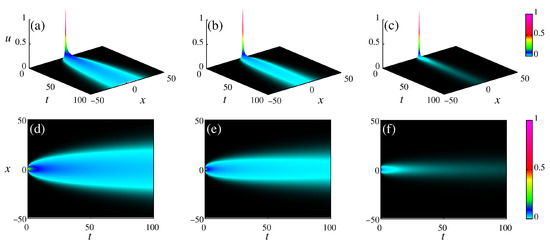
Figure 1. Diffusion of a Gaussian package under time power-law kernel. The panels (a,d) are for $\alpha =0.99$; the panels (b,e) for $\alpha =0.9$; and the panels (c,f) for $\alpha =0.7$. We considered $\Delta t=0.01$, $\Delta x=0.5$, $D=1$, and $\sigma =0.4$.

Figure 2a–c show the profiles in $t=0.02$, 10, 12.5, 25, 50, and 100 by the red, green, black, blue, orange, and dark-green lines, respectively. Figure 2a is for $\alpha =0.99$; Figure 2b is for $\alpha =0.9$; Figure 2c is for $\alpha =0.7$. In the profiles, as time advances, the Gaussian packet is deformed by an anomalous relaxation process, due to the effects of non-integer operators.

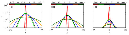
Figure 2. Profiles of Gaussian package. The panels (a–c) are for $\alpha =0.99$, $\alpha =0.9$, and $\alpha =0.7$, respectively. We considered $\Delta t=0.01$, $\Delta x=0.5$, $D=1$, and $\sigma =0.4$.

Figure 3 displays $u(0,t)$ for $\alpha =0.99$, $\alpha =0.90$, and $\alpha =0.70$ by the red, black, and blue lines, respectively. The behavior of $u(0,t)$ is a power-law with slopes equal to 0.5, 0.55, and 0.65 for $\alpha =0.99$, $\alpha =0.90$, and $\alpha =0.70$. As the measured $\alpha$ decreases, the slope associated with $u(0,t)$ increases. The increment is related to the anomalous relaxation process.

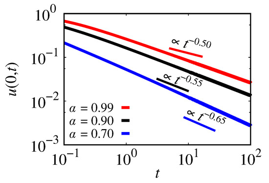
Figure 3. Behavior of $u(0,t)$ as a function of time. The red line is for $\alpha =0.99$; the black line is for $\alpha =0.90$; the blue line is for $\alpha =0.7$. We considered $\Delta t=0.01$, $\Delta x=0.5$, $D=1$, and $\sigma =0.4$.

3.2. Power-Law in Space

Considering the power-law operator (Equation (31)) only in the space derivative, Equation (1) becomes

$$\frac{\partial }{\partial t}u(x,t)=D\frac{{\partial }^{\mu }}{\partial x^{\mu }}u(x,t)+F(x,t),$$

(39)

with ${\Lambda }_{\mu }\left(x\right)$=$x^{1-\mu }/\Gamma (2-\mu )$.

From Equation (15), a numerical expression for Equation (39) is given by

$$\begin{array}{ccc}\hfill u_{i,j+1}& =& u_{i,j}+\frac{D}{\Gamma (3-\mu )}\frac{\Delta t}{\Delta x^{\mu }}\sum _{n=0}^{i-1}(u_{i-n+1,j}-2u_{i-n,j}+u_{i-n-1,j})[{(n+1)}^{2-\mu }-n^{2-\mu }]\hfill \\ & +& \Delta tF(x_i,t_j).\hfill \end{array}$$

(40)

The diffusion of a Gaussian packet under space fractional operators is displayed in Figure 4. Figure 4a–c show the numerical solution for $\mu =1.99$, $\mu =1.7$, and $\mu =1.5$, followed by the respective density plots in Figure 4d–f. The packet advances in time with the same velocity at all times. However, the spread in the space region occurs in a wider behavior. The effects of fractional space derivatives are not as evident as the effects produced by time operators. This occurs due to the multiplicative terms in each contribution in the distinguished numerical schemes.

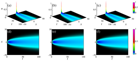
Figure 4. Diffusion of a Gaussian package under power-law space derivative. The panels (a,d) are for $\mu =1.99$; the panels (b,e) for $\mu =1.7$; and the panels (c,f) for $\mu =1.5$. We considered $\Delta t=0.01$, $\Delta x=0.8$, $D=1$, and $\sigma =0.4$.

Figure 5 shows the profiles for $\mu =1.99$ (Figure 5a), $\mu =1.7$ (Figure 5b), and $\mu =1.5$ (Figure 5c) in $t=$ 0.02 (red line), 10 (green line), 12.5 (black line), 25 (blue line), 50 (orange line), and 100 (dark-green line). We verified that the numerical solutions are very similar. This effect can be investigated by looking at the profiles.

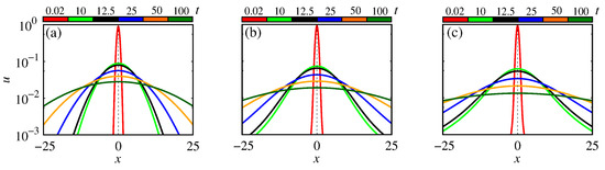
Figure 5. Profiles of Gaussian package for power-law space kernel. The panels (a–c) are for $\mu =1.99$, $\mu =1.7$, and $\mu =1.5$, respectively. We considered $\Delta t=0.01$, $\Delta x=0.8$, $D=1$, and $\sigma =0.4$.

The behavior of $u(0,t)$ as a time function is shown in Figure 6, where the red line is for $\mu =1.99$, the black line for $\mu =1.7$, and the blue line for $\mu =1.5$. The slopes associated with $\mu =1.99$, $\mu =1.7$, and $\mu =1.5$ are 0.49, 0.58, and 0.67, respectively. The slopes oscillate around $0.5$, which is associated with the normal diffusion.

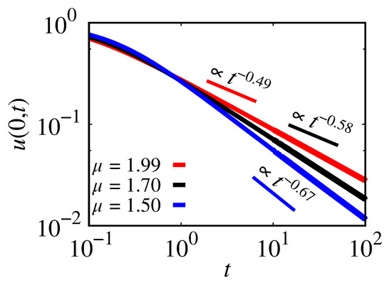
Figure 6. $u(0,t)$ as a function of the time for the power-law space kernel. The red line is for $\mu =1.99$; the black line is for $\mu =1.7$; the blue line is for $\mu =1.5$. We considered $\Delta t=0.01$, $\Delta x=0.8$, $D=1$, and $\sigma =0.4$.

3.3. Power-Law in Time and Space

For the last case, we considered both non-integer operators in the diffusion equation, which is

$$\frac{{\partial }^{\alpha }}{\partial t^{\alpha }}u(x,t)=D\frac{{\partial }^{\mu }}{\partial x^{\mu }}u(x,t)+F(x,t).$$

(41)

For this case, we have ${\mathcal{K}}_{\alpha }\left(t\right)$=$t^{-\alpha }/\Gamma (1-\alpha )$ and ${\Lambda }_{\mu }\left(x\right)$=$x^{1-\mu }/\Gamma (2-\mu )$. Substituting these values in Equation (15) and performing some operations, we obtain

$$\begin{array}{ccc}\hfill u_{i,j+1}& =& u_{i,j}-\sum _{k=1}^j(u_{i,j+1-k}-u_{i,j-k})\left[{(k+1)}^{1-\alpha }-k^{1-\alpha }\right]+\hfill \\ & +& D\frac{\Gamma (2-\alpha )}{\Gamma (3-\mu )}\frac{\Delta t^{\alpha }}{\Delta x^{\mu }}\sum _{n=0}^{i-1}[u_{i-n+1,j}-2u_{i-n,j}+u_{i-n-1,j}][{(n+1)}^{2-\mu }-n^{2-\mu }]\hfill \\ & +& \Delta t^{\alpha }\Gamma (2-\alpha )F(x_i,t_j).\hfill \end{array}$$

(42)

Equation (42) provides a numerical solution for the diffusion equation (Equation (1)), when the power-law kernels in space and time are considered.

Figure 7 displays the diffusion of a Gaussian package with the initial condition equal to $u(x,0)=e^{-x^2/\left(2{\sigma }^2\right)}/\sqrt{2\pi {\sigma }^2}$. Figure 7a–c exhibit the solutions in the three-dimensional space, while Figure 7d–f show the density plot of u (color scale). In these results, we considered $\sigma =0.4$, $\Delta t=0.01$, $\Delta x=0.5$, $D=1$, $\alpha =0.99$, and $\mu =1.99$ in Figure 7a,d, $\alpha =0.9$ and $\mu =1.7$ in Figure 7b,e, and $\alpha =0.7$ and $\mu =1.5$ in Figure 7c,f. These results show that the time fractional operator effects are more prominent than the effects of the space fractional operator. This occurs due to each contribution’s multiplicative terms appearing in Equation (42).

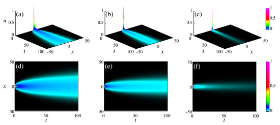
Figure 7. Diffusion of a Gaussian package under time and space power-law kernels. The panels (a,d) are for $\alpha =0.99$ and $\mu =1.99$; panels (b,e) for $\alpha =0.9$ and $\mu =1.7$; and panels (c,f) for $\alpha =0.7$ and $\mu =1.5$. We considered $\sigma =0.4$, $\Delta t=0.01$, $\Delta x=0.75$, and $D=1$.

Figure 8a–c show the profiles for $t=0.02$ (red line), 10 (green line), 12.5 (black line), 25 (blue line), 50 (orange line), and 100 (dark-green line). The panel (a) is for $\alpha =0.99$ and $\mu =1.99$, the panel (b) for $\alpha =0.9$ and $\mu =1.7$, and the panel (c) for $\alpha =0.7$ and $\mu =1.5$. The profiles display that the package spreads slowly in an abnormal process when the fractal orders decrease.

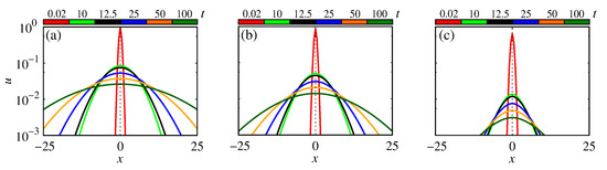
Figure 8. Profiles of Gaussian package for time and space power-law kernels. The panel (a) is for $\alpha =0.99$ and $\mu =1.99$; the panel (b) is for $\alpha =0.9$ and $\mu =1.7$; the panel (c) is for $\alpha =0.7$ and $1.5$. We considered $\sigma =0.4$, $\Delta t=0.01$, $\Delta x=0.75$, and $D=1$.

In the last analysis, we display $u(0,t)$ as a function of time in Figure 9 by the red, black, and blue lines, for $\alpha =0.99$ and $\mu =1.99$, for $\alpha =0.9$ and $\mu =1.7$, and for $\alpha =0.7$ and $\mu =1.5$. As the fractional order decreases, the inclination of each curve decreases. Our results show that the slopes associated with the red, black, and blue curves are given by 0.50, 0.62, and 0.77, respectively. These slopes show that the relaxation process is anomalous and depends on the fractional order. We mixed both effects by combining $\alpha$ and $\mu$.

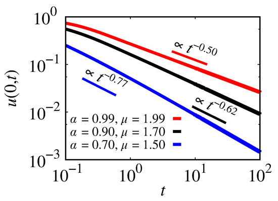
Figure 9. $u(0,t)$ as a function of the time and space power-law kernels. The red line is for $\alpha =0.99$ and $\mu =1.99$. The black line is for $\alpha =0.9$ and $\mu =1.7$. The blue line is for $\alpha =0.7$ and $\mu =1.5$. We considered $\sigma =0.4$, $\Delta t=0.01$, $\Delta x=0.75$, and $D=1$.

4. Fractional Operators—Exponential Kernel

In our second example, we considered the exponential kernel, defined by

$$\begin{array}{c}\hfill {\mathcal{K}}_{\alpha }\left(t\right)=\mathrm{M}\left(\alpha \right)e^{-\frac{\alpha t}{1-\alpha }}/\left(1-\alpha \right),\end{array}$$

(43)

and

$$\begin{array}{c}\hfill {\Lambda }_{\mu }\left(x\right)=\delta \left(x\right),\end{array}$$

(44)

where $\mathrm{M}\left(\alpha \right)$ is the normalization constant. The kernel defined by Equation (44) returns the standard space differential operator. By considering these choices for the kernel, the diffusion equation can be written as follows:

$$\frac{{\partial }^{\alpha }}{\partial t^{\alpha }}u(x,t)=D\frac{{\partial }^2}{\partial x^2}u(x,t)+F(x,t).$$

(45)

The analytical solution for this equation can be found by using the integral transforms, i.e., the Laplace and Fourier transforms [1], which allow us to obtain

$$\begin{array}{c}\hfill u(x,t)={\int }_{-\infty }^{\infty }d{x}^{\prime }{\mathcal{G}}_{\alpha ,1}(x-x^{\prime },t)\overline{u}\left(x\right)+{\int }_{-\infty }^{\infty }d{x}^{\prime }{\int }_0^{t}d{t}^{\prime }{\mathcal{G}}_{\alpha ,2}(x-x^{\prime },t-t^{\prime })F(x^{\prime },t^{\prime }),\end{array}$$

(46)

with

$$\begin{array}{c}\hfill {\mathcal{G}}_{\alpha ,1}(x,t)=\frac{1}{2\pi }{\int }_{-\infty }^{\infty }dk{e}^{ikx}\frac{e^{-\frac{\alpha D{k}^{2}t}{1+(1-\alpha )D{k}^{2}t}}}{1+(1-\alpha )D{k}^2},\end{array}$$

(47)

and

$$\begin{array}{c}\hfill {\mathcal{G}}_{\alpha ,2}(x,t)=\frac{1}{2\pi }{\int }_{-\infty }^{\infty }dk{e}^{ikx}\frac{e^{-\frac{\alpha D{k}^{2}t}{1+(1-\alpha )D{k}^{2}t}}}{{\left[1+(1-\alpha )D{k}^2\right]}^2}+\frac{e^{-\frac{\left|x\right|}{2\sqrt{(1-\alpha )D}}}}{\sqrt{(1-\alpha )D}}\delta \left(t\right).\end{array}$$

(48)

Considering Equation (43), the discretized diffusion equation becomes

$$\begin{array}{ccc}\hfill u_{i,j+1}& =& u_{i,j}-\frac{1}{1-e^{\frac{-\alpha \Delta t}{1-\alpha }}}\sum _{k=1}^j(u_{i,j+1-k}-u_{i,j-k})\left[e^{\frac{-\alpha \Delta t}{1-\alpha }k}-e^{\frac{-\alpha \Delta t}{1-\alpha }(1+k)}\right]\hfill \\ & +& \frac{\alpha D\Delta t}{\mathrm{M}\left(\alpha \right)\Delta x^2\left(1-e^{\frac{-\alpha \Delta t}{1-\alpha }}\right)}(u_{i+1,j}-2u_{i,j}+u_{i-1,j})+\frac{\alpha \Delta tF(x_i,t_j)}{\mathrm{M}\left(\alpha \right)\left(1-e^{\frac{-\alpha \Delta t}{1-\alpha }}\right)};\hfill \end{array}$$

(49)

for simplicity, we considered $\mathrm{M}\left(\alpha \right)=1$ and $F(x_i,t_j)=0$. Equation (49) is a discretization for a non-singular kernel, while Equation (38) is for a singular kernel. When the time operator is discretized for our kernel choices, the terms related to the memory effects decay following a power-law and an exponential function for singular and non-singular kernels. In addition, memory terms are divided by $1-e^{-\alpha \Delta t/(1-\alpha )}$ for the exponential kernel. Due to the product of the operator discretization, multiplicative terms appear in the space derivative and source term. For the singular kernel, memory terms are proportional to $\Delta t^{\alpha }$, while for the non-singular kernel, they are proportional to $\alpha /\left[M\left(\alpha \right)(1-e^{-\alpha \Delta t/1-\alpha })\right]$. These constants carry information about the kernel type.

Numerical solutions for Equation (49) are displayed in Figure 10, where we considered $u(x,0)=e^{-x^2/\left(2{\sigma }^2\right)}/\sqrt{2\pi {\sigma }^2}$, $\sigma =0.4$, $\Delta t=0.01$, $\Delta x=0.5$, $D=1$, and $\mathrm{M}\left(\alpha \right)=1$. Figure 10a,d are for $\alpha =0.99$, Figure 10b,e are for $\alpha =0.97$, Figure 10c,f are for $\alpha =0.95$. The effects of the diffusion process become anomalous. However, the abnormality is not too pronounced. The effects of decreasing $\alpha$ maintain the slope near 0.5.

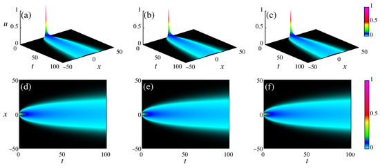
Figure 10. Diffusion of a Gaussian package under exponential kernel. The panel (a,d) is for $\alpha =0.99$; the panel (b,e) is for $\alpha =0.97$; the panel (c,f) is for $\alpha =0.95$. We considered $\sigma =0.4$, $\Delta t=0.01$, $\Delta x=0.5$, $D=1$, and $\mathrm{M}\left(\alpha \right)=1$.

Profiles for $t=0.02$ (red line), 1 (green line), 1.25 (black line), 2.5 (blue line), 5 (orange line), and 10 (dark-green line) are displayed in Figure 11. Figure 11a is for $\alpha =0.99$; Figure 11b is for $\alpha =0.97$; Figure 11c is for $\alpha =0.95$. As observed in the projection shown in Figure 10, the exponential kernel does not affect the dynamics in a pronounced way.

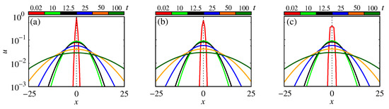
Figure 11. Profiles of Gaussian package for time exponential kernel. The panel (a) is for $\alpha =0.99$; (b) is for $\alpha =0.97$; (c) is for $\alpha =0.95$. We considered $\sigma =0.4$, $\Delta t=0.001$, $\Delta x=0.5$, $D=1$, and $M\left(\alpha \right)=1$.

To validate our algorithm, we compared the numerical solution with the analytical one given by Equation (46). We calculated the relative error by $\Delta E=|u_{\mathrm{sim}}(0,t)-u_{\mathrm{ana}}(0,t)|$. The error is displayed in Figure 12 by the red points for $\alpha =0.99$, black points for $\alpha =0.97$, and blue for $\alpha =0.95$ as a function of time. The error decreases as time advances. Also, the error for $\alpha =0.95$ is greater than the errors for the other two cases. This occurs due to the terms being inversely proportional to the exponential of $\alpha$. We verified that the error can be reduced by decreasing $\Delta x$ and $\Delta t$.

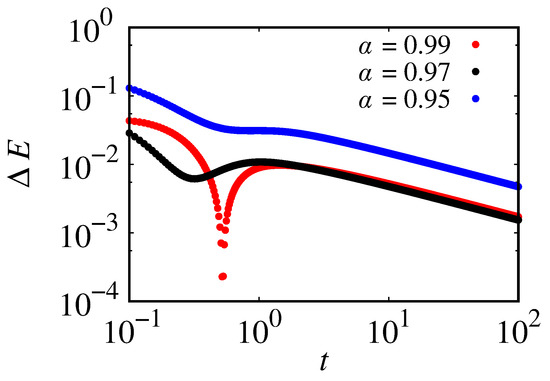
Figure 12. Error among simulated points and analytical ones defined by $\Delta E=|u_{\mathrm{sim}}(0,t)-u_{\mathrm{ana}}(0,t)|$. We considered $\sigma =0.4$, $\Delta t=0.01$, $\Delta x=0.5$, $D=1$, and $M\left(\alpha \right)=1$.

Figure 13 exhibits $u(0,t)$ as a time function for $\alpha =0.99$ (red line), $\alpha =0.97$ (black line), and $\alpha =0.95$ (blue line). In the range $t\in [{10}^{-1},{10}^1]$, the slopes associated with each curve are 0.50, 0.49, and 0.49. Each slope is practically 0.5, indicating a normal diffusion process.

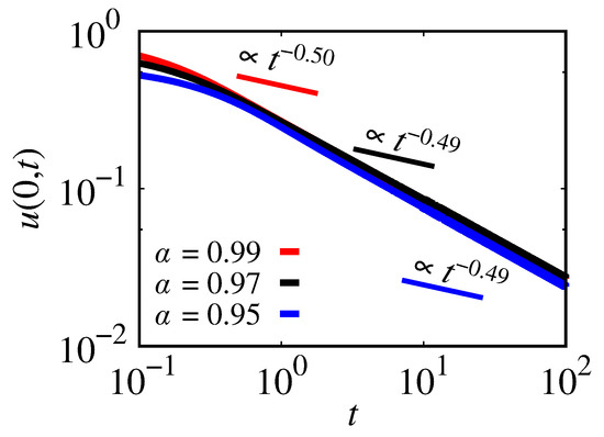
Figure 13. $u(0,t)$ as a function of the time exponential kernel. The red line is for $\alpha =0.99$; the black line is for $\alpha =0.97$; the blue line is for $\alpha =0.95$. We considered $\sigma =0.4$, $\Delta t=0.01$, $\Delta x=0.5$, $D=1$, and $M\left(\alpha \right)=1$.

5. Conclusions

We analyzed a reaction–diffusion equation governed by general fractional operators from the numerical point of view. Considering the finite difference scheme, we proposed a discretization for the fractional reaction–diffusion equation under the general kernel, acting in space and time. In addition, we investigated and obtained the stability conditions that explicitly depend on the kernel type. As a numerical application, we considered two distinct kernels: power-law and exponential. For the power-law kernel, we studied the effects when the fractional operator acts in time, space, and both derivatives. On the other hand, for the exponential kernel, we investigated their action only in the time derivative. For this case, we compared the simulation with our analytical solution. The results showed an error of less than ${10}^{-1}$.

One limitation of the method is the entire dependence of the results from the integrals that appear in Equation (15), which can be hard to calculate in some cases. Another challenge is the numerical implementation. In this work, we presented two numerical examples. Due to the stability conditions, the implementation of an exponential kernel spends more computational cost than a power-law kernel. In addition, for another kernel choice, it is important to consider an adequate grid size, which is a determinant factor in the solution convergence. Our results showed that our algorithm works for different kernel choices and can also be used to investigate anomalous diffusion, which agrees with analytical solutions for specific cases. Other works proposed discrete forms for general time kernel [54,55]. In a particular case, the diffusion equation under the space general kernel was also explored in [56], where the authors obtained analytical solutions. Our results are in agreement with these works. The novelty of our work is based on the investigation of numerical solutions, as well as their stability for general kernels acting in both operators.

In summary, the fractal derivatives can be considered to explore aspects in which the usual operators are not suitable to capture the system’s behavior, such as memory effects and long-range correlations. When power-law kernels are considered, these effects have implications in the relaxation process, which is related to the solutions proportionally with Mittag–Leffler functions, which are asymptotically governed by power-laws. Specifically, our results showed that the numerical procedure developed in this work can be employed to solve fractional differential equations considering different kernels. Our methodology can be extended to study high-order problems, as studied by Zhang et al. [57], which are topics for future works.

References

- Evangelista, L.R.; Lenzi, E.K. Fractional Diffusion Equations and Anomalous Diffusion; Cambridge University Press: Cambridge, UK, 2018. [Google Scholar]
- Paul, A.; Laurila, T.; Vuorinen, V.; Divinski, S.V. Thermodynamics, Diffusion and the Kirkendall Effect in Solids; Springer: Cham, Switzerland, 2014. [Google Scholar]
- Da Silva, S.T.; Viana, R.L. Reaction-diffusion equation with stationary wave perturbation in weakly ionized plasmas. Braz. J. Phys. 2020, 50, 780–787. [Google Scholar] [CrossRef]
- Benetti, M.H.; Silveira, F.E.M.; Caldas, I.L. Fundamental solution of diffusion equation for Kappa gas: Diffusion length for suprathermal electrons in solar wind. Phys. Rev. E 2023, 107, 055212. [Google Scholar] [CrossRef] [PubMed]
- Salman, A.M.; Mohd, M.H.; Muhammad, A. A novel approach to investigate the stability analysis and the dynamics of reaction–diffusion SVIR epidemic model. Commun. Nonlinear Sci. Numer. Simul. 2023, 126, 107517. [Google Scholar] [CrossRef]
- Zhao, H.; Zhu, L. Dynamic Analysis of a Reaction–DiffusionRumor Propagation Model. Int. J. Bifurc. Chaos 2016, 26, 1650101. [Google Scholar] [CrossRef]
- Pinar, Z. An Analytical Studies of the Reaction-Diffusion Systems of Chemical Reactions. Int. J. Appl. Comput. Math. 2021, 7, 81. [Google Scholar] [CrossRef]
- Ganguly, S.; Neogi, U.; Chakrabarti, A.S.; Chakraborti, A. Reaction-diffusion equations with applications to economic systems. In Proceedings of the Econophysics and Sociophysics: Recent Progress and Future Directions; Springer: Cham, Switzerland, 2017; pp. 131–144. [Google Scholar]
- Essa, K.; Etman, S.M.; El-Otaify, M.S.; Embaby, M.; Mosallem, A.M.; Shalaby, A.S. Different solutions of the diffusion equation and its applications. J. Basic Appl. Sci. 2021, 10, 82. [Google Scholar] [CrossRef]
- Leonel, E.D.; Kuwana, C.M.; Yoshida, M.; Oliveira, J.A. Application of the diffusion equation to prove scaling invariance on the transition from limited to unlimited diffusion. Europhys. Lett. 2020, 131, 10004. [Google Scholar] [CrossRef]
- Lenzi, E.; Lenzi, M.; Ribeiro, H.; Evangelista, L. Extensions and solutions for non-linear diffusion equations and random walks. Proc. R. Soc. A 2019, 475, 20190432. [Google Scholar] [CrossRef]
- Belova, I.V.; Afikuzzaman, M.; Murch, G.E. A new approach for analysing interdiffusion in multicomponent alloys. Scr. Mater. 2021, 204, 114143. [Google Scholar] [CrossRef]
- Belova, I.V.; Afikuzzaman, M.; Murch, G.E. Novel Interdiffusion Analysis in Multicomponent Alloys—Part 2: Application to Quaternary, Quinary and Higher Alloys. Diffus. Found. 2021, 29, 179–203. [Google Scholar] [CrossRef]
- Luo, H.; Liu, W.; Gong, H.; Liang, C. First Principles Calculation of Composition Dependence Tracer and Interdiffusion with Phase Change: A Case Study of Ir/Ir3nb Superalloy. SSRN 2023. [Google Scholar] [CrossRef]
- Li, F.; Feng, J.; Zhang, H.; Li, W.Y. Particle-scale heat and mass transfer processes during the pyrolysis of millimeter-sized lignite particles with solid heat carriers. Appl. Therm. Eng. 2023, 219, 119372. [Google Scholar] [CrossRef]
- Markowich, P.A.; Szmolyan, P. A system of convection–diffusion equations with small diffusion coefficient arising in semiconductor physics. J. Differ. Eqs. 1989, 81, 234–254. [Google Scholar] [CrossRef][Green Version]
- Chaffey, N. Molecular Biology of the Cell; Oxford University Press: Oxford, UK, 2003. [Google Scholar]
- Kucharski, A.J.; Russell, T.W.; Diamond, C.; Liu, Y.; Edmunds, J.; Funk, S.; Eggo, R.M. Early dynamics of transmission and control of COVID-19: A mathematical modelling study. Lancet Infect. Dis. 2020, 20, 553–558. [Google Scholar] [CrossRef] [PubMed]
- Ratnakar, R.R.; Dindoruk, B. The Role of Diffusivity in Oil and Gas Industries: Fundamentals, Measurement, and Correlative Techniques. Processes 2022, 10, 1194. [Google Scholar] [CrossRef]
- Criado, C.; Galán-Montenegro, P.; Velásquez, P.; Ramos-Barrado, J. Diffusion with general boundary conditions in electrochemical systems. J. Electroanal. Chem. 2000, 488, 59–63. [Google Scholar] [CrossRef]
- Yan, H.S.; Ma, K.P. Competitive diffusion process of repurchased products in knowledgeable manufacturing. Eur. J. Oper. Res. 2011, 208, 243–252. [Google Scholar] [CrossRef]
- Mahajan, V.; Muller, E.; Bass, F.M. New product diffusion models in marketing: A review and directions for research. J. Mark. 1990, 54, 1–26. [Google Scholar] [CrossRef]
- Shinde, A.; Takale, K. Study of Black–Scholes Model and its Applications. Procedia Eng. 2012, 38, 270–279. [Google Scholar] [CrossRef]
- Lebedeva, M.I.; Brantley, S.L. Weathering and erosion of fractured bedrock systems. Earth Surf. Process. Landforms 2017, 42, 2090–2108. [Google Scholar] [CrossRef]
- Pant, P. Diffusion Equations for Fluid Flow in Porous Rocks. SAMRIDDHI J. Phys. Sci. Eng. Technol. 2017, 9, 5–13. [Google Scholar] [CrossRef]
- Watson, E.B.; Baker, D.R. Chemical diffusion in magmas: An overview of experimental results and geochemical applications. In Physical Chemistry of Magmas; Springer: New York, NY, USA, 1991; pp. 120–151. [Google Scholar]
- Crank, J. The Mathematics of Diffusion; Oxford University Press: Oxford, UK, 1975. [Google Scholar]
- Almeida, R.; Bastos, N.R.; Monteiro, M.T.T. Modeling some real phenomena by fractional differential equations. Math. Methods Appl. Sci. 2016, 39, 4846–4855. [Google Scholar] [CrossRef]
- Tarasov, V.; Zaslavsky, G. Fractional dynamics of systems with long-range interaction. Commun. Nonlinear Sci. Numer. Simul. 2011, 11, 885–898. [Google Scholar] [CrossRef]
- Al-Refai, M.; Abdeljawad, T. Analysis of the fractional diffusion equations with fractional derivative of non-singular kernel. Adv. Differ. Eqs. 2017, 2017, 315. [Google Scholar] [CrossRef]
- Luchko, Y. Fractional differential equations with the general fractional derivatives of arbitrary order in the Riemann–Liouville sense. Mathematics 2022, 10, 849. [Google Scholar] [CrossRef]
- Almeida, R.; Malinowska, A.B.; Monteiro, M.T.T. Fractional differential equations with a Caputo derivative with respect to a kernel function and their applications. Math. Methods Appl. Sci. 2018, 41, 336–352. [Google Scholar] [CrossRef]
- Hassan, S.K.; Alazzawi, S.N.A.; Ibrahem, N.M. Some Results in Grűnwald–Letnikov Fractional Derivative and its Best Approximation. J. Phys. Conf. Ser. 2021, 1818, 012020. [Google Scholar] [CrossRef]
- Odibat, Z.; Baleanu, D. On a New Modification of the Erdélyi–Kober Fractional Derivative. Fractal Fract. 2021, 5, 121. [Google Scholar] [CrossRef]
- Omaba, M.E.; Enyi, C.D. Atangana–Baleanu time-fractional stochastic integro-differential equation. Partial. Differ. Equ. Appl. Math. 2021, 4, 100100. [Google Scholar] [CrossRef]
- Herrmann, R. Fractional Calculus: An Introduction for Physicists; World Scientific: Singapore, 2014. [Google Scholar]
- Guo, B.; Pu, X.; Huang, F. Fractional Partial Differential Equations and Their Numerical Solutions; World Scientific: Singapore, 2015. [Google Scholar]
- Lin, Y.; Xu, C. Finite difference/spectral approximations for the time-fractional diffusion equation. J. Comput. Phys. 2007, 225, 1533–1552. [Google Scholar] [CrossRef]
- Li, L.; Wang, D. Numerical stability of Grünwald–Letnikov method for time fractional delay differential equations. BIT Numer. Math. 2022, 62, 995–1027. [Google Scholar] [CrossRef]
- Tian, Q.; Yang, X.; Zhang, H.; Xu, D. An implicit robust numerical scheme with graded meshes for the modified Burgers model with nonlocal dynamic properties. Comput. Appl. Math. 2023, 42, 1–26. [Google Scholar] [CrossRef]
- Jiang, X.; Wang, J.; Wang, W.; Zhang, H. A Predictor–Corrector Compact Difference Scheme for a Nonlinear Fractional Differential Equation. Fractal Fract. 2023, 7, 521. [Google Scholar] [CrossRef]
- Yang, X.; Wu, L.; Zhang, H. A space-time spectral order sinc-collocation method for the fourth-order nonlocal heat model arising in viscoelasticity. Appl. Math. Comput. 2023, 457, 128192. [Google Scholar] [CrossRef]
- Zhang, H.; Yang, X.; Tang, Q.; Xu, D. A robust error analysis of the OSC method for a multi-term fourth-order sub-diffusion equation. Comput. Math. Appl. 2022, 109, 180–190. [Google Scholar] [CrossRef]
- Zayernouri, M.; Matzavinos, A. Fractional Adams–Bashforth/Moulton methods: An application to the fractional Keller–Segel chemotaxis system. J. Comput. Phys. 2016, 317, 1–14. [Google Scholar] [CrossRef]
- Li, C.; Zeng, F. Finite difference methods for fractional differential equations. Int. J. Bifurc. Chaos 2012, 22, 1230014. [Google Scholar] [CrossRef]
- Daftardar-Gejji, V.; Sukale, Y.; Bhalekar, S. A new predictor–corrector method for fractional differential equations. Appl. Math. Comput. 2014, 244, 158–182. [Google Scholar] [CrossRef]
- Shen, S.; Liu, F. Error analysis of an explicit finite difference approximation for the space fractional diffusion equation with insulated ends. Anziam J. 2005, 46, C871–C887. [Google Scholar] [CrossRef]
- Liu, F.; Shen, S.; Anh, V.; Turner, I.T. Analysis of a discrete non-Markovian random walk approximation for the time fractional diffusion equation. Anziam J. 2005, 46, C488–C504. [Google Scholar] [CrossRef]
- Yang, Q.; Liu, F.; Turner, I. Numerical methods for fractional partial differential equations with Riesz space fractional derivatives. Appl. Math. Model. 2010, 34, 200–218. [Google Scholar] [CrossRef]
- Chan, T.F. Stability Analysis of Finite Difference Schemes for the Advection-Diffusion Equation. SIAM J. Numer. Anal. 1984, 21, 272–284. [Google Scholar] [CrossRef]
- Konangi, S.; Palakurthi, N.K.; Ghia, U. von Neumann stability analysis of first-order accurate discretization schemes for one-dimensional (1D) and two-dimensional (2D) fluid flow equations. Comput. Math. Appl. 2018, 75, 643–665. [Google Scholar] [CrossRef]
- Evangelista, L.R.; Lenzi, E.K. An Introduction to Anomalous Diffusion and Relaxation; Springer Nature: Cham, Switzerland, 2023. [Google Scholar]
- Mathai, A.M.; Saxena, R.K.; Haubold, H.J. The H-Function; Springer: New York, NY, USA, 2010. [Google Scholar]
- Fan, E.; Li, C.; Stynes, M. Discretised general fractional derivative. Math. Comput. Simul. 2023, 208, 501–534. [Google Scholar] [CrossRef]
- Zhao, D.; Luo, M. Representations of acting processes and memory effects: General fractional derivative and its application to theory of heat conduction with finite wave speeds. Appl. Math. Comput. 2019, 346, 531–544. [Google Scholar] [CrossRef]
- Malacarne, L.C.; Mendes, R.S.; Lenzi, E.K.; Lenzi, M.K. General solution of the diffusion equation with a nonlocal diffusive term and a linear force term. Phys. Rev. E 2006, 74, 042101. [Google Scholar] [CrossRef] [PubMed]
- Zhang, H.; Liu, Y.; Yang, X. An efficient ADI difference scheme for the nonlocal evolution problem in three-dimensional space. J. Appl. Math. Comput. 2023, 69, 651–674. [Google Scholar] [CrossRef]
Disclaimer/Publisher’s Note: The statements, opinions and data contained in all publications are solely those of the individual author(s) and contributor(s) and not of MDPI and/or the editor(s). MDPI and/or the editor(s) disclaim responsibility for any injury to people or property resulting from any ideas, methods, instructions or products referred to in the content. |
© 2023 by the authors. Licensee MDPI, Basel, Switzerland. This article is an open access article distributed under the terms and conditions of the Creative Commons Attribution (CC BY) license (https://creativecommons.org/licenses/by/4.0/).