Disturbance Observer-Based Event-Triggered Adaptive Command Filtered Backstepping Control for Fractional-Order Nonlinear Systems and Its Application

Abstract

This paper considers the disturbance observer-based event-triggered adaptive fuzzy tracking control issue for a class of fractional-order nonlinear systems (FONSs) with quantized signals and unknown disturbances. To improve the disturbance rejection ability, a fractional-order nonlinear disturbance observer (FONDO) is designed to estimate the unknown composite disturbances. Furthermore, by combining an improved fractional-order command-filtered backstepping control technique and an event-triggered control mechanism, an event-triggered adaptive fuzzy quantized control scheme is established, which guarantees the desired tracking performance can be achieved even in the presence of network constraint. Finally, the validity and superiority of the theoretic results are verified by a fractional-order horizontal platform system.

1. Introduction

On account of the notable merits of fractional calculus in modeling and characterizing accurate dynamical properties of many real-world systems, fractional-order systems (FOSs) have received wide attention. Therefore, various control methods were extended to investigate the control problem of FOSs [1,2,3,4,5,6,7,8]. In [5], the necessary and sufficient conditions were proposed to guarantee the stability of a class of fractional-order (FO) descriptor systems. In [8], an adaptive neural control design was developed to guarantee the uniform stability of the closed-loop system (CLS) and avoid the violation of the preassigned state constraints. To handle the mismatched uncertainties effectively, the adaptive backstepping control method was widely utilized to achieve the tracking control of fractional-order nonlinear systems (FONSs) due to its structural design and strong robustness to mismatched uncertainties [9,10,11]. In [10], Liu et al. presented an adaptive fuzzy recursive control algorithm to guarantee the boundedness of the resulting CLS based on direct fractional Lyapunov stability. However, the traditional backstepping design method relies on the repeated differentiation of virtual control laws in the recursive procedure, which undoubtedly will cause the issue of the explosion of complexity and over-parametrization once the dimensionality of the system is overlarge. To overcome this problem, inspired by the integer-order results [12,13,14,15,16], some research works have reported using a modified FODSC technique for FONSs [17,18,19,20,21]. It should be noted that the efforts have barely been made on the composite disturbances consisting of the disturbances and approximation errors in the aforementioned results, where the considered disturbance term is always handled by using the inequality technique or designing a general compensation function. However, it is worth pointing out that the disturbance rejection ability of the existing adaptive control method proposed for the FONSs needs to be further improved to maintain the desired control performance when the investigated system suffers strong changing unknown disturbances.

As we know, unknown disturbances exist in nearly all actual systems; their existence frequently undoubtedly degrades the performance and even destroy the system’s stability. To improve the disturbance rejection ability of the system, the disturbance observer (DO)-based control technique has attracted considerable attention and some significant results have been reported for various types of nonlinear systems [22,23,24,25,26,27,28]. In [23], Chen et al. proposed a DO-based synchronization control method to handle the robust synchronization issue of two FO chaotic systems. In [26], a super twisting nonlinear disturbance observer was designed to guarantee the finite-time convergence of the estimation errors. Nevertheless, it is noted that most of the available DO-based adaptive control results are concentrated on integer-order nonlinear systems. Thus, developing an NDO-based adaptive backstepping control strategy for a class of FONSs remains an open problem.

On the other hand, it is universally known that real-time data are usually quantized in some practical industrial processing control systems due to the influence of bandwidth limitations. Therefore, one major challenge is how to realize the predefined control goal of the CLSs by the quantized control signals. To this end, substantial attention has been paid to adaptive backstepping quantized control for nonlinear systems [29,30,31,32]. In [30], Liu et al. proposed a novel fuzzy quantized recursive control scheme for nonlinear systems. In [32], Sui et al. proposed a finite-time quantized control method for stochastic nonlinear systems, where the traditional power form was not required for determining the control signals. Another effective way of reducing the communication burden is the even-triggered control method. In recent years, a series of event-triggered mechanisms have been developed for nonlinear systems [33,34]. In [33], three different kinds of event-triggered mechanisms were developed to co-design adaptive controllers, which have been widely utilized to address the event-triggered adaptive control problem. Unfortunately, the available adaptive backstepping control methods for FONSs were concentrated on the time-triggered control scheme, as in [17,19,20], where a large number of network communication resources were required since the control signals need to be updated periodically. Therefore, the event-triggered control problem for FONSs needs to be further investigated. Furthermore, a new challenge arises that the complexity of controller design has to be faced when input quantization and the event-triggered control are considered simultaneously. Therefore, how to develop a suitable event-triggered adaptive quantized controller for FONSs also motivates this work.

Inspired by the above observation, we aim to develop a novel FONDO-based event-triggered adaptive fuzzy tracking control method for the FONSs with input quantization in this paper. In comparison with other relevant studies, the main contributions of this paper are as follows:

(1) To the best of our knowledge, this paper first attempts to develop a FONDO-based event-triggered adaptive fuzzy tracking control scheme for unknown FONSs. Compared with the existing adaptive backstepping control results [3,10,11,17,18,19,20], the disturbance rejection ability against the mismatched disturbance can be greatly improved by the proposed FONDO.

(2) A co-design consisting of the event-triggered communication mechanism and input quantization is established such that a large amount of communication resources can be saved while fulfilling the preassigned tracking task in comparison to the traditional time-triggered control methods proposed in [3,10,11,17,18,19,20].

(3) Distinct from the logarithmic quantizer in [35,36] and hysteretic quantizer in [29,31], an adjustable parameter is introduced to the quantizer for achieving the trade-off between the quantization effects and control performance. Also, the saturation property is adopted to keep the control energy within bounds, making the proposed control method closer to the practical requirements.

The remaining part of this paper consists of the following sections. Section 2 presents the preliminaries and formulates the considered problem. A disturbance observer-based event-triggered adaptive quantized control method is developed for a class of unknown fractional-order nonlinear systems in Section 3. Section 4 provides an application example to verify the feasibility and superiority of the developed method. Finally, the whole work and the potential improvements are concluded in Section 5.

2. Preliminaries and Problem Formulation

2.1. Fractional Calculus

Definition 1

([37]). The Caputo fractional derivative of order α of a function $f\left(t\right)$ is

$$D^{\alpha }f\left(t\right)=\frac{1}{\Gamma (n-\alpha )}{\int }_0^t\frac{f^{\left(n\right)}\left(\tau \right)}{{(t-\tau )}^{\alpha +1-n}}d\tau$$

(1)

where $n-1<\alpha \le n$.

Definition 2

([37]). The Mittag-Leffler function including two parameters is expressed as:

$$E_{{\alpha }_1,{\alpha }_2}\left(r\right)=\underset{i=0}{\sum ^{\infty }}\frac{r^i}{\Gamma (i{\alpha }_1+{\alpha }_2)},$$

(2)

where ${\alpha }_1>0$, ${\alpha }_2>0$ and r is a complex number. Taking the Laplace transform (LT) for the above equation, one has

$$\mathcal{L}\left\{t^{{\alpha }_2-1}{E}_{{\alpha }_1,{\alpha }_2}(-\kappa t^{{\alpha }_1})\right\}=\frac{s^{{\alpha }_1-{\alpha }_2}}{s^{{\alpha }_1}+\kappa }.$$

(3)

Lemma 1

([37]). For ${\alpha }_1\in (0,2)$, if there exists a positive constant ℓ such that $\pi {\alpha }_1/2<\ell <min\left\{\pi ,\pi {\alpha }_1\right\}$, then the following inequality holds

$$\left|E_{{\alpha }_1,{\alpha }_2}\left(r\right)\right|\le \frac{\hslash }{1+\left|r\right|},(\ell \le |arg\left(r\right)|\le \pi ,|r|\ge 0),$$

(4)

where ${\beta }_2$ is a real number and $\hslash >0$.

Lemma 2

([37]). For ${\alpha }_1\in (0,2)$, if there exist an arbitrary complex number ${\alpha }_2$ and a real number ℓ such that

$$\frac{\pi {\alpha }_1}{2}<\ell <min(\pi ,\pi {\alpha }_1),$$

(5)

then it can be verified that

$$\begin{array}{cc}\hfill E_{{\alpha }_1,{\alpha }_2}\left(r\right)=& -\underset{i=1}{\sum ^{\infty }}\frac{r^{-i}}{\Gamma ({\alpha }_2-i{\alpha }_1)}+{o\left(\right|r|}^{-1-\ell }),|r|\to \infty ,\ell \le \left|arg\left(r\right)\right|\le \pi \hfill \end{array}$$

(6)

for all integers $\ell \ge 1$.

2.2. Fuzzy Logic Systems

To better achieve the mentioned control objective, fuzzy logic systems (FLSs) are adopted in this paper to handle the unknown nonlinearities. Consider k fuzzy IF–THEN rules with the following form [11]:

$${\mathbb{R}}^s: \mathrm{if} x_1 \mathrm{is} F_1^s \mathrm{and}\dots \mathrm{and} x_n \mathrm{is} F_n^s$$

$$\mathrm{Then} , y \mathrm{is} G^s, s=1,\dots ,k$$

where ${\mathbb{R}}^s$ represents the sth rule, $1\le s\le k,x_i(i=1,\dots ,n)$, and $y\in \mathbb{R}$ denote the linguistic variables associated with the inputs and outputs of the FLSs, respectively. $F_i^s$ and $G^s$ are the fuzzy set. In this article, the FLSs are described as

$$y\left(x\right)=\frac{{\sum }_{s=1}^k{w}_s\left({\prod }_{i=1}^n{\mu }_{F_i^s}\left(x_i\right)\right)}{{\sum }_{s=1}^k\left({\prod }_{i=1}^n{\mu }_{F_i^s}\left(x_i\right)\right)}.$$

(7)

Define the weight vector and fuzzy basis function vector as $W={[w_1,\dots ,w_k]}^T$ and $\varphi \left(x\right)={\left[{▵}_1,\dots ,{▵}_k\right]}^T$, where ${▵}_s=\left[\left({\prod }_{i=1}^n{\mu }_{F_i^s}\left(x_i\right)\right)/{\sum }_{s=1}^k\left({\prod }_{i=1}^n{\mu }_{F_i^s}\left(x_i\right)\right)\right]$; then, the above expression can be represented as

$$y\left(x\right)=W^T\varphi \left(x\right).$$

(8)

Lemma 3

([11]). For any continuous function $f\left(x\right)$ defined over a compact set Θ and any given constant o, there exist an FLS and an ideal weight vector $W^{\ast }$ such that

$$\begin{array}{c}\hfill \underset{x\in \Theta }{sup}|f\left(x\right)-{W^{\ast }}^T\varphi \left(x\right)|\le ϵ.\end{array}$$

(9)

Lemma 4

([38]). For $z\in \mathbb{R}$ and positive constant ϖ, the following inequality holds

$$0\le \left|z\right|-\frac{z^2}{\sqrt{z^2+{\varpi }^2}}<\varpi .$$

(10)

2.3. Problem Formulation

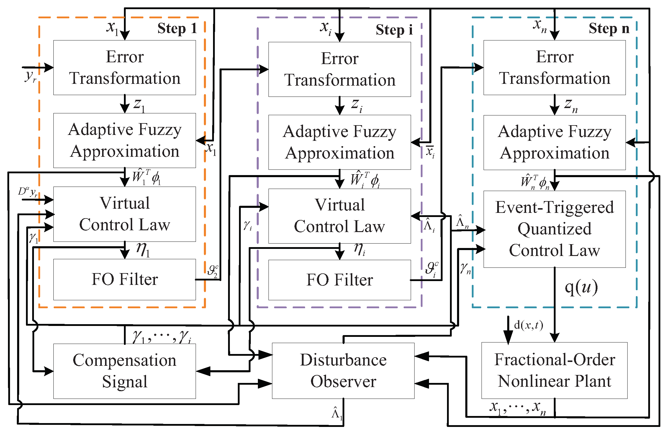
Consider a class of FONSs subject to input quantization and unknown disturbances described by

$$\begin{array}{c}\hfill \left\{\begin{array}{cc}\hfill D^{\alpha }{x}_i=& x_{i+1}+f_i\left({\overline{x}}_i\right)+d_i(x,t),\left(i=1,\dots ,n-1\right),\hfill \\ \hfill D^{\alpha }{x}_n=& q\left(u\right)+f_n\left({\overline{x}}_n\right)+d_n(x,t)\hfill \\ \hfill y=& x_1,\hfill \end{array}\right.\end{array}$$

(11)

where $x={\overline{x}}_n={\left[x_1,\dots ,x_n\right]}^T\in {\mathbb{R}}^n$ is the state vector; $y\in \mathbb{R}$ denotes the system output; $f_i\left({\overline{x}}_i\right)$ represents an unknown but smooth nonlinear function; $d_i(x,t)$ represents the unknown but bounded disturbance terms; and $q\left(u\right)$ represents the quantized control signal. To reduce the chattering phenomenon, the following hysteresis quantizer is considered to obtain a quantized control signal:

$$\begin{array}{c}\hfill q\left(u\right)=\left\{\begin{array}{cc}\hfill & u_i\mathrm{sgn}\left(u\right),\frac{u_i}{1+\delta }<\left|u\right|\le u_i,\dot{u}<0,\mathrm{or}\hfill \\ \hfill & u_i<\left|u\right|\le \frac{u_i}{1-\delta },\dot{u}>0\hfill \\ \hfill & u_i(1+\delta )\mathrm{sgn}\left(u\right),u_i<\left|u\right|\le \frac{u_i}{1-\delta },\dot{u}<0,\mathrm{or}\hfill \\ \hfill & \frac{u_i}{1-\delta }<\left|u\right|\le \frac{u_i(1+\delta )}{1-\delta },\dot{u}>0\hfill \\ \hfill & 0,0\le \left|u\right|<\frac{u_{min}}{1+\delta },\dot{u}<0,\mathrm{or}\hfill \\ \hfill & \frac{u_{min}}{1+\delta }\le \left|u\right|\le u_{min},\dot{u}>0\hfill \\ \hfill & q\left(u\left(t^{-}\right)\right),\mathrm{otherwise}\hfill \end{array}\right.\end{array}$$

(12)

where $u_i={\rho }^{1-i}{u}_{min}(i=1,2,\dots )$ with $0<\rho <1$ and $\delta =\frac{1-\rho }{1+\rho }$, $u_{min}$ denotes the scope of the dead-zone for $q\left(u\right)$ and $q\left(u\left(t^{-}\right)\right)$ represents the status prior to $q\left(u\right(t\left)\right)$.

Lemma 5

([30]). The quantizer $q\left(u\right)$ can be expressed as $q\left(u\right)=(1-\kappa )u+\kappa \theta$ with the quantizer error ϖ satisfying

$$\begin{array}{c}\hfill \left\{\begin{array}{cc}\hfill {\theta }^2\le & {\left(\frac{\kappa +\delta }{\kappa }u\right)}^2,\forall u\ge \left|u_{min}\right|,\hfill \\ \hfill {\theta }^2\le & {\left(\frac{1-\kappa }{\kappa }{u}_{min}\right)}^2,\forall u\le \left|u_{min}\right|,\hfill \end{array}\right.\end{array}$$

(13)

where $0<\theta <1$ is a constant.

Remark 1.

The parameter ρ stands for a measure of quantization density. Compared with the logarithmic quantizer, the hysteretic quantizer can reduce the chattering effectively, which can be viewed as a special combination of two asymmetric logarithmic quantizers. In addition, the value of κ, as an adjustable design parameter, could be selected appropriately by the designer to balance the control performance and quantization effects, which also increases the freedom of quantization design.

Assumption 1.

The reference signal $y_r$ and its FO derivative $D^{\alpha }{y}_r$ are available and bounded.

Assumption 2.

For the external disturbance $d_i(x,t)$, there exist the unknown positive constants ${\overline{d}}_{i,1}$ and ${\overline{d}}_{i,2}$ such that the inequalities $|d_i|\le {\overline{d}}_{i,1}$ and $|D^{\alpha }{d}_i|\le {\overline{d}}_{i,2}$ hold.

The control objective of this work is devoted to presenting a nonlinear disturbance observer-based event-triggered adaptive quantized tracking control scheme for system (11) such that all the signals of the CLS are bounded and the tracking error converges to a small neighborhood of the origin.

3. Main Results

In this section, an NDO-based event-triggered adaptive command-filtered quantized control scheme will be developed for system (11) by integrating with the FOCFB technique and ETC mechanism. Then, the stability analysis of the CLS will be presented based on Mittag-Leffler stability.

NDO-Based Event-Triggered Adaptive Command-Filtered Quantized Control Design

Step 1. At first, we introduce the change of coordinates as:

$$\left\{\begin{array}{cc}\hfill z_1& =x_1-y_r,\hfill \\ \hfill z_i& =x_i-{\vartheta }_i^c,(i=2,\dots ,n),\hfill \end{array}\right.$$

(14)

where $z_j(j=1,\dots ,n)$ denotes surface error and ${\vartheta }_i^c$ is an auxiliary variable used for approximating the virtual control signal, which is produced by

$${\iota }_2{D}^{\alpha }{\vartheta }_2^c+{\vartheta }_2^c={\eta }_1,{\vartheta }_2^c\left(0\right)={\eta }_1\left(0\right),$$

(15)

where ${\iota }_2>0$ is a small time constant and ${\eta }_1$ is the input of the FO filter. Define the filter error ${\epsilon }_1={\vartheta }_{2,c}-{\eta }_1$. To reduce the negative effects caused by filter errors, the compensation signal is constructed as:

$$\begin{array}{c}\hfill D^{\alpha }{\gamma }_1=-a_1{\gamma }_1-{\Delta }_1{\gamma }_1+{\epsilon }_1,\end{array}$$

(16)

where ${\Delta }_1=\frac{|z_1{ϵ}_1|}{{\gamma }_1^2}$ and $a_1$ is a positive constant.

According to Lemma 3, the FO derivative of $z_1$ is computed as:

$$\begin{array}{c}\hfill D^{\alpha }{z}_1=z_2+{\eta }_1+{\epsilon }_1+l_1^{-1}{W}_1^{\ast T}{\varphi }_1\left(x_1\right)+{\Lambda }_1-D^{\alpha }{y}_r,\end{array}$$

(17)

where the FLS is used to approximate the term $F_1\left(x_1\right)=l_1{f}_1\left(x_1\right)$ and ${\Lambda }_1=d_1+l_1^{-1}{ϵ}_1$ denotes an unknown composite disturbance satisfying ${\Lambda }_1\le {\overline{d}}_1^1+l_1^{-1}{\overline{ϵ}}_1^1$.

The first virtual control function ${\alpha }_1$ and adaptive law are designed as:

$$\begin{array}{cc}\hfill & {\eta }_1=-\frac{z_1{\overline{\eta }}_1^2}{\sqrt{z_1^2{\overline{\eta }}_1^2+{\varpi }_1^2}},\hfill \end{array}$$

(18)

$$\begin{array}{cc}\hfill & {\overline{\eta }}_1=(c_1+\frac{1+b_1}{2})z_1+l_1^{-1}{\widehat{W}}_1^T{\varphi }_1\left(x_1\right)-b_1{\gamma }_1-D^{\alpha }{y}_r+{\widehat{\Lambda }}_1,\hfill \end{array}$$

(19)

$$\begin{array}{cc}\hfill & D^{\alpha }{\widehat{W}}_1=l_1^{-1}{z}_1{\varphi }_1\left(x_1\right)-{\rho }_1{\widehat{W}}_1,\hfill \end{array}$$

(20)

where $b_1,c_1,{\rho }_1$ and $l_1$ are all positive constants.

Select the Lyapunov function with the following form:

$$V_1=\frac{1}{2}{z}_1^2+\frac{1}{2}{{\tilde{W}}_1}^T{\tilde{W}}_1+\frac{1}{2}{{\gamma }_1}^2+\frac{1}{2}{\tilde{\Lambda }}_1^2$$

(21)

Taking the FO derivative of $V_1$ yields

$$\begin{array}{cc}\hfill D^{\alpha }{V}_1\le & z_1{\eta }_1+z_1\left(z_2+{\epsilon }_1+l_1^{-1}{W}_1^{\ast T}{\varphi }_1\left(x_1\right)+{\Lambda }_1-D^{\alpha }{y}_r\right)\hfill \\ \hfill & -{\tilde{W}}_1^T{D}^{\alpha }{\widehat{W}}_1+{\gamma }_1{D}^{\alpha }{\gamma }_1+{\tilde{\Lambda }}_1{D}^{\alpha }{\tilde{\Lambda }}_1.\hfill \end{array}$$

(22)

Subsequently, the following FONDO is designed to obtain the estimation of the composite disturbance ${\Lambda }_1$

$${\widehat{\Lambda }}_1=l_1{x}_1+{\xi }_1,$$

(23)

with

$$D^{\alpha }{\xi }_1=-l_1\left({\xi }_1+x_2+l_1^{-1}{\widehat{W}}_1^T{\varphi }_1\left(x_1\right)+l_1{x}_1\right).$$

(24)

Using (23)–(24) yields

$$D^{\alpha }{\widehat{\Lambda }}_1={\tilde{W}}_1^T{\varphi }_1\left(x_1\right)+l_1{\tilde{\Lambda }}_1.$$

(25)

Furthermore, the term ${\tilde{\Lambda }}_1{D}^{\alpha }{\tilde{\Lambda }}_1$ in (22) is calculated as:

$${\tilde{\Lambda }}_1{D}^{\alpha }{\tilde{\Lambda }}_1={\tilde{\Lambda }}_1{D}^{\alpha }{\Lambda }_1-{\tilde{\Lambda }}_1{\tilde{W}}_1^T{\varphi }_1-l_1{\tilde{\Lambda }}_1^2,$$

(26)

where $D^{\alpha }{\Lambda }_1=D^{\alpha }{d}_1+l_1^{-1}{D}^{\alpha }{ϵ}_1\le {\overline{d}}_{1,2}+l_1^{-1}{\overline{ϵ}}_{1,2}={\overline{\Lambda }}_1$.

Using Young’s inequality leads to

$${\tilde{\Lambda }}_1{D}^{\alpha }{\tilde{\Lambda }}_1\le -\left(l_1-1\right){\tilde{\Lambda }}_1^2+\frac{1}{2}{\overline{\Lambda }}_1^2+\frac{1}{2}{\tilde{W}}_1^T{\tilde{W}}_1.$$

(27)

On account of Lemma 5, the following relationship holds

$$z_1{\eta }_1=-\frac{z_1^2{\overline{\eta }}_1^2}{\sqrt{z_1^2{\overline{\eta }}_1^2+{\varpi }_1^2}}\le {\varpi }_1-z_1{\overline{\eta }}_1.$$

(28)

Substituting (18)–(20) and (27)–(28) into (22), one can obtain

$$\begin{array}{cc}\hfill D^{\alpha }{V}_1\le & -c_1{z}_1^2-\frac{(1+b_1)}{2}{z}_1^2+{\rho }_1{\tilde{W}}_1^T{\widehat{W}}_1+z_1{\tilde{\Lambda }}_1-a_1{\gamma }_1^2+b_1{z}_1{\gamma }_1\hfill \\ \hfill & +{\gamma }_1{ϵ}_1-\left(l_1-1\right){\tilde{\Lambda }}_1^2+\frac{1}{2}{\overline{\Lambda }}_1^2+\frac{1}{2}{\tilde{W}}_1^T{\tilde{W}}_1+z_1{z}_2+{\varpi }_1.\hfill \end{array}$$

(29)

Since ${\rho }_1{\tilde{W}}_1^T{\widehat{W}}_1\le -\frac{{\rho }_1}{2}{\tilde{W}}_1^T{\tilde{W}}_1+\frac{{\rho }_1}{2}{W}_1^{\ast T}{W}_1^{\ast }$ holds, using Young’s inequality for (29) yields

$$\begin{array}{cc}\hfill D^{\alpha }{V}_1\le & -c_1{z}_1^2-\frac{\left({\rho }_1-1\right)}{2}{\tilde{W}}_1^T{\tilde{W}}_1-\left(a_1-\frac{1+b_1}{2}\right){\gamma }_1^2\hfill \\ \hfill & -\left(l_1-\frac{3}{2}\right){\tilde{\Lambda }}_1^2+z_1{z}_2+{\Xi }_1\hfill \end{array}$$

(30)

where ${\Xi }_1=\frac{{\rho }_1}{2}{W}_1^{\ast T}{W}_1^{\ast }+\frac{1}{2}{ϵ}_1^2+\frac{1}{2}{\overline{\Lambda }}_1^2+{\varpi }_1$.

Step i ($i=2,\dots ,n-1$). Similar to the previous procedure, the FO filter is designed as:

$${\iota }_{i+1}{D}^{\alpha }{\vartheta }_{i+1}^c+{\vartheta }_{i+1}^c={\eta }_i,{\vartheta }_{i+1}^c\left(0\right)={\eta }_i\left(0\right).$$

(31)

Define the filter error ${\epsilon }_i={\vartheta }_{i+1,c}-{\eta }_i$ and construct the compensation signal as:

$$\begin{array}{c}\hfill D^{\alpha }{\gamma }_i=-a_i{\gamma }_i-{\Delta }_i{\gamma }_i+{\epsilon }_i,\end{array}$$

(32)

where ${\Delta }_i=\frac{|z_i{ϵ}_i|}{{\gamma }_i^2}$.

In addition, the FO derivative of $z_i$ is calculated as:

$$\begin{array}{c}\hfill D^{\alpha }{z}_i=z_{i+1}+{\eta }_i+{ϵ}_i+l_i^{-1}{W}_i^{\ast T}{\varphi }_i\left({\overline{x}}_i\right)+{\Lambda }_i-D^{\alpha }{\vartheta }_i^c,\end{array}$$

(33)

where ${\Lambda }_i$ denotes the composite disturbance satisfying ${\Lambda }_i=d_i+l_i^{-1}{ϵ}_i$.

Design the virtual control signal ${\alpha }_i$ and adaptive law as:

$$\begin{array}{cc}\hfill & {\eta }_i=-\frac{z_i{\overline{\eta }}_i^2}{\sqrt{z_i^2{\overline{\eta }}_i^2+{\varpi }_i^2}},\hfill \end{array}$$

(34)

$$\begin{array}{cc}\hfill & {\overline{\eta }}_i=(c_i+\frac{1+b_i}{2})z_i+z_{i-1}-b_i{\gamma }_i+l_i^{-1}{\widehat{W}}_i^T{\varphi }_i\left({\overline{x}}_i\right)-D^{\alpha }{\vartheta }_i^c+{\widehat{\Lambda }}_i,\hfill \end{array}$$

(35)

$$\begin{array}{cc}\hfill & D^{\alpha }{\widehat{W}}_i=l_i^{-1}{z}_i{\varphi }_i\left({\overline{x}}_i\right)-{\rho }_i{\widehat{W}}_i,\hfill \end{array}$$

(36)

The Lyapunov function is chosen as:

$$V_i=V_{i-1}+\frac{1}{2}{z}_i^2+\frac{1}{2}{{\tilde{W}}_i}^T{\tilde{W}}_i+\frac{1}{2}{{\gamma }_i}^2+\frac{1}{2}{\tilde{\Lambda }}_i^2.$$

(37)

Taking the FO derivative of $V_i$ along with (33) leads to

$$\begin{array}{cc}\hfill D^{\alpha }{V}_i\le & -\sum _{j=1}^{i-1}{c}_j{z}_j^2-\sum _{j=1}^{i-1}\frac{\left({\rho }_j-1\right)}{2}{\tilde{W}}_j^T{\tilde{W}}_j+{\Xi }_{i-1}-\sum _{j=1}^{i-1}\left(a_j-\frac{1+b_j}{2}\right){\gamma }_j^2\hfill \\ \hfill & -\sum _{j=1}^{i-1}\left(l_j-\frac{3}{2}\right){\tilde{\Lambda }}_j^2+z_{i-1}{z}_i+z_i{\eta }_i+z_i\left(z_{i+1}+{ϵ}_i+l_i^{-1}{W}_i^{\ast T}{\varphi }_i\left({\overline{x}}_i\right)\right.\hfill \\ \hfill & \left.+{\Lambda }_i-D^{\beta }{\vartheta }_i^c\right)-{\tilde{W}}_i^T{D}^{\beta }{\widehat{W}}_i+{\gamma }_i{D}^{\beta }{\gamma }_i+{\tilde{\Lambda }}_i{D}^{\beta }{\tilde{\Lambda }}_i.\hfill \end{array}$$

(38)

Similar to (23) in step 1, we construct a FONDO with the following form:

$${\widehat{\Lambda }}_i=l_i{x}_i+{\xi }_i,$$

(39)

with

$$D^{\alpha }{\xi }_i=-l_i\left({\xi }_i+{\phi }_i{x}_{i+1}+l_i^{-1}{\widehat{W}}_i^T{\varphi }_i\left({\overline{x}}_i\right)+l_i{x}_i\right).$$

(40)

Using (39)–(40) yields

$$D^{\alpha }{\widehat{\Lambda }}_i={\tilde{W}}_i^T{\varphi }_i\left({\overline{x}}_i\right)+l_i{\tilde{\Lambda }}_i.$$

(41)

It follows from (41) that

$${\tilde{\Lambda }}_i{D}^{\alpha }{\tilde{\Lambda }}_i={\tilde{\Lambda }}_i{D}^{\alpha }{\Lambda }_i-{\tilde{\Lambda }}_i{\tilde{W}}_i^T{\varphi }_i\left({\overline{x}}_i\right)-l_i{\tilde{\Lambda }}_i^2.$$

(42)

Using Young’s inequality obtains

$${\tilde{\Lambda }}_i{D}^{\alpha }{\tilde{\Lambda }}_i\le -\left(l_i-1\right){\tilde{\Lambda }}_i^2+\frac{1}{2}{\overline{\Lambda }}_i^2+\frac{1}{2}{\tilde{W}}_i^T{\tilde{W}}_i.$$

(43)

Furthermore, one can obtain

$$z_i{\eta }_i=-\frac{z_i^2{\overline{\eta }}_i^2}{\sqrt{z_i^2{\overline{\eta }}_i^2+{\varpi }_i^2}}\le {\varpi }_i-z_i{\overline{\eta }}_i.$$

(44)

Substituting (34)–(36) and (43)–(44) into (38), one has

$$\begin{array}{cc}\hfill D^{\alpha }{V}_i\le & -\sum _{j=1}^i{c}_j{z}_j^2-\sum _{j=1}^{i-1}\frac{\left({\rho }_j-1\right)}{2}{\tilde{W}}_j^T{\tilde{W}}_j+{\Xi }_i-\sum _{j=1}^{i-1}\left(a_j-\frac{1+b_j}{2}\right){\gamma }_j^2\hfill \\ \hfill & -\sum _{j=1}^{i-1}\left(l_j-\frac{3}{2}\right){\tilde{\Lambda }}_j^2+{\varpi }_i-\frac{(1+b_i)}{2}{z}_i^2+{\rho }_i{\tilde{W}}_i^T{\widehat{W}}_i+z_i{\tilde{\Lambda }}_i+b_i{z}_i{\gamma }_i\hfill \\ \hfill & -a_i{\gamma }_i^2+{\gamma }_i{ϵ}_i-\left(l_i-1\right){\tilde{\Lambda }}_i^2+\frac{1}{2}{\overline{\Lambda }}_i^2+\frac{1}{2}{\tilde{W}}_i^T{\tilde{W}}_i+z_i{z}_{i+1}.\hfill \end{array}$$

(45)

Utilizing Young’s inequality, we have

$$\begin{array}{cc}\hfill D^{\alpha }{V}_i\le & -\sum _{j=1}^i{c}_j{z}_j^2-\sum _{j=1}^i\frac{\left({\rho }_j-1\right)}{2}{\tilde{W}}_j^T{\tilde{W}}_j-\sum _{j=1}^i\left(a_j-\frac{1+b_j}{2}\right){\gamma }_j^2\hfill \\ \hfill & -\sum _{j=1}^i\left(l_j-\frac{3}{2}\right){\tilde{\Lambda }}_j^2+z_i{z}_{i+1}+{\Xi }_i,\hfill \end{array}$$

(46)

where ${\Xi }_i={\Xi }_{i-1}+\frac{{\rho }_i}{2}{W}_i^{\ast T}{W}_i^{\ast }+\frac{1}{2}{ϵ}_i^2+\frac{1}{2}{\overline{\Lambda }}_i^2+{\varpi }_i$.

Remark 2.

In most existing results, more control energy may be expected for obtaining a desired control performance. However, it is noted that the amplitude of the control signal is usually limited due to the inherent limitations of physical structures. Therefore, making a trade-off between the control performance and input energy is reasonable and significant for practical applications.

Step n. In this step, the following saturation function is used to bound the actual control signal. Then, one has

$$u\left(t\right)=\left\{\begin{array}{c}\hfill sign\left(v\right)u_{Max},\left|v\left(t\right)\right|\ge u_{Max}\\ \hfill v,\left|v\left(t\right)\right|<u_{Max}\end{array}\right.$$

(47)

where $u_{Max}>0$ is the bound of $u\left(t\right)$ and v is the input of the saturation nonlinearity $g\left(v\right)$ satisfying

$$g\left(v\right)=u_{Max}\ast \frac{e^{\frac{v}{u_{Max}}}-e^{-\frac{v}{u_{Max}}}}{e^{\frac{v}{u_{Max}}}+e^{-\frac{v}{u_{Max}}}}.$$

(48)

Then, one has $u\left(t\right)=sat\left(v\right)=g\left(v\right)+h\left(v\right)$ with $\left|h\left(v\right)\right|=|sat\left(v\right)-g\left(v\right)|\le u_{Max}(1-tanh\left(1\right))=H$.

Utilizing the mean value theorem, the function $g\left(v\right)$ can be expressed as:

$$g\left(v\right)=g\left(v^{\ast }\right)+\frac{\partial g(·)}{\partial v}{|}_{v=v^{{\ell }_0}}(v-v^{\ast }),$$

(49)

where $v^{{\ell }_0}={\ell }_{0}v+(1-{\ell }_0)v^{\ast }$ with $0<{\ell }_0<1$. Letting $v^{\ast }=0$, we can obtain

$$g\left(v\right)=\frac{\partial g(·)}{\partial v}{|}_{v=v^{{\ell }_0}}(v-v^{\ast })v=g_0\left(v^{{\ell }_0}\right)v.$$

(50)

Furthermore, one can obtain

$$u\left(t\right)=sat\left(v\right)=g_0\left(v^{{\ell }_0}\right)v+h\left(v\right).$$

(51)

Since $g\left(v\right)$ is a non-decreasing function, there exist two positive constants ${\underline{g}}_0$ and ${\overline{g}}_0$ such that $0<{\underline{g}}_0\le g_0\left(v^{{\ell }_0}\right)\le {\overline{g}}_0$.

Design the compensating signal as:

$$\begin{array}{c}\hfill D^{\alpha }{\gamma }_n=-a_n{\gamma }_n.\end{array}$$

(52)

Furthermore, the FO derivative of $z_n$ is calculated as:

$$\begin{array}{cc}\hfill D^{\alpha }{z}_n=& (1-\kappa )u\left(t\right)+\kappa \theta +l_n^{-1}{W}_n^{\ast T}{\varphi }_n\left({\overline{x}}_n\right)+{\Lambda }_n-D^{\alpha }{\vartheta }_n^c,\hfill \end{array}$$

(53)

where ${\Lambda }_n=d_n+l_n^{-1}{ϵ}_n$.

For the purpose of reducing the unnecessary waste of communication resources, the event-triggered mechanism is introduced into controller design. Then, the event-triggered control signal is constructed as:

$$\begin{array}{c}\hfill v\left(t\right)=\eta \left(t_k\right),\forall t\in \left[t_k,t_{k+1}\right),\end{array}$$

(54)

with the trigger condition satisfying

$$\begin{array}{c}\hfill t_{k+1}=inf\left\{t>t_k\left|\right|e\left(t\right)|\ge \chi \left|v\left(t\right)\right|+\varsigma \right\},\end{array}$$

(55)

where $\eta$ denotes the transition control signal to be designed and $e\left(t\right)=\eta \left(t\right)-v\left(t\right)$ is the measured error. $\chi$ and $\varsigma$ are design parameters satisfying $0<\chi <1$ and $\varsigma >0$.

For the interval $\left[t_k,t_{k+1}\right)$, it follows from (54)–(55) that

$$\begin{array}{c}\hfill \eta \left(t\right)=(1+{\mu }_1\left(t\right)\chi )v\left(t\right)+{\mu }_2\left(t\right)\varsigma ,\end{array}$$

(56)

in which ${\mu }_1\left(t\right)$ and ${\mu }_2\left(t\right)$ are the time-varying parameters satisfying $|{\mu }_1\left(t\right)|\le 1$ and $|{\mu }_2\left(t\right)|\le 1$.

Using Equation (56), one can obtain

$$\begin{array}{c}\hfill v\left(t\right)=\frac{\eta \left(t\right)}{1+{\mu }_1\left(t\right)\chi }-\frac{{\mu }_2\left(t\right)\varsigma }{1+{\mu }_1\left(t\right)\chi }.\end{array}$$

(57)

The control signal $\eta \left(t\right)$ and parameter update law are given as:

$$\begin{array}{cc}\hfill & \eta \left(t\right)=-\frac{(1+\chi )z_n{\overline{\eta }}_n^2}{(1-\kappa ){\underline{g}}_0\sqrt{z_n^2{\overline{\eta }}_n^2+{\varpi }_n^2}},\hfill \end{array}$$

(58)

$$\begin{array}{cc}\hfill {\overline{\eta }}_n=& \left(c_n+\frac{1+b_n}{2}\right)z_n+z_{n-1}-D^{\alpha }{\vartheta }_n^c-b_n{\gamma }_n+{\widehat{\Lambda }}_n\hfill \\ \hfill & +\overline{\varsigma }tanh\left(\frac{z_n\overline{\varsigma }}{\hslash }\right)+l_n^{-1}{\widehat{W}}_n^T{\varphi }_n\left({\overline{x}}_n\right)+(1-\kappa )\mathrm{sgn}\left(z_n\right)u_{min}\hfill \end{array}$$

(59)

$$\begin{array}{cc}\hfill & D^{\alpha }{\widehat{W}}_n=l_n^{-1}{z}_n{\varphi }_n\left({\overline{x}}_n\right)-{\rho }_n{\widehat{W}}_n,\hfill \end{array}$$

(60)

where $\overline{\varsigma }>\frac{(1-\kappa ){\overline{g}}_0\varsigma }{1-\chi }$.

Construct the Lyapunov function as:

$$V_n=V_{n-1}+\frac{1}{2}{z}_n^2+\frac{1}{2}{{\tilde{W}}_n}^T{\tilde{W}}_n+\frac{1}{2}{{\gamma }_n}^2+\frac{1}{2}{\tilde{\Lambda }}_n^2.$$

(61)

Using (53), the FO derivative of $V_n$ is expressed as:

$$\begin{array}{cc}\hfill D^{\alpha }{V}_n\le & -\sum _{j=1}^{n-1}{c}_j{z}_j^2-\sum _{j=1}^{n-1}\frac{\left({\rho }_j-1\right)}{2}{\tilde{W}}_j^T{\tilde{W}}_j-\sum _{j=1}^{n-1}\left(a_j-\frac{1+b_j}{2}\right){\gamma }_j^2-\sum _{j=1}^{n-1}\left(l_j-\frac{3}{2}\right){\tilde{\Lambda }}_j^2\hfill \\ \hfill & +\frac{z_n(1-\kappa )g_0\left(v^{{\ell }_0}\right)\eta \left(t\right)}{1+{\mu }_1\left(t\right)\chi }+z_n(1-\kappa )h\left(v\right)-\frac{z_n(1-\kappa )g_0\left(v^{{\ell }_0}\right){\mu }_2\left(t\right)\varsigma }{1+{\mu }_1\left(t\right)\chi }\hfill \\ \hfill & +z_n\left(\kappa \theta +l_n^{-1}{W}_n^{\ast T}{\varphi }_n\left({\overline{x}}_n\right)+{\Lambda }_n-D^{\alpha }{\vartheta }_n^c\right)-{\tilde{W}}_n^T{D}^{\alpha }{\widehat{W}}_n+{\gamma }_n{D}^{\alpha }{\gamma }_n\hfill \\ \hfill & +{\tilde{\Lambda }}_n{D}^{\alpha }{\tilde{\Lambda }}_n+z_{n-1}{z}_n+{\Xi }_{n-1}.\hfill \end{array}$$

(62)

Furthermore, design the FONDO as:

$${\widehat{\Lambda }}_n=l_n{x}_n+{\xi }_n,$$

(63)

with $D^{\alpha }{\xi }_n=-l_n\left({\xi }_n+q\left(u\right)+l_n^{-1}{\widehat{W}}_n^T{\varphi }_n\left({\overline{x}}_n\right)+l_n{x}_n\right)$.

Then, it follows from (63) that

$$D^{\alpha }{\widehat{\Lambda }}_n={\tilde{W}}_n^T{\varphi }_n\left({\overline{x}}_n\right)+l_n{\tilde{\Lambda }}_n.$$

(64)

According to (64), one yields

$${\tilde{\Lambda }}_n{D}^{\alpha }{\tilde{\Lambda }}_n={\tilde{\Lambda }}_n{D}^{\alpha }{\Lambda }_n-{\tilde{\Lambda }}_n{\tilde{W}}_n^T{\varphi }_n\left({\overline{x}}_n\right)-l_n{\tilde{\Lambda }}_n^2.$$

(65)

Using Young’s inequality obtains

$${\tilde{\Lambda }}_n{D}^{\alpha }{\tilde{\Lambda }}_n\le -\left(l_n-1\right){\tilde{\Lambda }}_n^2+\frac{1}{2}{\overline{\Lambda }}_n^2+\frac{1}{2}{\tilde{W}}_n^T{\tilde{W}}_n.$$

(66)

It follows from (57) that

$$\begin{array}{cc}\hfill \frac{z_n(1-\kappa )g_0\left(v^{{\ell }_0}\right)\eta \left(t\right)}{1+{\mu }_1\left(t\right)\chi }\le & \frac{z_n(1-\kappa ){\underline{g}}_0\eta \left(t\right)}{1+\chi },\hfill \end{array}$$

(67)

$$\begin{array}{cc}\hfill -\frac{z_n(1-\kappa )g_0\left(v^{{\ell }_0}\right){\mu }_2\left(t\right)\varsigma }{1+{\mu }_1\left(t\right)\chi }\le & \frac{(1-\kappa ){\overline{g}}_0}{1-\chi }\left|z_n\varsigma \right|.\hfill \end{array}$$

(68)

Invoking (58)–(60) and (62)–(68), one has

$$\begin{array}{cc}\hfill D^{\alpha }{V}_n\le & -\sum _{j=1}^n{c}_j{z}_j^2-\sum _{j=1}^{n-1}\frac{\left({\rho }_j-1\right)}{2}{\tilde{W}}_j^T{\tilde{W}}_j-\sum _{j=1}^{n-1}\left(a_j-\frac{1+b_j}{2}\right){\gamma }_j^2-\sum _{j=1}^{n-1}\left(l_j-\frac{3}{2}\right){\tilde{\Lambda }}_j^2\hfill \\ \hfill & +{\Xi }_{n-1}+{\varpi }_n+b_n{z}_n{\gamma }_n+0.2785\hslash +\frac{(1-\kappa ){\overline{g}}_0}{1-\chi }\left|z_n\varsigma \right|-\left|z_n\overline{\varsigma }\right|-\left(\frac{2-\kappa +b_n}{2}\right)z_n^2\hfill \\ \hfill & +z_n(1-\kappa )h\left(v\right)+{\rho }_n{\tilde{W}}_n^T{\widehat{W}}_n+z_n{\tilde{\Lambda }}_n-a_n{\gamma }_n^2-\left(l_n-1\right){\tilde{\Lambda }}_n^2+\frac{1}{2}{\overline{\Lambda }}_n^2+\frac{1}{2}{\tilde{W}}_n^T{\tilde{W}}_n\hfill \\ \hfill & -|z_n|(1-\kappa )u_{min}+z_n\kappa \theta .\hfill \end{array}$$

(69)

Using ${\rho }_n{\tilde{W}}_n^T{\widehat{W}}_n\le -\frac{{\rho }_n}{2}{\tilde{W}}_n^T{\tilde{W}}_n+\frac{{\rho }_n}{2}{W}_n^{\ast T}{W}_n^{\ast }$ and $\overline{\varsigma }>\frac{(1-\kappa ){\overline{g}}_0\varsigma }{1-\chi }$, we obtain

$$\begin{array}{cc}\hfill D^{\alpha }{V}_n\le & -\sum _{j=1}^n{c}_j{z}_j^2-\sum _{j=1}^n{\overline{\rho }}_j{\tilde{W}}_j^T{\tilde{W}}_j-\sum _{j=1}^n{\overline{a}}_j{\gamma }_j^2-\sum _{j=1}^n{\overline{l}}_j{\tilde{\Lambda }}_j^2\hfill \\ \hfill & -|z_n|(1-\kappa )u_{min}+z_n\kappa \theta +{\Xi }_n,\hfill \end{array}$$

(70)

where ${\Xi }_n={\Xi }_{n-1}+{\varpi }_n+\frac{{\rho }_n}{2}{W}_n^{\ast T}{W}_n^{\ast }+0.2785\hslash +\frac{1}{2}{\overline{\Lambda }}_n^2+\frac{1-\kappa }{2}{\overline{h}}^2,{\overline{a}}_s=a_s-\frac{1}{2},(s=1,\dots ,n-1)$, ${\overline{a}}_n=a_n-\frac{b_n}{2}$, ${\overline{l}}_j=l_j-\frac{3}{2}$ and ${\overline{\rho }}_j=\left({\rho }_j-1\right)/2,(j=1,\dots ,n)$.

By means of the preceding derivations, the following theorem is obtained.

Theorem 1.

For the investigated fractional-order nonlinear plant (11) satisfying Assumptions 1–2, if the recursive control framework consisting of virtual control laws (18)–(19) and (34)–(35), the actual control law (58)–(59), the parameter update laws (20), (36) and (60), and the FONDOs (23), (39) and (63) are adopted, then all the signals of the CLS are bounded and the tracking error converges to a small neighborhood of the origin.

Proof. 

Utilizing Lemma 4, the following two cases are considered for inequality (70).

Case (I):

$u_{min}\le u_{Max}$: for this case, the following two sub-cases need to be discussed.

Case (i):

$\left|u\left(t\right)\right|\le u_{min}$: according to Lemma 4 with ${\theta }^2\le {\left(\frac{1-\kappa }{\kappa }{u}_{min}\right)}^2$, we can obtain

$$\begin{array}{cc}\hfill D^{\alpha }{V}_n\le & -\sum _{j=1}^n{c}_j{z}_j^2-\sum _{j=1}^n{\overline{\rho }}_j{\tilde{W}}_j^T{\tilde{W}}_j-\sum _{j=1}^n{\overline{a}}_j{\gamma }_j^2-\sum _{j=1}^n{\overline{l}}_j{\tilde{\Lambda }}_j^2+{\Xi }_n.\hfill \end{array}$$

(71)

Case (ii):

$\left|u\left(t\right)\right|\ge u_{min}$, the following inequality holds in accordance with the relationship ${\theta }^2\le {\left(\frac{\kappa +\delta }{\kappa }u\right)}^2$ in Lemma 4

$$\begin{array}{cc}\hfill D^{\alpha }{V}_n\le & -\sum _{j=1}^n{c}_j{z}_j^2-\sum _{j=1}^n{\overline{\rho }}_j{\tilde{W}}_j^T{\tilde{W}}_j-\sum _{j=1}^n{\overline{a}}_j{\gamma }_j^2-\sum _{j=1}^n{\overline{l}}_j{\tilde{\Lambda }}_j^2-\left|z_n\right|(1-\kappa )u_{min}\hfill \\ \hfill & +|z_n|\left(\kappa +\delta \right)\left|u\right|+{\Xi }_n.\hfill \end{array}$$

(72)

Let the quantized parameter satisfy the condition $u_{Max}\le \frac{1-\kappa }{\kappa +\delta }{u}_{min}$; then, we have

$$\left|u\right|\le \frac{1-\kappa }{\kappa +\delta }{u}_{min}.$$

(73)

Invoking equalities (72) and (73), one yields

$$\begin{array}{cc}\hfill D^{\alpha }{V}_n\le & -\sum _{j=1}^n{c}_j{z}_j^2-\sum _{j=1}^n{\overline{\rho }}_j{\tilde{W}}_j^T{\tilde{W}}_j-\sum _{j=1}^n{\overline{a}}_j{\gamma }_j^2-\sum _{j=1}^n{\overline{l}}_j{\tilde{\Lambda }}_j^2+{\Xi }_n.\hfill \end{array}$$

(74)

Case (II):

$u_{min}\ge u_{Max}$: for this case, we have $\left|u\right|\le u_{min}$. Therefore, a similar result can be obtained by referring to Case (i) in Case (I).

Combining with Case (I)–Case (II), by choosing the appropriate parameter $c_j,{\rho }_j,a_j,l_j$$(j=1,\dots ,n)$, we can obtain

$$\begin{array}{cc}\hfill D^{\alpha }{V}_n\le & -\lambda V_n+{\Xi }_n,\hfill \end{array}$$

(75)

where $\lambda =min\left\{2c_j,2{\overline{\rho }}_j,2{\overline{a}}_j,2{\overline{l}}_j\right\}$.

It follows from inequality (75) that

$$D^{\beta }{V}_n\left(t\right)+\psi \left(t\right)=-\lambda V_n\left(t\right)+{\Xi }_n,$$

(76)

where $\psi \left(t\right)>0$ is a time-varying parameter.

By taking LT for (76), one has

$$\begin{array}{cc}\hfill V_n\left(s\right)& =\frac{s^{\alpha -1}}{s^{\alpha }+\lambda }{V}_n\left(0\right)+\frac{s^{\alpha -(1+\alpha )}{\Xi }_n}{s^{\alpha }+\lambda }-\frac{\Psi \left(s\right)}{s^{\alpha }+\lambda },\hfill \end{array}$$

(77)

where $V_n\left(s\right)$ and $\Psi \left(s\right)$ stand for the LT of $V_n\left(t\right)$ and $\psi \left(t\right)$.

Utilizing (2), one has

$$\begin{array}{cc}\hfill V_n\left(t\right)=& V_n\left(0\right)E_{\alpha ,1}(-\lambda t^{\alpha })+{\Xi }_n{t}^{\alpha }{E}_{\alpha ,1+\alpha }(-\lambda t^{\alpha })-\psi \left(t\right)\ast t^{\alpha -1}{E}_{\alpha ,\alpha }(-\lambda t^{\alpha }).\hfill \end{array}$$

(78)

Since both $t^{\alpha -1}$ and $E_{\alpha ,\alpha }(-\lambda t^{\alpha })$ are non-negative functions, $\psi \left(t\right)\ast t^{\alpha -1}{E}_{\alpha ,\alpha }(-\lambda t^{\alpha })$ is non-negative. Then, for all $t\ge 0$, we have $arg(-\lambda t^{\alpha })=-\pi ,|-\lambda t^{\alpha }|\ge 0$. Therefore, it follows from Lemma 1 that there exists a constant $m>0$ such that $|E_{\alpha ,1}(-\lambda t^{\alpha })|\le \frac{m}{1+\lambda t^{\alpha }}$.

When t tends to ∞, one yields

$$\begin{array}{c}\hfill \underset{t\to \infty }{lim}\left|V_n\left(0\right)\right|E_{\alpha ,1}(-\lambda t^{\alpha })=0.\end{array}$$

(79)

Moreover, the following relationship holds

$$\begin{array}{c}\hfill E_{\alpha ,1+\alpha }(-\lambda t^{\alpha }{V}_n\left(0\right))<{\sigma }_1\end{array}$$

(80)

for a time instant $t_1>0$ and every ${\sigma }_1>0$.

Using Lemma 2 with $\ell =1$, we have $E_{\alpha ,1+\alpha }(-\kappa t^{\alpha })=\frac{1}{\Gamma \left(1\right)\lambda t^{\alpha }}+o\left(\frac{1}{|\lambda t^{\alpha }{|}^2}\right)$. According to the fact that $\Gamma \left(1\right)=1$, the following equality holds

$$\begin{array}{c}\hfill t^{\alpha }{\Xi }_n{E}_{\alpha ,1+\alpha }(-\lambda t^{\alpha })=\frac{{\Xi }_n}{\lambda }+t^{\alpha }{\Xi }_{n}o\left(\frac{1}{|\lambda t^{\alpha }{|}^2}\right).\end{array}$$

(81)

Moreover, one has

$$\begin{array}{c}\hfill t^{\alpha }{\Xi }_{n}o\left(\frac{1}{|\lambda t^{\alpha }{|}^2}\right)\le {\sigma }_2\end{array}$$

(82)

for all $t>t_2$ and every ${\sigma }_2>0$. In addition, for every ${\sigma }_3>0$, we have $\frac{{\Xi }_n}{\lambda }\le {\sigma }_3$ by choosing the proper parameters. Therefore, we can obtain

$$\begin{array}{c}\hfill t^{\alpha }{\overline{\Lambda }}_n{E}_{\alpha ,1+\alpha }(-\lambda t^{\alpha })\le {\sigma }_2+{\sigma }_3.\end{array}$$

(83)

Since the term $\psi \left(t\right)\ast t^{\alpha -1}{E}_{\alpha ,\alpha }(-\lambda t^{\alpha })$ is non-negative, invoking (78), (80) and (83) obtains

$$\begin{array}{c}\hfill V_n\left(t\right)\le {\sigma }_1+{\sigma }_2+{\sigma }_3.\end{array}$$

(84)

Using Lemma 3 of [37] and the definition of $V_n\left(t\right)$, we can conclude that all resulting signals of the CLS are bounded for $t>max\left\{t_1,t_2\right\}$. Furthermore, it can be obtained that the tracking error $z_1$ can converge to a small neighborhood of the origin $|z_1|\le \sqrt{2\left({\sigma }_1+{\sigma }_2+{\sigma }_3\right)}$. This completes the proof. □

Moreover, a block diagram, as demonstrated in Figure 1, is presented to clarify the structure of the proposed control approach.

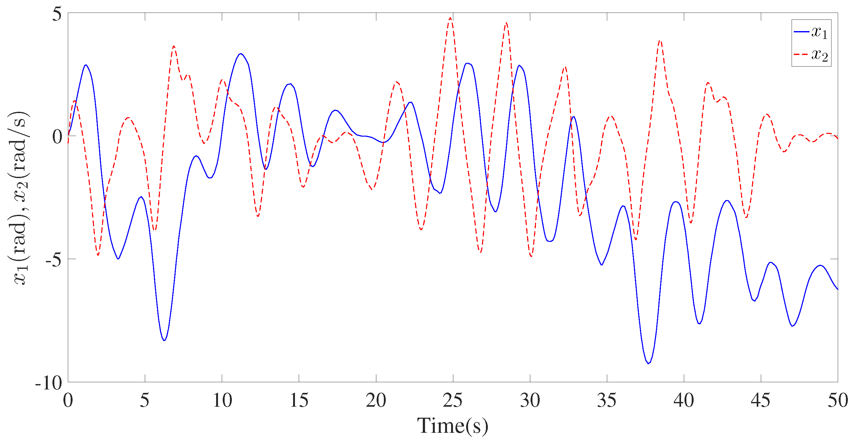
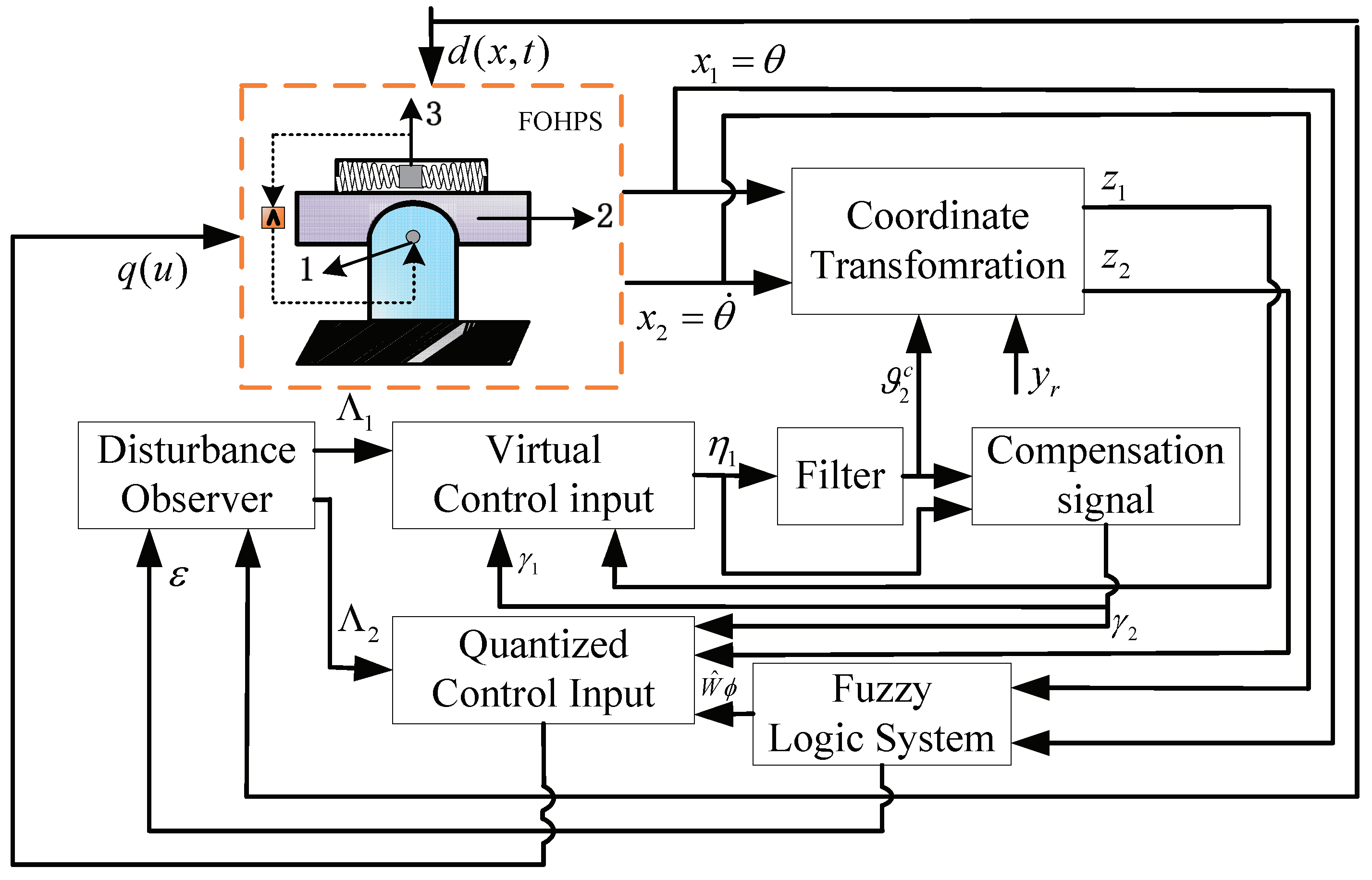
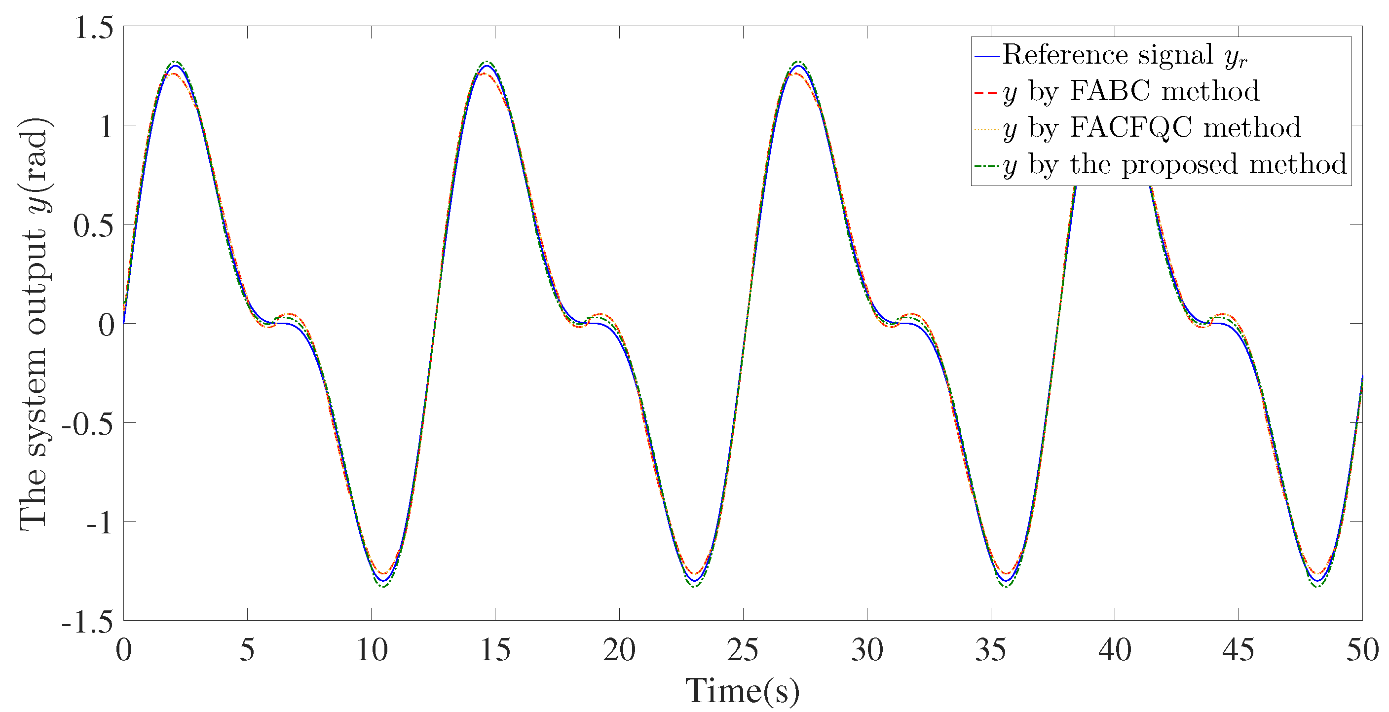
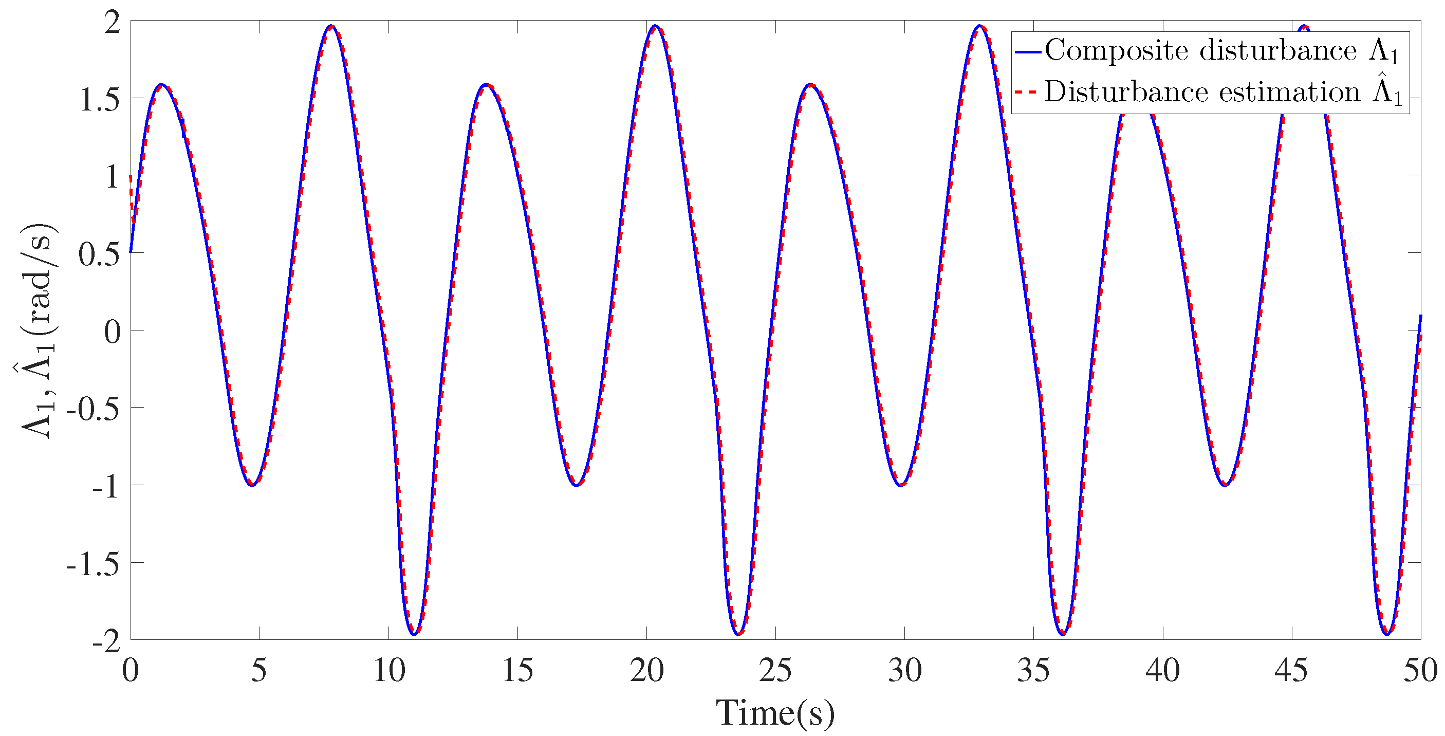
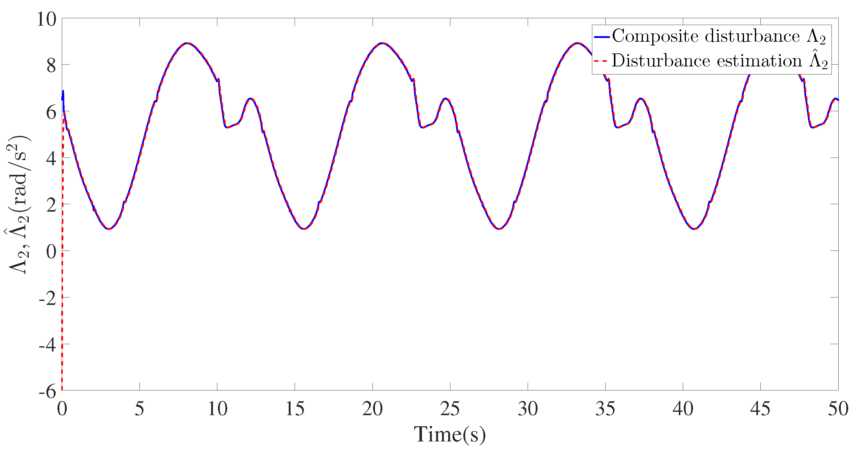
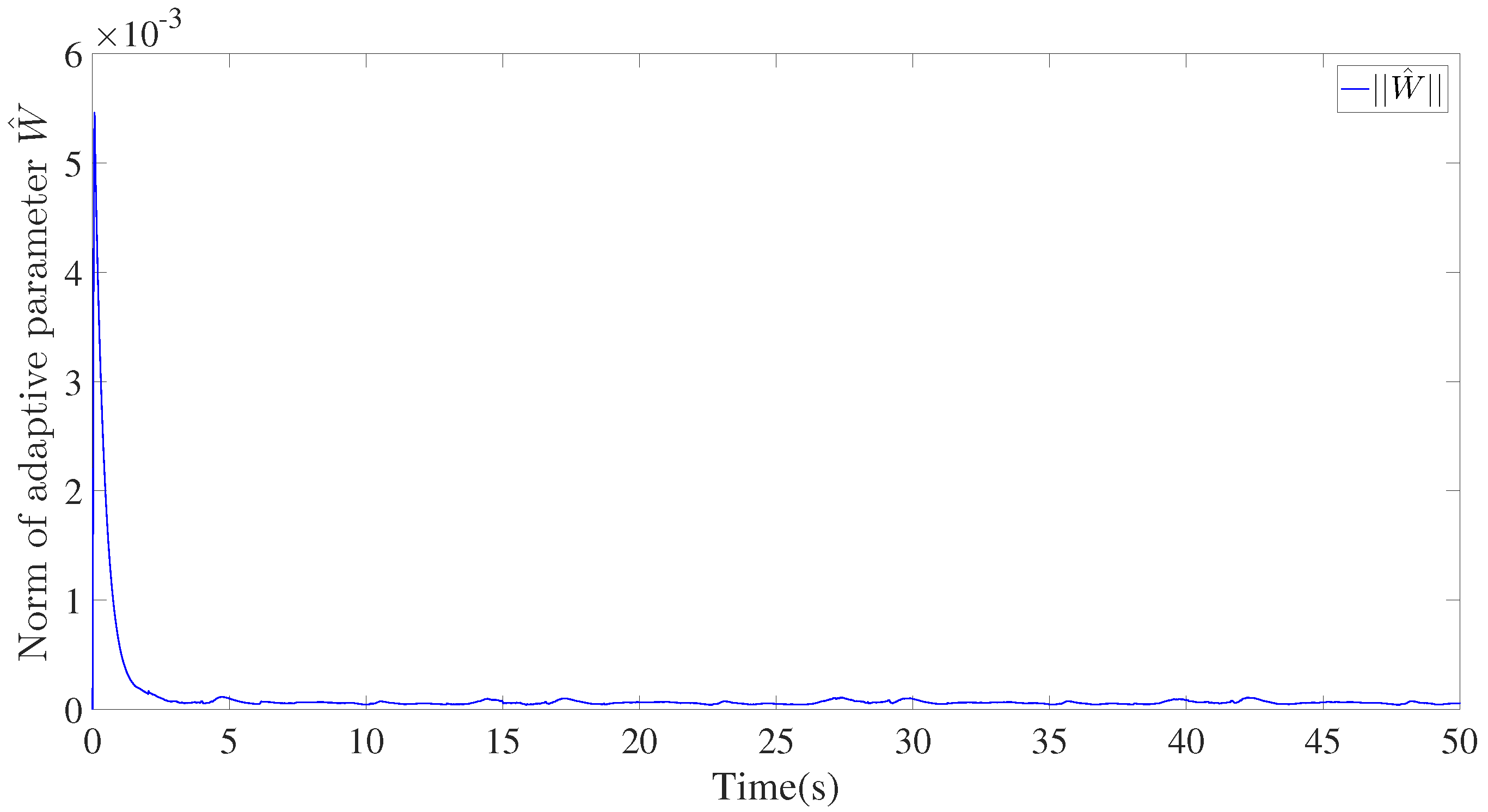
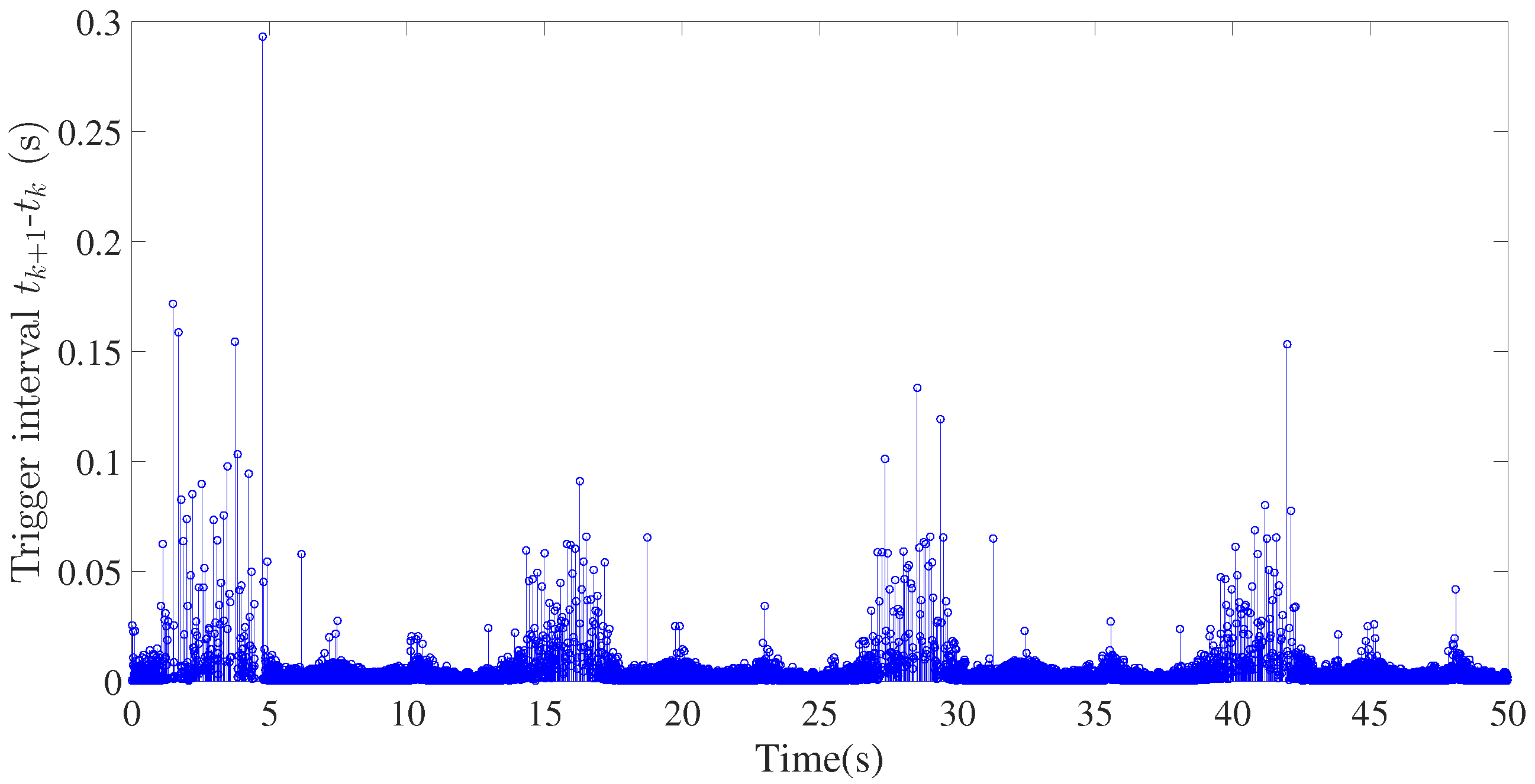
4. Simulation Verification

In this section, the effectiveness and the practical potential of the presented control approach will be verified through a horizontal platform system (HPS). According to [39], an HPS is mainly composed of two components, i.e., a platform and an accelerometer located on the platform, as shown in Figure 2. When the platform deviates from the horizon, the accelerometer will send an output signal to the torque generator, which generates a torque to invert the rotation of the platform about the rotational axis. The mathematical equation of the HPS is

$$A\ddot{\theta }+D\dot{\theta }+kgsin\theta -\frac{3g}{R}\left(B-C\right)cos\theta sin\theta =Fcos\omega t,$$

(85)

where $\theta$ is the rotation of the platform relative to the earth; $\dot{\theta }$ is the corresponding angular velocity; $Fcos\omega t$ is harmonic torque; $A,B$ and C are the inertia moment of the platform; D is the damping coefficient; k denotes the proportional constant of the accelerometer; and g is the acceleration constant of gravity. The descriptions of relevant parameters are presented in

Table 1. Parameter list of the HPS.

Parameters	Nomenclature	Value	Unit
A	Inertia moment of the platform around axis 1	0.3	$\mathrm{kg}·{\mathrm{m}}^2$
B	Inertia moment of the platform around axis 2	0.5	$\mathrm{kg}·{\mathrm{m}}^2$
C	Inertia moment of the platform around axis 3	0.2	$\mathrm{kg}·{\mathrm{m}}^2$
D	Damping coefficient	0.4	$\mathrm{kg}·{\mathrm{m}}^2·{\mathrm{s}}^{-1}$
F	Amplitude of the harmonic torque	3.4	$\mathrm{N}·\mathrm{m}$
g	Acceleration constant of gravity	9.8	$\mathrm{m}·{\mathrm{s}}^{-2}$
k	Proportional constant of the accelerometer	0.11559633	$\mathrm{kg}·\mathrm{m}·\mathrm{rad}$
R	Radius of the Earth	6,378,000	$\mathrm{m}$
$\omega$	Circular frequency of the harmonic torque	1.8	$\mathrm{rad}·{\mathrm{s}}^{-1}$

.

We define $x_1=\theta$ and $x_2=\dot{\theta }$; then, system (85) can be transformed into the following form:

$$\left\{\begin{array}{cc}\hfill {\dot{x}}_1=& x_2\hfill \\ \hfill {\dot{x}}_2=& -a{x}_2-bsin{x}_1+lcos{x}_{1}sin{x}_1+hcos\omega t\hfill \end{array}\right.$$

(86)

where $a=\frac{D}{A},b=\frac{kg}{A},l=\frac{3g}{RA}(B$-$C)$ and $h=\frac{F}{A}$.

Furthermore, considering that the fractional-order model may provide a more accurate description of physical behavior and the actual system is inevitably influenced by perturbations, the fractional-order model of HPS with input quantization and perturbations can be given by [40]

$$\left\{\begin{array}{cc}\hfill D^{\alpha }{x}_1=& x_2+d_1(x,t)\hfill \\ \hfill D^{\alpha }{x}_2=& -a{x}_2-bsin{x}_1+lcos{x}_{1}sin{x}_1+hcos\omega t+q\left(u\right)+d_2(x,t)\hfill \end{array}\right.$$

(87)

where $\alpha$ denotes fractional order satisfying $\alpha =0.95$, $d_i(x,t)$ denotes the unknown perturbation and $q\left(u\right)$ represents the quantized control signal to be designed. The state response of system (86) without control effort under initial condition $[x_1\left(0\right),x_2\left(0\right)]=[0.1,$−$0.1]$ is displayed in Figure 3.

The control parameters, initial conditions and disturbances are provided in

Table 2. Selection of simulation parameters.

Design Parameters	Disturbance Terms
$c_1=c_2=50,a_1=a_2={\rho }_2=2,\iota =0.01$, $\delta =0.2,\kappa =0.15,u_{min}=5,u_{Max}=8,l_1=10$, $l_2=20,b_1=b_2=1,\chi =0.5,\alpha =0.95$.	$d_1(x,t)=1.5sin\left(2t\right)+0.5cos\left(x_1{x}_2\right)$, $d_2(x,t)=1.5cos\left(2t\right)+0.5sin\left(x_1{x}_2\right).$
Initial Conditions
$x_1\left(0\right)=0.1$,$x_2\left(0\right)=$ −$0.1,{\gamma }_1\left(0\right)={\gamma }_2\left(0\right)=0,$ ${\widehat{\Lambda }}_1\left(0\right)={\widehat{\Lambda }}_2\left(0\right)=0,\widehat{W}\left(0\right)={\underset{9}{\underbrace{[0,0,\dots ,0]}}}^T.$
Reference Signal
$y_r=0.5sin\left(t\right)+sin\left(0.5t\right)$

. Obviously, the selection of parameters $\delta ,\kappa ,u_{min}$ and $u_{Max}$ can ensure the quantization condition (73) holds. To achieve an accurate approximation of nonlinear functions, the Gaussian membership functions of FLSs are selected as: ${\mu }_{F^i}\left(x\right)=exp[$ −$(x$ − ${i+5)}^2/4]$ with $i=1,\dots ,9$.

Based on the established control framework as shown in Figure 4, the comparative simulation results under different control schemes are demonstrated in Figure 5, Figure 6, Figure 7, Figure 8, Figure 9, Figure 10 and Figure 11. The tracking performances are shown in Figure 5 and Figure 6. Furthermore, three kinds of performance indexes, consisting of integral absolute error (IAE), integral time-weighted absolute error (ITAE) and integral square error (ISE), are introduced to quantify the tracking performance under different control methods. It can be concluded from Figure 4 and Figure 5 and

Table 3. Performance comparisons under different methods.

Performance Index	Items	FABC in [10]	FACFQC in [31]	Proposed
IAE	${\int }_0^T\left|z_1\left(t\right)\right|dt$	1.75	1.755	1.153
ITAE	${\int }_0^{T}t\left|z_1\left(t\right)\right|dt$	40.62	40.77	26.09
ISE	${\int }_0^T{z}_1^2\left(t\right)dt$	0.073	0.075	0.035

that better tracking performance can be achieved by using the proposed method in comparison to the FABC method proposed in [10] and the FACFQC method developed in [31]. The responses of composite disturbance ${\Lambda }_i$ and its estimation ${\widehat{\Lambda }}_i$ are plotted in Figure 7 and Figure 8. Figure 9 and Figure 10 depict the trajectories of the norm of adaptive parameter $\left|\right|\widehat{W}\left|\right|$ and the quantized control signal $q\left(u\right)$. The time interval of each event is demonstrated in Figure 11.

5. Conclusions

In this article, a nonlinear disturbance observer-based event-triggered adaptive command-filtered quantized control approach is developed for fractional-order nonlinear systems with unknown disturbances. By introducing the command-filtered backstepping technique into the recursive design procedure, the potential issue of computational complexity existing in [10] and the negative effect caused by filter error in [17] are successfully avoided. Furthermore, a fractional-order disturbance observer is designed to achieve disturbance estimation, which can improve system robustness against composite disturbances consisting of unknown disturbances and approximation in comparison to the existing recursive control schemes proposed in [10,17,31]. Moreover, differently from the common time-triggered control methods in [10,17,31], the event-triggered control mechanism and input quantization are considered simultaneously, which can save a large amount of communication bandwidth and provide a possible way to make a trade-off between tracking performance and control costs. Finally, the validity and superiority of the proposed method are verified by a fractional-order HPS. However, it should be pointed out that a preassigned transient and steady-state performance cannot be ensured although the design controller can guarantee a relatively satisfactory tracking performance. Therefore, one of our future research works is to propose an adaptive control scheme with assured transient and steady-state performance for fractional-order nonlinear systems.

References

1. Tejado, I.; Pérez, E.; Valério, D. Fractional calculus in economic growth modeling of the group of seven. Fract. Calc. Appl. Anal. 2019, 22, 139–157. [Google Scholar] [CrossRef]
2. Zhang, X.; Huang, W. Adaptive Neural Network Sliding Mode Control for Nonlinear Singular Fractional Order Systems with Mismatched Uncertainties. Fractal Fract. 2020, 4, 50. [Google Scholar] [CrossRef]
3. Zouari, F.; Ibeas, A.; Boulkroune, A.; Cao, J.; Arefi, M.M. Adaptive neural output-feedback control for nonstrict-feedback time-delay fractional-order systems with output constraints and actuator nonlinearities. Neural Netw. 2018, 105, 256–276. [Google Scholar] [CrossRef] [PubMed]
4. Bao, H.; Park, J.H.; Cao, J. Adaptive synchronization of fractional-order memristor-based neural networks with time delay. Nonlinear Dyn. 2015, 82, 1343–1354. [Google Scholar] [CrossRef]
5. Lin, C.; Chen, B.; Shi, P.; Yu, J. Necessary and sufficient conditions of observer-based stabilization for a class of fractional-order descriptor systems. Syst. Control. Lett. 2018, 112, 31–35. [Google Scholar] [CrossRef]
6. Coronel-Escamilla, A.; Gomez-Aguilar, J.F.; Stamova, I.; Santamaria, F. Fractional order controllers increase the robustness of closed-loop deep brain stimulation systems. Chaos Solut. Fractals 2020, 140, 110149. [Google Scholar] [CrossRef]
7. Luo, S.; Lewis, F.L.; Song, Y.; Ouakad, H.M.J. Accelerated adaptive fuzzy optimal control of three coupled fractional-order chaotic electromechanical transducers. IEEE Trans. Fuzzy Syst. 2021, 29, 1701–1714. [Google Scholar] [CrossRef]
8. Zouari, F.; Ibeas, A.; Boulkroune, A.; Cao, J.; Arefi, M.M. Neural network controller design for fractional-order systems with input nonlinearities and asymmetric time-varying Pseudo-state constraints. Chaos Solut. Fractals 2021, 144, 110742. [Google Scholar] [CrossRef]
9. Wei, Y.; Tse, P.W.; Yao, Z.; Wang, Y. Adaptive backstepping output feedback control for a class of nonlinear fractional order systems. Nonlinear Dyn. 2016, 86, 1047–1056. [Google Scholar] [CrossRef]
10. Liu, H.; Pan, Y.; Li, S.; Chen, Y. Adaptive fuzzy backstepping control of fractional-order nonlinear systems. IEEE Trans. Syst. Man Cybern. Syst. 2017, 47, 2209–2217. [Google Scholar] [CrossRef]
11. Li, Y.; Wang, Q.; Tong, S. Fuzzy adaptive fault-tolerant control of fractional-order nonlinear systems. IEEE Trans. Syst. Man Cybern. Syst. 2021, 51, 1372–1379. [Google Scholar] [CrossRef]
12. Yu, J.; Zhao, L.; Yu, H.; Lin, C.; Dong, W. Fuzzy finite-time command filtered control of nonlinear systems with input saturation. IEEE Trans. Cybern. 2018, 48, 2378–2387. [Google Scholar] [PubMed]
13. Li, Y.; Li, K.; Tong, S. Finite-time adaptive fuzzy output feedback dynamic surface control for MIMO nonstrict feedback systems. IEEE Trans. Fuzzy Syst. 2019, 27, 96–110. [Google Scholar] [CrossRef]
14. Qiu, J.; Sun, K.; Rudas, I.J.; Gao, H. Command filter-based adaptive NN control for MIMO nonlinear systems with full-state constraints and actuator hysteresis. IEEE Trans. Cybern. 2020, 50, 2905–2915. [Google Scholar] [CrossRef] [PubMed]
15. Niu, B.; Li, H.; Karimi, H.R. Adaptive NN dynamic surface controller design for nonlinear pure-feedback switched systems with time-delays and quantized input. IEEE Trans. Syst. Man Cybern. Syst. 2018, 48, 1676–1688. [Google Scholar] [CrossRef]
16. Liu, Y. Adaptive dynamic surface asymptotic tracking for a class of uncertain nonlinear systems. Int. J. Robust Nonlinear Control. 2018, 28, 1233–1245. [Google Scholar] [CrossRef]
17. Ma, Z.; Ma, H. Adaptive fuzzy backstepping dynamic surface control of strict-feedback fractional-order uncertain nonlinear systems. IEEE Trans. Fuzzy Syst. 2020, 28, 122–133. [Google Scholar] [CrossRef]
18. Song, S.; Zhang, B.; Song, X.; Zhang, Z. Neuro-fuzzy-based adaptive dynamic surface control for fractional-order nonlinear strict-feedback systems with input constraint. IEEE Trans. Syst. Man Cybern. Syst. 2021, 50, 3575–3586. [Google Scholar] [CrossRef]
19. Song, S.; Park, J.H.; Zhang, B.; Song, X. Observer-based adaptive hybrid fuzzy resilient control for fractional-order nonlinear systems with time-varying delays and actuator failures. IEEE Trans. Fuzzy Syst. 2021, 29, 471–485. [Google Scholar] [CrossRef]
20. Liu, H.; Pan, Y.; Cao, J. Composite learning adaptive dynamic surface control of fractional-order nonlinear systems. IEEE Trans. Cybern. 2020, 50, 2557–2567. [Google Scholar] [CrossRef]
21. Song, X.; Sun, P.; Song, S.; Stojanovic, V. Finite-time adaptive neural resilient DSC for fractional-order nonlinear large-scale systems against sensor-actuator faults. Nonlinear Dyn. 2023, 111, 12181–12196. [Google Scholar] [CrossRef]
22. Xu, B.; Sun, F.; Pan, Y.; Chen, B. Disturbance observer-based composite learning fuzzy control of nonlinear systems with unknown dead zones. IEEE Trans. Syst. Man Cybern. Syst. 2017, 47, 1854–1862. [Google Scholar] [CrossRef]
23. Chen, M.; Shao, S.; Shi, P. Disturbance-observer-based robust synchronization control for a class of fractional-order chaotic systems. IEEE Trans. Circuits Syst. II Express Briefs 2017, 64, 417–421. [Google Scholar] [CrossRef]
24. Min, H.; Xu, S.; Ma, Q.; Zhang, B.; Zhang, Z. Composite-observer-based output-feedback control for nonlinear time-delay systems with input saturation and its application. IEEE Trans. Ind. Electron. 2018, 65, 5856–5863. [Google Scholar] [CrossRef]
25. Hou, C.; Liu, X.; Wang, H. Adaptive fault tolerant control for a class of uncertain fractional-order systems based on disturbance observer. Int. J. Robust Nonlinear Control. 2020, 30, 3436–3450. [Google Scholar] [CrossRef]
26. Han, S.I. Fuzzy supertwisting dynamic surface control for MIMO strict-feedback nonlinear dynamic systems with supertwisting nonlinear disturbance observer and a new partial tracking error constraint. IEEE Trans. Fuzzy Syst. 2019, 27, 2101–2114. [Google Scholar] [CrossRef]
27. Wei, X.; Dong, L.; Zhang, H.; Hu, X.; Han, J. Adaptive disturbance observer-based control for stochastic systems with multiple heterogeneous disturbances. Int. J. Robust Nonlinear Control. 2019, 29, 5533–5549. [Google Scholar] [CrossRef]
28. Gao, Z.; Guo, G. Command-filtered fixed-time trajectory tracking control of surface vehicles based on a disturbance observer. Int. J. Robust Nonlinear Control. 2019, 29, 4348–4365. [Google Scholar] [CrossRef]
29. Liu, Z.; Wang, F.; Zhang, Y.; Chen, C.L.P. Fuzzy adaptive quantized control for a class of stochastic nonlinear uncertain systems. IEEE Trans. Cybern. 2016, 46, 524–534. [Google Scholar] [CrossRef]
30. Liu, W.; Lim, C.C.; Shi, P.; Xu, S. Backstepping fuzzy adaptive control for a class of quantized nonlinear systems. IEEE Trans. Fuzzy Syst. 2017, 25, 1090–1101. [Google Scholar] [CrossRef]
31. Song, S.; Park, J.H.; Zhang, B.; Song, X.; Zhang, Z. Adaptive command filtered neuro-fuzzy control design for fractional-order nonlinear systems with unknown control directions and input quantization. IEEE Trans. Syst. Man Cybern. Syst. 2021, 51, 7238–7249. [Google Scholar] [CrossRef]
32. Sui, S.; Chen, C.L.P.; Tong, S.; Feng, S. Finite-time adaptive quantized control of stochastic nonlinear systems with input quantization: A broad learning system based identification method. Int. J. Robust Nonlinear Control. 2020, 67, 8555–8565. [Google Scholar] [CrossRef]
33. Xing, L.; Wen, C.; Liu, Z.; Su, H.; Cai, J. Event-triggered adaptive control for a class of uncertain nonlinear system. IEEE Trans. Autom. Control. 2017, 62, 2071–2076. [Google Scholar] [CrossRef]
34. Song, X.; Wu, C.; Stojanovic, V.; Song, S. 1 bit encoding–decoding-based event-triggered fixed-time adaptive control for unmanned surface vehicle with guaranteed tracking performance. Control. Eng. Pract. 2023, 135, 105513. [Google Scholar] [CrossRef]
35. Hayakawaa, T.; Ishii, H.; Tsumurac, K. Adaptive quantized control for nonlinear uncertain systems. Syst. Control. Lett. 2009, 58, 625–632. [Google Scholar] [CrossRef]
36. Song, X.; Wang, M.; Ahn, C.K.; Song, S. Finite-time fuzzy bounded control for semilinear PDE systems with quantized measurements and Markov jump actuator failures. IEEE Trans. Cybern. 2009, 52, 5732–5743. [Google Scholar] [CrossRef] [PubMed]
37. Li, Y.; Chen, Y.; Podlubny, I. Mittag-Leffler stability of fractional order nonlinear dynamic systems. Automatica 2009, 45, 1965–1969. [Google Scholar] [CrossRef]
38. Li, Y.; Yang, G. Adaptive asymptotic tracking control of uncertain nonlinear systems with input quantization and actuator faults. Automatica 2016, 96, 23–29. [Google Scholar] [CrossRef]
39. Ge, Z.M.; Yu, T.C.; Chen, Y.S. Chaos synchronization of a horizontal platform system. J. Sound Vib. 2003, 268, 731–749. [Google Scholar] [CrossRef]
40. Aghababa, M.P. Chaotic behavior in fractional-order horizontal platform systems and its suppression using a fractional finite-time control strategy. J. Mech. Sci. Technol. 2014, 28, 1875–1880. [Google Scholar] [CrossRef]
Figure 1. Block diagram of the proposed control scheme.
Fractalfract 07 00810 g001
Figure 2. Model of the platform circles along the Earth.
Fractalfract 07 00810 g002
Figure 3. The state response of system (87) without control effort.
Fractalfract 07 00810 g003
Figure 4. Control framework of the FOHPS.
Fractalfract 07 00810 g004
Figure 5. The reference signal y r and the system output y under different control methods.
Fractalfract 07 00810 g005
Figure 6. The tracking error y- y r under different control methods.
Fractalfract 07 00810 g006
Figure 7. The composite disturbance Λ 1 and its estimation Λ ^ 1 .
Fractalfract 07 00810 g007
Figure 8. The composite disturbance Λ 2 and its estimation Λ ^ 2 .
Fractalfract 07 00810 g008
Figure 9. The norm of adaptive parameter | | W ^ | | .
Fractalfract 07 00810 g009
Figure 10. Quantized control signal q ( u ) .
Fractalfract 07 00810 g010
Figure 11. Trigger interval t k + 1 t k .
Fractalfract 07 00810 g011