Local Fuzzy Fractional Partial Differential Equations in the Realm of Fractal Calculus with Local Fractional Derivatives

Abstract

In this study, local fuzzy fractional partial differential equations (LFFPDEs) are considered using a hybrid local fuzzy fractional approach. Fractal model behavior can be represented using fuzzy partial differential equations (PDEs) with local fractional derivatives. The current methods are hybrids of the local fuzzy fractional integral transform and the local fuzzy fractional homotopy perturbation method (LFFHPM), the local fuzzy fractional Sumudu decomposition method (LFFSDM) in the sense of local fuzzy fractional derivatives, and the local fuzzy fractional Sumudu variational iteration method (LFFSVIM); these are applied when solving LFFPDEs. The working procedure shows how effective solutions for specific LFFPDEs can be obtained using the applied approaches. Moreover, we present a comparison of the local fuzzy fractional Laplace variational iteration method (LFFLIM), the local fuzzy fractional series expansion method (LFFSEM), the local fuzzy fractional variation iteration method (LFFVIM), and the local fuzzy fractional Adomian decomposition method (LFFADM), which are applied to obtain fuzzy fractional diffusion and wave equations on Cantor sets. To demonstrate the effectiveness of the used techniques, some examples are given. The results demonstrate the major advantages of the approaches, which are equally efficient and simple to use in order to solve fuzzy differential equations with local fractional derivatives.

1. Introduction

The concept of fuzzy theory [1] was originally introduced by Zadeh in 1965; it has been considered extensively from several different aspects of the theory and its applications, such as linguistic information systems and approximate reasoning in [2,3,4], fuzzy decision making and fuzzy logic in [5,6], fuzzy analysis in [7], and fuzzy topology in [8,9].

Many mathematicians are interested in fuzzy fractional differential equations (FFDEs) and fuzzy fractional calculus since these theories are helpful in determining uncertainty influenced by ambiguity and inaccuracy. The concepts of Riemann–Liouville, Caputo–Hadamard, Caputo–Katugampola, Caputo–Atangana–Baleanu, Caputo–Fabrizio derivatives, and Caputo fuzzy fractional integrals and/or derivative operators have been applied in the majority of articles presented to date on this topic (see [10,11,12,13,14,15,16,17,18,19,20,21,22]).

Local fractional calculus has garnered the interest of many scientists due to its efficient treatment of non-differentiable functions. Local fractional calculus (LFC) represents differential and integral functions on fractal sets in their generalized form. Recently, physicists and engineers have appreciated LFC in addition to mathematicians. Fractional calculus is a generalized version of traditional calculus that examines real-order integrals and derivatives. Particularly when inherent constraints on a system influence its dynamics, these types of fractional derivative operators model a wide range of real-world phenomena more accurately. The literature contains a multitude of formulations pertaining to fractional integrals and derivatives. Due to the nonlocal nature of these formulations, they cannot be used to investigate the characteristics of local scaling phenomena or local fractional differentiability. Kolwankar and Gangal [23] introduced the notion of local fractional derivatives a decade ago; these derivatives show several features of integer-order derivatives. However, they lose the memory properties implicit to the fractional-order derivatives. The local differential operators with fractal order have been applied as effective and powerful mathematical tools to simulate complex real-world problems, communicating physical observations and geometrical clarifications. The purpose of LFC is to investigate the differential properties of fractal objects and nowhere differentiable functions. The fractal properties are typically observed in aquifers, porous media, turbulence, and other phenomena.

The local fractional derivative and calculus theory have recently been introduced by Yang et al. [24]. This is based on fractal geometry and is the best method for the characterization of the non-differentiable function defined on Cantor sets by Yang and Hua [25]. Golmankhaneh et al. [26] used fractional calculus in generalized Newtonian mechanics, Maxwell’s equations, and Hamiltonian mechanics. This then led to the emergence of ordinary differential equations and PDEs relating to this new concept, which became known as local fractional differential equations (LFDEs) and local fractional PDEs. This prompted some researchers to use the aforementioned methods to solve this new type of equation, including the local fractional ADM (LFADM) by Yang et al. [27], the local fractional homotopy perturbation method (LFHPM) [28], the local fractional variational iteration method [25], the local fractional variational iteration transform method [29], the local fractional Laplace decomposition method [30], the Yang–Machado–Baleanu–Cattain wave method, the fractional sech function method [31], and the fractional sech function method [32].

In 1993, Watugala [33] introduced the Sumudu transformation, which was thought to be the first of its kind in this field. This transformation was used to solve problems in control engineering. For this transformation, we devised a difficult inverse formula [34]. Asiru employed the Sumudu transformation to solve integral equations and systems of discrete dynamic equations in his studies [35,36]. Belgacem and Karaballi [37] presented a comprehensive list of functions and properties of the Sumudu transformation.

Recently, scientists and engineers have applied the ADM in order to solve linear, nonlinear differential, and integral problems ([38,39,40,41,42]). Moreover, some researchers have considered the ADM with the Sumudu transform. Trushit and Ramakanta [43] used the Adomian decomposition Sumudu transform method (ADSTM). We investigated the fluctuations in the temperature distribution, efficiency, and efficacy of porous fins for different fractional orders, porous parameters, and convection parameters. Saadeh et al. [44] presented the modified double ARA–Sumudu decomposition method for the obtained PDEs.

J.H. He invented the VIM, which was successfully used to solve autonomous ODEs [45,46]. It has been proven that this methodology works well when dealing with a variety of issues. Similar to the way in which the Shehu transform method is used to modify this method, the updated methodology is known as the variational iteration transform method (VITM). This technique has been used to solve many problems; see [40,47,48]. Recently, many authors have presented the VIM with the Sumudu transform. Prakash et al. [49] proposed a new computational method that was used to solve the numerically nonlinear time-fractional Zakharov–Kuznetsov (FZK) equation in two dimensions. Anac et al. [50] presented approximations of solutions to random component time-fractional PDEs with Caputo derivatives using the new Sumudu transform iterative method (SUTIM).

The Laplace variational iteration method (LVIM) is a combination of the Laplace transform and VIM. Many scientific projects have considered this technique. Bhargava et al. [51] used the LVIM to obtain series solutions to fractional-order heat equations that appear in many engineering applications. Nadeem et al. [52] presented a new amendment to the LVIM for the solution of fourth-order parabolic PDEs with variable coefficients.

In 2015, Yang et al. [28] and Zhang et al. [53] proposed the LFHPM. To further obtain the solution for the local fractional Tricomi equation (LFTE), Singh et al. [54] proposed the local fractional homotopy perturbation Sumudu transform method (LFHPSTM). Furthermore, Zhao et al. [55] used LFHPSTM to look into the local fractional heat conduction equations in fractal media. Others [56,57,58] have conducted work based on the application of LFHPSTM. The present work focuses on using the local fuzzy fractional homotopy perturbation Sumudu transform method (LFFHPSTM) to solve a few LFFPDEs in the fractal domain. Numerical simulations based on computers have been carried out in order to clarify the basic structure of the physical models expressed by LFFPDEs. The local fractional Sumudu transform (LFST) and the LFHPM as discussed in [59] are combined to generate the LFHPSTM.

The contributions and novelty of this work can be summarized as follows:

• The LFFHPSTM is clearly advantageous in comparison to the local fuzzy fractional homotopy perturbation method and LFADM as it combines two powerful mathematical tools to solve nonlinear LFFDEs. The combination of LFFHPM with the local fuzzy fractional Sumudu transform (LFFST) produces faster computations than LFFHPM; hence, this combination saves time. Furthermore, without requiring linearization, perturbation, or discretization, this method provides a convergent series solution. The LFHPSTM does not involve rounding errors and so consumes less time. Further, by using He’s polynomials to solve nonlinear terms, this approach can handle nonlinear LFDEs. The novelty and uniqueness of this work arise from the fact that the hybrid method used has never been applied to the studied LFFPDEs in the recent past. The technique has two features: the first is that it decomposes nonlinear terms using He’s polynomials, and the second is that it produces closed-form series solutions with fast convergence. Furthermore, the LFFHPSTM does not require the solution of complex Adomian polynomials. These attributes are decisive in the selection of this method to solve LFFPDEs.
• For the purpose of solving linear LFFPDEs, the combination of the ADM and the Sumudu transform method in the context of the local fractional derivative proves to be rather successful. Utilizing the series form of the solution proposed by the algorithm, rapid convergence will occur towards the exact solution. It is evident from the findings that the LFFSDM produces very accurate solutions with a minimal number of iterations. Therefore, given the effectiveness and flexibility of the application, as demonstrated by the provided examples, the work concludes that the LFFSDM can be used for additional linear LFFPDEs of higher order.
• The coupling of the VIM and the Sumudu transform method in the sense of local fractional derivatives has been shown to be highly effective in solving linear and nonlinear LFFPDEs. The local fuzzy fractional Sumudu variational iteration method (LFFSVIM) is a user-friendly solution for such problems. This method combines two potent techniques to obtain exact or approximate solutions to linear–nonlinear LFFPDEs. The modified LFFSVIM is an alternative algorithm to solve linear–nonlinear LFFPDEs.
• The fuzzy diffusion and wave equations defined on Cantor sets under fractal conditions are solved using the LFFLVIM. The method is found to be both useful and efficient in analytical applications. The LFFSEM, LFFVIM, and LFFADM all provide solutions to the same set of problems. All four approaches yield similar results; hence, the LFFLVIM is used as a viable alternative to the more standard technique of obtaining approximate solutions to linear–nonlinear fuzzy fractional differential equations.

This work is structured as follows. Section 2 is dedicated to providing the necessary notations and fundamental definitions. In Section 3, we present some LFFPDEs that are treated using a hybrid local fuzzy fractional approach. In Section 4, we propose the comparison of some analytical techniques applied to obtain fuzzy fractional diffusion and wave equations on the Cantor set. Finally, the conclusions end the work.

2. Preliminaries

The set of fuzzy numbers can be denoted by ${\mathbb{E}}^1$, whereas normal, fuzzy convex, upper semi-continuous and compactly supported fuzzy sets can be defined on the real line. For $0<\lambda \le 1,$ set ${\left[\psi \right]}_{\lambda }=\{\vartheta \in R|\psi \left(\vartheta \right)\ge \lambda \},$ and ${\left[\psi \right]}_0=cl\{\vartheta \in R|\psi \left(\vartheta \right)>0\}.$ We explain ${\left[\psi \right]}_{\varrho }=[{\underline{\psi }}_{\varrho },{\overline{\psi }}_{\varrho }]$; consequently, if $\psi \in {\mathbb{E}}^1,$ the $\varrho$-level set ${\left[\psi \right]}_{\varrho }$ is a closed interval for all $\varrho \in [0,1],$ refs. [7]. Suppose that $\psi ,\hslash \in {\mathbb{E}}^1$ and $k\in R,$ and the addition and scalar multiplication are defined by

• ${[\psi +\hslash ]}_{\varrho }={\left[\psi \right]}_{\varrho }+{[\hslash ]}_{\varrho },$
• ${\left[k\psi \right]}_{\varrho }=k{\left[\psi \right]}_{\varrho }.$

The triangular fuzzy number defined as a fuzzy set in ${\mathbb{E}}^1,$ is determined by $\psi =(a,b,c)\in R$ and $a\le b\le c$ such that ${\underline{\psi }}_{\varrho }=a+(b-a)\varrho$ and ${\overline{\psi }}_{\varrho }=c-(c-b)\varrho$ are the endpoints of $\varrho$-level sets for all $\varrho \in [0,1].$ The support of fuzzy number $\psi$ is given as

$$\sup p\left(\psi \right)=cl\{\vartheta \in R|\psi \left(\vartheta \right)>0\},$$

where $cl$ is the closure of set $\{\vartheta \in R|\psi \left(\vartheta \right)>0\}.$

Definition 1

([60]). Let us consider $\psi ,\hslash \in {\mathbb{E}}^1$. If there exists a $w\in {\mathbb{E}}^1$ such that $\psi =\hslash +w$, then w is called the Hukuhara difference of $\psi ,\hslash$, and it is denoted using $\psi \ominus \hslash$. Note that

$$\psi \ominus \hslash \ne \psi +(-1)\hslash .$$

The Hausdorff distance between two fuzzy numbers is defined as $\mathcal{D}:{\mathbb{E}}^1\times {\mathbb{E}}^1\to {\mathbb{R}}^{+}\cup \left\{0\right\}$

$$\mathcal{D}(\psi ,\hslash )=\underset{\varrho \in [0,1]}{\sup }\max \{|{\underline{\psi }}_{\varrho }-{\underline{\hslash }}_{\varrho }|,|{\overline{\psi }}_{\varrho }-{\overline{\hslash }}_{\varrho }|\},$$

where the $\varrho$-level sets of $\psi$ and ℏ are ${\left[\psi \right]}_{\varrho }=({\underline{\psi }}_{\varrho },{\overline{\psi }}_{\varrho })$ and ${[\hslash ]}_{\varrho }=({\underline{\hslash }}_{\varrho },{\overline{\hslash }}_{\varrho })$, respectively. It is easy to note that $\mathcal{D}$ is a metric in ${\mathbb{E}}^1$ and $(\mathcal{D},{\mathbb{E}}^1)$ is a complete metric space [61]. The $\varrho$-level set of fuzzy functions $\psi :A\subseteq R\to {\mathbb{E}}^1$ can be represented by ${\left[\psi \left(\mu \right)\right]}_{\varrho }=[\underline{\psi }(\mu ,\varrho ),\overline{\psi }(\mu ,\varrho )],\mu \in A\subseteq R$ and $0\le \varrho \le 1.$

Definition 2

([62,63]). For arbitrary fuzzy numbers $\psi ,\hslash \in {\mathbb{E}}^1,\psi =[{\underline{\psi }}_{\varrho },{\overline{\psi }}_{\varrho }],\hslash =[{\underline{\hslash }}_{\varrho },{\overline{\hslash }}_{\varrho }]$, the quantity $D(\psi ,\hslash )={\sup }_{\varrho \in [0,1]}\max \{|{\underline{\psi }}_{\varrho }-{\underline{\hslash }}_{\varrho }|,|{\overline{\psi }}_{\varrho }-{\overline{\hslash }}_{\varrho }|\}$ is the distance between ψ and $\tilde{\hslash }$

• $({\mathbb{E}}^1,\mathcal{D})$ denote a complete metric space,
• $\mathcal{D}(\psi \oplus w,\hslash \oplus w)=\mathcal{D}(\psi ,\hslash ),\forall \psi ,\hslash ,w\in {\mathbb{E}}^1,$
• $\mathcal{D}(\psi \oplus \hslash ,w\oplus e)\le \mathcal{D}(\psi ,w)+\mathcal{D}(\hslash ,e),\forall \psi ,\hslash ,w,e\in {\mathbb{E}}^1$,
• $\mathcal{D}(\psi \oplus \hslash ,\tilde{0})\le \mathcal{D}(\psi ,\tilde{0})+\mathcal{D}(\hslash ,\tilde{0}),\forall \psi ,\hslash \in {\mathbb{E}}^1,$
• $\mathcal{D}(\rho \odot \psi ,\rho \odot \hslash )=|\rho |\mathcal{D}(\psi ,\hslash ),\forall \psi ,\hslash \in {\mathbb{E}}^1,\rho \in \mathbb{R},$
• $\mathcal{D}({\rho }_1\odot \psi ,{\rho }_2\odot \psi )=|{\rho }_1-{\rho }_2|\mathcal{D}(\psi ,\tilde{0}),\forall \psi \in {\mathbb{E}}^1,{\rho }_1,{\rho }_2\in \mathbb{R},$ with ${\rho }_1·{\rho }_2\ge 0$.

Let us consider the definition of the Hukuhara difference (H-difference) in [64]. The Hukuhara H-difference is proposed as a set w for which $\psi {\ominus }_{gH}\tilde{\hslash }=w\iff \psi =\hslash \oplus w$. The H-difference is unique; however, it does not always exist (a necessary condition for $\psi {\ominus }_{gH}\hslash$ to exist is that $\psi$ contains a translation $\left\{c\right\}\oplus \hslash of\hslash$).

Definition 3

([63,64]). The generalized Hukuhara difference between two fuzzy numbers $\psi ,\hslash \in {\mathbb{E}}^1$ is given as

$$\psi {\ominus }_{gH}\hslash =w\iff \left\{\begin{array}{ll}\hfill & \left(i\right)\psi =\hslash \oplus w,\hfill \\ \hfill & or\left(ii\right)\hslash =\psi \oplus (-w).\hfill \end{array}\right.$$

(1)

In terms of the ϱ-level, we obtain $[\psi {\ominus }_{gH}\hslash ]=[\min \{{\psi }_{\varrho }-{\underline{\hslash }}_{\varrho },{\overline{\psi }}_{\varrho }-{\overline{\hslash }}_{\varrho }\},\max \{{\underline{\psi }}_{\varrho }-{\underline{\hslash }}_{\varrho },{\overline{\psi }}_{\varrho }-{\overline{\hslash }}_{\varrho }\}]$, and if the H-difference exists, then $\psi \ominus \hslash =\psi {\ominus }_{gH}\hslash$; the conditions for the existence of $w=\psi {\ominus }_{gH}\hslash \in {\mathbb{E}}^1$ are

$$\begin{array}{cc}\hfill Case\left(i\right)& \left\{\begin{array}{cc}\hfill & {\underline{w}}_{\varrho }={\underline{\psi }}_{\varrho }-{\underline{\hslash }}_{\varrho }and{\overline{w}}_{\varrho }={\overline{\psi }}_{\varrho }-{\overline{\hslash }}_{\varrho },\forall \varrho \in [0,1],\hfill \\ \hfill & with{\underline{w}}_{\varrho }increasing,{\overline{w}}_{\varrho }decreasing,{\underline{w}}_{\varrho }\le {\overline{w}}_{\varrho }.\hfill \end{array}\right.\hfill \end{array}$$

(2)

$$\begin{array}{cc}\hfill Case\left(ii\right)& \left\{\begin{array}{cc}\hfill & {\underline{w}}_{\varrho }={\overline{\psi }}_{\varrho }-{\overline{\hslash }}_{\varrho }and{\overline{w}}_{\varrho }={\underline{\psi }}_{\varrho }-{\underline{\hslash }}_{\varrho },\forall \varrho \in [0,1],\hfill \\ \hfill & with{\underline{w}}_{\varrho }increasing,{\overline{w}}_{\varrho }decreasing,{\underline{w}}_{\varrho }\le {\overline{w}}_{\varrho }.\hfill \end{array}\right.\hfill \end{array}$$

(3)

It is simple to demonstrate that (i) and (ii) are both true provided that w is a crisp number.

Definition 4

([65]). Assume that $\psi (\vartheta ,\theta ):\mathcal{D}\to {\mathbb{E}}^1$ and $({\vartheta }_0,\theta )\in \mathcal{D}$. We say that ψ is strongly generalized Hukuhara differentiable on $({\vartheta }_0,\theta )$ (GH-differentiable for short) if there exists an element $\frac{\partial \psi }{\partial \vartheta }{|}_{({\vartheta }_0,\theta )}\in {\mathbb{E}}^1$ such that

(i) 

for all $\aleph >0$ sufficiently small, $\exists \psi ({\vartheta }_0+\aleph ,\theta ){\ominus }_H\psi ({\vartheta }_0,\theta ),\psi ({\vartheta }_0,t){\ominus }_H\psi ({\vartheta }_0-\aleph ,\theta )$ and the limits (in the metric D)

$$\underset{\aleph \to 0+}{\lim }\frac{\psi ({\vartheta }_0+\aleph ,\theta ){\ominus }_H\psi ({\vartheta }_0,\theta )}{\aleph }=\underset{\aleph \to 0+}{\lim }\frac{\psi ({\vartheta }_0,\theta ){\ominus }_H\psi ({\vartheta }_0-\aleph ,\theta )}{\aleph }=\frac{\partial \psi }{\partial \vartheta }{|}_{({\vartheta }_0,\theta )},$$

or

(ii) 

for all $\aleph >0$ sufficiently small, $\exists \psi ({\vartheta }_0,\theta ){\ominus }_H\psi ({\vartheta }_0+\aleph ,\theta ),\psi ({\vartheta }_0-\aleph ,\theta ){\ominus }_H\psi ({\vartheta }_0,\theta )$ and the limits

$$\underset{\aleph \to 0+}{\lim }\frac{\psi ({\vartheta }_0,\theta ){\ominus }_H\psi ({\vartheta }_0+\aleph ,\theta )}{-\aleph }=\underset{\aleph \to 0+}{\lim }\frac{\psi ({\vartheta }_0-\aleph ,\theta ){\ominus }_H\psi ({\vartheta }_0,\theta )}{-\aleph }=\frac{\partial \psi }{\partial \vartheta }{|}_{({\vartheta }_0,\theta )},$$

or

(iii) 

for all $\aleph >0$ sufficiently small, $\exists \psi ({\vartheta }_0+\aleph ,\theta ){\ominus }_H\psi ({\vartheta }_0,\theta ),\psi ({\vartheta }_0-\aleph ,\theta ){\ominus }_H\psi ({\vartheta }_0,\theta )$ and the limits

$$\underset{\aleph \to 0+}{\lim }\frac{\psi ({\vartheta }_0+\aleph ,\theta ){\ominus }_H\psi ({\vartheta }_0,\theta )}{\aleph }=\underset{\aleph \to 0+}{\lim }\frac{\psi ({\vartheta }_0-\aleph ,\theta ){\ominus }_H\psi ({\vartheta }_0,\theta )}{-\aleph }=\frac{\partial \psi }{\partial x}{|}_{({\vartheta }_0,\theta )},$$

or

(iv) 

for all $\aleph >0$ sufficiently small, $\exists \psi ({\vartheta }_0,\theta ){\ominus }_H\psi ({\vartheta }_0+\aleph ,\theta ),\psi ({\vartheta }_0,\theta ){\ominus }_H\psi ({\vartheta }_0-\aleph ,\theta )$ and the limits

$$\underset{\aleph \to 0+}{\lim }\frac{\psi ({\vartheta }_0,\theta ){\ominus }_H\psi ({\vartheta }_0+\aleph ,\theta )}{-\aleph }=\underset{h\to 0+}{\lim }\frac{\psi ({\vartheta }_0,\theta ){\ominus }_H\psi ({\vartheta }_0-\aleph ,\theta )}{\aleph }=\frac{\partial \psi }{\partial \vartheta }{|}_{({\vartheta }_0,\theta )}.$$

Definition 5

([64]). Assume that $\psi (\vartheta ,\theta ):\mathcal{D}\to {\mathbb{E}}^1$ is a function and set $\psi (\vartheta ,\theta )=\left[\right(\underline{\psi }(\vartheta ,\theta ;\varrho )$, $\overline{\psi }(\vartheta ,\theta ;\varrho )]$ for each $\varrho \in [0,1]$. Then,

(1) If ψ is gH-differentiable in the first form (i), then $\underline{\psi }(\vartheta ,\theta ;\varrho )$ and $\overline{\psi }(\vartheta ,\theta ;\varrho )$ are differentiable functions and

$${\left[\frac{\partial \psi }{\partial \vartheta }\right]}_{\varrho }=\left[\frac{\partial \underline{\psi }(\vartheta ,\theta ;\varrho )}{\partial \vartheta },\frac{\partial \overline{\psi }(\vartheta ,\theta ;\varrho )}{\partial \mu }\right],$$

(4)

(2) If ψ is gH-differentiable in the second form (ii), then $\overline{\psi }(\vartheta ,\theta ;\varrho )$ and $\underline{\psi }(\vartheta ,\theta ;\varrho )$ are differentiable functions and

$${\left[\frac{\partial \psi }{\partial \vartheta }\right]}_{\varrho }=\left[\frac{\partial \overline{\psi }(\vartheta ,\theta ;\varrho )}{\partial \vartheta },\frac{\partial \underline{\psi }(\vartheta ,\theta ;\varrho )}{\partial \vartheta }\right].$$

(5)

Definition 6

([66]). A fuzzy-valued function ψ of two variables is a rule that assigns to every ordered pair of real numbers, $(\vartheta ,\theta )$, in a set $\mathbb{D}$, a unique fuzzy number denoted by $\psi (\vartheta ,\theta )$. The set $\mathbb{D}$ is the domain of ψ and its range is the set of values that ψ takes on, which is $\left\{\psi \right(\vartheta ,\theta )|(\vartheta ,\theta )\in \mathbb{D}\}$. The parametric representation of the fuzzy-valued function $\psi :\mathbb{D}\to {\mathbb{E}}^1$ is expressed by $\psi (\vartheta ,\theta ;\sigma )=[\underline{\psi }(\vartheta ,\theta ;\varrho ),\overline{\psi }(\vartheta ,\theta ;\varrho )]$, for any $(\vartheta ,\theta )\in \mathbb{D}$ and $\varrho \in [0,1]$.

Definition 7

([66]). A fuzzy-valued function $\psi :[\varnothing ,\ell ]\to {\mathbb{E}}^1$ is said to be continuous at ${\theta }_0\in [\varnothing ,\ell ]$ if, for every positive ε, there is $\delta >0$ such that $\mathbb{D}\left(\psi \left(\theta \right),\psi \left({\theta }_0\right)\right)<\epsilon$ whenever $\left|\theta -{\theta }_0\right|<\delta .$ If ψ is continuous for each $\theta \in [\varnothing ,\ell ]$, then we say that ψ is fuzzy continuous on $[\varnothing ,\ell ].$

Next, we regard ${\mathcal{C}}^{\mathcal{F}}[\varnothing ,\ell ]$ as the space of all continuous fuzzy-valued functions on $[\varnothing ,\ell ]$, and we recall the space of all Lebesgue integrable fuzzy functions on the bounded interval $[\varnothing ,\ell ]\subset \mathbb{R}$ by ${\mathcal{L}}^{\mathcal{F}}[\varnothing ,\ell ]$, refs. [67].

Definition 8

([67]). Assume that $\psi \left(\mu \right)\in {\mathcal{C}}^{\mathcal{F}}[\varnothing ,\ell ]\cap {\mathcal{L}}^{\mathcal{F}}[\varnothing ,\ell ]$. The fuzzy Riemann–Liouville integral of fuzzy function ψ is given as

$$\left({\mathbb{I}}_{a+}^{\alpha }\psi \right)\left(\mu \right)=\frac{1}{\mathsf{\Gamma }\left(\alpha \right)}{\int }_{\varnothing }^{\mu }\frac{\psi \left(\iota \right)d\iota }{{(\mu -\iota )}^{1-\alpha }},\mu >\varnothing ,0<\alpha ⩽1.$$

Let the ϱ-level expression of a fuzzy function ψ as $f(\mu ;\varrho )=[\underline{\psi }(\mu ;\varrho ),\overline{\psi }(\mu ;\varrho )]$, for $0⩽\varrho ⩽1$.

Definition 9

([60,67]). Let $\psi \in {\mathcal{C}}^{\mathcal{F}}[\varnothing ,\ell ]\cap {\mathcal{L}}^{\mathcal{F}}[\varnothing ,\ell ]$ be fuzzy function and $0<\alpha \le 1$. Then, ψ is said to be Caputo gH-differentiable at μ when

$${}^{\mathcal{C}}{\mathcal{D}}_{\varnothing }^{\alpha }\psi (\mu ;\varrho )=\frac{1}{\mathsf{\Gamma }(1-\alpha )}{\int }_{{\mu }_0}^{\mu }{(\mu -\iota )}^{-\alpha }{\psi }^{\prime }(\iota ;\varrho )d\iota .$$

Note that, later, we indicate ${}^{\mathcal{C}}{\mathcal{D}}_0^{\alpha }\psi (\iota ;\varrho )$ using ${}^{\mathcal{C}}{\mathcal{D}}^{\alpha }\psi (\iota ;\varrho ).$

Theorem 1

([60]). Let $\psi \in C^{\mathcal{F}}[\varnothing ,\ell ]\cap L^{\mathcal{F}}[\varnothing ,\ell ],{\mu }_0\in (a,b)$ and $0<\alpha \le 1.$ Then,

(i) 

if ψ is an (i)-differentiable fuzzy function, then

$$\left({}_i^{\mathcal{C}}{\mathcal{D}}_{{\mu }_0}^{\alpha }\right)\psi (\mu ;\varrho )=\left[\left({}^{\mathcal{C}}{D}_{{\vartheta }_0}^{\alpha }\right)\underline{\psi }(\mu ;\varrho ),\left({}^{\mathcal{C}}{\mathcal{D}}_{{\mu }_0}^{\alpha }\right)\overline{\psi }(\mu ;\varrho )\right],0\le \varrho \le 1,$$

(ii) 

if ψ is an (ii)-differentiable fuzzy function, then

$$\left({}_{ii}^{\mathcal{C}}{\mathcal{D}}_{{\mu }_0}^{\alpha }\right)\psi (\mu ;\varrho )=\left[\left({}^{\mathcal{C}}{\mathcal{D}}_{{\mu }_0}^{\alpha }\right)\overline{\psi }(\mu ;\varrho ),\left({}^{\mathcal{C}}{\mathcal{D}}_{{\mu }_0}^{\alpha }\right)\underline{\psi }(\mu ;\varrho )\right],0\le \varrho \le 1.$$

Local Fractional Calculus

We present the local fractional calculus, refs. [24,27,68], as follows.

Definition 10.

The real-valued function $\mathbb{W}\left(\vartheta \right)$ is known local fractional continuous at $\vartheta ={\vartheta }_0$ and is displayed by ${\lim }_{\vartheta ={\vartheta }_0}\mathbb{W}\left(\vartheta \right)=\mathbb{W}\left({\vartheta }_0\right)$ if there exists a relation.

At $\vartheta ={\vartheta }_0$, the real-valued function $\mathbb{W}\left(\vartheta \right)$ is known as local fractional continuous and is shown by ${\lim }_{\vartheta ={\vartheta }_0}\mathbb{W}\left(\vartheta \right)=\mathbb{W}\left({\vartheta }_0\right)$ if ∃, if there is a relation.

$|\mathbb{W}\left(\vartheta \right)-\mathbb{W}\left({\vartheta }_0\right)|<{\delta }^{\beta },0<\beta \le 1$ with $|\vartheta -{\vartheta }_0|<\epsilon ,$ for $\epsilon ,\delta \in R.$ In the same way, $\mathbb{W}\left(\vartheta \right)$ is referred to as local fractional continuous on $({\gamma }_1,{\gamma }_2)$ and is symbolized as $\mathbb{W}\left(\vartheta \right)\in C_{\beta }({\gamma }_1,{\gamma }_2),$ provided that $|\mathbb{W}\left(\vartheta \right)-\mathbb{W}\left({\vartheta }_0\right)|<{\delta }^{\beta }$ holds for $\mathbb{W}\in ({\gamma }_1,{\gamma }_2).$

Definition 11.

Assume that $({\gamma }_1,{\gamma }_2),$ is the interval and $\mathsf{\Delta }\theta =\max \{\mathsf{\Delta }{\theta }_0,\mathsf{\Delta }{\theta }_1,\mathsf{\Delta }{\theta }_2,\cdots \}$ is a partition of $({\gamma }_1,{\gamma }_2),$ with $({\theta }_{\epsilon },{\theta }_{\epsilon +1})$, $\epsilon =0,1,2,\dots ,N-1,{\theta }_0={\gamma }_1,{\theta }_N={\gamma }_2$ with $\mathsf{\Delta }{\theta }_{\epsilon }={\theta }_{\epsilon +1}-{\theta }_{\epsilon }.$ Then, the local fractional integral of $\mathbb{W}\left(\vartheta \right)\in C_{\beta }({\gamma }_1,{\gamma }_2)$ is defined as

$$\begin{array}{c}\hfill {}_{{\gamma }_1}{I}_{{\gamma }_2}^{\beta }\mathbb{W}\left(\vartheta \right)=\frac{1}{\mathsf{\Gamma }(1+\beta )}{\int }_{{\gamma }_1}^{{\gamma }_2}\mathbb{W}\left(\theta \right){\left(d\theta \right)}^{\beta }=\frac{1}{\mathsf{\Gamma }(1+\beta )}\underset{\mathsf{\Delta }\theta \to 0}{\lim }\sum _{\epsilon =0}^{\mathbb{N}-1}\mathbb{W}\left({\theta }_{\epsilon }\right){\left(\mathsf{\Delta }{\theta }_{\epsilon }\right)}^{\beta }.\end{array}$$

(6)

Definition 12.

The Mittage–Leffler function in fractal media is represented as

$$\begin{array}{c}\hfill E_{\beta }\left({\vartheta }^{\beta }\right)=\sum _{m=0}^{\infty }\frac{{\vartheta }^{m\beta }}{\mathsf{\Gamma }(1+m\beta )},0<\beta \le 1.\end{array}$$

(7)

Definition 13.

In fractal media, the trigonometric function is stated as

$$\begin{array}{cc}\hfill {\sin }_{\beta }\left({\vartheta }^{\beta }\right)& =\sum _{m=0}^{\infty }{(-1)}^m\frac{{\vartheta }^{(2m+1)\beta }}{\mathsf{\Gamma }(1+(2m+1\left)\beta \right)}\hfill \\ \hfill {\cos }_{\beta }\left({\vartheta }^{\beta }\right)& =\sum _{m=0}^{\infty }{(-1)}^m\frac{{\vartheta }^{2m\beta }}{\mathsf{\Gamma }(1+2m\beta )},\vartheta \in R,0<\beta \le 1.\hfill \end{array}$$

Definition 14.

Assume that $W\left(\vartheta \right)$ satisfies the condition of local fractional continuity according to Definition 10. Hence, we have the inverse formula of the local fractional integral described in Definition 11 as

$$\begin{array}{c}\hfill {\mathbb{D}}_{\vartheta }^{\beta }\mathbb{W}\left({\vartheta }_0\right)=\frac{d^{\beta }\mathbb{W}\left({\vartheta }_0\right)}{d{\vartheta }^{\beta }}={\mathbb{W}}^{\beta }\left({\vartheta }_0\right)=\underset{\vartheta -{\vartheta }_0}{\lim }\frac{{\mathsf{\Delta }}^{\beta }(\mathbb{W}\left(\vartheta \right)-\mathbb{W}\left({\vartheta }_0\right))}{{(\vartheta -{\vartheta }_0)}^{\beta }},\vartheta \in ({\gamma }_1,{\gamma }_2),\end{array}$$

(8)

where ${\mathsf{\Delta }}^{\beta }(\mathbb{W}\left(\vartheta \right)-\mathbb{W}\left({\vartheta }_0\right))\cong \mathsf{\Gamma }(\beta +1)(\mathbb{W}\left(\vartheta \right)-\mathbb{W}\left({\vartheta }_0\right)),$ and ${\mathbb{D}}_{\vartheta }^{\beta }\mathbb{W}\left({\vartheta }_0\right)$ denote the local fractional derivative of $\mathbb{W}\left(\vartheta \right)\in C_{\beta }({\gamma }_1,{\gamma }_2)$ of order $\beta$ at $\vartheta ={\vartheta }_0.$

The local fractional partial derivative of $\mathbb{W}(\vartheta ,\xi )\in C_{\beta }({\gamma }_1,{\gamma }_2)$ of order $\beta$ was provided by Yang [24,68] as follows:

$$\begin{array}{c}\hfill \frac{{\partial }^{\beta }}{\partial {\xi }^{\beta }}\mathbb{W}(\vartheta ,\xi )=\frac{{\mathsf{\Delta }}^{\beta }(\mathbb{W}(\vartheta ,\xi )-\mathbb{W}(\vartheta ,{\xi }_0))}{{(\xi -{\xi }_0)}^{\beta }},\vartheta \in ({\gamma }_1,{\gamma }_2),\end{array}$$

(9)

where ${\mathsf{\Delta }}^{\beta }(\mathbb{W}(\vartheta ,\theta )-\mathbb{W}(\vartheta ,{\theta }_0)\cong \mathsf{\Gamma }(\beta +1)(\mathbb{W}(\vartheta ,\theta )-\mathbb{W}(\vartheta ,{\theta }_0))$.

This study makes use of the formulas for local fractional derivatives and local fractional integrals of a few spatial functionals that are listed in [24,68]: ${\mathbb{D}}_{\vartheta }^{\beta }a\mathbb{W}\left(\vartheta \right)=a{\mathbb{D}}_{\vartheta }^{\beta }\mathbb{W}\left(\vartheta \right)$, where a is constant

$$\begin{array}{cc}\hfill {\mathbb{D}}_{\vartheta }^{\beta }\left(\frac{{\vartheta }^{m\beta }}{\mathsf{\Gamma }(1+m\beta )}\right)& =\frac{{\vartheta }^{(m-1)\beta }}{\mathsf{\Gamma }(1+(m-1\left)\beta \right)},\hfill \\ \hfill {\mathbb{I}}_{\vartheta }^{\beta }\left(\frac{{\vartheta }^{m\beta }}{\mathsf{\Gamma }(1+m\beta )}\right)& =\frac{{\vartheta }^{(m+1)\beta }}{\mathsf{\Gamma }(1+(m+1\left)\beta \right)},m\in N,\hfill \end{array}$$

where ${\vartheta }^{\beta }$ specifies the Cantor function.

3. Local Fuzzy Fractional Partial Differential Equations

In this section, the hybrid fuzzy fractional approach is applied to some local fuzzy fractional partial differential equations.

3.1. Local Fractional Sumudu Transform

We introduce the following definitions of the local fractional Sumudu transform (LFST), refs. [59,69].

Definition 15.

The LFST of a function $\mathbb{W}\left(\theta \right)$ is given as

$$\begin{array}{c}\hfill LF{S}_{\beta }\left\{\mathbb{W}\left(\theta \right)\right\}={\overline{\mathbb{W}}}_{\beta }\left(z\right)=\frac{1}{\mathsf{\Gamma }(1+\beta )}{\int }_0^{\infty }{E}_{\beta }(-z^{-\beta }{\theta }^{\beta })\frac{\mathbb{W}\left(\theta \right)}{z^{\beta }}{\left(d\theta \right)}^{\beta },0<\beta \le 1.\end{array}$$

(10)

Applying the formula above, the inverse LFST is defined as

$$\begin{array}{c}\hfill LF{S}_{\beta }^{-1}\left\{{\overline{\mathbb{W}}}_{\beta }\left(z\right)\right\}=\mathbb{W}\left(\theta \right),0<\beta \le 1.\end{array}$$

(11)

Remark 1.

$LF{S}_{\beta }\left\{\frac{{\theta }^{\beta }}{\mathsf{\Gamma }(1+\beta )}\right\}=z^{\beta }.$

Theorem 2.

(Linearity). If $LF{S}_{\beta }\left\{\mathbb{W}\left(\theta \right)\right\}={\overline{\mathbb{W}}}_{\beta }\left(z\right)$ and $LF{S}_{\beta }\left\{V\left(\theta \right)\right\}={\overline{V}}_{\beta }\left(z\right),$ we get

$$\begin{array}{c}\hfill LF{S}_{\beta }\{\mathbb{W}\left(\theta \right)+V\left(\theta \right)\}={\overline{\mathbb{W}}}_{\beta }\left(z\right)+{\overline{\mathbb{V}}}_{\beta }\left(z\right),0<\beta \le 1.\end{array}$$

(12)

Theorem 3.

(Local fractional convolution). If $LF{S}_{\beta }\left\{\mathbb{W}\left(\theta \right)\right\}={\overline{\mathbb{W}}}_{\beta }\left(z\right)$ and $LF{S}_{\beta }\left\{\mathbb{V}\left(\theta \right)\right\}={\overline{V}}_{\beta }\left(z\right),$ we obtain

$LF{S}_{\beta }\{\mathbb{W}\left(\theta \right)\ast \mathbb{V}\left(\theta \right)\}=z^{\beta }{\overline{\mathbb{W}}}_{\beta }\left(z\right){\overline{\mathbb{V}}}_{\beta }\left(z\right)$ with $\mathbb{W}\left(\theta \right)\ast \mathbb{V}\left(\theta \right)=\frac{1}{\mathsf{\Gamma }(1+\beta )}{\int }_0^{\infty }\mathbb{W}\left(y\right)\mathbb{V}(\theta -y){\left(d\theta \right)}^{\beta }.$

Theorem 4.

If $LF{S}_{\beta }\left\{\mathbb{W}\left(\theta \right)\right\}={\overline{\mathbb{W}}}_{\beta }\left(z\right),$ then

$$\begin{array}{cc}\hfill LF{S}_{\beta }\left\{\frac{d^{\beta }\mathbb{W}\left(\theta \right)}{d{\theta }^{\beta }}\right\}& =\frac{{\overline{\mathbb{W}}}_{\beta }\left(z\right)-\mathbb{W}\left(0\right)}{z^{\beta }},\hfill \\ \hfill LF{S}_{\beta }\left\{\frac{d^{m\beta }\mathbb{W}\left(\theta \right)}{d{\theta }^{m\beta }}\right\}& =\frac{1}{z^{m\beta }}\left[{\overline{\mathbb{W}}}_{\beta }\left(z\right)-\sum _{k=0}^{m-1}{z}^{k\beta }{\mathbb{W}}^{k\beta }\left(0\right)\right].\hfill \end{array}$$

(13)

For $m=2,$ we obtain

$$\begin{array}{cc}\hfill LF{S}_{\beta }\left\{\frac{d^{2\beta }\mathbb{W}\left(\theta \right)}{d{\theta }^{2\beta }}\right\}& =\frac{1}{z^{2\beta }}\left[{\overline{\mathbb{W}}}_{\beta }\left(z\right)-\mathbb{W}\left(0\right)-z^{\beta }{\mathbb{W}}^{\beta }\left(0\right)\right],\hfill \end{array}$$

(14)

where ${\overline{\mathbb{W}}}_{\beta }\left(z\right)=LF{S}_{\beta }\left\{\mathbb{W}\left(\theta \right)\right\}.$

Theorem 5.

If $LF{S}_{\beta }\left\{\mathbb{W}\left(\theta \right)\right\}={\overline{\mathbb{W}}}_{\beta }\left(z\right),$ we obtain $LF{S}_{\beta }\left\{{}_0{I}_{\theta }^{\left(\beta \right)}\mathbb{W}\left(\theta \right)\right\}=z^{\beta }{\overline{\mathbb{W}}}_{\beta }\left(z\right).$

Theorem 6.

The LFST of some special functions

$$\begin{array}{c}\hfill LF{S}_{\beta }\left\{a\right\}=a,LF{S}_{\beta }\left\{E_{\beta }\left(a{\theta }^{\beta }\right)\right\}=\frac{1}{1-a{z}^{\beta }},\end{array}$$

(15)

where a is a constant.

$$\begin{array}{cc}\hfill LF{S}_{\beta }\left\{\frac{{\theta }^{\beta }}{\mathsf{\Gamma }(1+\beta )}\right\}& =z^{\beta },LF{S}_{\beta }\left\{\sum _{k=0}^{\infty }{a}_k{\theta }^{\beta k}\right\}=\sum _{k=0}^{\infty }\mathsf{\Gamma }(1+k\beta )a_k{z}^{\beta k},\hfill \\ \hfill LF{S}_{\beta }\left\{{\cos }_{\beta }\left(a{\theta }^{\beta }\right)\right\}& =\frac{1}{1+a^2{z}^{2\beta }},LF{S}_{\beta }\left\{{\sin }_{\beta }\left(a{\theta }^{\beta }\right)\right\}=\frac{a{z}^{\beta }}{1+a^2{z}^{2\beta }},\hfill \\ \hfill LF{S}_{\beta }\left\{{\sinh }_{\beta }\left(a{\theta }^{\beta }\right)\right\}& =\frac{a{z}^{\beta }}{1-a^2{z}^{2\beta }},LF{S}_{\beta }\left\{{\cosh }_{\beta }\left(a{\theta }^{\beta }\right)\right\}=\frac{a{z}^{\beta }}{1-a^2{z}^{2\beta }}.\hfill \end{array}$$

3.2. Local Fuzzy Fractional Homotopy Perturbation Sumudu Transform Method

We provide the fundamental plan for the LFFHPSTM. The following LFFPDEs are used to demonstrate the basic steps of the LFFHPSTM.

$$\begin{array}{c}\hfill {\mathbb{L}}_{\beta }\mathbb{W}(\vartheta ,\theta )\oplus {\mathbb{U}}_{\beta }\mathbb{W}(\vartheta ,\theta )\oplus {\mathbb{R}}_{\beta }\mathbb{W}(\vartheta ,\theta )=h(\vartheta ,\theta ),0<\vartheta <1,0<\theta <1,\end{array}$$

(16)

where ${\mathbb{L}}_{\beta }=\frac{{\partial }^{k\beta }}{\partial {\theta }^{k\beta }}$ is called the linear local fuzzy fractional differential operator (LFFDO) of order $k\beta ,{\mathbb{U}}_{\beta }$ is called the LFFDO of order less than ${\mathbb{L}}_{\beta },{\mathbb{R}}_{\beta }$ indicates the nonlinear local differential operator in $\vartheta$ and $\theta$ are variables, $\mathbb{W}(\vartheta ,\theta )$ specifies the unknown local fractional continuous function, and $h(\vartheta ,\theta )$ is called the nowhere differentiable source term.

Furthermore, the fundamental strategy of LFFHPSTM proposes the use of LFFST in Equation (16)

$$\begin{array}{c}\hfill LFF{S}_{\beta }\left[L_{\beta }\mathbb{W}(\vartheta ,\theta )\right]\oplus LFF{S}_{\beta }\left[U_{\beta }\mathbb{W}(\vartheta ,\theta )\right]\oplus LFF{S}_{\beta }\left[R_{\beta }\mathbb{W}(\vartheta ,\theta )\right]=LFF{S}_{\beta }\left[h(\vartheta ,\theta )\right].\end{array}$$

(17)

Using the property of LFFST, we have

$$\begin{array}{cc}\hfill {\mathbb{W}}_{\beta }(\vartheta ,z)& ={\mathbb{W}}_{\beta }(\vartheta ,0)\oplus z^{\beta }{\mathbb{W}}^{\beta }(\vartheta ,0)\oplus z^{2\beta }{\mathbb{W}}^{2\beta }(\vartheta ,0)\oplus \cdots \oplus z^{(k-1)\beta }{\mathbb{W}}^{(k-1)\beta }(\vartheta ,0)\hfill \\ \hfill & \ominus z^{k\beta }LFF{S}_{\beta }\left[U_{\beta }\mathbb{W}(\vartheta ,\theta )\right]\ominus z^{k\beta }LFF{S}_{\beta }\left[R_{\beta }\mathbb{W}(\vartheta ,\theta )\right]\oplus z^{k\beta }LFF{S}_{\beta }\left[R_{\beta }h(\vartheta ,\theta )\right],\hfill \end{array}$$

(18)

where ${\overline{W}}_{\beta }(\vartheta ,z)=LFF{S}_{\beta }\left[W(\vartheta ,\theta )\right],$ or

$$\begin{array}{cc}\hfill \mathbb{W}(\vartheta ,\theta )& =\sum _{m=0}^{k-1}{z}^{m\beta }\frac{{\partial }^{m\beta }\mathbb{W}(\vartheta ,0)}{\partial {\theta }^{m\beta }}\oplus z^{k\beta }LFF{S}_{\beta }\left[h(\vartheta ,\theta )\right]\ominus z^{k\beta }LFF{S}_{\beta }\left[{\mathbb{U}}_{\beta }(\vartheta ,\theta )\right]\ominus z^{k\beta }LFF{S}_{\beta }\left[R_{\beta }\mathbb{W}(\vartheta ,\theta )\right].\hfill \end{array}$$

(19)

Using Equation (19) and the reverse of LFFST, we obtain

$$\begin{array}{cc}\hfill \mathbb{W}(\vartheta ,\theta )& =\sum _{m=0}^{k-1}\frac{{\theta }^{m\beta }}{\mathsf{\Gamma }(1+m\beta )}\frac{{\partial }^{m\beta }\mathbb{W}(\vartheta ,0)}{\partial {\theta }^{m\beta }}\oplus LFF{S}_{\beta }^{-1}\left(z^{k\beta }LFF{S}_{\beta }\left[h(\vartheta ,\theta )\right]\right)\hfill \\ \hfill & \ominus LFF{S}_{\beta }^{-1}\left(z^{k\beta }LFF{S}_{\beta }\left[{\mathbb{U}}_{\beta }(\vartheta ,\theta )\right]\oplus z^{k\beta }LFF{S}_{\beta }\left[{\mathbb{R}}_{\beta }\mathbb{W}(\vartheta ,\theta )\right]\right).\hfill \end{array}$$

(20)

The basic steps include the following. The expansion of $\mathbb{W}(\vartheta ,\theta )$ takes the place of a power series of $\rho$ as

$$\begin{array}{cc}\hfill \mathbb{W}(\vartheta ,\theta )& =\sum _{n=0}^{\infty }{\rho }^{n\beta }{\mathbb{W}}_n(\vartheta ,\theta ),\hfill \end{array}$$

(21)

and the nonlinear component is presented as

$$\begin{array}{cc}\hfill {\mathbb{R}}_{\beta }\mathbb{W}(\vartheta ,\theta )& =\sum _{n=0}^{\infty }{\rho }^{n\beta }{\mathbb{H}}_n\left(\mathbb{W}\right),\hfill \end{array}$$

(22)

where $\rho (\vartheta ,\theta )$ is an embedding variable and ${\mathbb{H}}_n\left(\mathbb{W}\right)$ is a local fractional He’s polynomial represented as

$$\begin{array}{c}\hfill {\mathbb{H}}_n({\mathbb{W}}_0,{\mathbb{W}}_1,\dots ,{\mathbb{W}}_n)=\frac{1}{\mathsf{\Gamma }(n\beta +1)}\frac{{\partial }^{n\beta }}{\partial {\rho }^{n\beta }}{\left[{\mathbb{R}}_{\beta }\left(\sum _{i=0}^{\infty }{\rho }^{\beta i}{\mathbb{W}}_i\right)\right]}_{\rho =0},n=0,1,2,\dots \end{array}$$

(23)

Applying the values of $\mathbb{W}(\vartheta ,\theta )$ and ${\mathbb{R}}_{\beta }\mathbb{W}(\vartheta ,\theta )$ in Equation (20) yields the following homotopy equation:

$$\begin{array}{cc}\hfill \sum _{m=0}^{k-1}{\rho }^{n\beta }{\mathbb{W}}_n(\vartheta ,\theta )& =\sum _{m=0}^{k-1}\frac{{\theta }^{m\beta }}{\mathsf{\Gamma }(1+m\beta )}\frac{{\partial }^{m\beta }\mathbb{W}(\vartheta ,0)}{\partial {\theta }^{m\beta }}\oplus LFF{S}_{\beta }^{-1}\left(z^{k\beta }LFF{S}_{\beta }\left[h(\vartheta ,\theta )\right]\right)\hfill \\ \hfill & \ominus {\rho }^{\beta }LFF{S}_{\beta }^{-1}\left(z^{k\beta }LFF{S}_{\beta }\left({\mathbb{U}}_{\beta }\left[\sum _{n=0}^{\infty }{\rho }^{n\beta }{\mathbb{W}}_n(\vartheta ,\theta )\right]\right)\oplus z^{k\beta }LFF{S}_{\beta }\left[\sum _{n=0}^{\infty }{\rho }^{n\beta }{\mathbb{H}}_n\left(\mathbb{W}\right)\right]\right).\hfill \end{array}$$

(24)

Furthermore, comparing the coefficients of the same powers of $\rho$ yields

$$\begin{array}{c}\hfill \left\{\begin{array}{cc}\hfill & {\rho }^0:{\mathbb{W}}_0(\vartheta ,\theta )=\sum _{m=0}^{k-1}\frac{{\theta }^{m\beta }}{\mathsf{\Gamma }(1+m\beta )}\frac{{\partial }^{m\beta }\mathbb{W}(\vartheta ,0)}{\partial {\theta }^{m\beta }}\oplus LFF{S}_{\beta }^{-1}\left(z^{k\beta }LFF{S}_{\beta }\left[h(\vartheta ,\theta )\right]\right)\hfill \\ \hfill & {\rho }^{1\beta }:{\mathbb{W}}_1(\vartheta ,\theta )=-LFF{S}_{\beta }^{-1}\left(z^{k\beta }LFF{S}_{\beta }\left[{\mathbb{U}}_{\beta }\left({\mathbb{W}}_0(\vartheta ,\theta )\right)\oplus {\mathbb{H}}_0\left(\mathbb{W}\right)\right]\right)\hfill \\ \hfill & {\rho }^{2\beta }:{\mathbb{W}}_2(\vartheta ,\theta )=-LFF{S}_{\beta }^{-1}\left(z^{k\beta }LFF{S}_{\beta }\left[{\mathbb{U}}_{\beta }({\mathbb{W}}_1(\vartheta ,\theta )\oplus {\mathbb{H}}_1\left(\mathbb{W}\right)\right]\right)\hfill \\ \hfill & {\rho }^{3\beta }:{\mathbb{W}}_3(\vartheta ,\theta )=-LFF{S}_{\beta }^{-1}\left(z^{k\beta }LFF{S}_{\beta }\left[{\mathbb{U}}_{\beta }\left({\mathbb{W}}_2(\vartheta ,\theta )\right)\oplus {\mathbb{H}}_2\left(\mathbb{W}\right)\right]\right)\hfill \\ \hfill & ⋮.\hfill \end{array}\right.\end{array}$$

(25)

Finally, the local fractional series solution of Equation (16) can be written as

$$\begin{array}{cc}\hfill \mathbb{W}(\vartheta ,\theta )& =\underset{\mathbb{N}\to \infty }{\lim }\sum _{n=0}^{\mathbb{N}}{\mathbb{W}}_n(\vartheta ,\theta ).\hfill \end{array}$$

(26)

Convergence Analysis

We consider the Banach space $C[0,\mathcal{T}]$ of all continuous fuzzy functions on $[0,\mathcal{T}]$ with the supremum norm. Throughout this section, we consider $\mathbb{W}(\vartheta ,\theta ),{\mathbb{W}}_n(\vartheta ,\theta )\in C[0,\mathcal{T}].$

Theorem 7.

The solution obtained by the LFFHPSTM of fuzzy partial differential Equation (16) has a unique solution, whenever $0<\zeta <1.$

Proof. 

The solution of Equation (16) is of the form $\mathbb{W}(\vartheta ,\theta )={\sum }_{n=0}^{\infty }{\rho }^{n\beta }{\mathbb{W}}_n(\vartheta ,\theta ).$ Here,

$$\begin{array}{cc}\hfill \underline{\mathbb{W}}(\vartheta ,\theta ;\varrho )& =\sum _{k=0}^{n-1}\frac{{\theta }^k}{k!}{\underline{\mathbb{W}}}^{\left(k\right)}(\vartheta ,0)\left(\varrho \right)+LFF{S}_{\beta }^{-1}\left\{w^{n\beta }\left(LFF{S}_{\beta }\left\{\underline{h}(\vartheta ,\theta ;\varrho )-{\mathbb{U}}_{\beta }\underline{\mathbb{W}}(\vartheta ,\theta ;\varrho )-{\mathbb{R}}_{\beta }\underline{\mathbb{W}}(\vartheta ,\theta ;\varrho )\right\}\right)\right\},\hfill \\ \hfill \overline{\mathbb{W}}(\vartheta ,\theta ;\varrho )& =\sum _{k=0}^{n-1}\frac{{\theta }^k}{k!}{\overline{\mathbb{W}}}^{\left(k\right)}(\vartheta ,0)\left(\varrho \right)+LFF{S}_{\beta }^{-1}\left\{w^{n\beta }\left(LFF{S}_{\beta }\left\{\overline{h}(\vartheta ,\theta ;\varrho )-{\mathbb{U}}_{\beta }\overline{\mathbb{W}}(\vartheta ,\theta ;\varrho )-{\mathbb{R}}_{\beta }\overline{\mathbb{W}}(\vartheta ,\theta ;\varrho )\right\}\right)\right\},\hfill \end{array}$$

where $\varrho \in [0,1].$

Assume that $\mathbb{W}(\vartheta ,\theta )$ and $\mathbb{Y}(\vartheta ,\theta )$ are the distinct solutions of Equation (16); then,

$$\begin{array}{cc}\hfill |\underline{\mathbb{W}}(\vartheta ,\theta ;\varrho )-\underline{\mathbb{Y}}(\vartheta ,\theta ;\varrho )|& =|-LFF{S}_{\beta }^{-1}[w^{n\beta }\left(LFF{S}_{\beta }\left[U\right(\underline{\mathbb{W}}(\vartheta ,\theta ;\varrho )-\underline{\mathbb{Y}}(\vartheta ,\theta ;\varrho )\right)\hfill \\ \hfill & +R\left(\underline{\mathbb{W}}(\vartheta ,\theta ;\varrho )-\underline{\mathbb{Y}}(\vartheta ,\theta ;\varrho )\left)\right]\right)]|,\hfill \end{array}$$

(27)

$$\begin{array}{cc}\hfill |\overline{\mathbb{W}}(\vartheta ,\theta ;\varrho )-\overline{\mathbb{Y}}(\vartheta ,\theta ;\varrho )|& =|-LFF{S}_{\beta }^{-1}[w^{n\beta }\left(LFF{S}_{\beta }\left[U\right(\overline{\mathbb{W}}(\vartheta ,\theta ;\varrho )-\overline{\mathbb{Y}}(\vartheta ,\theta ;\varrho )\right)\hfill \\ \hfill & +R\left(\overline{\mathbb{W}}(\vartheta ,\theta ;\varrho )-\overline{\mathbb{Y}}(\vartheta ,\theta ;\varrho )\left)\right]\right)]|.\hfill \end{array}$$

(28)

Applying the convolution theorem,

$$\begin{array}{cc}\hfill |\underline{\mathbb{W}}(\vartheta ,\theta ;\varrho )-\underline{\mathbb{Y}}(\vartheta ,\theta ;\varrho )|& \le {\int }_0^{\theta }(|[U(\underline{\mathbb{W}}(\vartheta ,\theta ;\varrho )-\underline{\mathbb{Y}}(\vartheta ,\theta ;\varrho ))|\hfill \\ \hfill & +|R\left(\underline{\mathbb{W}}(\vartheta ,\theta ;\varrho )-\underline{\mathbb{Y}}(\vartheta ,\theta ;\varrho )\right)]|)\left|\frac{{(\theta -\eta )}^n}{n!}\right|d\eta \hfill \\ \hfill & \le {\int }_0^{\theta }(\mu |[(\underline{\mathbb{W}}(\vartheta ,\theta ;\varrho )-\underline{\mathbb{Y}}(\vartheta ,\theta ;\varrho ))|\hfill \\ \hfill & +\delta |\left(\underline{\mathbb{W}}(\vartheta ,\theta ;\varrho )-\underline{\mathbb{Y}}(\vartheta ,\theta ;\varrho )\right)]|)\left|\frac{{(\theta -\eta )}^n}{n!}\right|d\eta ,\hfill \end{array}$$

(29)

and

$$\begin{array}{cc}\hfill |\overline{\mathbb{W}}(\vartheta ,\theta ;\varrho )-\overline{\mathbb{Y}}(\vartheta ,\theta ;\varrho )|& \le {\int }_0^{\theta }(|[U(\overline{\mathbb{W}}(\vartheta ,\theta ;\varrho )-\overline{\mathbb{Y}}(\vartheta ,\theta ;\varrho ))|\hfill \\ \hfill & +|R\left(\overline{\mathbb{W}}(\vartheta ,\theta ;\varrho )-\overline{\mathbb{Y}}(\vartheta ,\theta ;\varrho )\right)]|)\left|\frac{{(\theta -\eta )}^n}{n!}\right|d\eta \hfill \\ \hfill & \le {\int }_0^{\theta }(\mu |[(\overline{\mathbb{W}}(\vartheta ,\theta ;\varrho )-\overline{\mathbb{Y}}(\vartheta ,\theta ;\varrho ))|\hfill \\ \hfill & +\delta |\left(\overline{\mathbb{W}}(\vartheta ,\theta ;\varrho )-\overline{\mathbb{Y}}(\vartheta ,\theta ;\varrho )\right)]|)\left|\frac{{(\theta -\eta )}^n}{n!}\right|d\eta .\hfill \end{array}$$

(30)

U is a bounded operator,

$$\begin{array}{cc}\hfill & |U\underline{\mathbb{W}}(\vartheta ,\theta ;\varrho )-\underline{\mathbb{Y}}(\vartheta ,\theta ;\varrho )|\le \mu |\underline{\mathbb{W}}(\vartheta ,\theta ;\varrho )-\underline{\mathbb{Y}}(\vartheta ,\theta ;\varrho )|\hfill \\ \hfill & |U\overline{\mathbb{W}}(\vartheta ,\theta ;\varrho )-\overline{\mathbb{Y}}(\vartheta ,\theta ;\varrho )|\le \mu |\overline{\mathbb{W}}(\vartheta ,\theta ;\varrho )-\overline{\mathbb{Y}}(\vartheta ,\theta ;\varrho )|\hfill \end{array}$$

and R satisfies the Lipschitz condition with $\delta >0$ such that

$$\begin{array}{cc}\hfill & |R\underline{\mathbb{W}}(\vartheta ,\theta ;\varrho )-\underline{\mathbb{Y}}(\vartheta ,\theta ;\varrho )|\le \delta |\underline{\mathbb{W}}(\vartheta ,\theta ;\varrho )-\underline{\mathbb{Y}}(\vartheta ,\theta ;\varrho )|\hfill \\ \hfill & |R\overline{\mathbb{W}}(\vartheta ,\theta ;\varrho )-\overline{\mathbb{Y}}(\vartheta ,\theta ;\varrho )|\le \delta |\overline{\mathbb{W}}(\vartheta ,\theta ;\varrho )-\overline{\mathbb{Y}}(\vartheta ,\theta ;\varrho )|\hfill \end{array}$$

$$\begin{array}{cc}\hfill |\underline{\mathbb{W}}(\vartheta ,\theta ;\varrho )-\underline{\mathbb{Y}}(\vartheta ,\theta ;\varrho )|& \le {\int }_0^{\theta }(\mu +\delta )|\underline{\mathbb{W}}(\vartheta ,\theta ;\varrho )-\underline{\mathbb{Y}}(\vartheta ,\theta ;\varrho )|\left|\frac{{(\theta -\eta )}^n}{n!}\right|d\eta \hfill \\ \hfill |\overline{\mathbb{W}}(\vartheta ,\theta ;\varrho )-\overline{\mathbb{Y}}(\vartheta ,\theta ;\varrho )|& \le {\int }_0^{\theta }(\mu +\delta )|\overline{\mathbb{W}}(\vartheta ,\theta ;\varrho )-\overline{\mathbb{Y}}(\vartheta ,\theta ;\varrho )|\left|\frac{{(\theta -\eta )}^n}{n!}\right|d\eta .\hfill \end{array}$$

Using the value theorem of integral calculus,

$$\begin{array}{cc}\hfill |\underline{\mathbb{W}}(\vartheta ,\theta ;\varrho )-\underline{\mathbb{Y}}(\vartheta ,\theta ;\varrho )|& \le (\mu +\delta )|\underline{\mathbb{W}}(\vartheta ,\theta ;\varrho )-\underline{\mathbb{Y}}(\vartheta ,\theta ;\varrho )|\mathcal{MT},\hfill \\ \hfill |\overline{\mathbb{W}}(\vartheta ,\theta ;\varrho )-\overline{\mathbb{Y}}(\vartheta ,\theta ;\varrho )|& \le (\mu +\delta )|\overline{\mathbb{W}}(\vartheta ,\theta ;\varrho )-\overline{\mathbb{Y}}(\vartheta ,\theta ;\varrho )|\mathcal{MT},\hfill \end{array}$$

where $\mathcal{M}=\max {(\theta -\eta )}^n$ and $\theta \in [0,\mathcal{T}].$

Hence,

$$\begin{array}{cc}\hfill |\underline{\mathbb{W}}(\vartheta ,\theta ;\varrho )-\underline{\mathbb{Y}}(\vartheta ,\theta ;\varrho )|& \le |\underline{\mathbb{W}}(\vartheta ,\theta ;\varrho )-\underline{\mathbb{Y}}(\vartheta ,\theta ;\varrho )|\zeta ,\hfill \\ \hfill |\overline{\mathbb{W}}(\vartheta ,\theta ;\varrho )-\overline{\mathbb{Y}}(\vartheta ,\theta ;\varrho )|& \le |\overline{\mathbb{W}}(\vartheta ,\theta ;\varrho )-\overline{\mathbb{Y}}(\vartheta ,\theta ;\varrho )|\zeta ,\hfill \end{array}$$

where $\zeta =(n+\delta )\mathcal{MT}$. Then,

$$\begin{array}{cc}\hfill (1-\zeta )|\underline{\mathbb{W}}(\vartheta ,\theta ;\varrho )-\underline{\mathbb{Y}}(\vartheta ,\theta ;\varrho )|& \le 0,\hfill \\ \hfill (1-\zeta )|\overline{\mathbb{W}}(\vartheta ,\theta ;\varrho )-\overline{\mathbb{Y}}(\vartheta ,\theta ;\varrho )|& \le 0,\hfill \end{array}$$

implies $\mathbb{W}(\vartheta ,\theta )=\mathbb{Y}(\vartheta ,\theta )$ whenever $0<\zeta <1.$ □

Theorem 8.

Assume ${\sum }_{n=0}^{\infty }{\mathbb{W}}_n\to \mathbb{W}$ if $\exists \zeta \in (0,1)$ such that $\parallel {\mathbb{W}}_n\parallel \le \zeta \parallel {\mathbb{W}}_{n-1}\parallel n\in \mathbb{N}$.

Proof. 

For the convergence of sequence $\left\{S_n(\vartheta ,\theta )\right\}$ of the partial sums of the series (26), we prove that $\left\{S_n(\vartheta ,\theta )\right\}$ is a Cauchy sequence in $\left(C\right[0,\mathcal{T}],\parallel ).$ As

$$\begin{array}{cc}\hfill \parallel {\underline{S}}_{n+1}(\vartheta ,\theta ;\varrho )-{\underline{S}}_n(\vartheta ,\theta ;\varrho )\parallel & =\parallel {\underline{\mathbb{W}}}_{n+1}(\vartheta ,\theta ;\varrho )\parallel \le \zeta \parallel {\underline{\mathbb{W}}}_n(\vartheta ,\theta ;\varrho )\parallel \hfill \\ \hfill & \le {\zeta }^2\parallel {\underline{\mathbb{W}}}_{n-1}(\vartheta ,\theta ;\varrho )\parallel \le \cdots \le {\zeta }^{n+1}\parallel {\underline{\mathbb{W}}}_0(\vartheta ,\theta ;\varrho )\parallel \hfill \end{array}$$

(31)

and

$$\begin{array}{cc}\hfill \parallel {\overline{S}}_{n+1}(\vartheta ,\theta ;\varrho )-{\overline{S}}_n(\vartheta ,\theta ;\varrho )\parallel & =\parallel {\overline{\mathbb{W}}}_{n+1}(\vartheta ,\theta ;\varrho )\parallel \le \zeta \parallel {\overline{\mathbb{W}}}_n(\vartheta ,\theta ;\varrho )\parallel \hfill \\ \hfill & \le {\zeta }^2\parallel {\overline{\mathbb{W}}}_{n-1}(\vartheta ,\theta ;\varrho )\parallel \le \cdots \le {\zeta }^{n+1}\parallel {\overline{\mathbb{W}}}_0(\vartheta ,\theta ;\varrho )\parallel \hfill \end{array}$$

(32)

Hence,

$$\begin{array}{cc}\hfill \parallel {\underline{S}}_n(\vartheta ,\theta ;\varrho )-{\underline{S}}_m(\vartheta ,\theta ;\varrho )\parallel & =\parallel \sum _{i=m+1}^n{\underline{\mathbb{W}}}_i(\vartheta ,\theta ;\varrho )\parallel \le \sum _{i=m+1}^n\parallel {\underline{\mathbb{W}}}_i(\vartheta ,\theta ;\varrho )\parallel \hfill \\ \hfill & \le {\zeta }^{m+1}\left(\sum _{i=0}^{n-m-1}{\zeta }^i\right)\parallel {\underline{\mathbb{W}}}_0(\vartheta ,\theta ;\varrho )\parallel \hfill \\ \hfill & ={\zeta }^{m+1}\frac{(1-{\zeta }^{n-m})}{1-\zeta }\parallel {\underline{\mathbb{W}}}_0(\vartheta ,\theta ;\varrho )\parallel ,n,m\in \mathbb{N},\hfill \end{array}$$

and

$$\begin{array}{cc}\hfill \parallel {\overline{S}}_n(\vartheta ,\theta ;\varrho )-{\overline{S}}_m(\vartheta ,\theta ;\varrho )\parallel & =\parallel \sum _{i=m+1}^n{\overline{\mathbb{W}}}_i(\vartheta ,\theta ;\varrho )\parallel \le \sum _{i=m+1}^n\parallel {\overline{\mathbb{W}}}_i(\vartheta ,\theta ;\varrho )\parallel \hfill \\ \hfill & \le {\zeta }^{m+1}\left(\sum _{i=0}^{n-m-1}{\zeta }^i\right)\parallel {\overline{\mathbb{W}}}_0(\vartheta ,\theta ;\varrho )\parallel \hfill \\ \hfill & ={\zeta }^{m+1}\frac{(1-{\zeta }^{n-m})}{1-\zeta }\parallel {\overline{\mathbb{W}}}_0(\vartheta ,\theta ;\varrho )\parallel ,n,m\in \mathbb{N}.\hfill \end{array}$$

since $0<\zeta <1$. Hence,

$$\begin{array}{c}\hfill \parallel {\underline{S}}_n(\vartheta ,\theta ;\varrho )-{\underline{S}}_m(\vartheta ,\theta ;\varrho )\parallel \le \frac{{\zeta }^{m+1}}{1-\zeta }\parallel {\underline{\mathbb{W}}}_0(\vartheta ,\theta ;\varrho )\parallel ,\\ \hfill \parallel {\overline{S}}_n(\vartheta ,\theta ;\varrho )-{\overline{S}}_m(\vartheta ,\theta ;\varrho )\parallel \le \frac{{\zeta }^{m+1}}{1-\zeta }\parallel {\overline{\mathbb{W}}}_0(\vartheta ,\theta ;\varrho )\parallel .\end{array}$$

Moreover, ${\mathbb{W}}_0(\vartheta ,\theta )$ is bounded; therefore, $\parallel S_{n+1}(\vartheta ,\theta )-S_n(\vartheta ,\theta )\parallel \to 0$ as $m,n\to \infty$. Thus, $\left\{S_n(\vartheta ,\theta )\right\}$ is a Cauchy sequence in $C[0,\mathcal{T}]$, and ${\sum }_{n=0}^{\infty }{\mathbb{W}}_n(\vartheta ,\theta )$ is convergent. □

3.3. Local Fuzzy Fractional Sumudu Decomposition Method

In this section, we present the fuzzy linear operator with a local fractional derivative as follows,

$$\begin{array}{c}\hfill {\mathbb{L}}_{\beta }\mathbb{U}(\vartheta ,\theta )\oplus {\mathbb{R}}_{\beta }\mathbb{U}(\vartheta ,\theta )=g(\vartheta ,\theta )\end{array}$$

(33)

where ${\mathbb{L}}_{\beta }=\frac{{\partial }^{m\beta }}{\partial t^{m\beta }}(m\in {\mathbb{N}}^{*})$ represents the linear local fuzzy fractional derivative operator of order $m\beta ,{\mathbb{R}}_{\beta }$ represents the linear local fuzzy fractional derivative operator of order less than $L_{\beta }$, and $g(\vartheta ,\theta )$ is a non-differentiable source term. Taking the local fractional Sumudu transform (denoted by $LFF{S}_{\beta }$) on both sides of Equation (33), we obtain

$$\begin{array}{c}\hfill LFF{S}_{\beta }\left[{\mathbb{L}}_{\beta }\mathbb{U}(\vartheta ,\theta )\right]\oplus LFF{S}_{\beta }\left[{\mathbb{R}}_{\beta }\mathbb{U}(\vartheta ,\theta )\right]=LFF{S}_{\beta }\left[g(\vartheta ,\theta )\right].\end{array}$$

(34)

Applying the prosperity of the local fractional Sumudu transform,

$$\begin{array}{c}\hfill \mathbb{U}(\vartheta ,\theta )=\sum _{k=0}^{m-1}{u}^{kv}\frac{{\partial }^{kv}\mathbb{U}(r,0)}{\partial {\theta }^{kv}}\frac{{\theta }^{kv}}{\mathsf{\Gamma }(1+kv)}+LFF{S}_{\beta }^{-1}\left(u^{mv}\left(LFFS\left[g(\vartheta ,\theta )\right]\right)\right)-LFF{S}_{\beta }^{-1}\left(u^{mv}\left(LFFS\left[{\mathbb{R}}_{\beta }\mathbb{U}(\vartheta ,\theta )\right]\right)\right).\end{array}$$

(35)

The unknown function U is then divided into infinite series by

$$\begin{array}{cc}\hfill \mathbb{W}(\vartheta ,\theta )& =\sum _{n=0}^{\infty }{\mathbb{W}}_n(\vartheta ,\theta ).\hfill \end{array}$$

(36)

Substituting (36) into (35), we obtain

$$\begin{array}{cc}\hfill \sum _{n=0}^{\infty }{\mathbb{W}}_n(\vartheta ,\theta )& =\sum _{m=0}^{k-1}\left[\frac{{\theta }^{m\beta }}{\mathsf{\Gamma }(1+m\beta )}\frac{{\partial }^{m\beta }\mathbb{W}(\vartheta ,0)}{\partial {\theta }^{m\beta }}\right]\oplus LFF{S}_{\beta }^{-1}\left(z^{k\beta }\left(LFF{S}_{\beta }\left[g(\vartheta ,\theta )\right]\right)\right)\hfill \\ \hfill & \ominus LFF{S}_{\beta }^{-1}\left(z^{k\beta }\left(LFF{S}_{\beta }\left[{\mathbb{R}}_{\beta }\sum _{n=0}^{\infty }{\mathbb{W}}_n(\vartheta ,\theta )\right]\right)\right).\hfill \end{array}$$

(37)

On comparing Equation (37), we obtain

$$\begin{array}{c}\hfill \left\{\begin{array}{cc}\hfill & {\mathbb{W}}_0(\vartheta ,\theta )=\sum _{m=0}^{k-1}\left[\frac{{\theta }^{m\beta }}{\mathsf{\Gamma }(1+m\beta )}\frac{{\partial }^{m\beta }\mathbb{W}(\vartheta ,0)}{\partial {\theta }^{m\beta }}\right]\oplus LFF{S}_{\beta }^{-1}\left(z^{k\beta }\left(LFF{S}_{\beta }\left[g(\vartheta ,\theta )\right]\right)\right),\hfill \\ \hfill & {\mathbb{W}}_1(\vartheta ,\theta )=-LFF{S}_{\beta }^{-1}\left(z^{k\beta }\left(LFF{S}_{\beta }\left[{\mathbb{U}}_{\beta }\left({\mathbb{W}}_0(\vartheta ,\theta )\right)\right]\right)\right),\hfill \\ \hfill & {\mathbb{W}}_2(\vartheta ,\theta )=-LFF{S}_{\beta }^{-1}\left(z^{k\beta }\left(LFF{S}_{\beta }\left[{\mathbb{U}}_{\beta }({\mathbb{W}}_1(\vartheta ,\theta )\right]\right)\right),\hfill \\ \hfill & {\mathbb{W}}_3(\vartheta ,\theta )=-LFF{S}_{\beta }^{-1}\left(z^{k\beta }\left(LFF{S}_{\beta }\left[{\mathbb{U}}_{\beta }\left({\mathbb{W}}_2(\vartheta ,\theta )\right)\right]\right)\right),\hfill \\ \hfill & ⋮.\hfill \end{array}\right.\end{array}$$

(38)

The general form of the local fractional recursive relation is

$$\begin{array}{cc}\hfill {\mathbb{W}}_0(\vartheta ,\theta )& =\sum _{m=0}^{k-1}\left[\frac{{\theta }^{m\beta }}{\mathsf{\Gamma }(1+m\beta )}\frac{{\partial }^{m\beta }\mathbb{W}(\vartheta ,0)}{\partial {\theta }^{m\beta }}\right]\oplus LFF{S}_{\beta }^{-1}\left(z^{k\beta }\left(LFF{S}_{\beta }\left[g(\vartheta ,\theta )\right]\right)\right),\hfill \\ \hfill {\mathbb{W}}_n(\vartheta ,\theta )& =-LFF{S}_{\beta }^{-1}\left(z^{k\beta }\left(LFF{S}_{\beta }\left[U_{\beta }\left({\mathbb{W}}_{n-1}(\vartheta ,\theta )\right)\right]\right)\right),\hfill \end{array}$$

(39)

where $0<v\le 1,n\in {\mathbb{N}}^{*}$ and $m=1,2,3,\dots$

3.4. Local Fuzzy Fractional Sumudu Variational Iteration Method

We consider the following nonlinear fuzzy operator with a local fractional derivative as

$$\begin{array}{c}\hfill {\mathbb{L}}_{\beta }\mathbb{W}(\vartheta ,\theta )\oplus {\mathbb{U}}_{\beta }\mathbb{W}(\vartheta ,\theta )\oplus {\mathbb{R}}_{\beta }\mathbb{W}(\vartheta ,\theta )=h(\vartheta ,\theta ),\end{array}$$

(40)

where ${\mathbb{L}}_{\beta }=\frac{{\partial }^{2\beta }}{\partial {\theta }^{2\beta }}$ specifies the linear local fuzzy fractional differential operator of order $2\beta$, ${\mathbb{U}}_{\beta }$ is called the linear local fuzzy fractional derivative operator of order less than in ${\mathbb{L}}_{\beta }$, ${\mathbb{N}}_{\beta }$ is represent the nonlinear local fractional operator, and $h(\vartheta ,\theta )$ is a non-differentiable source term. Using the LFFST of Equation (40), we obtain

$$\begin{array}{c}\hfill LFF{S}_{\beta }\left[L_{\beta }\mathbb{W}(\vartheta ,\theta )\right]\oplus LFF{S}_{\beta }\left[{\mathbb{U}}_{\beta }\mathbb{W}(\vartheta ,\theta )\right]\oplus LFF{S}_{\beta }\left[R_{\beta }\mathbb{W}(\vartheta ,\theta )\right]=LFF{S}_{\beta }\left[h(\vartheta ,\theta )\right].\end{array}$$

(41)

Applying the property of the LFFST, we obtain

$$\begin{array}{cc}\hfill LFF{S}_{\beta }\left[\mathbb{W}(\vartheta ,\theta )\right]& =\mathbb{W}(\vartheta ,0)\oplus {\mathbb{W}}_{\theta }^{\left(\beta \right)}(\vartheta ,0)u^{\beta }\oplus u^{2\beta }LFF{S}_{\beta }\left[h(\vartheta ,\theta )\right]\hfill \\ \hfill & \ominus u^{2\beta }LFF{S}_{\beta }\left[{\mathbb{N}}_{\beta }\mathbb{W}(\vartheta ,\theta )\oplus {\mathbb{R}}_{\beta }\mathbb{W}(\vartheta ,\theta )\right].\hfill \end{array}$$

(42)

Using the inverse LFFST of Equation (42) yields

$$\begin{array}{cc}\hfill \mathbb{W}(\vartheta ,\theta )& =\mathbb{W}(\vartheta ,0)\oplus {\mathbb{W}}_{\theta }^{\left(\beta \right)}(\vartheta ,0)\frac{{\theta }^{\beta }}{\mathsf{\Gamma }(1+\beta )}\hfill \\ \hfill & \oplus LFF{S}_{\beta }^{-1}\left(u^{2\beta }LFF{S}_{\beta }\left[\mathbb{W}(\vartheta ,\theta )\ominus {\mathbb{N}}_{\beta }\mathbb{W}(\vartheta ,\theta )\oplus {\mathbb{R}}_{\beta }\mathbb{W}(\vartheta ,\theta )\right]\right).\hfill \end{array}$$

(43)

Taking $\frac{{\partial }^{\beta }}{\partial {\theta }^{\beta }}$ of Equation (43), we obtain

$$\begin{array}{c}\hfill \frac{{\partial }^{\beta }\mathbb{W}(\vartheta ,\theta )}{\partial {\theta }^{\beta }}\ominus {\mathbb{W}}_{\theta }^{\left(\beta \right)}(\vartheta ,0)\oplus LFF{S}_{\beta }^{-1}\left(u^{2\beta }LFF{S}_{\beta }\left[{\mathbb{N}}_{\beta }{\mathbb{W}}_n(\vartheta ,\theta )\oplus {\mathbb{R}}_{\beta }{\mathbb{W}}_n(\vartheta ,\theta )\ominus h(\vartheta ,\theta )\right]\right)=0.\end{array}$$

(44)

The following limit is used to determine the solution

$$\begin{array}{c}\hfill \mathbb{W}(\vartheta ,\theta )=\underset{\vartheta \to \infty }{\lim }{\mathbb{W}}_n(\vartheta ,\theta ).\end{array}$$

(45)

3.5. Examples

In this part, we present the application of LFFHPSTM for local fuzzy fractional partial differential equations.

Example 1.

We consider the following local fuzzy fractional differential equation on Cantor:

$$\begin{array}{c}\hfill \frac{{\partial }^{\beta }\mathbb{W}(\vartheta ,\theta )}{\partial {\theta }^{\beta }}\oplus \frac{{\partial }^{2\beta }\mathbb{W}(\vartheta ,\theta )}{\partial {\vartheta }^{2\beta }}\ominus \mathbb{W}(\vartheta ,\theta )=0,\theta >0,\vartheta \in R,0<\beta \le 1,\end{array}$$

(46)

with the initial condition

$$\begin{array}{c}\hfill \mathbb{W}(\vartheta ,0)=\left[{(2.5+0.5\varrho )}^n,{(3.5-0.5\varrho )}^n\right]\odot {\sin }_{\beta }\left({\vartheta }^{\beta }\right),\end{array}$$

(47)

where $n=1,2,3,\dots$

1. Local fuzzy fractional homotopy perturbation Sumudu transform method

Using Equation (46) and the LFFST operator LFFS, we obtain

$$\begin{array}{c}\hfill LFF{S}_{\beta }\left[\frac{{\partial }^{\beta }\mathbb{W}(\vartheta ,\theta )}{\partial {\theta }^{\beta }}\right]\oplus LFF{S}_{\beta }\left[\frac{{\partial }^{2\beta }\mathbb{W}(\vartheta ,\theta )}{\partial {\vartheta }^{2\beta }}\right]=LFF{S}_{\beta }\left(W(\vartheta ,\theta )\right).\end{array}$$

(48)

Applying the LFFST for the LFFD formula to Equation (48) yields

$$\begin{array}{c}\hfill LFF{S}_{\beta }\left[\frac{{\partial }^{2\beta }\mathbb{W}(\vartheta ,\theta )}{\partial {\vartheta }^{2\beta }}\right]\oplus \frac{1}{z^{\beta }}\left[LFF{S}_{\beta }\left(\mathbb{W}(\vartheta ,\theta )\right)\ominus \mathbb{W}(\vartheta ,0)\right]=LFF{S}_{\beta }\left(\mathbb{W}(\vartheta ,\theta )\right).\end{array}$$

(49)

Rearranging the terms in Equation (48) yields

$$\begin{array}{c}\hfill LFF{S}_{\beta }\left(\mathbb{W}(\vartheta ,\theta )\right)=\mathbb{W}(\vartheta ,0)\oplus z^{\beta }LFF{S}_{\beta }\left(\mathbb{W}(\vartheta ,\theta )\right)\ominus z^{\beta }LFF{S}_{\beta }\left[\frac{{\partial }^{2\beta }\mathbb{W}(\vartheta ,\theta )}{\partial {\vartheta }^{2\beta }}\right].\end{array}$$

(50)

Further simplification on account of Equation (47) reduces Equation (50) to

$$\begin{array}{c}\hfill LFF{S}_{\beta }\left(\mathbb{W}(\vartheta ,\theta )\right)=\left[{(2.5+0.5\varrho )}^n,{(3.5-0.5\varrho )}^n\right]\odot {\sin }_{\beta }\left({\vartheta }^{\beta }\right)\oplus z^{\beta }LFF{S}_{\beta }\left(\mathbb{W}(\vartheta ,\theta )\right)\ominus z^{\beta }LFF{S}_{\beta }\left[\frac{{\partial }^{2\beta }\mathbb{W}(\vartheta ,\theta )}{\partial {\vartheta }^{2\beta }}\right].\end{array}$$

(51)

Using the inverse LFFST of Equation (51), we obtain

$$\begin{array}{cc}\hfill \mathbb{W}(\vartheta ,\theta )& =\left[{(2.5+0.5\varrho )}^n,{(3.5-0.5\varrho )}^n\right]\odot {\sin }_{\beta }\left({\vartheta }^{\beta }\right)\oplus LFF{S}_{\beta }^{-1}\left[z^{\beta }LFF{S}_{\beta }\left(\mathbb{W}(\vartheta ,\theta )\right)\right]\hfill \\ \hfill & \ominus LFF{S}_{\beta }^{-1}\left[z^{\beta }LFF{S}_{\beta }\left(\frac{{\partial }^{2\beta }\mathbb{W}(\vartheta ,\theta )}{\partial {\vartheta }^{2\beta }}\right)\right].\hfill \end{array}$$

(52)

The LFHPM suggests the following homotopy equation:

$$\begin{array}{cc}\hfill \sum _{n=0}^{\infty }{\rho }^{n\beta }{\mathbb{W}}_n(\vartheta ,\theta )& =\left[{(2.5+0.5\varrho )}^n,{(3.5-0.5\varrho )}^n\right]\odot {\sin }_{\beta }\left({\vartheta }^{\beta }\right)\oplus {\rho }^{\beta }LFF{S}_{\beta }^{-1}\left[z^{\beta }LFF{S}_{\beta }\left(\sum _{n=0}^{\infty }{\rho }^{n\beta }{\mathbb{W}}_n(\vartheta ,\theta )\right)\right]\hfill \\ \hfill & \ominus {\rho }^{\beta }LFF{S}_{\beta }^{-1}\left[z^{\beta }LFF{S}_{\beta }\left(\frac{{\partial }^{2\beta }\left\{{\sum }_{n=0}^{\infty }{\rho }^{n\beta }{\mathbb{W}}_n(\vartheta ,\theta )\right\}}{\partial {\vartheta }^{2\beta }}\right)\right].\hfill \end{array}$$

(53)

Comparing the like powers of $\rho$, we obtain

$$\begin{array}{c}\hfill \left\{\begin{array}{cc}\hfill {\rho }^0:{\mathbb{W}}_0(\vartheta ,\theta )& =\left[{(2.5+0.5\varrho )}^n,{(3.5-0.5\varrho )}^n\right]\odot {\sin }_{\beta }\left({\vartheta }^{\beta }\right)\hfill \\ \hfill {\rho }^{1\beta }:{\mathbb{W}}_1(\vartheta ,\theta )& =LFF{S}_{\beta }^{-1}\left[z^{\beta }LFF{S}_{\beta }\left({\mathbb{W}}_0(\vartheta ,\theta )\right)\right]-LFF{S}_{\beta }^{-1}\left[z^{\beta }LFF{S}_{\beta }\left(\frac{{\partial }^{2\beta }\left({\mathbb{W}}_0(\vartheta ,\theta )\right)}{\partial {\vartheta }^{2\beta }}\right)\right]\hfill \\ \hfill {\rho }^{2\beta }:{\mathbb{W}}_2(\vartheta ,\theta )& =LFF{S}_{\beta }^{-1}\left[z^{\beta }LFF{S}_{\beta }\left({\mathbb{W}}_1(\vartheta ,\theta )\right)\right]-LFF{S}_{\beta }^{-1}\left[z^{\beta }LFF{S}_{\beta }\left(\frac{{\partial }^{2\beta }\left({\mathbb{W}}_1(\vartheta ,\theta )\right)}{\partial {\vartheta }^{2\beta }}\right)\right]\hfill \\ \hfill {\rho }^{3\beta }:{\mathbb{W}}_3(\vartheta ,\theta )& =LFF{S}_{\beta }^{-1}\left[z^{\beta }LFF{S}_{\beta }\left({\mathbb{W}}_2(\vartheta ,\theta )\right)\right]-LFF{S}_{\beta }^{-1}\left[z^{\beta }LFF{S}_{\beta }\left(\frac{{\partial }^{2\beta }\left({\mathbb{W}}_2(\vartheta ,\theta )\right)}{\partial {\vartheta }^{2\beta }}\right)\right]\hfill \\ \hfill & ⋮\hfill \\ \hfill {\rho }^{n\beta }:{\mathbb{W}}_n(\vartheta ,\theta )& =LFF{S}_{\beta }^{-1}\left[z^{\beta }LFF{S}_{\beta }\left({\mathbb{W}}_{n-1}(\vartheta ,\theta )\right)\right]-LFF{S}_{\beta }^{-1}\left[z^{\beta }LFF{S}_{\beta }\left(\frac{{\partial }^{2\beta }\left({\mathbb{W}}_{n-1}(\vartheta ,\theta )\right)}{\partial {\vartheta }^{2\beta }}\right)\right].\hfill \end{array}\right.\end{array}$$

(54)

After simplification, we get

$$\begin{array}{c}\hfill \left\{\begin{array}{cc}\hfill {\mathbb{W}}_0(\vartheta ,\theta )& =\left[{(2.5+0.5\varrho )}^n,{(3.5-0.5\varrho )}^n\right]\odot {\sin }_{\beta }\left({\vartheta }^{\beta }\right)\hfill \\ \hfill {\mathbb{W}}_1(\vartheta ,\theta )& =\left[{(2.5+0.5\varrho )}^n,{(3.5-0.5\varrho )}^n\right]\odot {\sin }_{\beta }\left({\vartheta }^{\beta }\right)\frac{2{\theta }^{\beta }}{\mathsf{\Gamma }(1+\beta )}\hfill \\ \hfill {\mathbb{W}}_2(\vartheta ,\theta )& =\left[{(2.5+0.5\varrho )}^n,{(3.5-0.5\varrho )}^n\right]\odot {\sin }_{\beta }\left({\vartheta }^{\beta }\right)\frac{4{\theta }^{2\beta }}{\mathsf{\Gamma }(1+2\beta )}\hfill \\ \hfill {\mathbb{W}}_3(\vartheta ,\theta )& =\left[{(2.5+0.5\varrho )}^n,{(3.5-0.5\varrho )}^n\right]\odot {\sin }_{\beta }\left({\vartheta }^{\beta }\right)\frac{8{\theta }^{3\beta }}{\mathsf{\Gamma }(1+3\beta )}\hfill \\ \hfill & ⋮\hfill \\ \hfill {\mathbb{W}}_n(\vartheta ,\theta )& =\left[{(2.5+0.5\varrho )}^n,{(3.5-0.5\varrho )}^n\right]\odot {\sin }_{\beta }\left({\vartheta }^{\beta }\right)\frac{{\left(2{\theta }^{\beta }\right)}^n}{\mathsf{\Gamma }(1+n\beta )}.\hfill \end{array}\right.\end{array}$$

(55)

Consequently, the solution of Equation (46) is as follows:

$$\begin{array}{cc}\hfill \mathbb{W}(\vartheta ,\theta )& =\left[{(2.5+0.5\varrho )}^n,{(3.5-0.5\varrho )}^n\right]\hfill \\ \hfill & \odot {\sin }_{\beta }\left({\vartheta }^{\beta }\right)\left(1+\frac{2{\theta }^{\beta }}{\mathsf{\Gamma }(1+\beta )}+\frac{4{\theta }^{2\beta }}{\mathsf{\Gamma }(1+2\beta )}+\frac{8{\theta }^{3\beta }}{\mathsf{\Gamma }(1+3\beta )}+\cdots +\frac{{\left(2{\theta }^{\beta }\right)}^n}{\mathsf{\Gamma }(1+n\beta )}+\cdots \right)\hfill \\ \hfill & ={\sin }_{\beta }\left({\vartheta }^{\beta }\right)\sum _{n=0}^{\infty }\frac{{\left(2{\theta }^{\beta }\right)}^n}{\mathsf{\Gamma }(1+n\beta )},\hfill \end{array}$$

or

$$\begin{array}{c}\hfill \mathbb{W}(\vartheta ,\theta )=\left[{(2.5+0.5\varrho )}^n,{(3.5-0.5\varrho )}^n\right]\odot {\sin }_{\beta }\left({\vartheta }^{\beta }\right)E_{\beta }\left(2{\theta }^{\beta }\right).\end{array}$$

(56)

2. Local fuzzy fractional Sumudu decomposition method

The subsequent approximations from (39) and (46) are

$$\begin{array}{c}\hfill \begin{array}{cc}\hfill {\mathbb{U}}_0(\vartheta ,\theta )& =\left[{(2.5+0.5\varrho )}^n,{(3.5-0.5\varrho )}^n\right]\odot {\sin }_{\beta }\left({\vartheta }^{\beta }\right)\hfill \\ \hfill {\mathbb{U}}_n(\vartheta ,\theta )& =-LFF{S}_{\beta }^{-1}\left(u^{\beta }\left(LFF{S}_{\beta }\left[\frac{{\partial }^{2\beta }{\mathbb{U}}_{n-1}(\vartheta ,\theta )}{\partial {\vartheta }^{2\beta }}-{\mathbb{U}}_{n-1}(\vartheta ,\theta )\right]\right)\right),n\ge 1.\hfill \end{array}\end{array}$$

(57)

The subsequent formula (57) yields

$$\begin{array}{c}\hfill \left\{\begin{array}{cc}\hfill {\mathbb{U}}_0(\vartheta ,\theta )& =\left[{(2.5+0.5\varrho )}^n,{(3.5-0.5\varrho )}^n\right]\odot {\sin }_{\beta }\left({\vartheta }^{\beta }\right)\hfill \\ \hfill {\mathbb{U}}_1(\vartheta ,\theta )& =-LFF{S}_{\beta }^{-1}\left(u^{\beta }\left(LFF{S}_{\beta }\left[\frac{{\partial }^{2\beta }{\mathbb{U}}_0(\vartheta ,\theta )}{\partial {\vartheta }^{2\beta }}-U_0(\vartheta ,\theta )\right]\right)\right),\hfill \\ \hfill {\mathbb{U}}_2(\vartheta ,\theta )& =-LFF{S}_{\beta }^{-1}\left(u^{\beta }\left(LFF{S}_{\beta }\left[\frac{{\partial }^{2\beta }{\mathbb{U}}_1(\vartheta ,\theta )}{\partial {\vartheta }^{2\beta }}-U_1(\vartheta ,\theta )\right]\right)\right),\hfill \\ \hfill {\mathbb{U}}_3(\vartheta ,\theta )& =-LFF{S}_{\beta }^{-1}\left(u^{\beta }\left(LFF{S}_{\beta }\left[\frac{{\partial }^{2\beta }{\mathbb{U}}_2(\vartheta ,\theta )}{\partial {\vartheta }^{2\beta }}-U_2(\vartheta ,\theta )\right]\right)\right),\hfill \\ \hfill & ⋮\hfill \end{array}\right.\end{array}$$

(58)

The first terms of LFFSDM are given by the equations (58) as

$$\begin{array}{c}\hfill \left\{\begin{array}{cc}\hfill {\mathbb{U}}_0(\vartheta ,\theta )& =\left[{(2.5+0.5\varrho )}^n,{(3.5-0.5\varrho )}^n\right]\odot {\sin }_{\beta }\left({\vartheta }^{\beta }\right)\hfill \\ \hfill {\mathbb{U}}_1(\vartheta ,\theta )& =\left[{(2.5+0.5\varrho )}^n,{(3.5-0.5\varrho )}^n\right]\odot {\sin }_{\beta }\left({\vartheta }^{\beta }\right)\frac{2{\theta }^v}{\mathsf{\Gamma }(1+2v)},\hfill \\ \hfill {\mathbb{U}}_2(\vartheta ,\theta )& =\left[{(2.5+0.5\varrho )}^n,{(3.5-0.5\varrho )}^n\right]\odot {\sin }_{\beta }\left({\vartheta }^{\beta }\right)\frac{4{\theta }^2}{\mathsf{\Gamma }(1+2v)},\hfill \\ \hfill & ⋮\hfill \end{array}\right.\end{array}$$

(59)

The local fuzzy fractional series form is

$$\begin{array}{cc}\hfill \mathbb{W}(\vartheta ,\theta )& =\left[{(2.5+0.5\varrho )}^n,{(3.5-0.5\varrho )}^n\right]\hfill \\ \hfill & \odot {\sin }_{\beta }\left({\vartheta }^{\beta }\right)\left(1+\frac{2{\theta }^{\beta }}{\mathsf{\Gamma }(1+\beta )}+\frac{4{\theta }^{2\beta }}{\mathsf{\Gamma }(1+2\beta )}+\frac{8{\theta }^{3\beta }}{\mathsf{\Gamma }(1+3\beta )}+\cdots +\frac{{\left(2{\theta }^{\beta }\right)}^n}{\mathsf{\Gamma }(1+n\beta )}+\cdots \right).\hfill \end{array}$$

Thus, we can obtain the exact solution as follows:

$$\begin{array}{cc}\hfill \mathbb{W}(\vartheta ,\theta )& ={\sin }_{\beta }\left({\vartheta }^{\beta }\right)\sum _{n=0}^{\infty }\frac{{\left(2{\theta }^{\beta }\right)}^n}{\mathsf{\Gamma }(1+n\beta )}\hfill \\ \hfill & =\left[{(2.5+0.5\varrho )}^n,{(3.5-0.5\varrho )}^n\right]\odot {\sin }_{\beta }\left({\vartheta }^{\beta }\right)E_{\beta }\left(2{\theta }^{\beta }\right).\hfill \end{array}$$

(60)

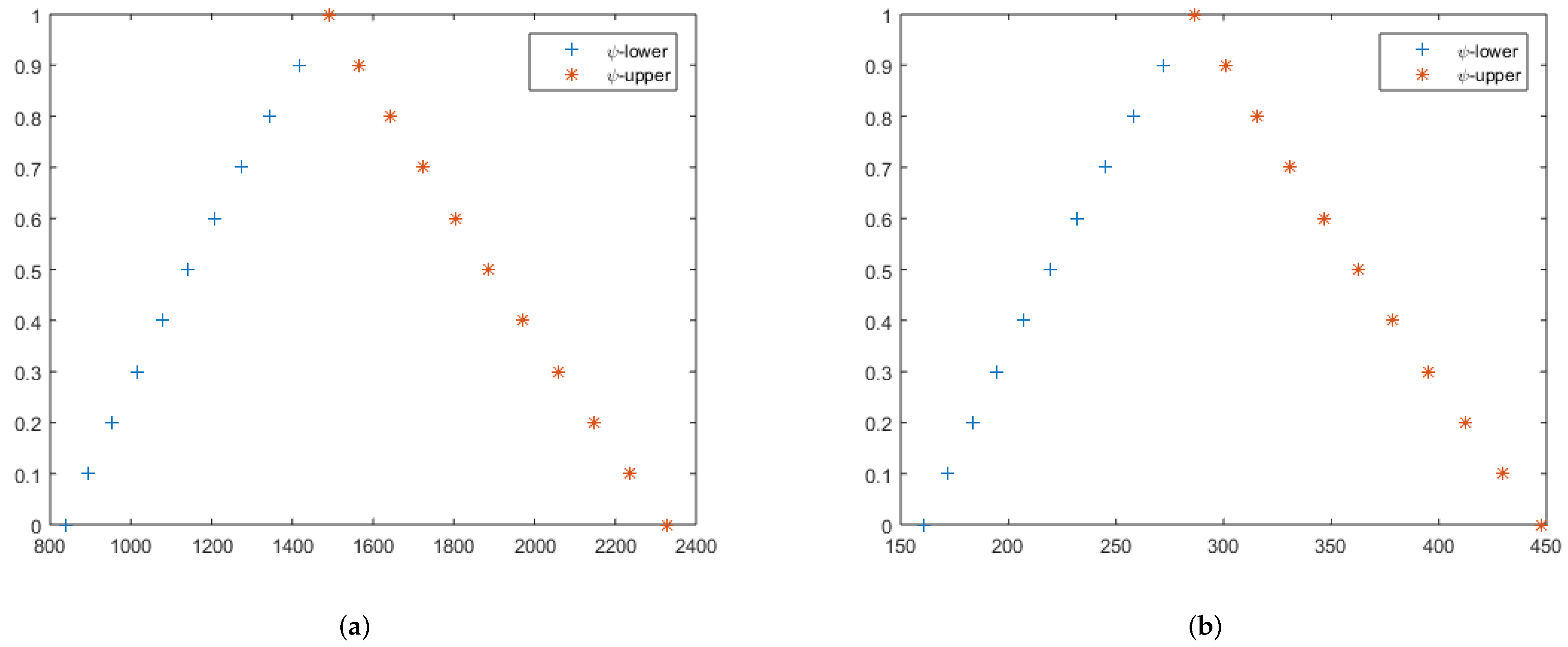
In Figure 1, we plot $2D$ graphs of the exact and approximation solutions for local fuzzy fractional differential equations (LFFDEs) on Cantor set. Figure 1a shows that for $\theta =45,\vartheta =2,\beta =1,n=2$, the LFFDEs become bounded and closed. In addition, the $\underline{\mathbb{W}}$ sign shows increasing functions and $\overline{\mathbb{W}}$ denotes decreasing functions on the $\varrho$-level set of $\mathbb{W}$. To reflect the concept of the $\varrho$-level set, Figure 1a illustrates that the $\varrho$-level set of LFFDEs is bounded and closed for $\theta =45$. Similarly, in Figure 1b, we can observe the same explanation of $\varrho$-level set closedness and boundedness for Example 1.

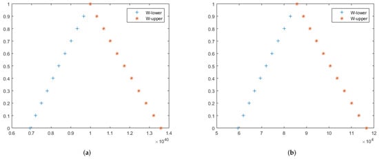
Figure 1. The exact and approximate lower and upper solutions of (46) at (a) $\theta =45,\vartheta =2,\beta =1,n=2$ (b) $\theta =45,\vartheta =2,\beta =0.5,n=2,$ respectively. Moreover, (a,b) are 2D figures for the exact and approximate solutions of local fuzzy fractional differential equations on Cantor of $\mathbb{W}(\vartheta ,\theta )$ in Example 1.

Example 2.

We consider the following local fuzzy fractional partial differential equation with a local fuzzy fractional differential operator:

$$\begin{array}{c}\hfill \frac{{\partial }^{4\beta }\mathbb{W}(\vartheta ,\theta )}{\partial {\theta }^{4\beta }}\ominus 2^{\beta }\odot \frac{{\partial }^{3\beta }\mathbb{W}(\vartheta ,\theta )}{\partial {\vartheta }^{3\beta }}=1,\theta >0,\vartheta \in R,0<\beta \le 1,\end{array}$$

(61)

with the initial conditions

$$\begin{array}{c}\hfill \begin{array}{cc}\hfill & \mathbb{W}(\vartheta ,0)=[{(3.5+0.5\varrho )}^n,{(4.5-0.5\varrho )}^n]\oplus E_{\beta }\left({\left(2\vartheta \right)}^{\beta }\right),\frac{{\partial }^{\beta }\mathbb{W}(\vartheta ,0)}{\partial {\theta }^{\beta }}=[{(3.5+0.5\varrho )}^n,{(4.5-0.5\varrho )}^n],\hfill \\ \hfill & \frac{{\partial }^{2\beta }\mathbb{W}(\vartheta ,0)}{\partial {\theta }^{2\beta }}=[{(3.5+0.5\varrho )}^n,{(4.5-0.5\varrho )}^n]\oplus \left(-2^{2\beta }{E}_{\beta }\left({\left(2\vartheta \right)}^{\beta }\right)\right),\frac{{\partial }^{3\beta }\mathbb{W}(\vartheta ,0)}{\partial {\theta }^{3\beta }}=[{(3.5+0.5\varrho )}^n,{(4.5-0.5\varrho )}^n],\hfill \end{array}\end{array}$$

(62)

where $n=1,2,3,\dots$

1. Local fuzzy fractional homotopy perturbation Sumudu transform method.

Using the LFFST for the LFFD formula in Equation (61), we obtain

$$\begin{array}{c}\hfill LFF{S}_{\beta }\left[\frac{{\partial }^{4\beta }\mathbb{W}(\vartheta ,\theta )}{\partial {\theta }^{4\beta }}\right]\ominus LFF{S}_{\beta }\left[2^{\beta }\odot \frac{{\partial }^{3\beta }\mathbb{W}(\vartheta ,\theta )}{\partial {\vartheta }^{3\beta }}\right]=1.\end{array}$$

(63)

Applying the LFFST for the LFD formula in Equation (63), we obtain

$$\begin{array}{cc}\hfill & \frac{1}{z^{4\beta }}\left[LFF{S}_{\beta }\left(\mathbb{W}(\vartheta ,\theta )\right)\ominus \mathbb{W}(\vartheta ,0)\ominus z^{\beta }{\mathbb{W}}^{\left(\beta \right)}(\vartheta ,0)\ominus z^{2\beta }{\mathbb{W}}^{2\beta }(\vartheta ,0)\ominus z^{\left(3\beta \right)}{\mathbb{W}}^{\left(3\beta \right)}(\vartheta ,0)\right]\hfill \\ \hfill & \ominus LFF{S}_{\beta }\left[2^{\beta }\odot \frac{{\partial }^{3\beta }\mathbb{W}(\vartheta ,\theta )}{\partial {\vartheta }^{3\beta }}\right]=1.\hfill \end{array}$$

(64)

After the rearrangement of the terms in Equation (64), we obtain

$$\begin{array}{cc}\hfill LFF{S}_{\beta }\left(\mathbb{W}(\vartheta ,\theta )\right)& =\mathbb{W}(\vartheta ,0)\oplus \mathbb{W}(\vartheta ,0)\oplus z^{\beta }{\mathbb{W}}^{\left(\beta \right)}(\vartheta ,0)\oplus z^{2\beta }{\mathbb{W}}^{2\beta }(\vartheta ,0)\oplus z^{\left(3\beta \right)}{\mathbb{W}}^{\left(3\beta \right)}(\vartheta ,0)\hfill \\ \hfill & \oplus z^{4\beta }LFF{S}_{\beta }\left[2^{\beta }\odot \frac{{\partial }^{3\beta }\mathbb{W}(\vartheta ,\theta )}{\partial {\vartheta }^{3\beta }}\right]\oplus z^{4\beta }.\hfill \end{array}$$

(65)

The initial conditions (62) can transform Equation (68) as

$$\begin{array}{cc}\hfill LFF{S}_{\beta }\left(\mathbb{W}(\vartheta ,\theta )\right)& =E_{\beta }\left({\left(2\vartheta \right)}^{\beta }\right)\ominus z^{2\beta }{2}^{2\beta }{E}_{\beta }\left({\left(2\vartheta \right)}^{\beta }\right)\oplus z^{4\beta }LFF{S}_{\beta }\left[2^{\beta }\odot \frac{{\partial }^{3\beta }\mathbb{W}(\vartheta ,\theta )}{\partial {\vartheta }^{3\beta }}\right]\oplus z^{4\beta }.\hfill \end{array}$$

(66)

Taking the inverse LFFST on Equation (66), we obtain

$$\begin{array}{cc}\hfill \mathbb{W}(\vartheta ,\theta )& =LFF{S}_{\beta }^{-1}\left(E_{\beta }\left({\left(2\vartheta \right)}^{\beta }\right)\right)\ominus LFF{S}_{\beta }^{-1}\left(z^{2\beta }{2}^{2\beta }{E}_{\beta }\left({\left(2\vartheta \right)}^{\beta }\right)\right)\hfill \\ \hfill & \oplus LFF{S}_{\beta }^{-1}\left[z^{4\beta }LFF{S}_{\beta }\left[2^{\beta }\odot \frac{{\partial }^{3\beta }\mathbb{W}(\vartheta ,\theta )}{\partial {\vartheta }^{3\beta }}\right]\right]\oplus LFF{S}_{\beta }^{-1}\left[z^{4\beta }\right].\hfill \end{array}$$

(67)

After simplification, Equation (67) yields

$$\begin{array}{cc}\hfill \mathbb{W}(\vartheta ,\theta )& =E_{\beta }\left({\left(2\vartheta \right)}^{\beta }\right)\left[1\ominus 2^{2\beta }\frac{{\theta }^{2\beta }}{\mathsf{\Gamma }(1+2\beta )}\right]\oplus \frac{{\theta }^{4\beta }}{\mathsf{\Gamma }(1+4\beta )}\oplus LFF{S}_{\beta }^{-1}\left[z^{4\beta }LFF{S}_{\beta }\left[2^{\beta }\frac{{\partial }^{3\beta }\mathbb{W}(\vartheta ,\theta )}{\partial {\vartheta }^{3\beta }}\right]\right].\hfill \end{array}$$

(68)

The LFFHPM proposes homotopy expression creation as

$$\begin{array}{cc}\hfill \sum _{n=0}^{\infty }{\rho }^{n\beta }{\mathbb{W}}_n(\vartheta ,\theta )& =[{(3.5+0.5\varrho )}^n,{(4.5-0.5\varrho )}^n]\oplus E_{\beta }\left({\left(2\vartheta \right)}^{\beta }\right)\left[1\ominus 2^{2\beta }\frac{{\theta }^{2\beta }}{\mathsf{\Gamma }(1+2\beta )}\right]\oplus \frac{{\theta }^{4\beta }}{\mathsf{\Gamma }(1+4\beta )}\hfill \\ \hfill & \ominus {\rho }^{\beta }LFF{S}_{\beta }^{-1}\left[z^{4\beta }{2}^{\beta }LFF{S}_{\beta }\left(\frac{{\partial }^{3\beta }\left\{{\sum }_{n=0}^{\infty }{\rho }^{n\beta }{\mathbb{W}}_n(\vartheta ,\theta )\right\}}{\partial {\vartheta }^{3\beta }}\right)\right].\hfill \end{array}$$

(69)

The following components for the series solution are calculated by comparing the powers of $\rho$ as

$$\begin{array}{c}\hfill \left\{\begin{array}{cc}\hfill & {\rho }^0:{\mathbb{W}}_0(\vartheta ,\theta )=[{(3.5+0.5\varrho )}^n,{(4.5-0.5\varrho )}^n]\oplus E_{\beta }\left({\left(2\vartheta \right)}^{\beta }\right)\left[1\ominus 2^{2\beta }\frac{{\theta }^{2\beta }}{\mathsf{\Gamma }(1+2\beta )}\right]\oplus \frac{{\theta }^{4\beta }}{\mathsf{\Gamma }(1+4\beta )},\hfill \\ \hfill & {\rho }^{1\beta }:{\mathbb{W}}_1(\vartheta ,\theta )=LFF{S}_{\beta }^{-1}\left[z^{4\beta }{2}^{\beta }LFF{S}_{\beta }\left(\frac{{\partial }^{3\beta }\left({\mathbb{W}}_0(\vartheta ,\theta )\right)}{\partial {\vartheta }^{3\beta }}\right)\right],\hfill \\ \hfill & {\rho }^{2\beta }:{\mathbb{W}}_2(\vartheta ,\theta )=LFF{S}_{\beta }^{-1}\left[z^{4\beta }{2}^{\beta }LFF{S}_{\beta }\left(\frac{{\partial }^{3\beta }\left({\mathbb{W}}_1(\vartheta ,\theta )\right)}{\partial {\vartheta }^{3\beta }}\right)\right],\hfill \\ \hfill & {\rho }^{3\beta }:{\mathbb{W}}_3(\vartheta ,\theta )=LFF{S}_{\beta }^{-1}\left[z^{4\beta }{2}^{\beta }LFF{S}_{\beta }\left(\frac{{\partial }^{3\beta }\left({\mathbb{W}}_2(\vartheta ,\theta )\right)}{\partial {\vartheta }^{3\beta }}\right)\right],\hfill \\ \hfill & ⋮.\hfill \end{array}\right.\end{array}$$

(70)

After simplification, we obtain

$$\begin{array}{c}\hfill \left\{\begin{array}{cc}\hfill & {\mathbb{W}}_0(\vartheta ,\theta )=[{(3.5+0.5\varrho )}^n,{(4.5-0.5\varrho )}^n]\oplus E_{\beta }\left({\left(2\vartheta \right)}^{\beta }\right)\left[1\ominus 2^{2\beta }\frac{{\theta }^{2\beta }}{\mathsf{\Gamma }(1+2\beta )}\right]\oplus \frac{{\theta }^{4\beta }}{\mathsf{\Gamma }(1+4\beta )},\hfill \\ \hfill & {\mathbb{W}}_1(\vartheta ,\theta )=[{(3.5+0.5\varrho )}^n,{(4.5-0.5\varrho )}^n]\oplus E_{\beta }\left({\left(2\vartheta \right)}^{\beta }\right)\left[2^{4\beta }\frac{{\theta }^{4\beta }}{\mathsf{\Gamma }(1+4\beta )}\ominus 2^{6\beta }\frac{{\theta }^{6\beta }}{\mathsf{\Gamma }(1+6\beta )}\right]\hfill \\ \hfill & {\mathbb{W}}_2(\vartheta ,\theta )=[{(3.5+0.5\varrho )}^n,{(4.5-0.5\varrho )}^n]\oplus E_{\beta }\left({\left(2\vartheta \right)}^{\beta }\right)\left[2^{8\beta }\frac{{\theta }^{4\beta }}{\mathsf{\Gamma }(1+8\beta )}\ominus 2^{10\beta }\frac{{\theta }^{10\beta }}{\mathsf{\Gamma }(1+10\beta )}\right]\hfill \\ \hfill & {\mathbb{W}}_3(\vartheta ,\theta )=[{(3.5+0.5\varrho )}^n,{(4.5-0.5\varrho )}^n]\oplus E_{\beta }\left({\left(2\vartheta \right)}^{\beta }\right)\left[2^{12\beta }\frac{{\theta }^{12\beta }}{\mathsf{\Gamma }(1+12\beta )}\ominus 2^{14\beta }\frac{{\theta }^{14\beta }}{\mathsf{\Gamma }(1+14\beta )}\right]\hfill \\ \hfill & ⋮.\hfill \end{array}\right.\end{array}$$

(71)

Hence, we can obtain the solutions of Equation (61) as follows:

$$\begin{array}{c}\hfill \begin{array}{cc}\hfill \mathbb{W}(\vartheta ,\theta )& =\sum _{n=0}^{\infty }{\mathbb{W}}_n(\vartheta ,\theta )\hfill \\ \hfill & =[{(3.5+0.5\varrho )}^n,{(4.5-0.5\varrho )}^n]\oplus \left[\frac{{\theta }^{4\beta }}{\mathsf{\Gamma }(1+4\beta )}\oplus E_{\beta }\left({\left(2\vartheta \right)}^{\beta }\right)\left(1\ominus 2^{2\beta }\frac{{\theta }^{2\beta }}{\mathsf{\Gamma }(1+2\beta )}\oplus 2^{4\beta }\frac{{\theta }^{4\beta }}{\mathsf{\Gamma }(1+4\beta )}\right.\right.\hfill \\ \hfill & \ominus 2^{6\beta }\frac{{\theta }^{6\beta }}{\mathsf{\Gamma }(1+6\beta )}\oplus 2^{8\beta }\frac{{\theta }^{8\beta }}{\mathsf{\Gamma }(1+8\beta )}\ominus 2^{10\beta }\frac{{\theta }^{10\beta }}{\mathsf{\Gamma }(1+10\beta )}\hfill \\ \hfill & \left.\left.\oplus 2^{12\beta }\frac{{\theta }^{12\beta }}{\mathsf{\Gamma }(1+12\beta )}\ominus 2^{14\beta }\frac{{\theta }^{14\beta }}{\mathsf{\Gamma }(1+14\beta )}\oplus \cdots \right)\right]\hfill \\ \hfill & =[{(3.5+0.5\varrho )}^n,{(4.5-0.5\varrho )}^n]\oplus \left[\frac{{\theta }^{4\beta }}{\mathsf{\Gamma }(1+4\beta )}\oplus E_{\beta }\left({\left(2\vartheta \right)}^{\beta }\right)\left(1\ominus \frac{{\left(2\theta \right)}^{2\beta }}{\mathsf{\Gamma }(1+2\beta )}\oplus \frac{{\left(2\theta \right)}^{4\beta }}{\mathsf{\Gamma }(1+4\beta )}\ominus \frac{{\left(2\theta \right)}^{6\beta }}{\mathsf{\Gamma }(1+6\beta )}\right.\right.\hfill \\ \hfill & \oplus \frac{{\left(2\theta \right)}^{8\beta }}{\mathsf{\Gamma }(1+8\beta )}\ominus \frac{{\left(2\theta \right)}^{10\beta }}{\mathsf{\Gamma }(1+10\beta )}\oplus \frac{{\left(2\theta \right)}^{12\beta }}{\mathsf{\Gamma }(1+12\beta )}\ominus \frac{{\left(2\theta \right)}^{14\beta }}{\mathsf{\Gamma }(1+14\beta )}\hfill \\ \hfill & \left.\left.\oplus \cdots \oplus {(-1)}^n\frac{{\left(2\theta \right)}^{2n\beta }}{\mathsf{\Gamma }(1+2n\beta )}\oplus \cdots \right)\right]\hfill \\ \hfill & =[{(3.5+0.5\varrho )}^n,{(4.5-0.5\varrho )}^n]\oplus \left[\frac{{\left(\theta \right)}^{4\beta }}{\mathsf{\Gamma }(1+4\beta )}\oplus E_{\beta }\left({\left(2\vartheta \right)}^{\beta }\right)\left(\sum _{n=0}^{\infty }{(-1)}^n\frac{{\left(2\theta \right)}^{2n\beta }}{\mathsf{\Gamma }(1+2n\beta )}\right)\right]\hfill \end{array}\end{array}$$

(72)

or

$$\begin{array}{c}\hfill \mathbb{W}(\vartheta ,\theta )=[{(3.5+0.5\varrho )}^n,{(4.5-0.5\varrho )}^n]\oplus \left[\frac{{\theta }^{4\beta }}{\mathsf{\Gamma }(1+4\beta )}\oplus E_{\beta }\left({\left(2\vartheta \right)}^{\beta }\right)\cos \left({\left(2\vartheta \right)}^{\beta }\right)\right].\end{array}$$

(73)

2. Local fuzzy fractional Sumudu decomposition method.

Utilizing equations (39) and (61), we can obtain the subsequent mathematical expression

$$\begin{array}{c}\hfill \begin{array}{cc}\hfill {\mathbb{U}}_0(\vartheta ,\theta )& =[{(3.5+0.5\varrho )}^n,{(4.5-0.5\varrho )}^n]\oplus E_{\beta }{\left(2\vartheta \right)}^{\beta }\ominus 2^{2\beta }{E}_{\beta }\left({\left(2\vartheta \right)}^{\beta }\right)\frac{{\theta }^{2\beta }}{\mathsf{\Gamma }(1+2\vartheta )}\oplus \frac{{\theta }^{4\beta }}{\mathsf{\Gamma }(1+4\beta )}\hfill \\ \hfill {\mathbb{U}}_n(\vartheta ,\theta )& =LFF{S}_v^{-1}\left(u^{4\beta }\left(LFF{S}_{\beta }\left[2^{\beta }\frac{{\partial }^{3\beta }{\mathbb{U}}_{n-1}(\vartheta ,\theta )}{\partial {\vartheta }^{3\beta }}\right]\right)\right),n\ge 1.\hfill \end{array}\end{array}$$

(74)

Applying the formula (74), successive approximations are obtained as follows:

$$\begin{array}{c}\hfill \begin{array}{cc}\hfill {\mathbb{U}}_0(\vartheta ,\theta )& =[{(3.5+0.5\varrho )}^n,{(4.5-0.5\varrho )}^n]\oplus \left[E_{\beta }\left({\left(2\vartheta \right)}^{\beta }\right)\left(1\ominus 2^{2\beta }\frac{{\theta }^{2\beta }}{\mathsf{\Gamma }(1+2\beta )}\right)\oplus \frac{{\theta }^{4\beta }}{\mathsf{\Gamma }(1+4\beta )}\right],\hfill \\ \hfill {\mathbb{U}}_1(\vartheta ,\theta )& =LFF{S}_{\beta }^{-1}\left(u^{4\beta }\left(LFF{S}_{\beta }\left[2^{\beta }\frac{{\partial }^{3\beta }{\mathbb{U}}_0(\vartheta ,\theta )}{\partial {\vartheta }^{3\beta }}\right]\right)\right),\hfill \\ \hfill {\mathbb{U}}_2(\vartheta ,\theta )& =LFF{S}_{\beta }^{-1}\left(u^{4\beta }\left(LFF{S}_{\beta }\left[2^{\beta }\frac{{\partial }^{3\beta }{\mathbb{U}}_1(\vartheta ,\theta )}{\partial {\vartheta }^{3\beta }}\right]\right)\right),\hfill \\ \hfill {\mathbb{U}}_3(\vartheta ,\theta )& =LFF{S}_{\beta }^{-1}\left(u^{4\beta }\left(LFF{S}_{\beta }\left[2^{\beta }\frac{{\partial }^{3\beta }{\mathbb{U}}_2(\vartheta ,\theta )}{\partial {\vartheta }^{3\beta }}\right]\right)\right),\hfill \\ \hfill & ⋮.\hfill \end{array}\end{array}$$

(75)

The first terms of LFFSDM have the following form:

$$\begin{array}{c}\hfill \begin{array}{cc}\hfill {\mathbb{W}}_0(\vartheta ,\theta )& =[{(3.5+0.5\varrho )}^n,{(4.5-0.5\varrho )}^n]\oplus \left[E_{\beta }\left({\left(2\vartheta \right)}^{\beta }\right)\left(1\ominus 2^{2\beta }\frac{{\theta }^{2\beta }}{\mathsf{\Gamma }(1+2\beta )}\right)\oplus \frac{{\theta }^{4\beta }}{\mathsf{\Gamma }(1+4\beta )}\right]\hfill \\ \hfill {\mathbb{W}}_1(\vartheta ,\theta )& =[{(3.5+0.5\varrho )}^n,{(4.5-0.5\varrho )}^n]\oplus \left[E_{\beta }\left({\left(2\vartheta \right)}^{\beta }\right)\left(2^{4\beta }\frac{{\theta }^{4\beta }}{\mathsf{\Gamma }(1+2\beta )}\ominus 2^{6\beta }\frac{{\theta }^{6\beta }}{\mathsf{\Gamma }(1+6\beta )}\right)\right]\hfill \\ \hfill {\mathbb{W}}_2(\vartheta ,\theta )& =[{(3.5+0.5\varrho )}^n,{(4.5-0.5\varrho )}^n]\oplus \left[E_{\beta }\left({\left(2\vartheta \right)}^{\beta }\right)\left(2^{8\beta }\frac{{\theta }^{8\beta }}{\mathsf{\Gamma }(1+8\beta )}\ominus 2^{10\beta }\frac{{\theta }^{10\beta }}{\mathsf{\Gamma }(1+10\beta )}\right)\right]\hfill \\ \hfill {\mathbb{W}}_3(\vartheta ,\theta )& =[{(3.5+0.5\varrho )}^n,{(4.5-0.5\varrho )}^n]\oplus \left[E_{\beta }\left({\left(2\vartheta \right)}^{\beta }\right)\left(2^{12\beta }\frac{{\theta }^{12\beta }}{\mathsf{\Gamma }(1+12\beta )}\ominus 2^{14\beta }\frac{{\theta }^{14\beta }}{\mathsf{\Gamma }(1+14\beta )}\right)\right]\hfill \\ \hfill & ⋮.\hfill \end{array}\end{array}$$

(76)

The local fractional series form can be expressed as

$$\begin{array}{cc}\hfill \mathbb{W}(\vartheta ,\theta )& =[{(3.5+0.5\varrho )}^n,{(4.5-0.5\varrho )}^n]\oplus \left[\frac{{\theta }^{4\beta }}{\mathsf{\Gamma }(1+4\beta )}+E_{\beta }\left({\left(2\vartheta \right)}^{\beta }\right)\left(1\ominus \frac{{\left(2\theta \right)}^{2\beta }}{\mathsf{\Gamma }(1+2\beta )}\oplus \frac{{\left(2\theta \right)}^{4\beta }}{\mathsf{\Gamma }(1+4\beta )}\ominus \frac{{\left(2\theta \right)}^{6\beta }}{\mathsf{\Gamma }(1+6\beta )}\right.\right.\hfill \\ \hfill & \left.\left.\oplus \frac{{\left(2\theta \right)}^{8\beta }}{\mathsf{\Gamma }(1+8\beta )}\ominus \frac{{\left(2\theta \right)}^{10\beta }}{\mathsf{\Gamma }(1+10\beta )}\oplus \cdots \oplus {(-1)}^n\frac{{\left(2\theta \right)}^{2n\beta }}{\mathsf{\Gamma }(1+2n\beta )}\oplus \cdots \right)\right].\hfill \end{array}$$

(77)

Therefore, the exact solution of (61), as determined by LFFSDM, is given by

$$\begin{array}{cc}\hfill \mathbb{W}(\vartheta ,\theta )& =[{(3.5+0.5\varrho )}^n,{(4.5-0.5\varrho )}^n]\oplus \left[\frac{{\theta }^{4\beta }}{\mathsf{\Gamma }(1+4\beta )}\oplus E_{\beta }\left({\left(2\vartheta \right)}^{\beta }\right)\sum _{n=0}^{\infty }{(-1)}^n\frac{{\left(2\theta \right)}^{2n\beta }}{\mathsf{\Gamma }(1+2n\beta )}\right].\hfill \end{array}$$

Therefore, the exact solution can be achieved as

$$\begin{array}{cc}\hfill \mathbb{W}(\vartheta ,\theta )& =[{(3.5+0.5\varrho )}^n,{(4.5-0.5\varrho )}^n]\oplus \left[\frac{{\theta }^{4\beta }}{\mathsf{\Gamma }(1+4\beta )}\oplus E_{\beta }\left({\left(2\vartheta \right)}^{\beta }\right)\cos \left({\left(2\theta \right)}^{\beta }\right)\right].\hfill \end{array}$$

(78)

Table 1 shows the error term between exact and approximate solutions of Example 2 for $\varrho \in [0,1]$.

Table 1. For the absolute error between exact solutions (E-S) at $\beta =1$ and approximate solutions (A-S) at $\beta =0.5$.

$\mathit{\varrho }$	Lower E-S	Lower A-S	Lower Error	Upper E-S	Upper A-S	Upper Error
0	33,369	482.42	32,887	33370	483.42	32,887
0.1	33,369	482.47	32,887	33,370	483.37	32,887
0.2	33,369	482.52	32,887	33,370	483.32	32,887
0.3	33,369	482.57	32,887	33,370	483.27	32,887
0.4	33,369	482.62	32,887	33,370	483.22	32,887
0.5	33,370	482.67	32,887	33,370	483.17	32,887
0.6	33,370	482.72	32,887	33,370	483.12	32,887
0.7	33,370	482.77	32,887	33,370	483.07	32,887
0.8	33,370	482.82	32,887	33,370	483.02	32,887
0.9	33,370	482.87	32,887	33,370	482.97	32,887
1	33,370	482.92	32,887	33,370	482.92	32,887

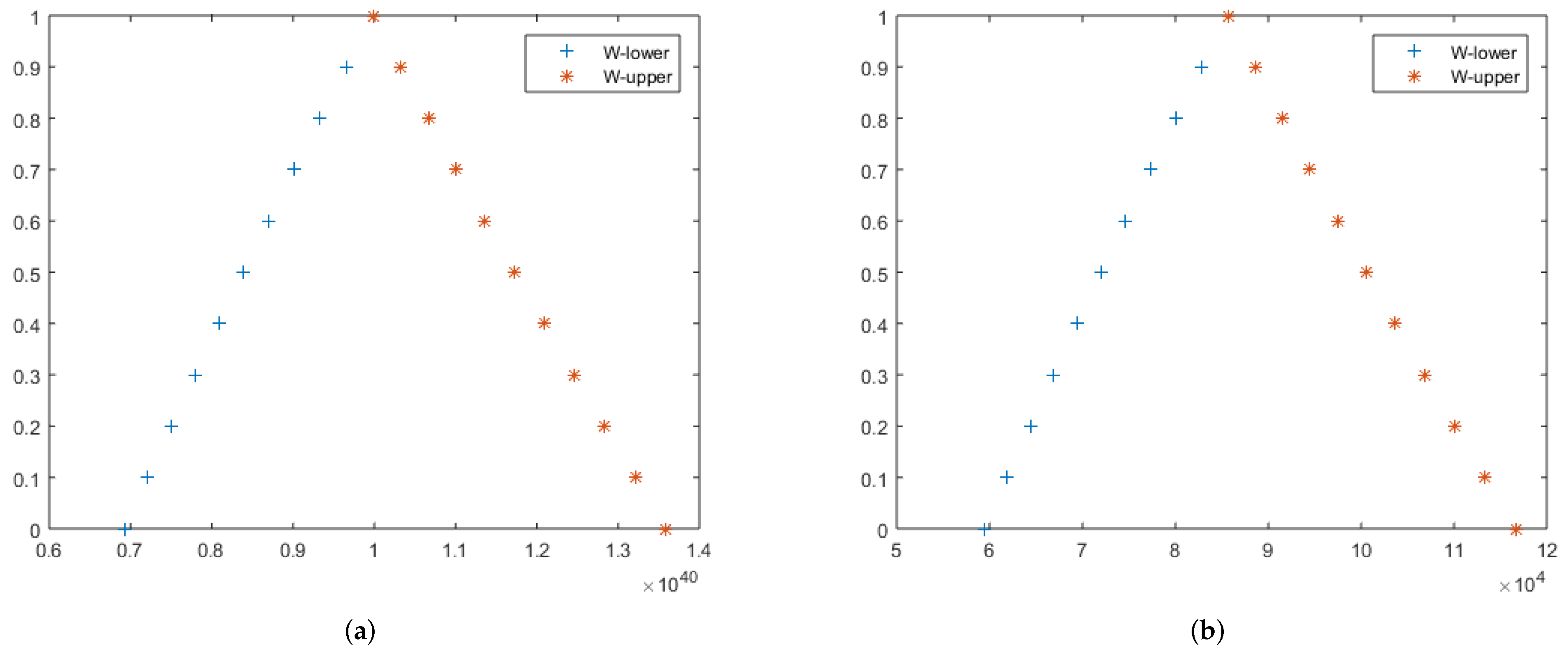
In Figure 2, we plot $2D$ graphs of the exact and approximation solutions for local fuzzy fractional partial differential equations with local fuzzy fractional differential operators. Figure 2a shows that for $\theta =30,\vartheta =3$, $\beta =1,n=1$, the LFFPDEs become bounded and closed. In addition, the $\underline{\mathbb{W}}$ sign shows increasing functions and $\overline{\mathbb{W}}$ denotes decreasing functions on the $\varrho$-level set of $\mathbb{W}$. To reflect the concept of the $\varrho$-level set, Figure 2a illustrates that the $\varrho$-level set of LFFPDEs is bounded and closed for $\theta =30$. Similarly, in Figure 2b, we can observe the same explanation of $\varrho$-level set closedness and boundedness for Example 2.

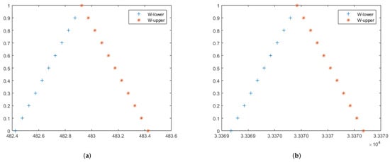
Figure 2. The exact and approximate lower and upper solutions of (61) at (a) $\theta =30,\vartheta =3,\beta =1,n=1$ (b) $\theta =30,\vartheta =3,\beta =0.5,n=1.$ Further, (a,b) are 2D figures for the exact and approximate solutions of local fuzzy fractional partial differential equations with local fuzzy fractional differential operators of $\mathbb{W}(\vartheta ,\theta )$ in Example 2.

Example 3.

We consider the following local fuzzy fractional partial differential equation

$$\begin{array}{c}\hfill \frac{{\partial }^{2\beta }\mathbb{W}(\vartheta ,\theta )}{\partial {\theta }^{2\beta }}\oplus \frac{{\partial }^{2\beta }\mathbb{W}(\vartheta ,\theta )}{\partial {\vartheta }^{2\beta }}\ominus 3\odot \mathbb{W}(\vartheta ,\theta )=0,\theta >0,\vartheta \in R,0<\beta \le 1,\end{array}$$

(79)

with the initial condition

$$\begin{array}{c}\hfill \mathbb{W}(\vartheta ,0)=\left[{(5.5+0.5\varrho )}^n,{(6.5-0.5\varrho )}^n\right]\oplus {\sin }_{\beta }\left({\vartheta }^{\beta }\right),\frac{{\partial }^{\beta }\mathbb{W}(\vartheta ,0)}{\partial {\theta }^{\beta }}=\left[{(5.5+0.5\varrho )}^n,{(6.5-0.5\varrho )}^n\right]\oplus 2{\sin }_{\beta }\left({\vartheta }^{\beta }\right)\end{array}$$

(80)

where $n=1,2,3,\dots$

1. Local fuzzy fractional homotopy perturbation Sumudu transform method

Applying the LFFST of Equation (79), we obtain the following:

$$\begin{array}{c}\hfill LFF{S}_{\beta }\left[\frac{{\partial }^{2\beta }\mathbb{W}(\vartheta ,\theta )}{\partial {\theta }^{2\beta }}\right]\oplus LFF{S}_{\beta }\left[\frac{{\partial }^{2\beta }\mathbb{W}(\vartheta ,\theta )}{\partial {\vartheta }^{2\beta }}\right]=3LFF{S}_{\beta }\left(\mathbb{W}(\vartheta ,\theta )\right).\end{array}$$

(81)

Taking the formula of LFFST for the LFFDs in Equation (81), we obtain

$$\begin{array}{c}\hfill LFF{S}_{\beta }\left[\frac{{\partial }^{2\beta }\mathbb{W}(\vartheta ,\theta )}{\partial {\vartheta }^{2\beta }}\right]\oplus \frac{1}{z^{2\beta }}\left[LFF{S}_{\beta }\left(\mathbb{W}(\vartheta ,\theta )\right)\ominus \mathbb{W}(\vartheta ,0)\ominus z^{\beta }{\mathbb{W}}^{\left(\beta \right)}(\vartheta ,0)\right]=3LFF{S}_{\beta }\left(\mathbb{W}(\vartheta ,\theta )\right).\end{array}$$

(82)

Rearranging the terms given in Equation (82) yields

$$\begin{array}{c}\hfill LFF{S}_{\beta }\left(\mathbb{W}(\vartheta ,\theta )\right)=\mathbb{W}(\vartheta ,0)\oplus z^{\beta }{\mathbb{W}}^{\left(\beta \right)}(\vartheta ,0)\oplus 3z^{2\beta }LFF{S}_{\beta }\left(\mathbb{W}(\vartheta ,\theta )\right)\ominus z^{2\beta }LFF{S}_{\beta }\left[\frac{{\partial }^{2\beta }\mathbb{W}(\vartheta ,\theta )}{\partial {\vartheta }^{2\beta }}\right].\end{array}$$

(83)

Moreover, Equation (83) is simplified for the initial condition (80) in the following manner:

$$\begin{array}{cc}\hfill LFF{S}_{\beta }\left(\mathbb{W}(\vartheta ,\theta )\right)& =\left[{(5.5+0.5\varrho )}^n,{(6.5-0.5\varrho )}^n\right]\oplus \left[{\sin }_{\beta }\left({\vartheta }^{\beta }\right)\ominus 2z^{\beta }{\sin }_{\beta }\left({\vartheta }^{\beta }\right)\oplus 3z^{2\beta }LFF{S}_{\beta }\left(\mathbb{W}(\vartheta ,\theta )\right)\right.\hfill \\ \hfill & \left.\ominus z^{2\beta }LFF{S}_{\beta }\left[\frac{{\partial }^{2\beta }\mathbb{W}(\vartheta ,\theta )}{\partial {\vartheta }^{2\beta }}\right]\right].\hfill \end{array}$$

(84)

We apply the inverse of LFFST on Equation (83) to obtain

$$\begin{array}{cc}\hfill \left(\mathbb{W}(\vartheta ,\theta )\right)& =\left[{(5.5+0.5\varrho )}^n,{(6.5-0.5\varrho )}^n\right]\oplus \left[{\sin }_{\beta }\left({\vartheta }^{\beta }\right)\ominus 2LFF{S}_{\beta }^{-1}\left(z^{\beta }{\sin }_{\beta }\left({\vartheta }^{\beta }\right)\right)\oplus 3LFF{S}_{\beta }^{-1}\left[z^{2\beta }LFF{S}_{\beta }\left(\mathbb{W}(\vartheta ,\theta )\right)\right]\right.\hfill \\ \hfill & \left.\ominus LFF{S}_{\beta }^{-1}\left[z^{2\beta }LFF{S}_{\beta }\left[\frac{{\partial }^{2\beta }\mathbb{W}(\vartheta ,\theta )}{\partial {\vartheta }^{2\beta }}\right]\right]\right].\hfill \end{array}$$

(85)

The homotopy expression can be established using the fundamental method of LFFHPM:

$$\begin{array}{cc}\hfill \sum _{n=0}^{\infty }{\rho }^{n\beta }{\mathbb{W}}_n(\vartheta ,\theta )& =\left[{(5.5+0.5\varrho )}^n,{(6.5-0.5\varrho )}^n\right]\oplus \left[{\sin }_{\beta }\left({\vartheta }^{\beta }\right)\oplus 2{\sin }_{\beta }\left({\vartheta }^{\beta }\right)\frac{{\theta }^{\beta }}{\mathsf{\Gamma }(1+\beta )}\right.\hfill \\ \hfill & \oplus 3{\rho }^{\beta }LFF{S}_{\beta }^{-1}\left[z^{2\beta }LFF{S}_{\beta }\left(\sum _{n=0}^{\infty }{\rho }^{n\beta }{\mathbb{W}}_n(\vartheta ,\theta )\right)\right]\hfill \\ \hfill & \left.\ominus {\rho }^{\beta }LFF{S}_{\beta }^{-1}\left[z^{2\beta }LFF{S}_{\beta }\left(\frac{{\partial }^{2\beta \left\{{\sum }_{n=0}^{\infty }{\rho }^{n\beta }{\mathbb{W}}_n(\vartheta ,\theta )\right\}}}{\partial {\vartheta }^{2\beta }}\right)\right]\right].\hfill \end{array}$$

(86)

The comparison of the similar powers of $\rho$ yields the subsequent components of the series solution:

$$\begin{array}{c}\hfill \begin{array}{cc}\hfill {\rho }^0:{\mathbb{W}}_0(\vartheta ,\theta )& =\left[{(5.5+0.5\varrho )}^n,{(6.5-0.5\varrho )}^n\right]\oplus \left[{\sin }_{\beta }\left({\vartheta }^{\beta }\right)\oplus 2{\sin }_{\beta }\left({\vartheta }^{\beta }\right)\frac{{\theta }^{\beta }}{\mathsf{\Gamma }(1+\beta )}\right]\hfill \\ \hfill {\rho }^{1\beta }:{\mathbb{W}}_1(\vartheta ,\theta )& =\left[{(5.5+0.5\varrho )}^n,{(6.5-0.5\varrho )}^n\right]\oplus \left[3LFF{S}_{\beta }^{-1}\left[z^{2\beta }LFF{S}_{\beta }\left({\mathbb{W}}_0(\vartheta ,\theta )\right)\right]\right.\hfill \\ \hfill & \left.\ominus LFF{S}_{\beta }^{-1}\left[z^{2\beta }LFF{S}_{\beta }\left[\frac{{\partial }^{2\beta }{\mathbb{W}}_0(\vartheta ,\theta )}{\partial {\vartheta }^{2\beta }}\right]\right]\right]\hfill \\ \hfill {\rho }^{2\beta }:{\mathbb{W}}_2(\vartheta ,\theta )& =\left[{(5.5+0.5\varrho )}^n,{(6.5-0.5\varrho )}^n\right]\oplus \left[3LFF{S}_{\beta }^{-1}\left[z^{2\beta }LFF{S}_{\beta }\left({\mathbb{W}}_1(\vartheta ,\theta )\right)\right]\right.\hfill \\ \hfill & \left.\ominus LFF{S}_{\beta }^{-1}\left[z^{2\beta }LFF{S}_{\beta }\left[\frac{{\partial }^{2\beta }{\mathbb{W}}_1(\vartheta ,\theta )}{\partial {\vartheta }^{2\beta }}\right]\right]\right]\hfill \\ \hfill & ⋮\hfill \\ \hfill {\rho }^{n\beta }:{\mathbb{W}}_n(\vartheta ,\theta )& =\left[{(5.5+0.5\varrho )}^n,{(6.5-0.5\varrho )}^n\right]\oplus \left[3LFF{S}_{\beta }^{-1}\left[z^{2\beta }LFF{S}_{\beta }\left({\mathbb{W}}_{n-1}(\vartheta ,\theta )\right)\right]\right.\hfill \\ \hfill & \left.\ominus LFF{S}_{\beta }^{-1}\left[z^{2\beta }LFF{S}_{\beta }\left[\frac{{\partial }^{2\beta }{\mathbb{W}}_{n-1}(\vartheta ,\theta )}{\partial {\vartheta }^{2\beta }}\right]\right]\right].\hfill \end{array}\end{array}$$

Following the reduction technique, we have

$$\begin{array}{c}\hfill \begin{array}{cc}\hfill {\mathbb{W}}_0(\vartheta ,\theta )& =\left[{(5.5+0.5\varrho )}^n,{(6.5-0.5\varrho )}^n\right]\oplus \left[{\sin }_{\beta }\left({\vartheta }^{\beta }\right)\oplus 2{\sin }_{\beta }\left({\vartheta }^{\beta }\right)\frac{{\theta }^{\beta }}{\mathsf{\Gamma }(1+\beta )}\right]\hfill \\ \hfill {\mathbb{W}}_1(\vartheta ,\theta )& =\left[{(5.5+0.5\varrho )}^n,{(6.5-0.5\varrho )}^n\right]\oplus \left[{\sin }_{\beta }\left({\vartheta }^{\beta }\right)\left[\frac{4{\theta }^{2\beta }}{\mathsf{\Gamma }(1+2\beta )}\oplus \frac{8{\theta }^{3\beta }}{\mathsf{\Gamma }(1+3\beta )}\right]\right]\hfill \\ \hfill {\mathbb{W}}_2(\vartheta ,\theta )& =\left[{(5.5+0.5\varrho )}^n,{(6.5-0.5\varrho )}^n\right]\oplus \left[{\sin }_{\beta }\left({\vartheta }^{\beta }\right)\left[\frac{16{\theta }^{4\beta }}{\mathsf{\Gamma }(1+4\beta )}\oplus \frac{32{\theta }^{5\beta }}{\mathsf{\Gamma }(1+5\beta )}\right]\right]\hfill \\ \hfill {\mathbb{W}}_3(\vartheta ,\theta )& =\left[{(5.5+0.5\varrho )}^n,{(6.5-0.5\varrho )}^n\right]\oplus \left[{\sin }_{\beta }\left({\vartheta }^{\beta }\right)\left[\frac{64{\theta }^{6\beta }}{\mathsf{\Gamma }(1+6\beta )}\oplus \frac{128{\theta }^{7\beta }}{\mathsf{\Gamma }(1+7\beta )}\right]\right]\hfill \\ \hfill & ⋮\hfill \\ \hfill {\mathbb{W}}_n(\vartheta ,\theta )& =\left[{(5.5+0.5\varrho )}^n,{(6.5-0.5\varrho )}^n\right]\oplus \left[{\sin }_{\beta }\left({\vartheta }^{\beta }\right)\left[\frac{{\left(2{\theta }^{\beta }\right)}^{2n}}{\mathsf{\Gamma }(1+2n\beta )}\oplus \frac{{\left(2{\theta }^{\beta }\right)}^{(2n+1)}}{\mathsf{\Gamma }(1+(2n+1\left)\beta \right)}\right]\right].\hfill \end{array}\end{array}$$

(87)

Therefore, the solution to Equation (79) is expressed as

$$\begin{array}{c}\hfill \begin{array}{cc}\hfill \mathbb{W}(\vartheta ,\theta )& =\left[{(5.5+0.5\varrho )}^n,{(6.5-0.5\varrho )}^n\right]\oplus \left[{\sin }_{\beta }\left({\vartheta }^{\beta }\right)\left(1\oplus \frac{2{\theta }^{\beta }}{\mathsf{\Gamma }(1+\beta )}\oplus \frac{4{\theta }^{2\beta }}{\mathsf{\Gamma }(1+2\beta )}\oplus \frac{8{\theta }^{3\beta }}{\mathsf{\Gamma }(1+3\beta )}\right.\right.\hfill \\ \hfill & \left.\left.\oplus \frac{16{\theta }^{4\beta }}{\mathsf{\Gamma }(1+4\beta )}\oplus \frac{32{\theta }^{5\beta }}{\mathsf{\Gamma }(1+5\beta )}\oplus \cdots \oplus \frac{{\left(2{\theta }^{\beta }\right)}^n}{\mathsf{\Gamma }(1+n\beta )}\right)\right].\hfill \end{array}\end{array}$$

Thus, we achieve our desired solution as

$$\begin{array}{cc}\hfill \mathbb{W}(\vartheta ,\theta )& =\left[{(5.5+0.5\varrho )}^n,{(6.5-0.5\varrho )}^n\right]\oplus \left({\sin }_{\beta }\left({\vartheta }^{\beta }\right)E_{\beta }\left(2{\theta }^{\beta }\right)\right).\hfill \end{array}$$

(88)

2. Local fuzzy fractional Sumudu variational iteration method

The formula for consecutive approximations given in (45) and (79) is

$$\begin{array}{cc}\hfill {\mathbb{W}}_{n+1}(\vartheta ,\theta )& ={\mathbb{W}}_n(\vartheta ,\theta ){\ominus }_0{I}_t^{\left(\beta \right)}\left[\frac{{\partial }^{2\beta }{\mathbb{W}}_n(\vartheta ,\theta )}{\partial {\theta }^{2\beta }}\ominus \frac{{\partial }^{\beta }\mathbb{W}(\vartheta ,0)}{\partial {\theta }^{\beta }}\right.\hfill \\ \hfill & \left.\oplus S_{\beta }^{-1}\left(u^{2\beta }{S}_{\beta }\left[\frac{{\partial }^{2\beta }{\mathbb{W}}_n(\vartheta ,\theta )}{\partial {\vartheta }^{2\beta }}\ominus 3{\mathbb{W}}_n(\vartheta ,\theta )\right]\right)\right].\hfill \end{array}$$

(89)

The initial conditions (80), the successive formula (89), and the result are as follows:

$$\begin{array}{c}\hfill \begin{array}{cc}\hfill {\mathbb{W}}_0(\vartheta ,\theta )& =\left[{(5.5+0.5\varrho )}^n,{(6.5-0.5\varrho )}^n\right]\oplus \left[{\sin }_{\beta }\left({\vartheta }^{\beta }\right)+2{\sin }_{\beta }\left({\vartheta }^{\beta }\right)\frac{{\theta }^{\beta }}{\mathsf{\Gamma }(1+\beta )}\right]\hfill \\ \hfill {\mathbb{W}}_1(\vartheta ,\theta )& ={\mathbb{W}}_0(\vartheta ,\theta ){\ominus }_0{I}_{\theta }^{\left(\beta \right)}\left[\frac{{\partial }^{2\beta }{\mathbb{W}}_0(\vartheta ,\theta )}{\partial {\theta }^{2\beta }}\ominus \frac{{\partial }^{\beta }W(\vartheta ,0)}{\partial {\theta }^{\beta }}\right.\hfill \\ \hfill & \left.\oplus S_{\beta }^{-1}\left(u^{2\beta }{S}_{\beta }\left[\frac{{\partial }^{2\beta }{\mathbb{W}}_0(\vartheta ,\theta )}{\partial {\vartheta }^{2\beta }}\ominus 3{\mathbb{W}}_0(\vartheta ,\theta )\right]\right)\right]\hfill \\ \hfill {\mathbb{W}}_2(\vartheta ,\theta )& ={\mathbb{W}}_1(\vartheta ,\theta ){\ominus }_0{I}_{\theta }^{\left(\beta \right)}\left[\frac{{\partial }^{2\beta }{\mathbb{W}}_1(\vartheta ,\theta )}{\partial {\theta }^{2\beta }}\ominus \frac{{\partial }^{\beta }\mathbb{W}(\vartheta ,0)}{\partial {\theta }^{\beta }}\right.\hfill \\ \hfill & \left.\oplus S_{\beta }^{-1}\left(u^{2\beta }{S}_{\beta }\left[\frac{{\partial }^{2\beta }{\mathbb{W}}_1(\vartheta ,\theta )}{\partial {\vartheta }^{2\beta }}\ominus 3{\mathbb{W}}_1(\vartheta ,\theta )\right]\right)\right]\hfill \\ \hfill & ⋮.\hfill \end{array}\end{array}$$

(90)

According to the above equations, the first of LFFSVIM can be obtained as

$$\begin{array}{c}\hfill \begin{array}{cc}\hfill {\mathbb{W}}_0(\vartheta ,\theta )& =\left[{(5.5+0.5\varrho )}^n,{(6.5-0.5\varrho )}^n\right]\oplus {\sin }_{\beta }\left({\vartheta }^{\beta }\right)\left[1\oplus \frac{2{\theta }^{\beta }}{\mathsf{\Gamma }(1+\beta )}\right],\hfill \\ \hfill {\mathbb{W}}_1(\vartheta ,\theta )& =\left[{(5.5+0.5\varrho )}^n,{(6.5-0.5\varrho )}^n\right]\oplus {\sin }_{\beta }\left({\vartheta }^{\beta }\right)\left[1\oplus \frac{2{\theta }^{\beta }}{\mathsf{\Gamma }(1+\beta )}\oplus \frac{4{\theta }^{\beta }}{\mathsf{\Gamma }(1+2\beta )}\oplus \frac{8{\theta }^{\beta }}{\mathsf{\Gamma }(1+3\beta )}\right],\hfill \\ \hfill {\mathbb{W}}_2(\vartheta ,\theta )& =\left[{(5.5+0.5\varrho )}^n,{(6.5-0.5\varrho )}^n\right]\oplus {\sin }_{\beta }\left({\vartheta }^{\beta }\right)\left[1\oplus \frac{2{\theta }^{\beta }}{\mathsf{\Gamma }(1+\beta )}\oplus \frac{4{\theta }^{\beta }}{\mathsf{\Gamma }(1+2\beta )}\oplus \frac{8{\theta }^{\beta }}{\mathsf{\Gamma }(1+3\beta )}\oplus \frac{16{\theta }^{4\beta }}{\mathsf{\Gamma }(1+4\beta )}\oplus \frac{32{\theta }^{5\beta }}{\mathsf{\Gamma }(1+5\beta )}\right]\hfill \\ \hfill {\mathbb{W}}_3(\vartheta ,\theta )& =\left[{(5.5+0.5\varrho )}^n,{(6.5-0.5\varrho )}^n\right]\oplus {\sin }_{\beta }\left({\vartheta }^{\beta }\right)\left[1\oplus \frac{2{\theta }^{\beta }}{\mathsf{\Gamma }(1+\beta )}\oplus \frac{4{\theta }^{\beta }}{\mathsf{\Gamma }(1+2\beta )}\oplus \frac{8{\theta }^{\beta }}{\mathsf{\Gamma }(1+3\beta )}\oplus \frac{16{\theta }^{4\beta }}{\mathsf{\Gamma }(1+4\beta )}\right.\hfill \\ \hfill & \left.\oplus \frac{32{\theta }^{5\beta }}{\mathsf{\Gamma }(1+5\beta )}\oplus \frac{64{\theta }^{6\beta }}{\mathsf{\Gamma }(1+6\beta )}\oplus \frac{128{\theta }^{7\beta }}{\mathsf{\Gamma }(1+7\beta )}\right]\hfill \\ \hfill & ⋮.\hfill \end{array}\end{array}$$

(91)

Then, the non-differentiable solution of (38) has the form

$$\begin{array}{cc}\hfill \mathbb{W}(\vartheta ,\theta )& =\left[{(5.5+0.5\varrho )}^n,{(6.5-0.5\varrho )}^n\right]\oplus \left[{\sin }_{\beta }\left({\vartheta }^{\beta }\right)\underset{n\to \infty }{\lim }\left(1\oplus \frac{2{\theta }^{\beta }}{\mathsf{\Gamma }(1+\beta )}\oplus \frac{4{\theta }^{\beta }}{\mathsf{\Gamma }(1+2\beta )}\oplus \frac{8{\theta }^{\beta }}{\mathsf{\Gamma }(1+3\beta )}\oplus \frac{16{\theta }^{4\beta }}{\mathsf{\Gamma }(1+4\beta )}\right.\right.\hfill \\ \hfill & \left.\left.+\frac{32{\theta }^{5\beta }}{\mathsf{\Gamma }(1+5\beta )}\oplus \frac{64{\theta }^{6\beta }}{\mathsf{\Gamma }(1+6\beta )}\oplus \frac{128{\theta }^{7\beta }}{\mathsf{\Gamma }(1+7\beta )}\oplus \cdots \oplus \frac{{\left(2{\theta }^{\beta }\right)}^n}{\mathsf{\Gamma }(1+n\beta )}\right)\right].\hfill \end{array}$$

Finally, the exact solution can be obtained as

$$\begin{array}{cc}\hfill \mathbb{W}(\vartheta ,\theta )& =\left[{(5.5+0.5\varrho )}^n,{(6.5-0.5\varrho )}^n\right]\oplus \left({\sin }_{\beta }\left({\vartheta }^{\beta }\right)E_{\beta }\left(2{\theta }^{\beta }\right)\right).\hfill \end{array}$$

4. Fuzzy Diffusion and Wave Equations on Cantor Sets within Local Fractional Operators

In this section, we present the fuzzy fractional diffusion and wave equations on Cantor sets with local fractional operators by using some techniques.

4.1. Local Fuzzy Fractional Laplace Variational Iteration Method

We consider the following local fuzzy fractional partial differential equations,

$$\begin{array}{c}\hfill {\mathbb{L}}_{\beta }\psi (\vartheta ,\theta )\oplus {\mathbb{R}}_{\beta }\psi (\vartheta ,\theta )=f(\vartheta ,\theta ),\end{array}$$

(92)

where the linear local fractional operator ${\mathbb{L}}_{\beta }$ and the linear local fractional operator ${\mathbb{R}}_{\beta }$, which has an order less than ${\mathbb{L}}_{\beta }$, are defined. Additionally, $f(\vartheta ,\theta )$ is a non-differentiable source term.

The correction functional for (92) is constructed as follows, based on the rule of the local fractional variational iteration technique

$$\begin{array}{c}\hfill {\psi }_{n+1}\left(\vartheta \right)={\psi }_n\left(\vartheta \right)\oplus {}_0{\mathbb{I}}_{\vartheta }^{\left(\beta \right)}\left(\frac{\lambda {(\vartheta -\theta )}^{\beta }}{\mathsf{\Gamma }(1+\beta )}\left[{\mathbb{L}}_{\beta }{\psi }_n\left(\theta \right)\oplus {\mathbb{R}}_{\beta }{\psi }_n\left(\theta \right)\ominus f\left(\theta \right)\right]\right),\end{array}$$

(93)

where $\frac{\lambda {(\vartheta -\theta )}^{\beta }}{\mathsf{\Gamma }(1+\beta )}$ is a fractal Lagrange multiplier and $L_{\beta }$ in (92) are $k\beta$ times LFFPDEs. The initial value problem of (92) can be approached by beginning with

$$\begin{array}{c}\hfill {\psi }_0\left(\vartheta \right)=\psi \left(0\right)\oplus \frac{{\vartheta }^{\beta }}{\mathsf{\Gamma }(1+\beta )}{u}^{\left(\beta \right)}\left(0\right)\oplus \cdots \oplus \frac{{\vartheta }^{(k-1)\beta }}{\mathsf{\Gamma }[1+(k-1\left)\beta \right]}{\psi }^{\left(\right(k-1\left)\beta \right)}\left(0\right).\end{array}$$

(94)

Applying the Yang–Laplace transform on the value of (93), yields, in particular

$$\begin{array}{c}\hfill {\mathbb{L}}_{\beta }\left\{{\psi }_{n+1}\left(\vartheta \right)\right\}={\mathbb{L}}_{\beta }\left\{{\psi }_n\left(\vartheta \right)\right\}\oplus {\mathbb{L}}_{\beta }\left[{}_0{\mathbb{I}}_{\vartheta }^{\left(\beta \right)}\left(\frac{\lambda {(\vartheta -\theta )}^{\beta }}{\mathsf{\Gamma }(1+\beta )}\left[{\mathbb{L}}_{\beta }{\psi }_n\left(\theta \right)\oplus {\mathbb{R}}_{\beta }{\psi }_n\left(\theta \right)\ominus f\left(\theta \right)\right]\right)\right].\end{array}$$

(95)

Assume the local fuzzy fractional variation of Equation (95), as expressed by

$$\begin{array}{c}\hfill \begin{array}{cc}\hfill {\delta }^{\beta }& \left({\mathbb{L}}_{\beta }\left\{{\psi }_{n+1}\left(\vartheta \right)\right\}\right)\hfill \\ \hfill & ={\delta }^{\beta }\left({\mathbb{L}}_{\beta }\left\{{\psi }_n\left(\vartheta \right)\right\}\right)\hfill \\ \hfill & \oplus {\delta }^{\beta }\left({\mathbb{L}}_{\beta }\left\{\frac{\lambda {\left(\vartheta \right)}^{\beta }}{\mathsf{\Gamma }(1+\beta )}\right\}{\mathbb{L}}_{\beta }\left\{{\mathbb{L}}_{\beta }{\psi }_n\left(\vartheta \right)\ominus {\mathbb{R}}_{\beta }{\tilde{\psi }}_n\left(\vartheta \right)\ominus f\left(\vartheta \right)\right\}\right).\hfill \end{array}\end{array}$$

(96)

We apply the computation of (96) to obtain

$$\begin{array}{c}\hfill \begin{array}{cc}\hfill {\delta }^{\beta }& \left({Ł}_{\beta }\left\{{\psi }_{n+1}\left(\vartheta \right)\right\}\right)\hfill \\ \hfill & ={\delta }^{\beta }\left({Ł}_{\beta }\left\{{\psi }_n\left(\vartheta \right)\right\}\right)\oplus {Ł}_{\beta }\left\{\frac{\lambda {\left(\vartheta \right)}^{\beta }}{\mathsf{\Gamma }(1+\beta )}\right\}{\delta }^{\beta }\left({Ł}_{\beta }\left\{L_{\beta }{\psi }_n\left(\vartheta \right)\right\}\right).\hfill \end{array}\end{array}$$

(97)

Thus, from (96), we get

$$\begin{array}{c}\hfill 1+{Ł}_{\beta }\left\{\frac{\lambda {\left(\vartheta \right)}^{\beta }}{\mathsf{\Gamma }(1+\beta )}\right\}{s}^{k\beta }=0,\end{array}$$

(98)

where

$$\begin{array}{cc}\hfill {\delta }^{\beta }& \left({Ł}_{\beta }\left\{L_{\beta }{\psi }_n\left(\vartheta \right)\right\}\right)\hfill \\ \hfill & ={\delta }^{\beta }\left(s^{k\beta }{Ł}_{\beta }\left\{{\psi }_n\left(\vartheta \right)\right\}\ominus s^{(k-1)\beta }{\psi }_n\left(0\right)\ominus \cdots \ominus {\psi }_n^{\left(\right(k-1\left)\beta \right)}\left(0\right)\right)\hfill \\ \hfill & =s^{k\beta }{\delta }^{\beta }\left({Ł}_{\beta }\left\{{\psi }_n\left(\vartheta \right)\right\}\right).\hfill \end{array}$$

(99)

Consequently, we obtain

$$\begin{array}{c}\hfill {Ł}_{\beta }\left\{\frac{\lambda {\left(\vartheta \right)}^{\beta }}{\mathsf{\Gamma }(1+\beta )}\right\}{s}^{k\beta }=-\frac{1}{s^{k\beta }}.\end{array}$$

(100)

Using the Yang–Laplace transform’s inverse, we have

$$\frac{\lambda {\left(\vartheta \right)}^{\beta }}{\mathsf{\Gamma }(1+\beta )}={Ł}_{\beta }^{-1}\left\{-\frac{1}{s^{k\beta }}\right\}=-\frac{{\left(\vartheta \right)}^{(k-1)\beta }}{\mathsf{\Gamma }[1+(k-1\left)\beta \right]},k\in N,$$

(101)

and, as a result, we get

$$\begin{array}{cc}\hfill & {Ł}_{\beta }\left\{{\psi }_{n+1}\left(\vartheta \right)\right\}={Ł}_{\beta }\left\{{\psi }_n\left(\vartheta \right)\right\}\ominus {Ł}_{\beta }\left\{{}_0{I}_{\vartheta }^{\left(\beta \right)}\left(\frac{{(\vartheta -\theta )}^{(k-1)\beta }}{\mathsf{\Gamma }[1+(k-1\left)\beta \right]}\left[L_{\beta }{\psi }_n\left(\theta \right)\oplus R_{\beta }{\psi }_n\left(\theta \right)\ominus f\left(\vartheta \right)\right]\right)\right\}.\hfill \end{array}$$

(102)

Consequently, we have the subsequent iteration algorithm,

$$\begin{array}{cc}\hfill & {Ł}_{\beta }\left\{{\psi }_{n+1}\left(\vartheta \right)\right\}={Ł}_{\beta }\left\{{\psi }_n\left(\vartheta \right)\right\}\ominus {Ł}_{\beta }\left[\frac{{\left(\vartheta \right)}^{(k-1)\beta }}{\mathsf{\Gamma }[1+(k-1\left)\beta \right]}\right]{Ł}_{\beta }\left[L_{\beta }{\psi }_n\left(\vartheta \right)\oplus R_{\beta }{\psi }_n\left(\vartheta \right)\ominus f\left(\vartheta \right)\right],\hfill \end{array}$$

(103)

where the first value can be written as

$$\begin{array}{cc}\hfill {\psi }_0\left(\vartheta \right)=& {Ł}_{\beta }^{-1}\left(\frac{s^{(k-1)\beta }\psi \left(0\right)\oplus s^{(k-2)\beta }{\psi }^{\left(\beta \right)}\left(0\right)\oplus \cdots \oplus {\psi }_n^{\left(\right(k-1\left)\beta \right)}\left(0\right)}{s^{k\beta }}\right)\hfill \\ \hfill =& \psi \left(0\right)\oplus \frac{{\vartheta }^{\beta }}{\mathsf{\Gamma }(1+\beta )}{\psi }^{\left(\beta \right)}\left(0\right)\oplus \frac{{\vartheta }^{2\beta }}{\mathsf{\Gamma }(1+2\beta )}{\psi }^{\left(2\beta \right)}\left(0\right)\oplus \cdots \oplus \frac{{\vartheta }^{(k-1)\beta }}{\mathsf{\Gamma }[1+(k-1\left)\beta \right]}{\psi }^{\left(\right(k-1\left)\beta \right)}\left(0\right).\hfill \end{array}$$

(104)

Hence, the solution of the above Equation (92) in terms of a local fuzzy fractional series can be expressed as follows:

$$\psi (\vartheta ,\theta )=\underset{n\to \infty }{\lim }{Ł}_{\beta }^{-1}\left({Ł}_{\beta }\left\{{\psi }_n(\vartheta ,\theta )\right\}\right).$$

(105)

4.2. Local Fuzzy Fractional Series Expansion Method

We consider the following local fractional differential equation

$$\begin{array}{c}\hfill {\psi }_{\theta }^{n\beta }(\vartheta ,\theta )={\mathbb{L}}_{\beta }\psi (\vartheta ,\theta ),\end{array}$$

(106)

where $\mathbb{L}$ stands for a linear local operator with regard to $\vartheta ,n\in \{1,2\}.$ According to the findings of [68,70], there are multi-term separated functions of independent variables $\theta$ and $\vartheta$

$$\begin{array}{c}\hfill \psi (\vartheta ,\theta )=\sum _{i=0}^{\infty }{\mathbb{T}}_i\left(\theta \right){\mathbb{X}}_i\left(\vartheta \right),\end{array}$$

(107)

where ${\mathbb{T}}_i\left(\theta \right)$ and ${\mathbb{X}}_i\left(\vartheta \right)$ are local fuzzy fractional continuous functions. Moreover, there exists a non-differential series term

$$\begin{array}{c}\hfill {\mathbb{T}}_i\left(\theta \right)={\mathbb{P}}_i\frac{{\theta }^{i\beta }}{\mathsf{\Gamma }(1+i\beta )},\end{array}$$

(108)

where ${\mathbb{P}}_i$ represents a coefficient. We can represent the solution in the form presented below:

$$\begin{array}{c}\hfill \psi (\vartheta ,\theta )=\sum _{i=0}^{\infty }{\mathbb{P}}_i\frac{{\theta }^{i\beta }}{\mathsf{\Gamma }(1+i\beta )}{\mathbb{X}}_i\left(\vartheta \right).\end{array}$$

(109)

Then, following (109), we obtain

$$\begin{array}{c}\hfill \psi (\vartheta ,\theta )=\sum _{i=0}^{\infty }\frac{{\theta }^{i\beta }}{\mathsf{\Gamma }(1+i\beta )}{\mathbb{X}}_i\left(\vartheta \right).\end{array}$$

(110)

Hence,

$$\begin{array}{cc}\hfill {\psi }_{\theta }^{n\beta }& =\sum _{i=0}^{\infty }\frac{1}{\mathsf{\Gamma }(1+i\beta )}{\theta }^{i\beta }{\mathbb{X}}_{i+1}\left(\vartheta \right)=\sum _{i=0}^{\infty }\frac{1}{\mathsf{\Gamma }(1+i\beta )}{\theta }^{i\beta }{\mathbb{X}}_{i+n}\left(\vartheta \right),\hfill \\ \hfill {\mathbb{L}}_{\beta }\psi & =L_{\beta }\left[\sum _{i=0}^{\infty }\frac{{\theta }^{i\beta }}{\mathsf{\Gamma }(1+i\beta )}{\mathbb{X}}_i\left(\vartheta \right)\right]=\sum _{i=0}^{\infty }\frac{{\theta }^{i\beta }}{\mathsf{\Gamma }(1+i\beta )}\left(L_{\beta }{\mathbb{X}}_i\right)\left(\vartheta \right).\hfill \end{array}$$

(111)

Considering (111), we have

$$\sum _{i=0}^{\infty }\frac{1}{\mathsf{\Gamma }(1+i\beta )}{\theta }^{i\beta }{\mathbb{X}}_{i+n}\left(\vartheta \right)=\sum _{i=0}^{\infty }\frac{{\theta }^{i\beta }}{\mathsf{\Gamma }(1+i\beta )}({\mathbb{L}}_{\beta },{\mathbb{X}}_i)\left(\vartheta \right).$$

(112)

Consequently, we can derive a recursion from (112)

$${\mathbb{X}}_{i+n}\left(\vartheta \right)=({\mathbb{L}}_{\beta },{\mathbb{X}}_i)\left(\vartheta \right),$$

(113)

and when $n=1$, the following relation is obtained:

$${\mathbb{X}}_{i+1}\left(\vartheta \right)=({\mathbb{L}}_{\beta },{\mathbb{X}}_i)\left(\vartheta \right).$$

(114)

For $n=2$, we get the following relation:

$${\mathbb{X}}_{i+2}\left(\vartheta \right)=({\mathbb{L}}_{\beta },{\mathbb{X}}_i)\left(\vartheta \right).$$

(115)

The solution of (106) can be obtained through the recursion process,

$$\begin{array}{c}\hfill \psi (\vartheta ,\theta )=\sum _{i=0}^{\infty }\frac{{\theta }^{i\beta }}{\mathsf{\Gamma }(1+i\beta )}{\mathbb{X}}_i\left(\vartheta \right),\end{array}$$

(116)

whereas convergence can be achieved using

$$\begin{array}{c}\hfill \underset{n\to \infty }{\lim }\left[\frac{{\theta }^{i\beta }}{\mathsf{\Gamma }(1+i\beta )}{\mathbb{X}}_i\left(\vartheta \right)\right]=0.\end{array}$$

(117)

4.3. Local Fuzzy Fractional Variational Iteration and Decomposition Methods

We study the following nonlinear local fuzzy fractional differential equations to demonstrate two analysis techniques:

$$\begin{array}{c}\hfill {\mathbb{L}}_{\beta }^{\left(n\right)}\psi \oplus {\mathbb{R}}_{\beta }\psi =0,\end{array}$$

(118)

where ${\mathbb{L}}_{\beta }^{\left(n\right)}$ represents linear local fuzzy fractional operators with $n=1,2$ and ${\mathbb{R}}_{\beta }$ represents linear local fuzzy fractional operators of order less than ${\mathbb{L}}_{\beta }^{\left(n\right)}$.

4.3.1. Local Fuzzy Fractional Variational Iteration Method

In this sub-section, we present the local fuzzy fractional variational iteration technique as follows

$$\begin{array}{c}\hfill {\psi }_{n+1}\left(\theta \right)={\psi }_n\left(\theta \right)\oplus \frac{1}{\mathsf{\Gamma }(1+\beta )}{\int }_0^{\theta }\frac{{\lambda }^{\beta }}{\mathsf{\Gamma }(1+\beta )}\left\{{\mathbb{L}}_{\beta }^{\left(n\right)}{\psi }_n\left(s\right)\oplus {\mathbb{R}}_{\beta }{\psi }_n\left(s\right)\right\}{\left(ds\right)}^{\beta },\end{array}$$

(119)

where ${\psi }_n$ is a confined local fuzzy fractional variation, i.e., ${\delta }^{\beta }{\psi }_n=0.$ For $n=0$, we have

$$\begin{array}{c}\hfill {\lambda }^{\beta }=\frac{{(s-\theta )}^{\beta }}{\mathsf{\Gamma }(1+\beta )},\end{array}$$

(120)

and, therefore, this iteration can be defined as

$$\begin{array}{c}\hfill {\psi }_{n+1}\left(\theta \right)={\psi }_n\left(\theta \right)\oplus \frac{1}{\mathsf{\Gamma }(1+\beta )}{\int }_0^{\theta }\frac{{(s-\theta )}^{\beta }}{\mathsf{\Gamma }(1+\beta )}\left\{L_{\beta }^{\left(n\right)}{\psi }_n\left(s\right)\oplus {\mathbb{R}}_{\beta }{\psi }_n\left(s\right)\right\}{\left(ds\right)}^{\beta }.\end{array}$$

(121)

Thus, the solution can be in the following form:

$$\begin{array}{c}\hfill \psi \left(\vartheta \right)=\underset{n\to \infty }{\lim }{\psi }_n\left(\vartheta \right).\end{array}$$

(122)

4.3.2. Local Fuzzy Fractional Decomposition Method

The local fuzzy fractional differential operator ${\mathbb{L}}_{\beta }^{\left(n\right)}$ in Equation (118) has order $2\beta$, and we define

$$\begin{array}{c}\hfill \begin{array}{cc}\hfill {\mathbb{L}}_{\beta }^{\left(n\right)}& ={\mathbb{L}}_{\vartheta \vartheta }^{\left(2\beta \right)}=\frac{{\partial }^{2\beta }}{\partial {\vartheta }^{2\beta }},\hfill \\ \hfill {\mathbb{R}}_{\beta }\psi \left(\theta \right)& =\frac{{\partial }^{\beta }}{\partial {\vartheta }^{\beta }}\psi \left(\theta \right)\oplus f\left(\theta \right).\hfill \end{array}\end{array}$$

(123)

The n-fold fuzzy fractional integral operator is defined as

$$\begin{array}{c}\hfill {\mathbb{L}}_{\beta }^{(-2)}m\left(s\right)={}_0{I}_{\vartheta }^{\beta }{}_0{I}_{\vartheta }^{\beta }m\left(s\right)\end{array}$$

(124)

and we have

$$\begin{array}{c}\hfill {\mathbb{L}}_{\beta }^{(-2)}{L}_{\beta }^{\left(2\right)}\psi \left(s\right)=L_{\beta }^{(-2)}{R}_{\beta }\psi \left(s\right).\end{array}$$

(125)

Hence,

$$\begin{array}{c}\hfill \psi \left(s\right)=r\left(\vartheta \right)\oplus {\mathbb{L}}_{\beta }^{(-2)}{\mathbb{R}}_{\beta }\psi \left(s\right),\end{array}$$

(126)

where $r\left(\vartheta \right)$ is identified by the initial conditions of the fractal. Consequently, the iterative formula is

$$\begin{array}{c}\hfill \psi \left(\vartheta \right)={\psi }_0\left(\vartheta \right)\oplus L_{\beta }^{(-2)}{\mathbb{R}}_{\beta }\psi \left(s\right),\end{array}$$

(127)

with ${\psi }_0\left(\vartheta \right)=r\left(\vartheta \right).$ Therefore, assuming that $n\ge 0$, the recurrence connectionthat we have achieved is

$$\begin{array}{c}\hfill \begin{array}{cc}\hfill {\psi }_{n+1}\left(\vartheta \right)& =L_{\beta }^{(-2)}{R}_{\beta }{\psi }_n\left(s\right),\hfill \\ \hfill {\psi }_0\left(\vartheta \right)& =r\left(\vartheta \right).\hfill \end{array}\end{array}$$

(128)

The solution can be formulated as

$$\begin{array}{c}\hfill \psi \left(\vartheta \right)=\underset{n\to \infty }{\lim }{\varphi }_n\left(\vartheta \right)=\underset{n\to \infty }{\lim }\sum _{n=0}^{\infty }{\psi }_n\left(\vartheta \right).\end{array}$$

(129)

4.4. Applications

In this section, we give examples of fuzzy fractional diffusion and wave equations on Cantor sets to demonstrate the efficiency of the used techniques.

Example 4.

We consider the following fuzzy fractional diffusion equation on a Cantor set

$$\begin{array}{c}\hfill \frac{{\partial }^{\beta }\psi (\vartheta ,\theta )}{\partial {\theta }^{\beta }}\ominus \frac{{\partial }^{2\beta }\psi (\vartheta ,\theta )}{\partial {\vartheta }^{2\beta }}=0,0<\beta \le 1,\end{array}$$

(130)

subject to the initial condition

$$\begin{array}{c}\hfill \psi (\vartheta ,0)=\left[{(0.25+0.25\varrho )}^n,{(0.75+0.25\varrho )}^n\right]\odot \left(\frac{{\vartheta }^{\beta }}{\mathsf{\Gamma }(1+\beta )}\right),\end{array}$$

(131)

where $n=1,2,3,\cdots .$

1. Local fuzzy fractional Laplace variational iteration method.

Using relation (103), we obtain

$$\begin{array}{c}\hfill \begin{array}{cc}\hfill {Ł}_{\beta }\left\{{\psi }_{n+1}(\vartheta ,\theta )\right\}& ={Ł}_{\beta }\left\{{\psi }_n(\vartheta ,\theta )\right\}\ominus {Ł}_{\beta }\left\{1\right\}{Ł}_{\beta }\left\{\frac{{\partial }^{\beta }\psi (\vartheta ,\theta )}{\partial {\theta }^{\beta }}\ominus \frac{{\partial }^{2\beta }\psi (\vartheta ,\theta )}{\partial {\vartheta }^{2\beta }}\right\}\hfill \\ \hfill & ={Ł}_{\beta }\left\{{\psi }_n(\vartheta ,\theta )\right\}\ominus \frac{1}{s^{\beta }}\left(s^{\beta }{Ł}_{\beta }\left\{{\psi }_n(\vartheta ,\theta )\right\}\ominus {\psi }_n(\vartheta ,0)\ominus \frac{{\partial }^{2\beta }{Ł}_{\beta }\left\{{\psi }_n(\vartheta ,\theta )\right\}}{\partial {\vartheta }^{2\beta }}\right)\hfill \\ \hfill & =\frac{1}{s^{\beta }}{\psi }_n(\vartheta ,0)\oplus \frac{1}{s^{\beta }}\frac{{\partial }^{2\beta }{Ł}_{\beta }\left\{{\psi }_n(\vartheta ,\theta )\right\}}{\partial {\vartheta }^{2\beta }}.\hfill \end{array}\end{array}$$

(132)

The initial value can be expressed as

$$\begin{array}{c}\hfill {\psi }_0(\vartheta ,\theta )=\psi (\vartheta ,0)=\left[{(0.25+0.25\varrho )}^n,{(0.75+0.25\varrho )}^n\right]\odot \left(\frac{{\vartheta }^{\beta }}{\mathsf{\Gamma }(1+\beta )}\right).\end{array}$$

(133)

We obtain the initial approximation

$$\begin{array}{c}\hfill \begin{array}{cc}\hfill {Ł}_{\beta }\left\{{\psi }_1(\vartheta ,\theta )\right\}& =\frac{1}{s^{\beta }}{\psi }_0(\vartheta ,0)\oplus \frac{1}{s^{\beta }}\frac{{\partial }^{2\beta }{Ł}_{\beta }\left\{{\psi }_0(\vartheta ,\theta )\right\}}{\partial {\vartheta }^{2\beta }},\hfill \\ \hfill & =\left[{(0.25+0.25\varrho )}^n,{(0.75+0.25\varrho )}^n\right]\odot \left(\frac{1}{s^{\beta }}\frac{{\vartheta }^{\beta }}{\mathsf{\Gamma }(1+\beta )}\oplus \frac{1}{s^{\beta }}\frac{{\partial }^{2\beta }}{\partial {\vartheta }^{2\beta }}{Ł}_{\beta }\frac{{\vartheta }^{\beta }}{\mathsf{\Gamma }(1+\beta )}\right),\hfill \\ \hfill & =\left[{(0.25+0.25\varrho )}^n,{(0.75+0.25\varrho )}^n\right]\odot \left(\frac{1}{s^{\beta }}\frac{{\vartheta }^{\beta }}{\mathsf{\Gamma }(1+\beta )}\right).\hfill \end{array}\end{array}$$

(134)

Therefore,

$$\begin{array}{cc}\hfill {\psi }_1(\vartheta ,\theta )& =\left[{(0.25+0.25\varrho )}^n,{(0.75+0.25\varrho )}^n\right]\odot \left({Ł}_{\beta }^{-1}\left(\frac{1}{s^{\beta }}\frac{{\vartheta }^{\beta }}{\mathsf{\Gamma }(1+\beta )}\right)\right)\hfill \\ \hfill & =\left[{(0.25+0.25\varrho )}^n,{(0.75+0.25\varrho )}^n\right]\odot \left(\frac{{\vartheta }^{\beta }}{\mathsf{\Gamma }(1+\beta )}\right).\hfill \end{array}$$

(135)

The second approximation is presented as

$$\begin{array}{c}\hfill \begin{array}{cc}\hfill {Ł}_{\beta }\left\{{\psi }_2(\vartheta ,\theta )\right\}& =\frac{1}{s^{\beta }}{\psi }_1(\vartheta ,0)\oplus \frac{1}{s^{\beta }}\frac{{\partial }^{2\beta }{Ł}_{\beta }\left\{{\psi }_1(\vartheta ,\theta )\right\}}{\partial {\vartheta }^{2\beta }},\hfill \\ \hfill & =\left[{(0.25+0.25\varrho )}^n,{(0.75+0.25\varrho )}^n\right]\odot \left(\frac{1}{s^{\beta }}\frac{{\vartheta }^{\beta }}{\mathsf{\Gamma }(1+\beta )}\oplus \frac{1}{s^{\beta }}\frac{{\partial }^{2\beta }}{\partial {\vartheta }^{2\beta }}{Ł}_{\beta }\frac{{\vartheta }^{\beta }}{\mathsf{\Gamma }(1+\beta )}\right),\hfill \\ \hfill & =\left[{(0.25+0.25\varrho )}^n,{(0.75+0.25\varrho )}^n\right]\odot \left(\frac{1}{s^{\beta }}\frac{{\vartheta }^{\beta }}{\mathsf{\Gamma }(1+\beta )}\right).\hfill \end{array}\end{array}$$

(136)

Therefore,

$$\begin{array}{cc}\hfill {\psi }_2(\vartheta ,\theta )& =\left[{(0.25+0.25\varrho )}^n,{(0.75+0.25\varrho )}^n\right]\odot \left({Ł}_{\beta }^{-1}\left(\frac{1}{s^{\beta }}\frac{{\vartheta }^{\beta }}{\mathsf{\Gamma }(1+\beta )}\right)\right)\hfill \\ \hfill & =\left[{(0.25+0.25\varrho )}^n,{(0.75+0.25\varrho )}^n\right]\odot \left(\frac{{\vartheta }^{\beta }}{\mathsf{\Gamma }(1+\beta )}\right)\hfill \\ \hfill & ⋮.\hfill \end{array}$$

(137)

Therefore, the local fuzzy fractional series solution is

$$\begin{array}{c}\hfill \begin{array}{cc}\hfill \psi (\vartheta ,\theta )& =\underset{n\to \infty }{\lim }{Ł}_{\beta }^{-1}\left({Ł}_{\beta }\left\{{\psi }_n(\vartheta ,\theta )\right\}\right),\hfill \\ \hfill & =\left[{(0.25+0.25\varrho )}^n,{(0.75+0.25\varrho )}^n\right]\odot \left(\underset{n\to \infty }{\lim }{Ł}_{\beta }^{-1}\left(\frac{1}{s^{\beta }}\frac{{\vartheta }^{\beta }}{\mathsf{\Gamma }(1+\beta )}\right)\right).\hfill \end{array}\end{array}$$

(138)

Thus, we achieve the required solution as

$$\begin{array}{cc}\hfill \psi (\vartheta ,\theta )& =\left[{(0.25+0.25\varrho )}^n,{(0.75+0.25\varrho )}^n\right]\odot \left(\underset{n\to \infty }{\lim }\frac{{\vartheta }^{\beta }}{\mathsf{\Gamma }(1+\beta )}\right)\hfill \\ \hfill & =\left[{(0.25+0.25\varrho )}^n,{(0.75+0.25\varrho )}^n\right]\odot \left(\frac{{\vartheta }^{\beta }}{\mathsf{\Gamma }(1+\beta )}\right).\hfill \end{array}$$

(139)

2. Local fuzzy fractional series expansion method

Following (114), we have the following recursive formula

$$\begin{array}{c}\hfill \begin{array}{cc}\hfill {\mathbb{X}}_{i+1}\left(\vartheta \right)& =\frac{{\partial }^{2\beta }{X}_i\left(\vartheta \right)}{\partial {\vartheta }^{2\beta }}\hfill \\ \hfill {\mathbb{X}}_0\left(\vartheta \right)& =\left[{(0.25+0.25\varrho )}^n,{(0.75+0.25\varrho )}^n\right]\odot \left(\frac{{\vartheta }^{\beta }}{\mathsf{\Gamma }(1+\beta )}\right),\hfill \end{array}\end{array}$$

(140)

which gives us

$$\begin{array}{c}\hfill \begin{array}{cc}\hfill {\mathbb{X}}_0\left(\vartheta \right)& =\left[{(0.25+0.25\varrho )}^n,{(0.75+0.25\varrho )}^n\right]\odot \left(\frac{{\vartheta }^{\beta }}{\mathsf{\Gamma }(1+\beta )}\right),\hfill \\ \hfill {\mathbb{X}}_1\left(\vartheta \right)& =0,\hfill \\ \hfill {\mathbb{X}}_2\left(\vartheta \right)& =0,\hfill \\ \hfill & ⋮.\hfill \end{array}\end{array}$$

(141)

Finally, using Equation (141), we obtain

$$\begin{array}{c}\hfill \psi (\vartheta ,\theta )=\left[{(0.25+0.25\varrho )}^n,{(0.75+0.25\varrho )}^n\right]\odot \left(\frac{{\vartheta }^{\beta }}{\mathsf{\Gamma }(1+\beta )}\right).\end{array}$$

(142)

Table 2, Table 3 and Table 4 show the error term between exact and approximate solutions of Example 4 for different values of $\beta$ = 0.25, 0.50, 0.75.

Table 2. For the absolute error between exact solutions (E-S) at $\beta =1$ and approximate solutions (A-S) at $\beta =0.25$.

$\mathit{\varrho }$	Lower E-S	Lower A-S	Lower Error	Upper E-S	Upper A-S	Upper Error
0	0.75	0.36299	0.38701	2.25	1.089	1.161
0.1	0.825	0.39929	0.42571	2.175	1.0527	1.1223
0.2	0.9	0.43559	0.46441	2.1	1.0164	1.0836
0.3	0.975	0.47189	0.50311	2.025	0.98008	1.0449
0.4	1.05	0.50819	0.54181	1.95	0.94378	1.0062
0.5	1.125	0.54449	0.58051	1.875	0.90748	0.96752
0.6	1.2	0.58079	0.61921	1.8	0.87119	0.92881
0.7	1.275	0.61709	0.65791	1.725	0.83489	0.89011
0.8	1.35	0.65339	0.69661	1.65	0.79859	0.85141
0.9	1.425	0.68969	0.73531	1.575	0.76229	0.81271
1	1.5	0.72599	0.77401	1.5	0.72599	0.77401

Table 3. For the absolute error between exact solutions (E-S) at $\beta =1$ and approximate solutions (A-S) at $\beta =0.50$.

$\mathit{\varrho }$	Lower E-S	Lower A-S	Lower Error	Upper E-S	Upper A-S	Upper Error
0	0.75	0.4886	0.2614	2.25	1.4658	0.78419
0.1	0.825	0.53746	0.28754	2.175	1.4169	0.75805
0.2	0.9	0.58632	0.31368	2.1	1.3681	0.73191
0.3	0.975	0.63518	0.33982	2.025	1.3192	0.70577
0.4	1.05	0.68404	0.36596	1.95	1.2704	0.67963
0.5	1.125	0.7329	0.3921	1.875	1.2215	0.65349
0.6	1.2	0.78176	0.41824	1.8	1.1726	0.62735
0.7	1.275	0.83062	0.44438	1.725	1.1238	0.60121
0.8	1.35	0.87948	0.47052	1.65	1.0749	0.57507
0.9	1.425	0.92834	0.49666	1.575	1.0261	0.54893
1	1.5	0.97721	0.52279	1.5	0.97721	0.52279

Table 4. For the absolute error between exact solutions (E-S) at $\beta =1$ and approximate solutions (A-S) at $\beta =0.75$.

$\mathit{\varrho }$	Lower E-S	Lower A-S	Lower Error	Upper E-S	Upper A-S	Upper Error
0	0.75	0.62006	0.12994	2.25	1.8602	0.38981
0.1	0.825	0.68207	0.14293	2.175	1.7982	0.37682
0.2	0.9	0.74408	0.15592	2.1	1.7362	0.36382
0.3	0.975	0.80608	0.16892	2.025	1.6742	0.35083
0.4	1.05	0.86809	0.18191	1.95	1.6122	0.33784
0.5	1.125	0.93009	0.19491	1.875	1.5502	0.32484
0.6	1.2	0.9921	0.2079	1.8	1.4882	0.31185
0.7	1.275	1.0541	0.22089	1.725	1.4261	0.29885
0.8	1.35	1.1161	0.23389	1.65	1.3641	0.28586
0.9	1.425	1.1781	0.24688	1.575	1.3021	0.27287
1	1.5	1.2401	0.25987	1.5	1.2401	0.25987

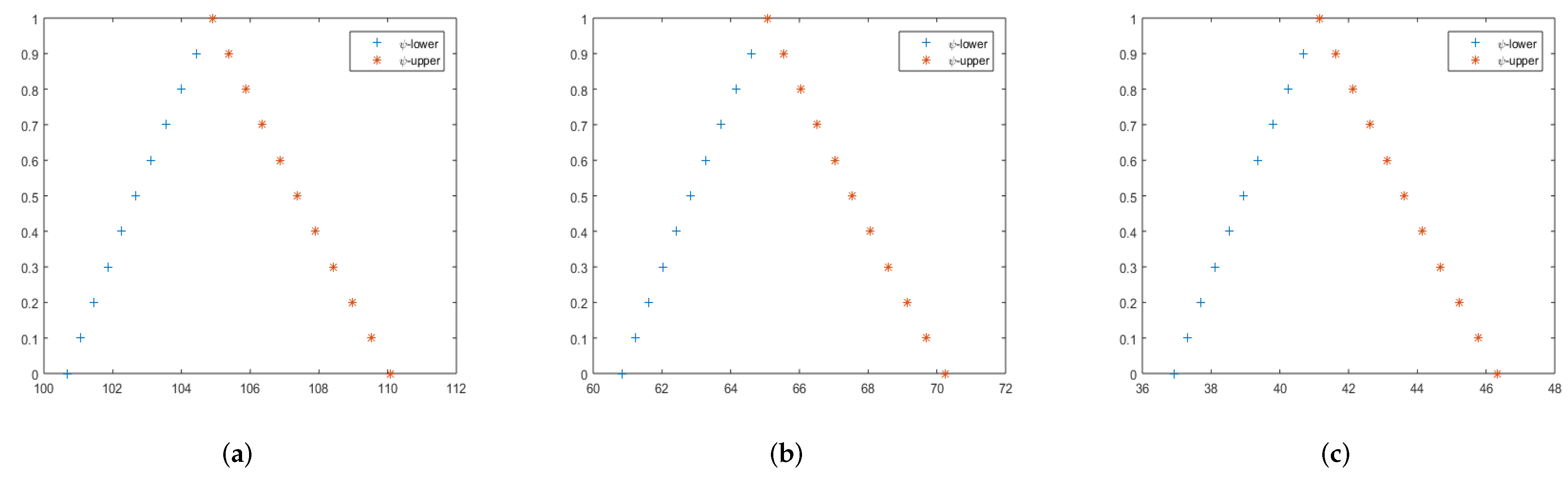
In Figure 3, we plot $2D$ graphs of the approximation solutions for fuzzy fractional diffusion equations (FFDEs) on the Cantor set. Figure 3a shows that for $\theta =1,\vartheta =3$, $n=1,\beta =0.25,0.50,0.75$, the FFDEs becomes bounded and closed. Moreover, the $\underline{\psi }$ sign shows increasing functions and $\overline{\psi }$ denotes decreasing functions on the $\varrho$-level set of $\psi$. To reflect the concept of the $\varrho$-level set, Figure 3a illustrates that the $\varrho$-level set of the FFDEs is bounded and closed for $\theta =1$. Similarly, in Figure 3b,c, we can observe the same explanation of the $\varrho$-level set closedness and boundedness for Example 4.

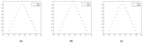
Figure 3. The approximate lower and upper solutions of (130) at (a–c) $\theta =1,\vartheta =3,n=1,\beta =0.25$, 0.50, 0.75, respectively. Moreover, (a–c) are 2D figures for the approximate solutions of the fuzzy fractional diffusion equation on the Cantor set of $\psi (\vartheta ,\theta )$ in Example 4.

Example 5.

We consider the following fuzzy fractional diffusion equation on the Cantor set

$$\begin{array}{c}\hfill \frac{{\partial }^{\beta }\psi (\vartheta ,\theta )}{\partial {\theta }^{\beta }}\ominus \frac{{\vartheta }^{2\beta }}{\mathsf{\Gamma }(1+2\beta )}\odot \frac{{\partial }^{2\beta }\psi (\vartheta ,\theta )}{\partial {\vartheta }^{2\beta }}=0,0<\beta \le 1,\end{array}$$

(143)

with the initial condition

$$\begin{array}{c}\hfill \psi (\vartheta ,0)=\left[{(0.75+0.25\varrho )}^n,{(1.25-0.25\varrho )}^n\right]\odot \left(\frac{{\vartheta }^{2\beta }}{\mathsf{\Gamma }(1+2\beta )}\right),\end{array}$$

(144)

where $n=1,2,3,\cdots .$

1. Local fuzzy fractional Laplace variational iteration method

Applying relation (103), the iterative relation is structured as follows:

$$\begin{array}{c}\hfill \begin{array}{cc}\hfill {Ł}_{\beta }\left\{{\psi }_{n+1}(\vartheta ,\theta )\right\}& ={Ł}_{\beta }\left\{{\psi }_n(\vartheta ,\theta )\right\}\ominus {Ł}_{\beta }\left\{1\right\}{Ł}_{\beta }\left\{\frac{{\partial }^{\beta }\psi (\vartheta ,\theta )}{\partial {\theta }^{\beta }}\ominus \frac{{\vartheta }^{2\beta }}{\mathsf{\Gamma }(1+2\beta )}\odot \frac{{\partial }^{2\beta }\psi (\vartheta ,\theta )}{\partial {\vartheta }^{2\beta }}\right\}\hfill \\ \hfill & ={Ł}_{\beta }\left\{{\psi }_n(\vartheta ,\theta )\right\}\ominus \frac{1}{s^{\beta }}\left(s^{\beta }{Ł}_{\beta }\left\{{\psi }_n(\vartheta ,\theta )\right\}\ominus {\psi }_n(\vartheta ,0)\ominus \frac{{\vartheta }^{2\beta }}{\mathsf{\Gamma }(1+2\beta )}\odot \frac{{\partial }^{2\beta }{Ł}_{\beta }\left\{\psi (\vartheta ,\theta )\right\}}{\partial {\vartheta }^{2\beta }}\right)\hfill \\ \hfill & =\frac{1}{s^{\beta }}{\psi }_n(\vartheta ,0)\oplus \frac{1}{s^{\beta }}\frac{{\vartheta }^{2\beta }}{\mathsf{\Gamma }(1+2\beta )}\odot \frac{{\partial }^{2\beta }{Ł}_{\beta }\left\{{\psi }_n(\vartheta ,\theta )\right\}}{\partial {\vartheta }^{2\beta }}.\hfill \end{array}\end{array}$$

(145)

According to (104), the initial value is

$$\begin{array}{c}\hfill \begin{array}{cc}\hfill {\psi }_0(\vartheta ,\theta )& =\left[{(0.75+0.25\varrho )}^n,{(1.25-0.25\varrho )}^n\right]\odot \left(\psi (\vartheta ,0)\oplus \frac{{\vartheta }^{\beta }}{\mathsf{\Gamma }(1+\beta )}\right),\hfill \\ \hfill {\psi }^{\left(\beta \right)}(\vartheta ,0)& =\left[{(0.75+0.25\varrho )}^n,{(1.25-0.25\varrho )}^n\right]\odot \left(\frac{{\vartheta }^{2\beta }}{\mathsf{\Gamma }(1+2\beta )}\right).\hfill \end{array}\end{array}$$

(146)

Thus, we obtain

$$\begin{array}{c}\hfill \begin{array}{cc}\hfill {Ł}_{\beta }\left\{{\psi }_1(\vartheta ,\theta )\right\}& =\frac{1}{s^{\beta }}{\psi }_0(\vartheta ,0)\oplus \frac{1}{s^{2\beta }}\frac{{\vartheta }^{2\beta }}{\mathsf{\Gamma }(1+2\beta )}\odot \frac{{\partial }^{2\beta }{Ł}_{\beta }\left\{{\psi }_0(\vartheta ,\theta )\right\}}{\partial {\vartheta }^{2\beta }},\hfill \\ \hfill & =\left[{(0.75+0.25\varrho )}^n,{(1.25-0.25\varrho )}^n\right]\odot \left(\frac{1}{s^{\beta }}\frac{{\vartheta }^{2\beta }}{\mathsf{\Gamma }(1+2\beta )}\oplus \frac{1}{s^{2\beta }}\frac{{\vartheta }^{2\beta }}{\mathsf{\Gamma }(1+2\beta )}\odot \frac{{\partial }^{2\beta }{Ł}_{\beta }}{\partial {\vartheta }^{2\beta }}\left\{\frac{{\vartheta }^{2\beta }}{\mathsf{\Gamma }(1+2\beta )}\right\}\right),\hfill \\ \hfill & =\left[{(0.75+0.25\varrho )}^n,{(1.25-0.25\varrho )}^n\right]\odot \frac{{\vartheta }^{2\beta }}{\mathsf{\Gamma }(1+2\beta )}\left(\frac{1}{s^{\beta }}\oplus \frac{1}{s^{3\beta }}\right).\hfill \end{array}\end{array}$$

(147)

Therefore,

$$\begin{array}{cc}\hfill {\psi }_1(\vartheta ,\theta )& =\left[{(0.75+0.25\varrho )}^n,{(1.25-0.25\varrho )}^n\right]\odot \left({Ł}_{\beta }^{-1}\left(\frac{{\vartheta }^{2\beta }}{\mathsf{\Gamma }(1+2\beta )}\left(\frac{1}{s^{\beta }}\oplus \frac{1}{s^{2\beta }}\right)\right)\right)\hfill \\ \hfill & =\left[{(0.75+0.25\varrho )}^n,{(1.25-0.25\varrho )}^n\right]\odot \frac{{\vartheta }^{2\beta }}{\mathsf{\Gamma }(1+2\beta )}\left(1\oplus \frac{{\theta }^{2\beta }}{\mathsf{\Gamma }(1+2\beta )}\right).\hfill \end{array}$$

(148)

The second approximation is written as

$$\begin{array}{c}\hfill \begin{array}{cc}\hfill {Ł}_{\beta }\left\{{\psi }_2(\vartheta ,\theta )\right\}& =\frac{1}{s^{\beta }}{\psi }_1(\vartheta ,0)\oplus \frac{1}{s^{\beta }}\frac{{\vartheta }^{2\beta }}{\mathsf{\Gamma }(1+2\beta )}\odot \frac{{\partial }^{2\beta }{Ł}_{\beta }\left\{{\psi }_1(\vartheta ,\theta )\right\}}{\partial {\vartheta }^{2\beta }},\hfill \\ \hfill & =\left[{(0.75+0.25\varrho )}^n,{(1.25-0.25\varrho )}^n\right]\odot \left(\frac{1}{s^{\beta }}\frac{{\vartheta }^{2\beta }}{\mathsf{\Gamma }(1+2\beta )}\oplus \frac{1}{s^{\beta }}\frac{{\vartheta }^{2\beta }}{\mathsf{\Gamma }(1+2\beta )}\right.\hfill \\ \hfill & \left.\odot \frac{{\partial }^{2\beta }{Ł}_{\beta }}{\partial {\vartheta }^{2\beta }}\left\{\frac{{\vartheta }^{2\beta }}{\mathsf{\Gamma }(1+2\beta )}\left(1\oplus \frac{{\theta }^{\beta }}{\mathsf{\Gamma }(1+\beta )}\right)\right\}\right),\hfill \\ \hfill & =\left[{(0.75+0.25\varrho )}^n,{(1.25-0.25\varrho )}^n\right]\odot \frac{{\vartheta }^{2\beta }}{\mathsf{\Gamma }(1+2\beta )}\left(\frac{1}{s^{\beta }}\oplus \frac{1}{s^{2\beta }}\oplus \frac{1}{s^{3\beta }}\right).\hfill \end{array}\end{array}$$

Thus, we have

$$\begin{array}{cc}\hfill {\psi }_1(\vartheta ,\theta )& =\left[{(0.75+0.25\varrho )}^n,{(1.25-0.25\varrho )}^n\right]\odot \left({Ł}_{\beta }^{-1}\left(\frac{{\vartheta }^{2\beta }}{\mathsf{\Gamma }(1+2\beta )}\left(\frac{1}{s^{\beta }}\oplus \frac{1}{s^{2\beta }}\oplus \frac{1}{s^{3\beta }}\right)\right)\right)\hfill \\ \hfill & =\left[{(0.75+0.25\varrho )}^n,{(1.25-0.25\varrho )}^n\right]\odot \frac{{\vartheta }^{2\beta }}{\mathsf{\Gamma }(1+2\beta )}\left(1\oplus \frac{{\theta }^{\beta }}{\mathsf{\Gamma }(1+\beta )}\oplus \frac{t^{2\beta }}{\mathsf{\Gamma }(1+2\beta )}\right),\hfill \end{array}$$

(149)

which gives us the local fuzzy fractional series solutions

$$\begin{array}{c}\hfill \begin{array}{cc}\hfill \psi (\vartheta ,\theta )& =\underset{n\to \infty }{\lim }{Ł}_{\beta }^{-1}\left({}_{\beta }\left\{{\psi }_n(\vartheta ,\theta )\right\}\right),\hfill \\ \hfill & =\left[{(0.75+0.25\varrho )}^n,{(1.25-0.25\varrho )}^n\right]\odot \left(\underset{n\to \infty }{\lim }{Ł}_{\beta }^{-1}\left(\frac{{\vartheta }^{2\beta }}{\mathsf{\Gamma }(1+2\beta )}\sum _{k=0}^n\frac{1}{s^{(n+1)\beta }}\right)\right)\hfill \\ \hfill & =\left[{(0.75+0.25\varrho )}^n,{(1.25-0.25\varrho )}^n\right]\odot \left(\underset{n\to \infty }{\lim }\frac{{\vartheta }^{2\beta }}{\mathsf{\Gamma }(1+2\beta )}\sum _{k=0}^n\frac{{\theta }^{k\beta }}{\mathsf{\Gamma }(1+2\beta )}\right)\hfill \\ \hfill & =\left[{(0.75+0.25\varrho )}^n,{(1.25-0.25\varrho )}^n\right]\odot \left(\frac{{\vartheta }^{2\beta }}{\mathsf{\Gamma }(1+2\beta )}\sum _{k=0}^{\infty }\frac{{\theta }^{k\beta }}{\mathsf{\Gamma }(1+2\beta )}\right).\hfill \end{array}\end{array}$$

(150)

Hence, we find our desired solution as

$$\begin{array}{c}\hfill \psi (\vartheta ,\theta )=\left[{(0.75+0.25\varrho )}^n,{(1.25-0.25\varrho )}^n\right]\odot \left(\frac{{\vartheta }^{2\beta }}{\mathsf{\Gamma }(1+2\beta )}{E}_{\beta }\left({\theta }^{\beta }\right)\right).\end{array}$$

(151)

2. Local fuzzy fractional series expansion method

Following (114), we have

$$\begin{array}{c}\hfill \begin{array}{cc}\hfill X_{i+1}\left(\vartheta \right)& =\left[{(0.75+0.25\varrho )}^n,{(1.25-0.25\varrho )}^n\right]\odot \left(\frac{{\vartheta }^{2\beta }}{\mathsf{\Gamma }(1+2\beta )}\frac{{\partial }^{2\beta }{X}_i\left(\vartheta \right)}{\partial {\vartheta }^{2\beta }}\right),\hfill \\ \hfill X_0\left(\vartheta \right)& =\left[{(0.75+0.25\varrho )}^n,{(1.25-0.25\varrho )}^n\right]\odot \left(\frac{{\vartheta }^{2\beta }}{\mathsf{\Gamma }(1+2\beta )}\right),\hfill \end{array}\end{array}$$

(152)

We apply the recursive formula (152) to get

$$\begin{array}{c}\hfill \begin{array}{cc}\hfill X_0\left(\vartheta \right)& =\left[{(0.75+0.25\varrho )}^n,{(1.25-0.25\varrho )}^n\right]\odot \left(\frac{{\vartheta }^{2\beta }}{\mathsf{\Gamma }(1+2\beta )}\right),\hfill \\ \hfill X_1\left(\vartheta \right)& =\left[{(0.75+0.25\varrho )}^n,{(1.25-0.25\varrho )}^n\right]\odot \left(\frac{{\vartheta }^{2\beta }}{\mathsf{\Gamma }(1+2\beta )}\right),\hfill \\ \hfill X_2\left(\vartheta \right)& =\left[{(0.75+0.25\varrho )}^n,{(1.25-0.25\varrho )}^n\right]\odot \left(\frac{{\vartheta }^{2\beta }}{\mathsf{\Gamma }(1+2\beta )}\right),\hfill \\ \hfill & ⋮.\hfill \end{array}\end{array}$$

(153)

As a result of these recursive calculations, one can obtain

$$\begin{array}{c}\hfill \begin{array}{cc}\hfill \psi (\vartheta ,\theta )& =\left[{(0.75+0.25\varrho )}^n,{(1.25-0.25\varrho )}^n\right]\odot \left(\frac{{\vartheta }^{2\beta }}{\mathsf{\Gamma }(1+2\beta )}\sum _{k=0}^{\infty }\frac{{\theta }^{k\beta }}{\mathsf{\Gamma }(1+2\beta )}\right),\hfill \\ \hfill \psi (\vartheta ,\theta )& =\left[{(0.75+0.25\varrho )}^n,{(1.25-0.25\varrho )}^n\right]\odot \left(\frac{{\vartheta }^{2\beta }}{\mathsf{\Gamma }(1+2\beta )}{E}_{\beta }\left({\theta }^{\beta }\right)\right).\hfill \end{array}\end{array}$$

(154)

Table 5 shows the error term between exact and approximate solutions of Example 5. for $\beta =0.50,1.$

Table 5. For the absolute error between exact solutions (E-S) at $\beta =1$ and approximate solutions (A-S) at $\beta =0.50$.

$\mathit{\varrho }$	Lower E-S	Lower A-S	Lower Error	Upper E-S	Upper A-S	Upper Error
0	838.39	161.01	677.39	2328.9	447.25	1881.6
0.1	895.22	171.92	723.3	2236.7	429.54	1807.1
0.2	953.91	183.19	770.71	2146.3	412.18	1734.1
0.3	1014.5	194.82	819.64	2057.8	395.19	1662.6
0.4	1076.9	206.81	870.06	1971.2	378.55	1592.6
0.5	1141.1	219.15	922	1886.4	362.27	1524.1
0.6	1207.3	231.85	975.44	1803.5	346.35	1457.1
0.7	1275.3	244.91	1030.4	1722.4	330.78	1391.7
0.8	1345.2	258.33	1086.8	1643.3	315.58	1327.7
0.9	1416.9	272.1	1144.8	1565.9	300.73	1265.2
1	1490.5	286.24	1204.2	1490.5	286.24	1204.2

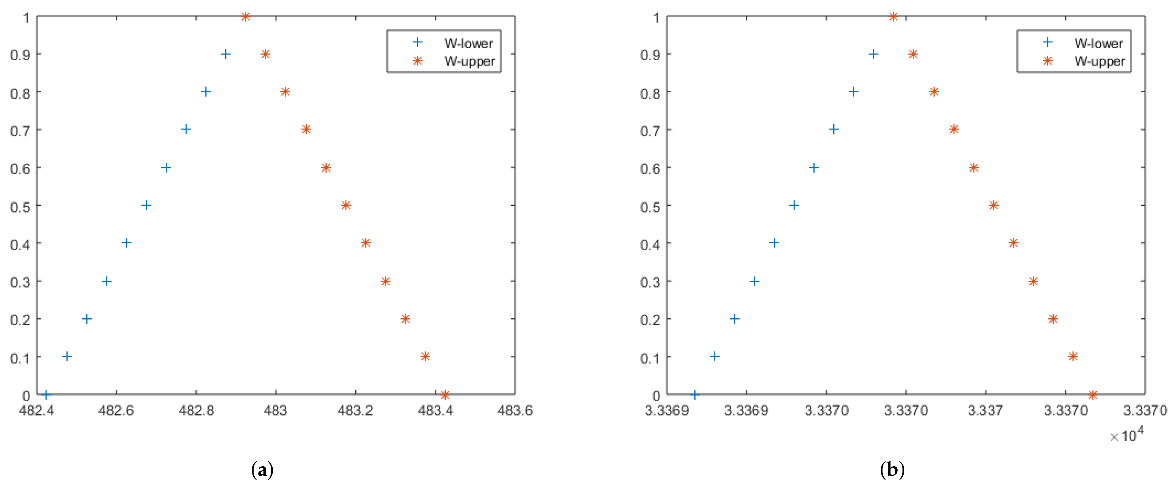
In Figure 4, we plot $2D$ graphs of the exact and approximation solutions of local fuzzy fractional diffusion equation on Cantor set. Figure 4a shows that for $\theta =8,\vartheta =1,\beta =1$, $n=2$, the local fuzzy fractional diffusion equation on Cantor set become bounded and closed. In addition, the $\underline{\psi }$ sign shows increasing functions and $\overline{\psi }$ denotes decreasing functions on the $\varrho$-level set of $\psi$. To reflect the concept of the $\varrho$-level set, Figure 4a illustrates that the $\varrho$-level set of local fuzzy fractional diffusion equation on Cantor set is bounded and closed for $\theta =8$. Similarly, in Figure 4b, we can observe the same explanation of $\varrho$-level set closedness and boundedness for Example 5.

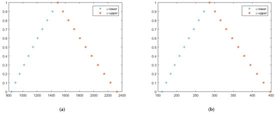
Figure 4. The exact and approximate lower and upper solutions of (143) at (a) $\theta =8,\vartheta =1,\beta =1,n=2$ (b) $\theta =8,\vartheta =1,\beta =0.50,n=2$. Further, (a,b) 2D figures for the exact and approximate solutions of fuzzy fractional diffusion equation on Cantor set of $\psi (\vartheta ,\theta )$ in Example 5.

Example 6.

We consider the following fuzzy fractional wave equation on a Cantor set

$$\begin{array}{c}\hfill \frac{{\partial }^{2\beta }\psi (\vartheta ,\theta )}{\partial {\theta }^{2\beta }}\ominus \frac{{\vartheta }^{2\beta }}{\mathsf{\Gamma }(1+2\beta )}\odot \frac{{\partial }^{2\beta }\psi (\vartheta ,\theta )}{\partial {\vartheta }^{2\beta }}=0,1<\beta \le 2,\end{array}$$

(155)

subject to the initial value condition

$$\begin{array}{c}\hfill \begin{array}{cc}\hfill & \psi (\vartheta ,0)=\left[{(2.25+0.25\varrho )}^n,{(2.75-0.25\varrho )}^n\right]\oplus \left(\frac{{\vartheta }^{2\beta }}{\mathsf{\Gamma }(1+2\beta )}\right),\hfill \\ \hfill & \frac{{\partial }^{\beta }\psi (\vartheta ,0)}{\partial {\theta }^{\beta }}=\left[{(2.25+0.25\varrho )}^n,{(2.75-0.25\varrho )}^n\right],\hfill \end{array}\end{array}$$

(156)

where $n=1,2,3,\cdots .$

1. Local fuzzy fractional Laplace variational iteration method

Using relation (103), we structure the iterative relation as

$$\begin{array}{c}\hfill \begin{array}{cc}\hfill {Ł}_{\beta }\left\{{\psi }_{n+1}(\vartheta ,\theta )\right\}& ={Ł}_{\beta }\left\{{\psi }_n(\vartheta ,\theta )\right\}\ominus {Ł}_{\beta }\left\{\frac{{\theta }^{\beta }}{\mathsf{\Gamma }(1+\beta )}\right\}{Ł}_{\beta }\left\{\frac{{\partial }^{2\beta }\psi (\vartheta ,\theta )}{\partial {\theta }^{2\beta }}\ominus \frac{{\vartheta }^{2\beta }}{\mathsf{\Gamma }(1+2\beta )}\odot \frac{{\partial }^{2\beta }\psi (\vartheta ,\theta )}{\partial {\vartheta }^{2\beta }}\right\}\hfill \\ \hfill & ={Ł}_{\beta }\left\{{\psi }_n(\vartheta ,\theta )\right\}\ominus \frac{1}{s^{2\beta }}\left(s^{2\beta }{Ł}_{\beta }\left\{{\psi }_n(\vartheta ,\theta )\right\}\right.\hfill \\ \hfill & \left.\ominus s^{\beta }{\psi }_n(\vartheta ,0)\ominus {\psi }_n^{\left(\beta \right)}(\vartheta ,0)\ominus \frac{{\vartheta }^{2\beta }}{\mathsf{\Gamma }(1+2\beta )}\odot \frac{{\partial }^{2\beta }{Ł}_{\beta }\left\{{\psi }_n(\vartheta ,\theta )\right\}}{\partial {\vartheta }^{2\beta }}\right)\hfill \\ \hfill & =\frac{1}{s^{\beta }}{\psi }_n(\vartheta ,0)\oplus \frac{1}{s^{2\beta }}{\psi }_n^{\left(\beta \right)}(\vartheta ,0)\oplus \frac{1}{s^{2\beta }}\frac{{\vartheta }^{2\beta }}{\mathsf{\Gamma }(1+2\beta )}\odot \frac{{\partial }^{2\beta }{Ł}_{\beta }\left\{{\psi }_n(\vartheta ,\theta )\right\}}{\partial {\vartheta }^{2\beta }}.\hfill \end{array}\end{array}$$

According to (104), the initial value is

$$\begin{array}{c}\hfill {\psi }_0(\vartheta ,\theta )=\psi (\vartheta ,\theta )\oplus {\psi }^{\left(\beta \right)}(\vartheta ,0)=\left[{(2.25+0.25\varrho )}^n,{(2.75-0.25\varrho )}^n\right]\oplus \left(\frac{{\vartheta }^{2\beta }}{\mathsf{\Gamma }(1+2\beta )}\right).\end{array}$$

(157)

Hence, we obtain the first approximation

$$\begin{array}{c}\hfill \begin{array}{cc}\hfill {Ł}_{\beta }\left\{{\psi }_1(\vartheta ,\theta )\right\}& =\frac{1}{s^{\beta }}{\psi }_0(\vartheta ,0)\oplus \frac{1}{s^{2\beta }}{\psi }_0^{\left(\beta \right)}(\vartheta ,0)\oplus \frac{1}{s^{2\beta }}\frac{{\vartheta }^{2\beta }}{\mathsf{\Gamma }(1+2\beta )}\odot \frac{{\partial }^{2\beta }{Ł}_{\beta }\left\{{\psi }_0(\vartheta ,\theta )\right\}}{\partial {\vartheta }^{2\beta }},\hfill \\ \hfill & =\left[{(2.25+0.25\varrho )}^n,{(2.75-0.25\varrho )}^n\right]\oplus \left(\frac{1}{s^{\beta }}\frac{{\vartheta }^{2\beta }}{\mathsf{\Gamma }(1+2\beta )}\oplus \frac{1}{s^{\beta }}\frac{{\vartheta }^{2\beta }}{\mathsf{\Gamma }(1+2\beta )}\odot \frac{{\partial }^{2\beta }{Ł}_{\beta }}{\partial {\vartheta }^{2\beta }}\left\{\frac{{\vartheta }^{2\beta }}{\mathsf{\Gamma }(1+2\beta )}\right\}\right),\hfill \\ \hfill & =\left[{(2.25+0.25\varrho )}^n,{(2.75-0.25\varrho )}^n\right]\oplus \frac{{\vartheta }^{2\beta }}{\mathsf{\Gamma }(1+2\beta )}\left(\frac{1}{s^{\beta }}\oplus \frac{1}{s^{3\beta }}\right).\hfill \end{array}\end{array}$$

(158)

Thus,

$$\begin{array}{cc}\hfill {\psi }_1(\vartheta ,\theta )& =\left[{(2.25+0.25\varrho )}^n,{(2.75-0.25\varrho )}^n\right]\oplus \left({Ł}_{\beta }^{-1}\left(\frac{{\vartheta }^{2\beta }}{\mathsf{\Gamma }(1+2\beta )}\left(\frac{1}{s^{\beta }}\oplus \frac{1}{s^{3\beta }}\right)\right)\right)\hfill \\ \hfill & =\left[{(2.25+0.25\varrho )}^n,{(2.75-0.25\varrho )}^n\right]\oplus \frac{{\vartheta }^{2\beta }}{\mathsf{\Gamma }(1+2\beta )}\left(1\oplus \frac{{\theta }^{2\beta }}{\mathsf{\Gamma }(1+2\beta )}\right).\hfill \end{array}$$

(159)

The second approximation can be written as

$$\begin{array}{c}\hfill \begin{array}{cc}\hfill {Ł}_{\beta }\left\{{\psi }_2(\vartheta ,\theta )\right\}& =\frac{1}{s^{\beta }}{\psi }_1(\vartheta ,0)\oplus \frac{1}{s^{2\beta }}{\psi }_1^{\left(\beta \right)}(\vartheta ,0)\oplus \frac{1}{s^{2\beta }}\frac{{\vartheta }^{2\beta }}{\mathsf{\Gamma }(1+2\beta )}\odot \frac{{\partial }^{2\beta }{Ł}_{\beta }\left\{{\psi }_1(\vartheta ,\theta )\right\}}{\partial {\vartheta }^{2\beta }},\hfill \\ \hfill & =\left[{(2.25+0.25\varrho )}^n,{(2.75-0.25\varrho )}^n\right]\oplus \left(\frac{1}{s^{\beta }}\frac{{\vartheta }^{2\beta }}{\mathsf{\Gamma }(1+2\beta )}\oplus \frac{1}{s^{2\beta }}\frac{{\vartheta }^{2\beta }}{\mathsf{\Gamma }(1+2\beta )}\right.\hfill \\ \hfill & \left.\odot \frac{{\partial }^{2\beta }}{\partial {\vartheta }^{2\beta }}{Ł}_{\beta }\left\{\frac{{\vartheta }^{2\beta }}{\mathsf{\Gamma }(1+2\beta )}\left(1\oplus \frac{{\theta }^{2\beta }}{\mathsf{\Gamma }(1+2\beta )}\right)\right\}\right),\hfill \\ \hfill & =\left[{(2.25+0.25\varrho )}^n,{(2.75-0.25\varrho )}^n\right]\oplus \frac{{\vartheta }^{2\beta }}{\mathsf{\Gamma }(1\oplus 2\beta )}\left(\frac{1}{s^{\beta }}\oplus \frac{1}{s^{3\beta }}\oplus \frac{1}{s^{5\beta }}\right).\hfill \end{array}\end{array}$$

We obtain

$$\begin{array}{cc}\hfill {\psi }_2(\vartheta ,\theta )& =\left[{(2.25+0.25\varrho )}^n,{(2.75-0.25\varrho )}^n\right]\oplus \left({Ł}_{\beta }^{-1}\left(\frac{{\vartheta }^{2\beta }}{\mathsf{\Gamma }(1+2\beta )}\left(\frac{1}{s^{\beta }}\oplus \frac{1}{s^{3\beta }}\oplus \frac{1}{s^{5\beta }}\right)\right)\right)\hfill \\ \hfill & =\left[{(2.25+0.25\varrho )}^n,{(2.75-0.25\varrho )}^n\right]\oplus \frac{{\vartheta }^{2\beta }}{\mathsf{\Gamma }(1+2\beta )}\left(1\oplus \frac{{\theta }^{2\beta }}{\mathsf{\Gamma }(1+2\beta )}\oplus \frac{{\theta }^{4\beta }}{\mathsf{\Gamma }(1+4\beta )}\right).\hfill \end{array}$$

(160)

The local fuzzy fractional series solutions are

$$\begin{array}{c}\hfill \begin{array}{cc}\hfill \psi (\vartheta ,\theta )& =\underset{n\to \infty }{\lim }{Ł}_{\beta }^{-1}\left({}_{\beta }\left\{{\psi }_n(\vartheta ,\theta )\right\}\right),\hfill \\ \hfill & =\left[{(2.25+0.25\varrho )}^n,{(2.75-0.25\varrho )}^n\right]\oplus \left(\underset{n\to \infty }{\lim }{Ł}_{\beta }^{-1}\left(\frac{{\vartheta }^{2\beta }}{\mathsf{\Gamma }(1+2\beta )}\sum _{k=0}^n\frac{1}{s^{(2n+1)\beta }}\right)\right)\hfill \\ \hfill & =\left[{(2.25+0.25\varrho )}^n,{(2.75-0.25\varrho )}^n\right]\oplus \left(\underset{n\to \infty }{\lim }\frac{{\vartheta }^{2\beta }}{\mathsf{\Gamma }(1+2\beta )}\sum _{k=0}^n\frac{{\theta }^{2k\beta }}{\mathsf{\Gamma }(1+2k\beta )}\right)\hfill \\ \hfill & =\left[{(2.25+0.25\varrho )}^n,{(2.75-0.25\varrho )}^n\right]\oplus \left(\frac{{\vartheta }^{2\beta }}{\mathsf{\Gamma }(1+2\beta )}\sum _{k=0}^{\infty }\frac{{\theta }^{k\beta }}{\mathsf{\Gamma }(1+k\beta )}\right).\hfill \end{array}\end{array}$$

(161)

Thus, we can obtain the solutions as

$$\begin{array}{c}\hfill \psi (\vartheta ,\theta )=\left[{(2.25+0.25\varrho )}^n,{(2.75-0.25\varrho )}^n\right]\oplus \left(\frac{{\vartheta }^{2\beta }}{\mathsf{\Gamma }(1+2\beta )}{\cosh }_{\beta }\left({\theta }^{\beta }\right)\right).\end{array}$$

(162)

2. Local fuzzy fractional variation iteration method

Using (121), we have the iterative formula

$$\begin{array}{cc}\hfill {\psi }_{n+1}(\vartheta ,\theta )& ={\psi }_n(\vartheta ,\theta )\oplus \frac{1}{\mathsf{\Gamma }(1+\beta )}{\int }_0^{\theta }\frac{{(s-\theta )}^{\beta }}{\mathsf{\Gamma }(1+\beta )}\odot \frac{{\partial }^{2\beta }{\psi }_n(\vartheta ,\theta )}{\partial s^{2\beta }}{\left(ds\right)}^{\beta }\hfill \\ \hfill & \ominus \frac{1}{\mathsf{\Gamma }(1+\beta )}\odot {\int }_0^{\theta }\frac{{(s-\theta )}^{\beta }}{\mathsf{\Gamma }(1+\beta )}\odot \frac{{\vartheta }^{2\beta }}{\mathsf{\Gamma }(1+2\beta )}\odot \frac{{\partial }^{2\beta }{\psi }_n(\vartheta ,\theta )}{\partial {\vartheta }^{2\beta }}{\left(ds\right)}^{\beta },\hfill \end{array}$$

(163)

where the initial condition is defined as

$$\begin{array}{cc}\hfill {\psi }_0(\vartheta ,\theta )& =\left[{(2.25+0.25\varrho )}^n,{(2.75-0.25\varrho )}^n\right]\oplus \left(\frac{{\vartheta }^{2\beta }}{\mathsf{\Gamma }(1+2\beta )}\right).\hfill \end{array}$$

(164)

After computing (156), we have

$$\begin{array}{c}\hfill \begin{array}{cc}\hfill {\psi }_1(\vartheta ,\theta )& ={\psi }_0(\vartheta ,\theta )\oplus \frac{1}{\mathsf{\Gamma }(1+\beta )}\odot {\int }_0^{\theta }\frac{{(s-\theta )}^{\beta }}{\mathsf{\Gamma }(1+\beta )}\odot \frac{{\partial }^{2\beta }{\psi }_0(\vartheta ,\theta )}{\partial s^{2\beta }}{\left(ds\right)}^{\beta }\hfill \\ \hfill & \ominus \frac{1}{\mathsf{\Gamma }(1+\beta )}\odot {\int }_0^{\theta }\frac{{(s-\theta )}^{\beta }}{\mathsf{\Gamma }(1+\beta )}\odot \frac{{\vartheta }^{2\beta }}{\mathsf{\Gamma }(1+2\beta )}\odot \frac{{\partial }^{2\beta }{\psi }_0(\vartheta ,\theta )}{\partial {\vartheta }^{2\beta }}{\left(ds\right)}^{\beta }\hfill \\ \hfill & ={\psi }_0(\vartheta ,\theta )\oplus \frac{1}{\mathsf{\Gamma }(1+\beta )}\odot {\int }_0^{\theta }\frac{{(s-\theta )}^{\beta }}{\mathsf{\Gamma }(1+\beta )}\odot \left[-\left(\left[{(2.25+0.25\varrho )}^n,{(2.75-0.25\varrho )}^n\right]\oplus \left(\frac{{\vartheta }^{2\beta }}{\mathsf{\Gamma }(1+2\beta )}\right)\right)\right]{\left(ds\right)}^{\beta }\hfill \\ \hfill & =\left[{(2.25+0.25\varrho )}^n,{(2.75-0.25\varrho )}^n\right]\oplus \left[\frac{{\vartheta }^{2\beta }}{\mathsf{\Gamma }(1+2\beta )}\left(1\oplus \frac{{\theta }^{2\beta }}{\mathsf{\Gamma }(1+2\beta )}\right)\right],\hfill \end{array}\end{array}$$

$$\begin{array}{c}\hfill \begin{array}{cc}\hfill {\psi }_2(\vartheta ,\theta )& ={\psi }_1(\vartheta ,\theta )\oplus \frac{1}{\mathsf{\Gamma }(1+\beta )}\odot {\int }_0^{\theta }\frac{{(s-\theta )}^{\beta }}{\mathsf{\Gamma }(1+\beta )}\odot \frac{{\partial }^{2\beta }{\psi }_1(\vartheta ,\theta )}{\partial s^{2\beta }}{\left(ds\right)}^{\beta }\hfill \\ \hfill & \ominus \frac{1}{\mathsf{\Gamma }(1+\beta )}\odot {\int }_0^{\theta }\frac{{(s-\theta )}^{\beta }}{\mathsf{\Gamma }(1+\beta )}\odot \frac{{\vartheta }^{2\beta }}{\mathsf{\Gamma }(1+2\beta )}\odot \frac{{\partial }^{2\beta }{\psi }_1(\vartheta ,\theta )}{\partial {\vartheta }^{2\beta }}{\left(ds\right)}^{\beta }\hfill \\ \hfill & ={\psi }_1(\vartheta ,\theta )\oplus \frac{1}{\mathsf{\Gamma }(1+\beta )}\odot {\int }_0^{\theta }\frac{{(s-\theta )}^{\beta }}{\mathsf{\Gamma }(1+\beta )}\hfill \\ \hfill & \odot \left[-\left(\left[{(2.25+0.25\varrho )}^n,{(2.75-0.25\varrho )}^n\right]\oplus \left(\frac{{\vartheta }^{2\beta }}{\mathsf{\Gamma }(1+2\beta )}\frac{s^{2\beta }}{\mathsf{\Gamma }(1+2\beta )}\right)\right)\right]{\left(ds\right)}^{\beta }\hfill \\ \hfill & =\left[{(2.25+0.25\varrho )}^n,{(2.75-0.25\varrho )}^n\right]\oplus \left[\frac{{\vartheta }^{2\beta }}{\mathsf{\Gamma }(1+2\beta )}\left(1\oplus \frac{{\theta }^{2\beta }}{\mathsf{\Gamma }(1+2\beta )}\oplus \frac{{\theta }^{4\beta }}{\mathsf{\Gamma }(1+4\beta )}\right)\right],\hfill \end{array}\end{array}$$

$$\begin{array}{c}\hfill \begin{array}{cc}\hfill {\psi }_3(\vartheta ,\theta )& ={\psi }_2(\vartheta ,\theta )\oplus \frac{1}{\mathsf{\Gamma }(1+\beta )}\odot {\int }_0^{\theta }\frac{{(s-\theta )}^{\beta }}{\mathsf{\Gamma }(1+\beta )}\odot \frac{{\partial }^{2\beta }{\psi }_2(\vartheta ,\theta )}{\partial s^{2\beta }}{\left(ds\right)}^{\beta }\hfill \\ \hfill & \ominus \frac{1}{\mathsf{\Gamma }(1+\beta )}\odot {\int }_0^{\theta }\frac{{(s-\theta )}^{\beta }}{\mathsf{\Gamma }(1+\beta )}\odot \frac{{\vartheta }^{2\beta }}{\mathsf{\Gamma }(1+2\beta )}\odot \frac{{\partial }^{2\beta }{\psi }_2(\vartheta ,\theta )}{\partial {\vartheta }^{2\beta }}{\left(ds\right)}^{\beta }\hfill \\ \hfill & ={\psi }_2(\vartheta ,\theta )\oplus \frac{1}{\mathsf{\Gamma }(1+\beta )}\odot {\int }_0^{\theta }\frac{{(s-\theta )}^{\beta }}{\mathsf{\Gamma }(1+\beta )}\hfill \\ \hfill & \odot \left[-\left(\left[{(2.25+0.25\varrho )}^n,{(2.75-0.25\varrho )}^n\right]\oplus \left(\frac{{\vartheta }^{2\beta }}{\mathsf{\Gamma }(1+2\beta )}\frac{{\theta }^{4\beta }}{\mathsf{\Gamma }(1+4\beta )}\right)\right)\right]{\left(ds\right)}^{\beta }\hfill \\ \hfill & =\left[{(2.25+0.25\varrho )}^n,{(2.75-0.25\varrho )}^n\right]\oplus \left[\frac{{\vartheta }^{2\beta }}{\mathsf{\Gamma }(1+2\beta )}\sum _{i=0}^3\frac{{\theta }^{2i\beta }}{\mathsf{\Gamma }(1+2i\beta )}\right],\hfill \\ \hfill & ⋮\hfill \end{array}\end{array}$$

$$\begin{array}{c}\hfill \begin{array}{cc}\hfill {\psi }_n(\vartheta ,\theta )& ={\psi }_{n-1}(\vartheta ,\theta )\oplus \frac{1}{\mathsf{\Gamma }(1+\beta )}\odot {\int }_0^{\theta }\frac{{(s-\theta )}^{\beta }}{\mathsf{\Gamma }(1+\beta )}\odot \frac{{\partial }^{2\beta }{\psi }_{n-1}(\vartheta ,\theta )}{\partial s^{2\beta }}{\left(ds\right)}^{\beta }\hfill \\ \hfill & \ominus \frac{1}{\mathsf{\Gamma }(1+\beta )}\odot {\int }_0^{\theta }\frac{{(s-\theta )}^{\beta }}{\mathsf{\Gamma }(1+\beta )}\odot \frac{{\vartheta }^{2\beta }}{\mathsf{\Gamma }(1+2\beta )}\odot \frac{{\partial }^{2\beta }{\psi }_{n-1}(\vartheta ,\theta )}{\partial {\vartheta }^{2\beta }}{\left(ds\right)}^{\beta }\hfill \\ \hfill & =\left[{(2.25+0.25\varrho )}^n,{(2.75-0.25\varrho )}^n\right]\oplus \left[\frac{{\vartheta }^{2\beta }}{\mathsf{\Gamma }(1+2\beta )}\sum _{i=0}^n\frac{{\theta }^{2i\beta }}{\mathsf{\Gamma }(1+2i\beta )}\right].\hfill \end{array}\end{array}$$

(165)

Consequently, we obtain the solution as follows:

$$\begin{array}{c}\hfill \psi (\vartheta ,\theta )=\underset{n\to }{\lim }{\psi }_n\left(\vartheta \right)=\left[{(2.25+0.25\varrho )}^n,{(2.75-0.25\varrho )}^n\right]\oplus \left[\frac{{\vartheta }^{2\beta }}{\mathsf{\Gamma }(1+2\beta )}{\cosh }_{\beta }\left({\theta }^{\beta }\right)\right].\end{array}$$

(166)

3. Local fuzzy fractional decomposition method

From (128), we obtain

$$\begin{array}{c}\hfill \begin{array}{cc}\hfill {\psi }_{n+1}(\vartheta ,\theta )& ={}_0{\mathbb{I}}_{\theta }^{\left(\beta \right)}{}_0{\mathbb{I}}_{\theta }^{\left(\beta \right)}\frac{{\vartheta }^{2\beta }}{\mathsf{\Gamma }(1+2\beta )}\frac{{\partial }^{2\beta }{\psi }_n(\vartheta ,\theta )}{\partial {\vartheta }^{2\beta }},\hfill \\ \hfill {\psi }_0(\vartheta ,\theta )& =\left[{(2.25+0.25\varrho )}^n,{(2.75-0.25\varrho )}^n\right]\oplus \frac{{\vartheta }^{2\beta }}{\mathsf{\Gamma }(1+2\beta )}.\hfill \end{array}\end{array}$$

(167)

From (167), the components are

$$\begin{array}{c}\hfill \begin{array}{cc}\hfill {\psi }_0(\vartheta ,\theta )& =\left[{(2.25+0.25\varrho )}^n,{(2.75-0.25\varrho )}^n\right]\oplus \left[\frac{{\vartheta }^{2\beta }}{\mathsf{\Gamma }(1+2\beta )}\right],\hfill \\ \hfill {\psi }_1(\vartheta ,\theta )& =\left[{(2.25+0.25\varrho )}^n,{(2.75-0.25\varrho )}^n\right]\oplus \left[\frac{{\vartheta }^{2\beta }}{\mathsf{\Gamma }(1+2\beta )}\odot \frac{{\theta }^{2\beta }}{\mathsf{\Gamma }(1+2\beta )}\right],\hfill \\ \hfill {\psi }_2(\vartheta ,\theta )& =\left[{(2.25+0.25\varrho )}^n,{(2.75-0.25\varrho )}^n\right]\oplus \left[\frac{{\vartheta }^{2\beta }}{\mathsf{\Gamma }(1+2\beta )}\odot \frac{{\theta }^{4\beta }}{\mathsf{\Gamma }(1+4\beta )}\right],\hfill \\ \hfill {\psi }_3(\vartheta ,\theta )& =\left[{(2.25+0.25\varrho )}^n,{(2.75-0.25\varrho )}^n\right]\oplus \left[\frac{{\vartheta }^{2\beta }}{\mathsf{\Gamma }(1+2\beta )}\odot \frac{{\theta }^{3\beta }}{\mathsf{\Gamma }(1+3\beta )}\right],\hfill \\ \hfill {\psi }_4(\vartheta ,\theta )& =\left[{(2.25+0.25\varrho )}^n,{(2.75-0.25\varrho )}^n\right]\oplus \left[\frac{{\vartheta }^{2\beta }}{\mathsf{\Gamma }(1+2\beta )}\odot \frac{{\theta }^{8\beta }}{\mathsf{\Gamma }(1+8\beta )}\right],\hfill \\ \hfill & ⋮\hfill \\ \hfill {\psi }_{\kappa }(\vartheta ,\theta )& =\left[{(2.25+0.25\varrho )}^n,{(2.75-0.25\varrho )}^n\right]\oplus \left[\frac{{\vartheta }^{2\beta }}{\mathsf{\Gamma }(1+2\beta )}\odot \frac{{\theta }^{2\kappa \beta }}{\mathsf{\Gamma }(1+2\kappa \beta )}\right].\hfill \end{array}\end{array}$$

(168)

Thus, the exact solution can be defined as

$$\begin{array}{c}\hfill \begin{array}{cc}\hfill \psi (\vartheta ,\theta )& =\underset{n\to \infty }{\lim }\sum _{\kappa =0}^{\infty }{\psi }_{\kappa }(\vartheta ,\theta )\hfill \\ \hfill & =\underset{n\to \infty }{\lim }\sum _{\kappa =0}^{\infty }\frac{{\vartheta }^{2\beta }}{\mathsf{\Gamma }(1+2\beta )}\odot \frac{{\theta }^{2\kappa \beta }}{\mathsf{\Gamma }(1+2n\beta )}\hfill \\ \hfill & =\left[{(2.25+0.25\varrho )}^n,{(2.75-0.25\varrho )}^n\right]\oplus \left[\frac{{\vartheta }^{2\beta }}{\mathsf{\Gamma }(1+2\beta )}\odot {\cosh }_{\beta }\left({\vartheta }^{\beta }\right)\right],\hfill \end{array}\end{array}$$

(169)

where

$$\begin{array}{c}\hfill {\cosh }_{\beta }\left({\vartheta }^{\beta }\right)=\sum _{\kappa =0}^{\infty }\frac{{\theta }^{2n\beta }}{\mathsf{\Gamma }(1+2n\beta )}.\end{array}$$

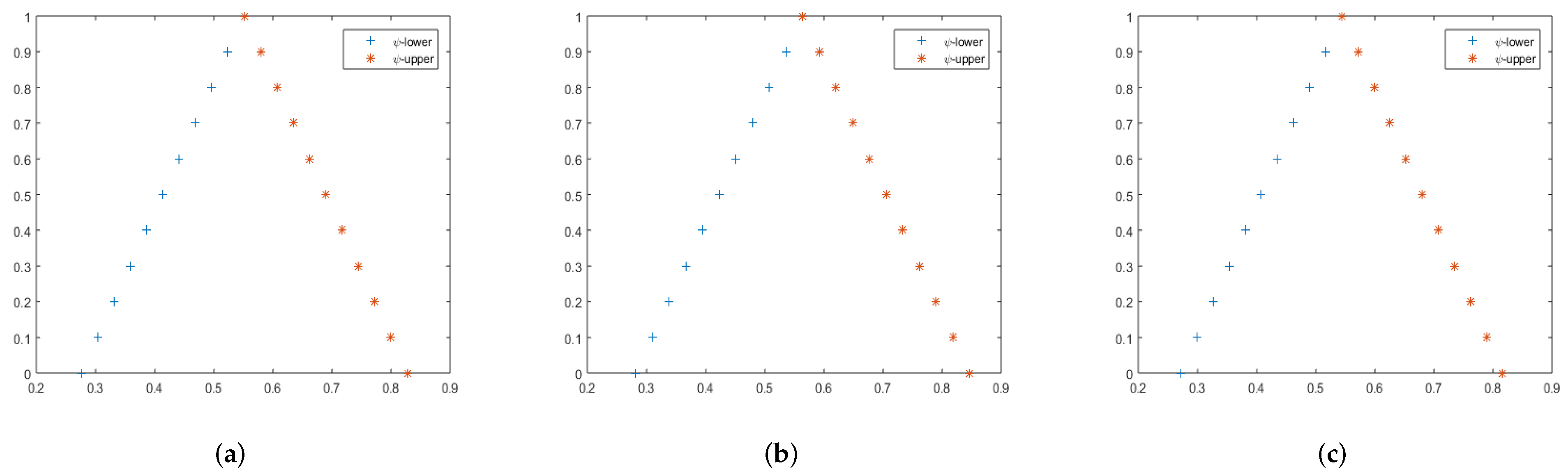
In Figure 5, we plot $2D$ graphs of the approximation solutions for fuzzy fractional wave equations on Cantor set. Figure 5a shows that for $\theta =5,\vartheta =2,n=3,\beta =1.25,1.50,1.75$, the fuzzy fractional wave equation becomes bounded and closed. Moreover, the $\underline{\psi }$ sign shows increasing functions and $\overline{\psi }$ denotes decreasing functions on the $\varrho$-level set of $\psi$. To reflect the concept of the $\varrho$-level set, Figure 5a illustrates that the $\varrho$-level set of the fuzzy fractional wave equation is bounded and closed for $\theta =5$. Similarly, in Figure 5b,c, we can observe the same explanation of the $\varrho$-level set closedness and boundedness for Example 6.

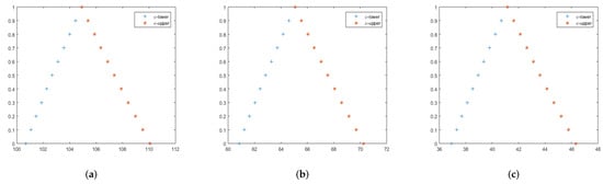
Figure 5. The approximate lower and upper solutions of (167) at (a–c) $\theta =5,\vartheta =2,n=3,\beta =1.25$, 1.50, 1.75, respectively. Moreover, (a–c) are 2D figures for the approximate solutions of the fuzzy fractional wave equation on the Cantor set of $\psi (\vartheta ,\theta )$ in Example 6.

5. Conclusions

In this paper, the hybrid LFFHPSTM, LFFSDM, and LFFSVIM have been used to successfully obtain the solutions of LFFPDEs. Computer-based numerical simulations can clarify the fundamental properties of the physical models given in LFFPDEs. The results demonstrate the efficiency and simplicity of the used technique in identifying LFFPDEs. The originality of this work comes from the fact that the utilized methodology has not recently been used for LFFPDEs. The combination that is used has two features; He’s polynomials are used to decompose nonlinear terms in the first case, while fast convergent series solutions in closed form are produced in the second. Furthermore, the LFHPSTM does not necessitate the calculation of complex Adomian polynomials. The LFFHPM and local fuzzy fractional Sumudu transform method (LFFSTM) can be coupled more quickly and provide better mathematical computations than the LFFHPM. The process of determining a solution demonstrates the efficacy and precision of the proposed method. The LFFSDM offers the solution in the form of a series that, if one exists, quickly converges to the precise solution. It is evident from the findings that the LFFSDM produces very accurate solutions with a minimal number of iterations. Moreover, we have investigated the LFFLIM, LFFSEM, LFFVIM, and LFFADM applied to solving fuzzy diffusion and wave equations defined on Cantor sets with fractal conditions. We show that the LFFVIM utilizing the iteration of the correction local fractional function yields numerous successive approximations. However, the exact solution, which is a local fractional continuous function, is provided by the LFFADM, where these components are local fractional continuous functions. The techniques produce approximate solutions to linear and nonlinear fuzzy fractional differential equations.

References

- Zadeh, L.A. Fuzzy sets. Inf. Control 1965, 8, 338–353. [Google Scholar] [CrossRef]
- Zadeh, L.A. The concept of a linguistic variable and its application to approximate reasoning-I. Inf. Sci. 1975, 8, 199–249. [Google Scholar] [CrossRef]
- Zadeh, L.A. The concept of a linguistic variable and its application to approximate reasoning-II. Inf. Sci. 1975, 8, 301–357. [Google Scholar] [CrossRef]
- Zadeh, L.A. The concept of a linguistic variable and its application to approximate reasoning-III. Inf. Sci. 1975, 9, 43–80. [Google Scholar] [CrossRef]
- Zadeh, L.A. Toward a generalized theory of uncertainty (GTU)—An outline. Inf. Sci. 2005, 172, 1–40. [Google Scholar] [CrossRef]
- Zadeh, L.A. Is there a need for fuzzy logici? Inf. Sci. 2008, 178, 2751–2779. [Google Scholar] [CrossRef]
- Negoita, C.V.; Ralescu, D. Applications of Fuzzy Sets to Systems Analysis; Wiley: New York, NY, USA, 1975. [Google Scholar]
- Aytar, S.; Pehlivan, S. Statistically monotonic and statistically bounded sequences of fuzzy numbers. Inf. Sci. 2006, 176, 734–744. [Google Scholar] [CrossRef]
- Aytar, S. Statistical limit points of sequences of fuzzy numbers. Inf. Sci. 2004, 165, 129–138. [Google Scholar] [CrossRef]
- Osman, M.; Xia, Y. Solving fuzzy fractional q-differential equations via fuzzy q-differential transform. J. Intell. Fuzzy Syst. 2023, 44, 2791–2846. [Google Scholar] [CrossRef]
- Allahviranloo, T.; Ghanbari, B. On the fuzzy fractional differential equation with interval Atangana-Baleanu fractional derivative approach. Chaos Solitons Fractals 2020, 130, 109397. [Google Scholar] [CrossRef]
- Allahviranloo, T.; Gouyandeh, Z.; Armand, A. Fuzzy fractional differential equations under generalized fuzzy Caputo derivative. J. Intell. Fuzzy Syst. 2014, 26, 1481–1490. [Google Scholar] [CrossRef]
- An, T.V.; Hoa, N.V. Fuzzy differential equations with Riemann-Liouville generalized fractional integrable impulses. Fuzzy Sets Syst. 2022, 429, 74–100. [Google Scholar] [CrossRef]
- Agarwal, R.P.; Arshad, S.; O’Regan, D.; Lupulescu, V. Fuzzy frac-tional integral equations under compactness type condition. Fract. Calc. Appl. Anal. 2012, 15, 572–590. [Google Scholar] [CrossRef]
- Alinezhad, M.; Allahviranloo, T. On the Solution of Fuzzy Fractional Optimal Control Problems with the Caputo Derivative. Inf. Sci. 2017, 421, 218–236. [Google Scholar] [CrossRef]
- Dai, R.; Chen, M. The structure stability of periodic solutions for first-order uncertain dynamical systems. Fuzzy Sets Syst. 2020, 400, 134–146. [Google Scholar] [CrossRef]
- Dong, N.P.; Long, H.V.; Giang, N.L. The fuzzy fractional SIQR model of com-puter virus propagation in wireless sensor network using Caputo Atangana-Baleanu derivatives. Fuzzy Sets Syst. 2021, 429, 28–59. [Google Scholar] [CrossRef]
- Long, H.V.; Son, N.T.K.; Tam, H.T.T.; Yao, J.C. Ulam stability for fractional partial integro-differential equation with uncertainty. Acta Math. Vietnam 2017, 42, 675–700. [Google Scholar] [CrossRef]
- Liu, Y.; Zhu, Y.; Lu, Z. On Caputo-Hadamard uncertain fractional differential equations. Chaos Solitons Fractals 2021, 146, 110894. [Google Scholar] [CrossRef]
- Mazandarani, M.; Kamyad, A.V. Modified fractional Euler method for solving fuzzy fractional initial value problem. Commun. Nonlinear Sci. Numer. Simul. 2013, 18, 12–21. [Google Scholar] [CrossRef]
- Mazandarani, M.; Najariyan, M. Type-2 fuzzy fractional derivatives. Commun. Nonlinear Sci. Numer. Simul. 2014, 19, 2354–2372. [Google Scholar] [CrossRef]
- Osman, M.; Xia, Y. Solving fuzzy fractional differential equations with applications. Alex. Eng. J. 2023, 69, 529–559. [Google Scholar] [CrossRef]
- Kolwankar, K.M.; Gangal, A.D. Fractional differentiability of nowhere differentiable functions and dimension. Chaos 1996, 6, 505–513. [Google Scholar] [CrossRef] [PubMed]
- Yang, X.J. Advanced Local Fractional Calculus and Its Applications; World Science: New York, NY, USA, 2012. [Google Scholar]
- Yang, Y.J.; Hua, L.Q. Variational iteration transform method for fractional dif-ferential equations with local fractional derivative. Abs. Appl. Anal. 2014, 9, 760957. [Google Scholar]
- Golmankhaneh, A.K.; Yang, X.J.; Baleanu, D. Einstein field equations within local fractional calculus. Rom. J. Phys. 2015, 60, 22–31. [Google Scholar]
- Yang, X.J.; Baleanu, D.; Zhong, W.P. Approximate solutions for diffusion equations on cantor space-time. Proc. Rom. Acad. Ser. A 2013, 14, 127–133. [Google Scholar]
- Yang, X.J.; Srivastava, H.M.; Cattani, C. Local fractional homotopy perturbation method for solving fractal partial differential equations arising in mathematical physics. Rom. Rep. Phys. 2015, 67, 752–761. [Google Scholar]
- Yang, A.M.; Li, J.; Srivastava, H.M.; Xie, G.N.; Yang, X.J. Local fractional laplace variational iteration method for solving linear partial differential equations with local fractional derivative. Dis. Dyn. Nat. Soc. 2014, 8, 365981. [Google Scholar] [CrossRef]
- Jassim, H.K. Local fractional Laplace decomposition method for nonhomogeneous heat equations arising in fractal heat flow with local fractional derivative. Int. J. Adv. Appl. Math. Mech. 2015, 2, 1–7. [Google Scholar]
- Wang, K. Solitary wave dynamics of the Local fractional Bogoyavlen-sky-Konopelchenko model. Fractals 2023, 31, 2350054. [Google Scholar] [CrossRef]
- Wang, K. New solitary wave solutions for the fractional Jaulent-Miodek Hierarchy model. Fractals 2023, 31, 2350060. [Google Scholar]
- Watugala, G.K. Sumudu transform—A new integral transform to solve differential equations and control engineering problems. Int. J Math. Educ. Sci. Technol. 1998, 24, 35–43. [Google Scholar] [CrossRef]
- Weerakoon, S. Complex inversion formula for Sumudutransform. Int. J. Educ. Math. Sci. Technol. 1998, 29, 618–621. [Google Scholar]
- Asiru, M.A. Sumudu transform and solution of integralequations of convolution type. Int. Educ. Math. Sci. Technol. 2001, 32, 906–910. [Google Scholar] [CrossRef]
- Asiru, M.A. Applications of Sumudu transform to discretedynamic system. Int. J. Educ. Math. Sci. Technol. 2003, 34, 944–949. [Google Scholar] [CrossRef]
- Belgacem, F.M.; Karaballi, A.A. Sumudu transform fundamental properties investigation, applications. J. Appl. Math. Stoch. Anal. 2006, 2006, 91083. [Google Scholar] [CrossRef]
- Osman, M.; Xia, Y.; Omer, O.A.; Hamoud, A. On the fuzzy solution of linear-nonlinear partial differential equations. Mathematics 2022, 10, 2295. [Google Scholar] [CrossRef]
- Osman, M.; Gong, Z.T.; Mustafa, A.M.; Yong, H. Solving fuzzy (1 + n)-dimensional Burgers’ equation. Adv. Differ. Equ. 2021, 219, 219. [Google Scholar] [CrossRef]
- Osman, M.; Gong, Z.T.; Mustafa, A.M. Comparison of fuzzy Adomian decomposition method with fuzzy VIM for solving fuzzy heat-like and wave-like equations with variable coefficients. Adv. Differ. Equ. 2020, 327, 327. [Google Scholar] [CrossRef]
- Osman, M.; Almahi, A.; Omer, O.A.; Mustafa, A.M.; Altaie, S.A. Approximation solution for fuzzy fractional-order partial differential equations. Fractal Fract. 2022, 6, 646. [Google Scholar] [CrossRef]
- Osman, M.; Xia, Y.; Marwan, M.; Omer, O.A. Novel Approaches for solving fuzzy fractional partial differential equations. Fractal Fract. 2022, 6, 656. [Google Scholar] [CrossRef]
- Patela, T.; Meher, R. A Study on Temperature Distribution, Efficiency and Effectiveness of longitudinal porous fins by using Adomian Decomposition Sumudu Transform Method. Procedia Eng. 2015, 127, 751–758. [Google Scholar] [CrossRef]
- Saadeh, R.; Ahmed, S.A.; Qazza, A.; Elzaki, T.M. Adapting partial differential equations via the modified double ARA-Sumudu decomposition method. Partial. Differ. Equ. Appl. Math. 2023, 8, 100539. [Google Scholar] [CrossRef]
- He, J.H. Approximate solution of nonlinear differential equations with convolution product nonlinearities. Comput. Methods Appl. Mech. Eng. 1998, 167, 69–73. [Google Scholar] [CrossRef]
- He, J.H. Variational iteration method for autonomous ordinary differential systems. Appl. Math. Comput. 2000, 114, 115–123. [Google Scholar] [CrossRef]
- Shah, N.A.; Dassios, I.; El-Zahar, E.R.; Chung, J.D.; Taherifar, S. The Variational It-eration Transform Method for Solving the Time-Fractional Fornberg-Whitham Equation and Comparison with Decomposition Transform Method. Mathematics 2021, 9, 141. [Google Scholar] [CrossRef]
- Singh, G.; Singh, I. Semi-analytical solutions of three-dimensional (3D) coupled Burgers’ equations by new Laplace variational iteration method. Part. Differ. Equ. Appl. Math. 2022, 6, 100438. [Google Scholar] [CrossRef]
- Prakasha, A.; Kumar, M.; Baleanu, D. A new iterative technique for a fractional model of nonlinear Zakharov-Kuznetsov equations via Sumudu transform. Appl. Math. Comput. 2018, 334, 30–40. [Google Scholar] [CrossRef]
- Anac, H.; Merdan, M.; Kesemen, T. Solving for the random component time-fractional partial diferential equations with the new Sumudu transform iterative method. SN Appl. Sci. 2020, 2, 1112. [Google Scholar] [CrossRef]
- Bhargava, A.; Jain, D.; Suthar, D.L. Applications of the Laplace variational iteration method to fractional heat like equations. Partial. Differ. Equ. Appl. Math. 2023, 8, 100540. [Google Scholar] [CrossRef]
- Nadeem, M.; Li, F.; Ahmad, H. Modified Laplace variational iteration method for solving fourth-order parabolic partial differential equation with variable coefficients. Comput. Math. Appl. 2019, 78, 2052–2062. [Google Scholar] [CrossRef]
- Zhang, Y.; Cattani, C.; Yang, X.J. Local fractional homotopy perturbation method for solving non-homogeneous heat conduction equations in fractal domains. Entropy 2015, 17, 6753–6764. [Google Scholar] [CrossRef]
- Singh, J.; Kumar, D.; Nieto, J.J. A reliable algorithm for a local fractional tricomi equation arising in fractal transonic flow. Entropy 2016, 18, 206. [Google Scholar] [CrossRef]
- Zhao, D.; Singh, J.; Kumar, D.; Rathore, S.; Yang, X.J. An efficient computational technique for local fractional heat conduction equations in fractal media. J. Nonlinear Sci. Appl. 2017, 10, 1478–1486. [Google Scholar] [CrossRef]
- Kumar, D.; Tchier, F.; Singh, J.; Baleanu, D. An efficient computational technique for fractal vehicular traffic flow. Entropy 2018, 20, 259. [Google Scholar] [CrossRef]
- Prakash, A.; Kaur, H. An efficient hybrid computational technique for solving nonlinear local fractional partial differential equations arising in fractal media. Nonlinear Eng. 2018, 7, 229–235. [Google Scholar] [CrossRef]
- Dubey, V.P.; Singh, J.; Alshehri, A.M.; Dubey, S.; Kumar, D. A comparative analysis of two computational schemes for solving local fractional Laplace equations. Math. Meth. Appl. Sci. 2021, 44, 13540–13559. [Google Scholar] [CrossRef]
- Srivastava, H.M.; Golmankhaneh, A.K.; Baleanu, D.; Yang, X.J. Local fractional Sumudu transform with application to IVPs on Cantor sets. Abstr. Appl. Anal. 2014, 2014, 620529. [Google Scholar] [CrossRef]
- Rivaz, A.; Fard, O.S.; Bidgoli, T.A. Solving fuzzy fractional differential equations by generalized differential transform method. SeMA J. 2016, 73, 149–170. [Google Scholar] [CrossRef]
- Kaleva, O. Fuzzy differential equations. Fuzzy Sets Syst. 1987, 24, 301–317. [Google Scholar] [CrossRef]
- Wu, C.; Gong, Z. On Henstock integral of fuzzy-number-valued functions (1). Fuzzy Sets Syst. 2001, 120, 523–532. [Google Scholar] [CrossRef]
- Yang, H.; Gong, Z. I11-Posedness for fuzzy Fredholm integral equations of the first kind and regularization methods. Fuzzy Sets Syst. 2019, 358, 132–149. [Google Scholar] [CrossRef]
- Bede, B.; Stefanini, L. Generalized differentiability of fuzzy-valued functions. Fuzzy Sets Syst. 2013, 230, 119–141. [Google Scholar] [CrossRef]
- Bede, B.; Gal, S.G. Generalizations of the differentiable fuzzy number valued functions with applications to fuzzy differential equations. Fuzzy Sets Syst. 2005, 151, 581–599. [Google Scholar] [CrossRef]
- Allahviranloo, T.; Gouyandeha, Z.; Armanda, A.; Hasanoglub, A. On fuzzy solutions for heat equation based on generalized Hukuhara differentiability. Fuzzy Sets Syst. 2015, 265, 1–23. [Google Scholar] [CrossRef]
- Salahshour, S.; Allahviranloo, T.; Abbasbandy, S. Solving fuzzy fractional differential equa-tions by fuzzy Laplace transforms. Commun. Nonlinear Sci. Numer. Simul. 2012, 17, 1372–1381. [Google Scholar] [CrossRef]
- Yang, X.J. Local Fractional Functional Analysis and Its Applications; Asian Academic: Hong Kong, China, 2011. [Google Scholar]
- Ziane, D.; Baleanu, D.; Belghaba, K.; Cherif, M. Local fractional Sumudu decomposition method for linear partial differential equations with local fractional derivative. J. King Saud. Univ. Sci. 2019, 31, 83–88. [Google Scholar] [CrossRef]
- Hu, M.S.; Agarwal, R.P.; Yang, X.J. Local fractional Fourier series with application to wave equation in fractal vibrating string. Abstr. Appl. Anal. 2012, 2012, 567401. [Google Scholar] [CrossRef]
Disclaimer/Publisher’s Note: The statements, opinions and data contained in all publications are solely those of the individual author(s) and contributor(s) and not of MDPI and/or the editor(s). MDPI and/or the editor(s) disclaim responsibility for any injury to people or property resulting from any ideas, methods, instructions or products referred to in the content. |
© 2023 by the authors. Licensee MDPI, Basel, Switzerland. This article is an open access article distributed under the terms and conditions of the Creative Commons Attribution (CC BY) license (https://creativecommons.org/licenses/by/4.0/).