Abstract
A reduced power system’s inertia represents a big issue for high penetration levels of renewable generation sources. Recently, load frequency controllers (LFCs) and their design have become crucial factors for stability and supply reliability. Thence, a new optimized multiloop fractional LFC scheme is provided in this paper. The proposed multiloop LFC scheme presents a two-degree-of-freedom (2DOF) structure using the tilt–integral–derivatives with filter (TIDN) in the first stage and the tilt–derivative with filter (TDN) in the second stage. The employment of two different loops achieves better disturbance rejection capability using the proposed 2DOF TIDN-TDN controller. The proposed 2DOF TIDN-TDN method is optimally designed using the recent powerful marine predator optimizer algorithm (MPA). The proposed design method eliminates the need for precise modeling of power systems, complex control design theories, and complex disturbance observers and filter circuits. A multisourced two-area interlinked power grid is employed as a case study in this paper by incorporating renewable generation with multifunctionality electric vehicle (EV) control and contribution within the vehicle-to-grid (V2G) concept. The proposed 2DOF TIDN-TDN LFC is compared with feature-related LFCs from the literature, such as TID, FOTID, and TID-FOPIDN controllers. Better mitigated frequency and tie-line power fluctuations, faster response, lower overshot/undershot values, and shorter settling time are the proven features of the proposed 2DOF TIDN-TDN LFC method.
Keywords:
electrical grid; electric vehicle application; fractional order control theory; load frequency controller (LFC); marine predator optimizer (MPA); multisourced power systems; renewable power sources; vehicle to grid (V2G) MSC:
68N30
1. Introduction
1.1. Overview
Advancements in energy transition have led to the widespread installation of renewable energy sources (RESs) [1]. In addition, wide global plans have been set to continue reducing carbon emissions in the environment. Another key factor for the energy transition is the wide replacement of various conventional fuel-based vehicles by clean electric vehicles (EVs) [2]. In addition, EVs and their charging infrastructures can widely contribute to improving electrical power system performance by controlling their charging/discharging commands, times, and power flows. However, the installed RESs at high levels of penetration and the installed EVs in power grids have led to different characteristics of modern power systems. Additionally, special attention must be paid to designing their associated control systems. The proper design and implementation of control methods have improved performance in several applications, such as unmanned aerial vehicles (UAVs) [3,4], networked mobile robots [5], nonholonomic vehicles [6,7], etc.
The structure of RESs is different from synchronous generator-based conventional electrical generation systems. They are based on power electronics conversion systems (PECSs) for grid integration. However, PECSs-based renewable generation systems lack inertia, and hence, deteriorated power system stability exists in modern electrical power systems [8]. This is due to the low stored mechanical power in power systems’ inertia. This mechanical power helps retain system stability and operation during transients of generation, loading, and faults [9]. Thence, high levels of RESs penetration result in stability concerns in power grids. The load frequency controllers (LFCs) have shown great ability to regulate power grids’ frequencies and tie-line powers between areas during normal conditions, as well as abnormal operating conditions [10]. Load frequency controllers (LFCs) regulate both the power output from generation sources and the loading demands, hence the enhanced regulation of the frequency signals besides the tie-line powers among areas [11,12,13].
1.2. Literature Review
The existing LFC methods in the literature can be mainly classified according to the controller type and number of loops. Based on the LFC type, several control methods have been introduced, such as integer-order control (IO) [14], fractional-order control (FO), sliding mode controllers (SMCs) [15], SMC with interval-type-2 fuzzy [16], repetitive control [17], model predictive controls (MPCs) [18,19], robust control [20,21], machine and deep learning (ML and DL) [22,23], etc. Additionally, based on the number of loops, various degrees of freedom (DOF) have been introduced, such as single-DOF (1DOF), two-DOF (2DOF), and three-DOF (3DOF) [24]. In 1DOF, area control error signals (ACEs) are used in the control feedback loop, whereas in 2DOF, another feedforward loop is added based on the frequency deviation signal with the ACE feedback loop. In 3DOF, a third feedforward signal is used based on the tie-line power between areas. Moreover, a variety of metaheuristic-based optimization methods has been introduced for optimally designing various control parameters in a simultaneous way [25,26]. The optimizer algorithms can be coupled with LFC methods to enhance the power system response and performance regarding the frequency with tie-line power regulations.
Several combinations of IO and FO LFC schemes have been extensively provided in the literature in different single and multi-area-based power systems [27,28]. For instance, the IO-based integrator (I), proportional–integrator (PI), and proportional–integrator–derivative (PID) control schemes represent the most widely introduced LFC methods. An optimum PI LFC has been proposed in [29]. Optimization procedures have been achieved using the binary moths–flame optimization (MFO). Another hybrid gravitation search with a firefly algorithm (hGFA)-based optimized PI LFC has been proposed in [30]. Further optimum PI LFC methods have been proposed using Harris Hawks optimizer algorithm (HHO) [31], and gray wolf optimization (GWO) [32]. Additionally, the PID has been provided in the literature for achieving LFC, such as in [33], by using a hybrid improved gravitation search algorithm and binary particle swarm optimizer (IGSA-BPSO). Optimum PID LFC methods were introduced using artificial bees colony (ABC) in [34] and stability boundary locus (SBL) optimizer in [35]. The applications of the I, ID, and PID integer-order LFCs have been presented and compared in [36]. The salp swarm optimization algorithm (SSA), grasshopper optimizer algorithm (GOA), and collective decision optimizer algorithm (CDO) have been presented for the optimum design of compared controllers. Another PI event-triggered LFC has been presented in [37], wherein it achieved lower peak overshoot/undershoot peaks compared with existing controllers. An optimized PID LFC method has been presented in [38] using a hybrid algorithm of sparrow searching and gray wolf optimization (SSAGWO). The above-presented literature is based on 1DOF control structures, and they are shown to be simple, easily designed, and implementable using low-cost processors, etc. However, in modern power grids, nonlinearities and uncertainties due to RESs hinder their superiority.
Additional flexibility has been achieved through using the FO control structures in LFC [39]. The FO terms are combined to form various structures using the FO tilt (T), FO integrator (), FO derivative (), and FO-based filter. A comparison between IO and FO LFC has been presented in [40] verifying that FO LFC has more flexibility. The results verify that FOPID has a faster response and better damping than the IO-based PID LFC scheme. For instance, FOPID has been proposed in [41], while its optimization procedures have been made using the movable damped waves optimizer (MDWA). Moreover, the sine–cosine optimizer algorithm (SCA) has been presented for FOPID optimization in [42]. The tilt FO control has also been presented in the literature for LFC [43]. The ABC optimization [44], pathfinder algorithm (PFA) [45], and differential evolutions algorithms (DEs) [43] were provided in the literature for optimizing tilt-based LFC methods. As an extension for FO control, several combinations have been provided and verified in literature work. The combination leads to the added benefits of both control methods. For instance, TID has been combined with FOPID in [46] to form a hybrid TFOID controller. The optimization processes were achieved through using the artificial ecosystem optimizer (AEO) algorithm. An extended hybrid TFOID with FO filter has been presented in [47] using an artificial hummingbird optimization algorithm (AHA).
From another perspective, various high-DOF LFC methods have been proposed in the literature. A 2DOF PID control has been presented in [48] for LFC. The flower pollination optimizer algorithm (FPA) was presented in [49] for optimizing a 2DOF PID controller. In [50], a 2DOF PID was proposed, and it is optimized through the dragonfly optimizer algorithm (DA) through the development of a new integral based on the weighted goals fitness functions (IB-WGFF). In [51], a 2DOF PD-PID controller has been proposed. A 2DOF PI-PID has been provided in [52], wherein the optimization process is achieved through a slap swarm optimization algorithm (SSA). In addition, a 3DOF (1 + PD)-PID LFC method has been provided in [53], in which an African vulture optimizer algorithm (AVOA) has been introduced for optimizing the controller parameters. A 2DOF TIDF LFC method was provided in [54] with the whale optimizer algorithm (WOA) for design optimization. A higher DOF has been proven to offer superior operation and transient performance of LFC compared with 1DOF-based controllers. Therefore, the focus of this paper is to develop a new 2DOF LFC method using the fractional-order control theory. In addition, optimized parameters are designed using the recent powerful marine predator optimizer algorithm (MPA).
1.3. Article Contribution
Existing work in the literature proves that increasing the DOF of the LFC method can lead to better performance and mitigation of expected disturbances in modern power grids. In addition, selecting a proper optimization algorithm jointly with the proposed controller can achieve enhanced selection processes of the optimized parameters. Moreover, future modern power grids are expected to be more volatile and less stable due to the reduced inertia resulting from the extensive use of PECSs. Among the existing optimization algorithms, the MPA-based optimization algorithm has achieved improved performance in several optimum values searching problems [55,56]. Some featured applications include maximum power extraction [57], PV model parameters extraction [58], PV array reconfiguration [59], PID-based LFC [60], and FO-based LFC methods [61,62].
Therefore, the authors of this paper were motivated to present an MPA-based optimization of the newly proposed 2DOF TIDN-TDN LFC method. The main contribution points in this article are as follows:
- A higher degree of freedom FO-based LFC method is proposed. The newly proposed controller is based on developing a multiloop two-degrees-of-freedom (2DOF) fractional-order-based LFC method. The proposed 2DOF LFC method uses the tilt–integral–derivatives with filter (TIDN) in the outer loop and the tilt–derivative with filter (TDN) in the inner loop.
- The proposed TIDN-TDN controller includes high flexibility due to its included FO operators, which help with better optimization of control performance. The proposed TIDN-TDN controller represents a new combination of fractional-order-based LFC compared with existing control structures in the literature.
- The improved performance using the proposed TIDN-TDN controller results from employing a feedback signal in the outer loop using ACE signal to mitigate the low-frequency fluctuations. Furthermore, the proposed 2DOF TIDN-TDN LFC method employs a feedforward loop using the frequency deviation signal to mitigate the high-frequency disturbances. Thence, better disturbance rejection capability is obtained using the proposed 2DOF TIDN-TDN controller. Moreover, the proposed TIDN-TDN LFC method does not require additional components and/or observer design and/or filter elements.
- An effective control and coordination method is proposed to control the participation of installed and future EVs using the TID controller and is coordinated with the proposed 2DOF TIDN-TDN LFC method. Accordingly, the installed EVs in future modern power systems participate in an effective way to dampen existing disturbances by utilizing the inherent EV batteries. This, in turn, leads to better EV utilization in future power systems with the expected continuous replacements of EVs. The coordination process is achieved inherently within the proposed controller and its design optimization method.
- An improved optimized design of the proposed 2DOF TIDN-TDN LFC method and EV TID controller is presented in this paper using the recent powerful marine predator optimizer algorithm (MPA) method. The parameters of the proposed controllers are determined simultaneously in all the studied interconnected power grids. The proposed method eliminates the need for complex control theories and/or mathematical determination processes using classical control methods. Thence, complex control designs and modeling are avoided using the powerful MPA optimizer.
- Further improvements are achieved by the proposed controller by avoiding the common problems of disturbance observer-based control, such as precise model dependency, complex tuning and design requirements, high computational complexity, sensitivity to measurement noise, and limited applicability.
In this work, the practical characteristics of connected renewable energy sources, grid battery contribution, and grid model parameter variations are considered. However, for a more practical extension of this work, the interference between voltage and frequency control designs must be considered. In addition, the effects of existing communication delays in power systems must be modeled and considered, especially with the move toward smarter power grid trends.
The remaining sections in this article are organized as follows: The detailed modeling, mathematical representation, and components of the selected power grid are presented in Section 2. The existing LFCs from the literature are presented in Section 3 with the FO control theory. The proposed 2DOF TIDN-TDN is introduced in Section 4. The design optimization and the MPA optimizer are detailed in Section 5. The obtained simulation results of the 2DOF TIDN-TDN and the selected case study are proven in Section 6 with comparative results. This paper’s conclusions are provided in Section 7.
2. Mathematical Models of the System
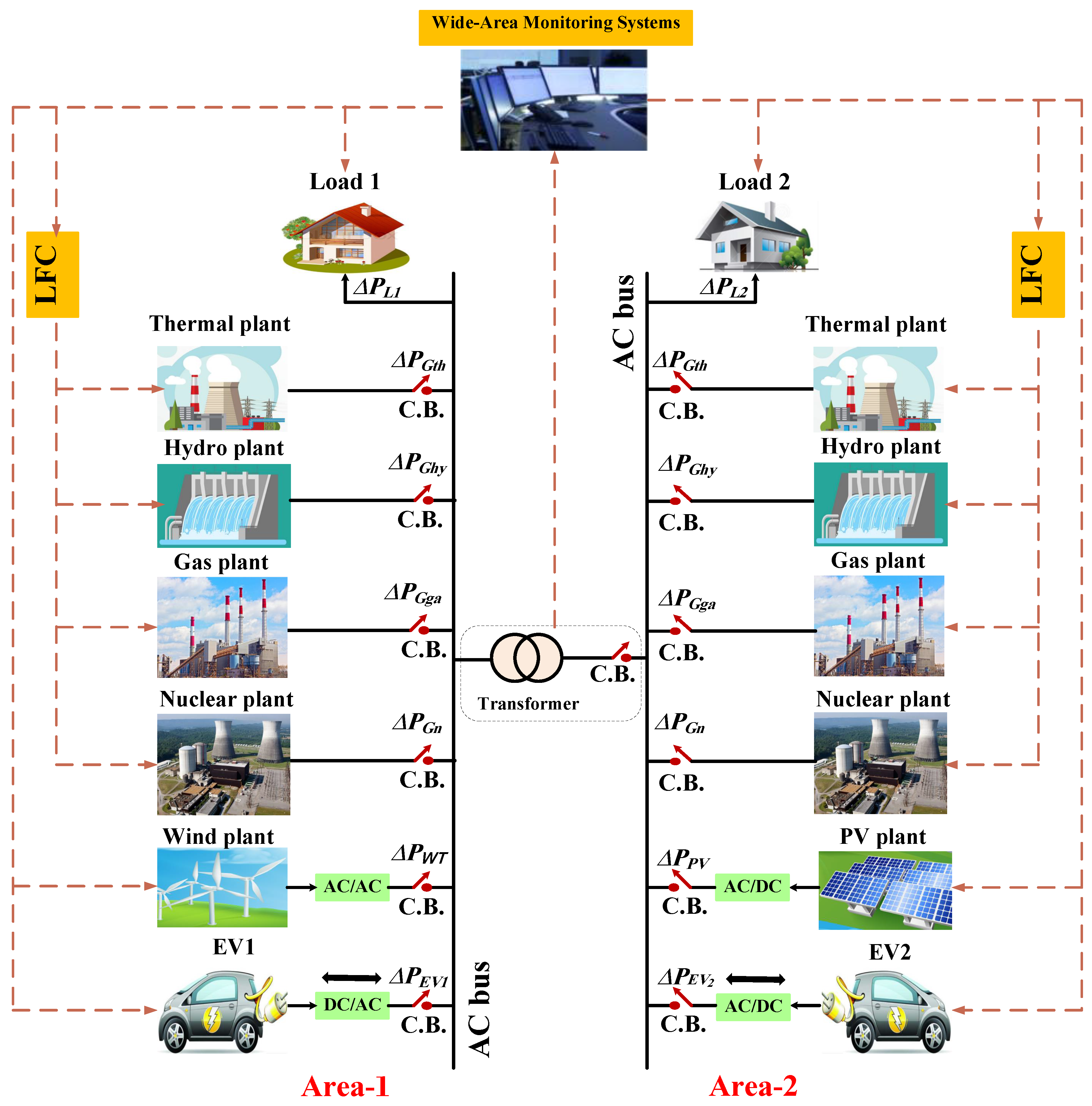
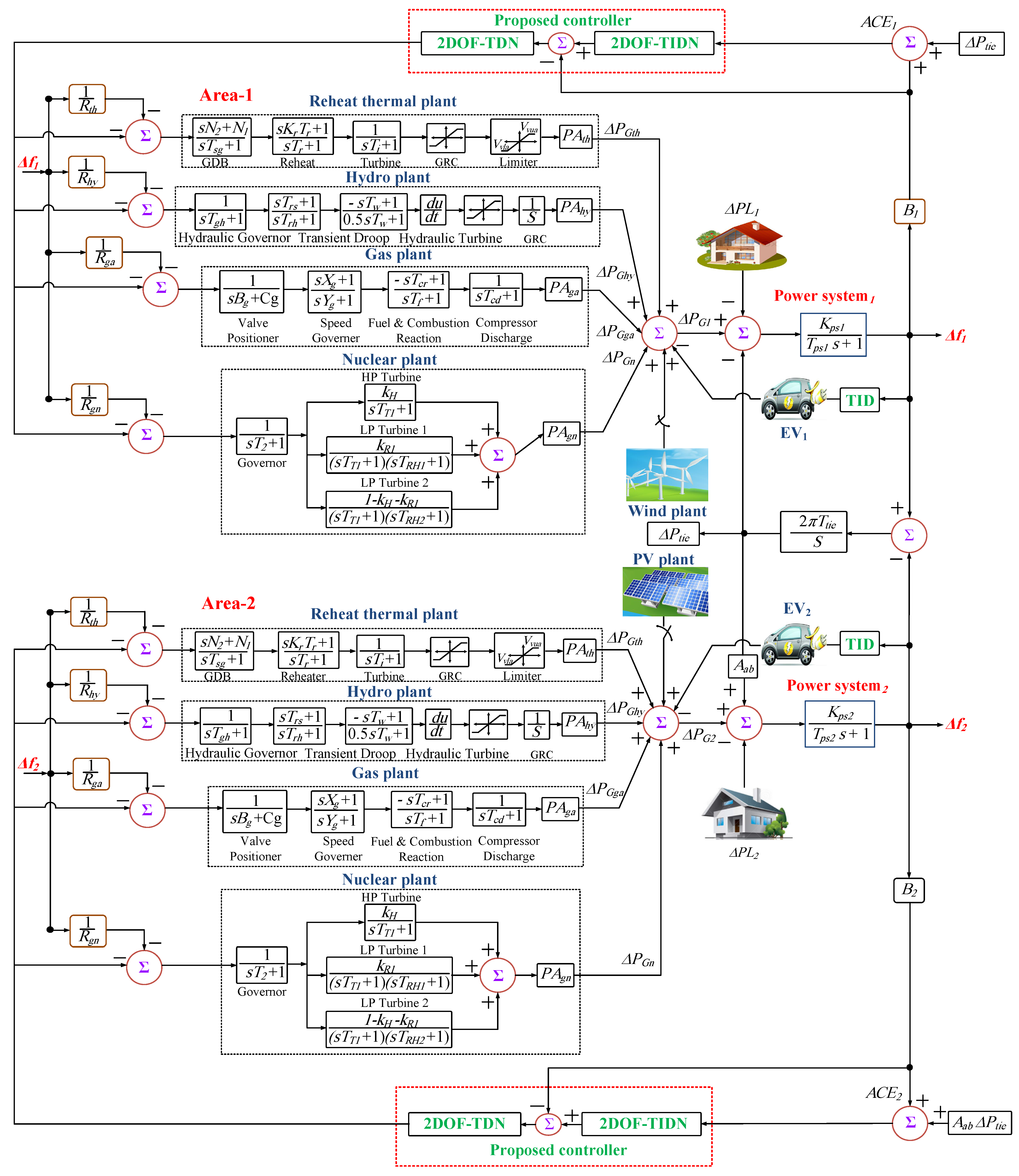
This study focuses on a hybrid power system consisting of two interlinked areas connected via an AC bus tie-line system, as shown in Figure 1. As detailed in Figure 2, each of the two areas features four types of dynamic energy sources: a reheat-based thermal plant, a hydraulics plant, a gas power unit, and a nuclear plant. The physical power systems’ boundaries, such as the generation rate constraints (GRCs) and governors’ dead band (GDB), are modeled and considered as system nonlinearity. Additionally, RESs have a wind unit in area 1 and a PV unit in area 2, and both areas are considering the participation of EVs to control frequency, as depicted in Figure 2. Each area in the system being studied is equipped with a frequency controller that regulates the power output from various energy units. To have control of the power injected by EVs and to take part in frequency regulations within studied areas, another controller is added. In the system under study, each area possesses a rated capacity of 2000 MW, and its nominal loading is 1740 MW. The system parameters for the system under study are shown in the Appendix A section of this paper.

Figure 1.
Power system structure of the two studied areas.
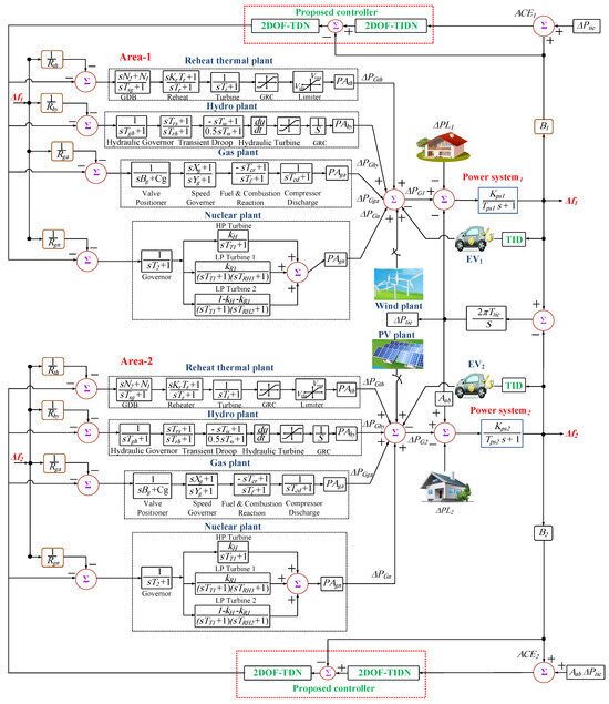
Figure 2.
Mathematical model details of the studied diverse-source two-area interlinked power systems with EVs and RESs.
2.1. Modeling Various Generation Sources
2.1.1. Thermal Plant
The first-order transfer function is used to model reheating using the work in [63] as follows:
where is the gain of the steam turbine, and is its time constant, whereas represents the time constant of the reheater transfer function. The symbol s denotes the Laplace transform s-domain. The model includes thermal units governed by generation rate constraints GRC and GDB, with the GRCs set at 10% pu/min for both increasing and decreasing scenarios (0.0017 pu·MW/s). With respect to the change in addition to its rate for speed, a linearized version for modeling GDB can be utilized. The Fourier series was utilized to create the GDB transfer function model with a 0.5 percent for backlash as follows:
where and denote Fourier coefficients selected as = 0.8 and = −0.2/, as presented in [64].
2.1.2. Hydraulic Plant
The governor, droop compensations, and the penstock turbine make up the Hydraulic turbine’s general transfer function. In [46], it can be shown as follows:
The considered GRCs for the hydraulic plant represented as increasing/decreasing rates are 270% pu/min (0.045 pu·MW/s) and 360% pu/min (0.06 pu·MW/s), respectively.
2.1.3. Gas Plant
The general transfer function of the gas turbine comprises components such as the valve positioner, speed governor, combustion reactions and fuel, and the compressor’s discharge. In [63], it can be shown as follows:
where, , , , , , , and denote the valve positioner’s time constant, valve position of the gas turbine, the time constant of lead, the time constant of lag for the gas turbine, the time delay of a gas turbine’s combustion reactions, the time constant of gas turbine fuel, and the time constant of the compressor’s discharge volume, respectively.
2.1.4. Nuclear Plant
The model for the nuclear plant, as detailed in [65], comprises a speed governor, a high-pressure type turbine, and two low-pressure-type turbines. It is represented as follows:
where, , , , and denote the time constant of the speed governor, the high-pressure (HP)-based turbine, first low-pressure (LP) turbine, and second LP turbine, respectively. Also, and denote the gain of the HP-type turbine and the first LP-type turbine’s gain, respectively.
2.2. Modeling Various Renewable Generation Sources
2.2.1. PV Generation
Photovoltaic (PV) generation systems include solar modules, DC/DC converters, DC/AC inverters, and other electrical equipment. Solar modules capture solar energy in DC form, DC/DC converters boost the PV voltage to maximize power extraction, and DC/AC inverters convert the DC voltage into AC for the grid integration process. The PV’s transfer function is provided as follows [46]:
where and denote the gain and time constant of PV plant transfer function. It is assumed that the MPPT controller operates effectively and that all available power from the sun is injected into the power grid, with variations in the solar irradiance and temperature values.
2.2.2. Wind Generation
The amount of power a wind turbine depends on the wind’s velocity at any given moment. The wind turbine system (WTS) determines the pitch angles and creates nonlinearities in the system based on wind speed. The WTS transfer function is provided as follows [46]:
where and denote the gain and time constant of the WTS plant transfer function. The wind power generator is assumed to have excellent tracking of its maximum power available in the wind, and hence, all its available power is injected into the power grid. Also, the faults in the system in addition to degradation effects are neglected in this work.
2.3. Modeling of EVs
The batteries of current EVs can be used to effectively control the power system’s performance. They can be charged or discharged, depending on the power systems’ management controller. These batteries have the potential to improve the power system’s dynamic response, overall effectiveness, and reliability. Figure 3 shows the utilized dynamic modeling representation for the connected EVs in the power system. It is the equivalent electrical circuit modeling, as shown in [46]. In this study, it is assumed that the distribution of EVs among the two connected areas is equal. The proposed system also makes use of connected EVs to help at lowering frequency fluctuation values. The EV model is expressed as follows [46]:
where is the open-circuit voltage for a particular state of charge (), is nominal voltage, and is nominal EV battery capacity (in Ah). Moreover, S is the sensitivity parameter among and . R, F, and T are the gaseous constant, Faraday’s constant, and the temperature, respectively. The degradation and its associated problems in EV batteries are not considered in this work. In addition, it is assumed there is a perfect battery management controller between battery cells, and hence, their SOCs are always balanced.
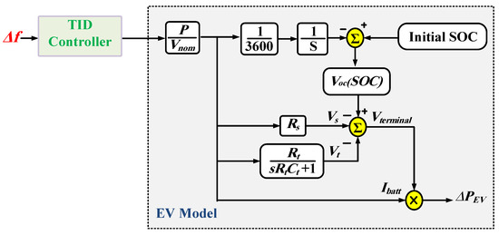
Figure 3.
Dynamic modelling of EVs for the intended LFC study.
3. FO Control Theory and Existing LFCs in Literature
3.1. Existing IO LFC Methods
In the literature, IO-based LFC methods have found wide applications. These methods have demonstrated both enhanced performance and simplified control schemes in various industrial applications. As clarified in the literature review, the I, PI, and PID controllers represent the widely studied IO LFC schemes. Furthermore, various metaheuristic optimization techniques are used for determining optimum LFC parameters. The various gain parameters can be optimally tuned for achieving various objectives, such as controlling rise times, transient times, peaks overshoot/undershoot values, stability criteria, steady-state error, etc. The representations of IO-based LFC methods are as follows:
3.2. FO Control Theory
The FO-based control theories have proven to offer more flexibility and enhanced performance compared with their IO-based counterparts. The FO operators and calculus can be represented using Grunwald–Letnikov, Caputo, and Riemann–Liouville models. The Grundwald–Letnikov scheme represents the derivative using the function (f) within the range a to t limits as follows:
where h is sample time, and the operator is only integer values in (16). Additionally, n is employed to achieve ( and ). These binomials coefficients are determined using
where
Riemann and Liouville defined the FO derivative avoiding the use of sums and limits. Instead, the IO derivative is used and represented as follows:
Another representation of the FO derivative was made by Caputo, and it is defined as follows:
However, can take different forms, as follows:
On the other hand, Oustaloup-based recursive approximations (ORAs) have found wide use in implementing FO derivatives. They are a suitable way for real-time-based digital implementations. They are also a familiar and suitable option for the optimum tuning process of various FO controllers. Thence, ORA-based implementations are employed in this work due to being dominant. The approximation of the mathematical representations of th FO derivatives () is expressed as follows:
where and are poles-zeros locations in , respectively. They are calculated as follows:
where the approximate function has poles/zeros. In addition, N determines the ORA filter’s order within . In this work, ORA representation is utilized with inside the range (), which is selected between rad/s.
3.3. Existing FO LFCs Methods
Additionally, IO-based LFCs have been extended by using their FO-based controllers. The FOPI, TID, and FOPID have been applied to LFCs. For instance, the TID represents a simplified version of the FOPID controller. In the TID controller, a tilted proportional gain, denoted as (), replaces the conventional proportional gain () used in IO-based PID controllers. In this case, the block is referred to as a tilt compensator, and n is called a tilt parameter.
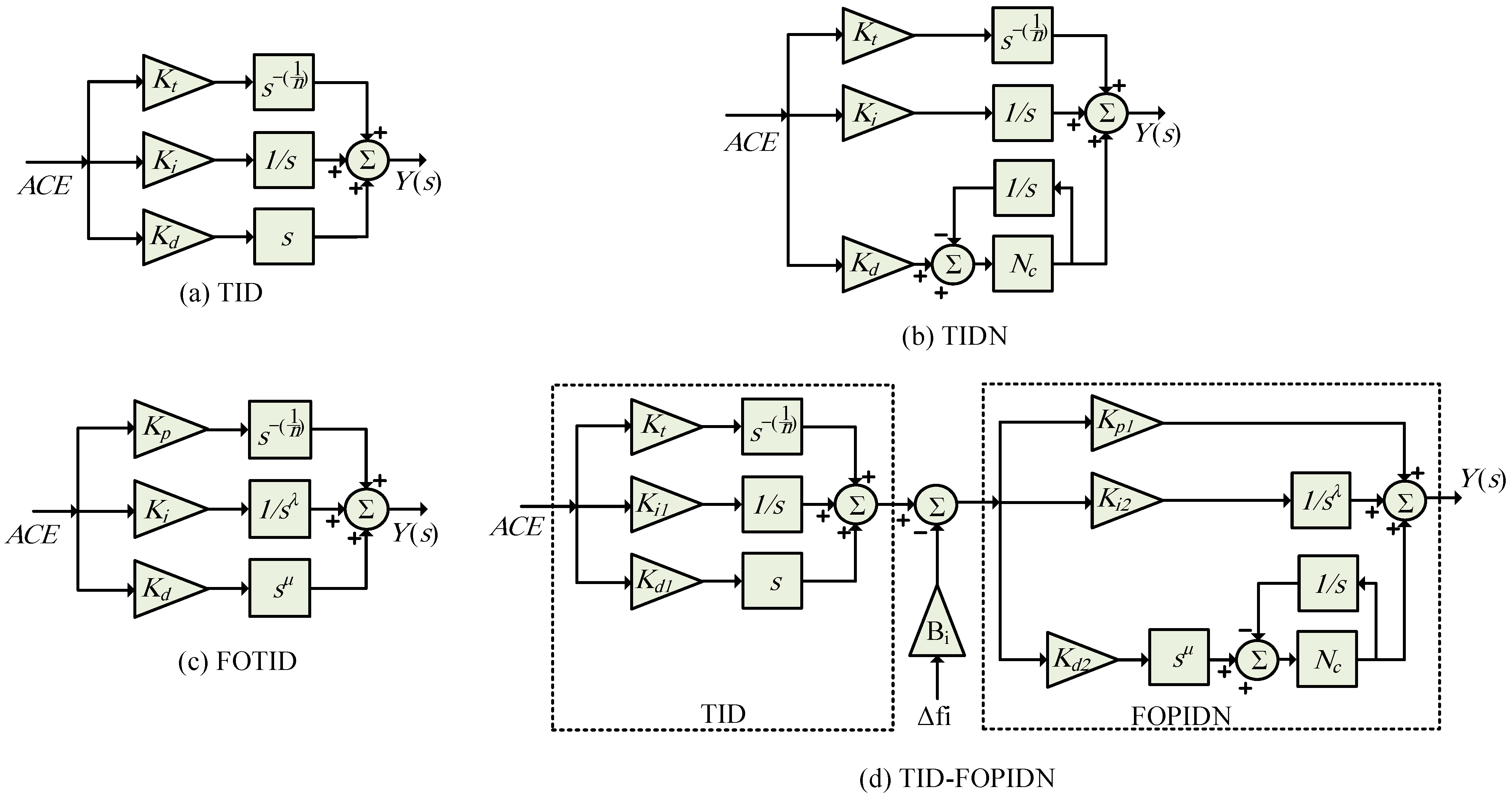
On the other side, the filtering component is added to the derivative component to reduce the chattering noise in the input signal at extreme frequencies. Therefore, the TIDN is used in the literature to improve system stability [46,66]. In the literature, there several studies on integrating one or more IO and/or FO controllers. For instance, FOPID and TID have been integrated to form the FOTID controller (TID). This, in turn, provides more flexibility and helps reduce the settling time of the system during disturbances [46,67]. The block diagrams of the TID, TIDN, FOTID, and TID-FOPIDN controllers [45,63,64] are shown in Figure 4. The featured FO LFC methods can be represented as follows:
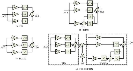
Figure 4.
Block diagrams for some selective FO LFC methods.
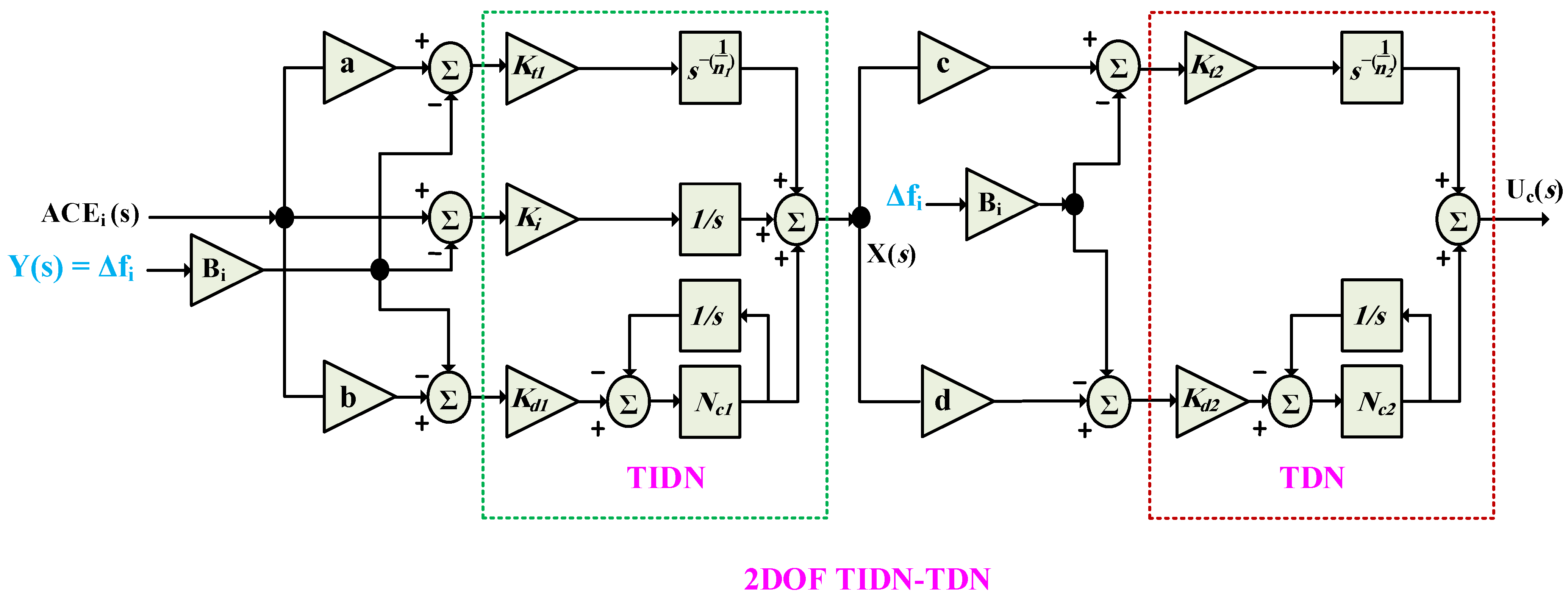
4. The Proposed 2DOF TIDN-TDN Controller
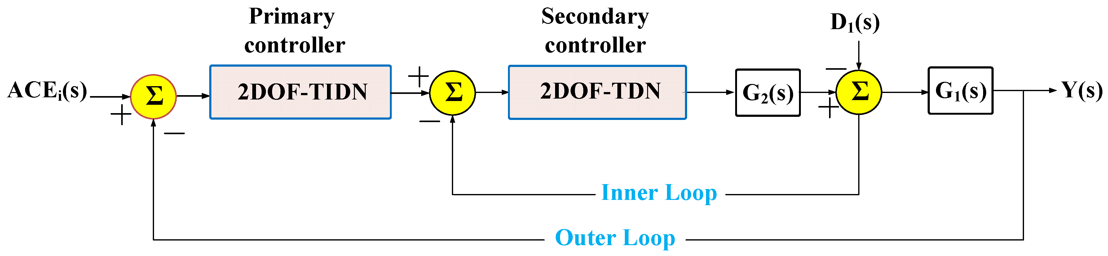
This study introduces a new configuration for LFC applications, featuring a 2DOF multiloop tilt–integral–derivative filtered controller in cascade with a tilt–derivative filtered controller, termed 2DOF TIDN-TDN. The proposed controller is robust enough to allow the flexible management of an intricately reconstructed system by drastically reducing undershoot/overshoot and improving settling time. This controller also has two degrees of freedom, which improves dynamic response by using both the corresponding area frequency deviation () and the area control error () signal as inputs. The schematic structure of the proposed cascaded 2DOF TIDN-TDN controller is shown in Figure 5, in which the TIDN controller serves as the outer controller and the TDN controller serves as the inner controller . Figure 6 details the elements of the proposed cascaded 2DOF TIDN-TDN controller. Utilizing the frequency deviation signals leads to mitigating the existing high-frequency disturbances, while utilizing the ACE loop leads to mitigating the existing low-frequency disturbances. Hence, the proposed 2DOF TIDN-TDN controller provides better rejection of exiting disturbances due to its high DOF. The proposed multiloop controller is represented mathematically as follows:
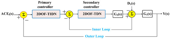
Figure 5.
Proposed multiloop cascaded control structure.
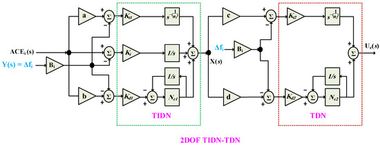
Figure 6.
The proposed cascaded 2DOF TIDN-TDN control structure for LFC in each area.
5. The Process for Obtaining Optimized Control Parameters
5.1. Optimization Process
The two main goals of LFCs are to keep tie-line power fluctuations at their minimum value and to cancel out frequency drifts when there are disturbances in the system. To accomplish the goals in the proposed optimization problem targeting LFC applications, an objective function has to be formulated based on these objectives. The objective function, which combines frequency deviations and tie-line power deviations, has been accumulated by utilizing a variety of widely applied error functions. In this work, four different cost functions were used for optimization processes for the proposed 2DOF TIDN-TDN controller. The four objective functions are represented as follows:
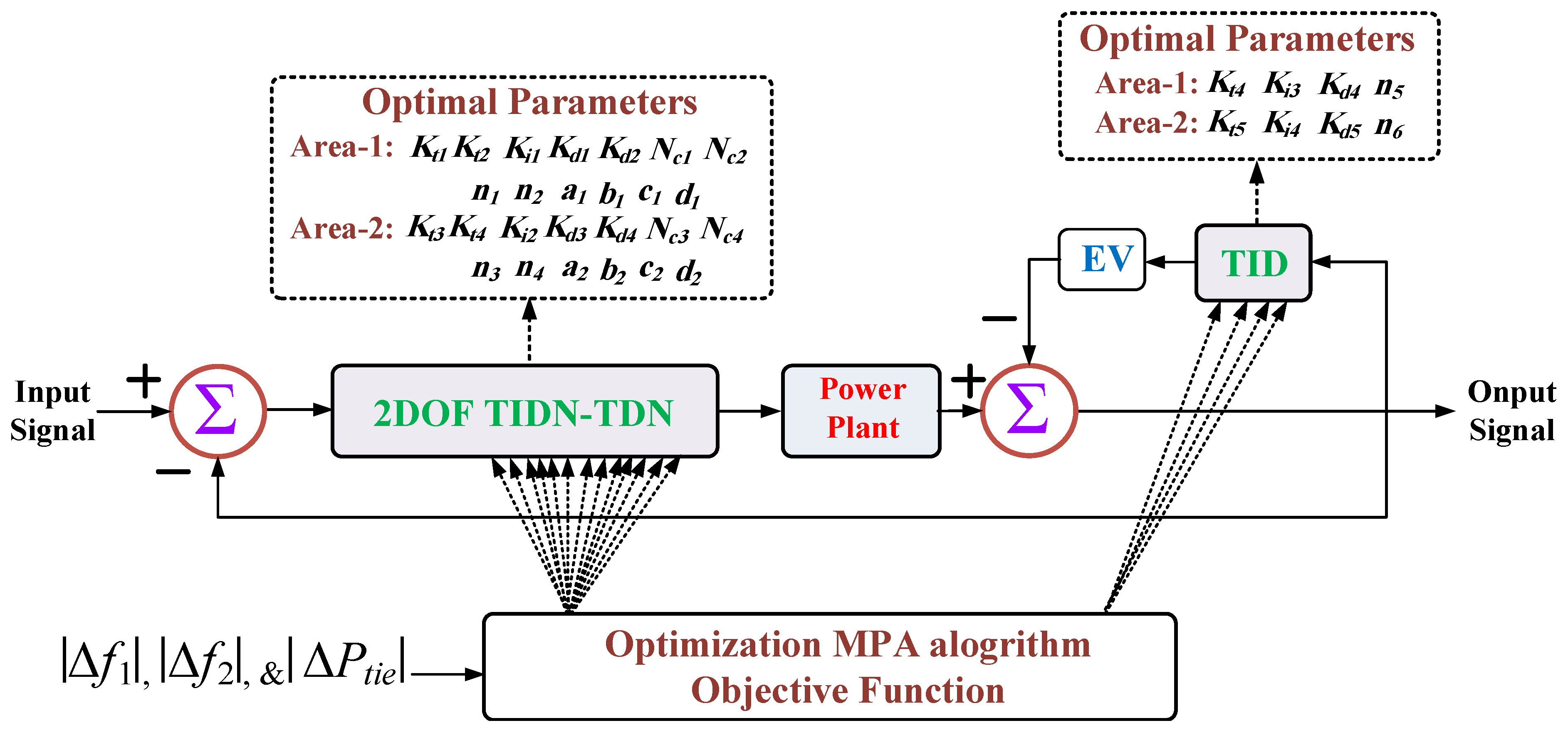
The constraints on the problem are the controller tunable parameters’ boundary limits for both area 1 and area 2. Figure 7 depicts the main diagram representing the MPA-based process for tuning the controllers’ parameters. The design problem can therefore be described as an optimization problem in which the controllers’ parameters can be simultaneously determined based on the minimization of the objective function. The constraint for the TID controller can be represented as [64]
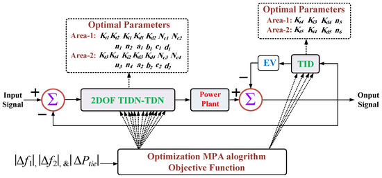
Figure 7.
The optimal parameters of optimized controllers using the MPA algorithm.
However, they are represented for the FOTID controller as follows [45]:
The constraints for the TID-FOPIDN controller are represented as follows [63]:
However, the constraints for the proposed 2DOF TIDN-TDN controller are represented as follows:
where the constraints for various tuned controllers are limited within the maximum limits as and the minimum values of control parameters as . The minimum values of control gains (, , and ) are all zeros, and their maximum (, , and ) values are all five. However, ( and ) are set to 2 and 5, respectively, ( and ) are all zeros, and ( and ) are both set to 1. In addition, ( and ) are set to 5 and 500, respectively. The minimum/maximum tilt/derivative weights (, , , and , , , are between 0 and 4, respectively. The various optimized parameters obtained based on different optimization algorithms such as MPA, PSO, WOA, and GWO are shown in Table 1, Table 2, Table 3 and Table 4, respectively, for the proposed controller, whereas Table 5 summarizes the control parameters of the suggested control methods using the MPA technique.

Table 1.
The coefficient parameters of the proposed controller utilizing the MPA algorithm.
Table 2.
The coefficient parameters of the proposed controller utilizing the PSO algorithm.
Table 3.
The coefficient parameters of the proposed controller utilizing the WOA algorithm.
Table 4.
The coefficient parameters of the proposed controller utilizing the GWO algorithm.
Table 5.
The coefficient parameters of the different controllers utilizing the MPA algorithm.
5.2. The Principle of the MPA Optimizer
As clarified in the literature review, the MPA optimizer has been preferred in several optimum parameter determination applications [61]. The MPA principles are based on food search strategies using Levy and the Brownie movement within their surrounding predators. They determine the optimum by modifying the policy using the biological interaction between prey and predators. In [55], more details about the principles with more details about mathematical representations are given. Based on the literature review, the MPA optimizer has proven superior, with several benefits, as follows:
- High efficiency: The MPA optimizer achieved efficient performance when solving different optimization problems with various properties, particularly where traditional metaheuristic methods fail to converge to optimal solutions.
- Increased robustness: The optimized MPA showed robust performance against changes within optimization problems and has the ability to adapt itself to the different considered types of problem constraints and/or objectives.
- More flexibility: The MPA represents a flexible algorithm, which can be modified and/or customized easily to suit the different optimization problems.
- Scalability: The MPA algorithm was verified and tested on a large variety of optimization problems, wherein it demonstrated promising performance results.
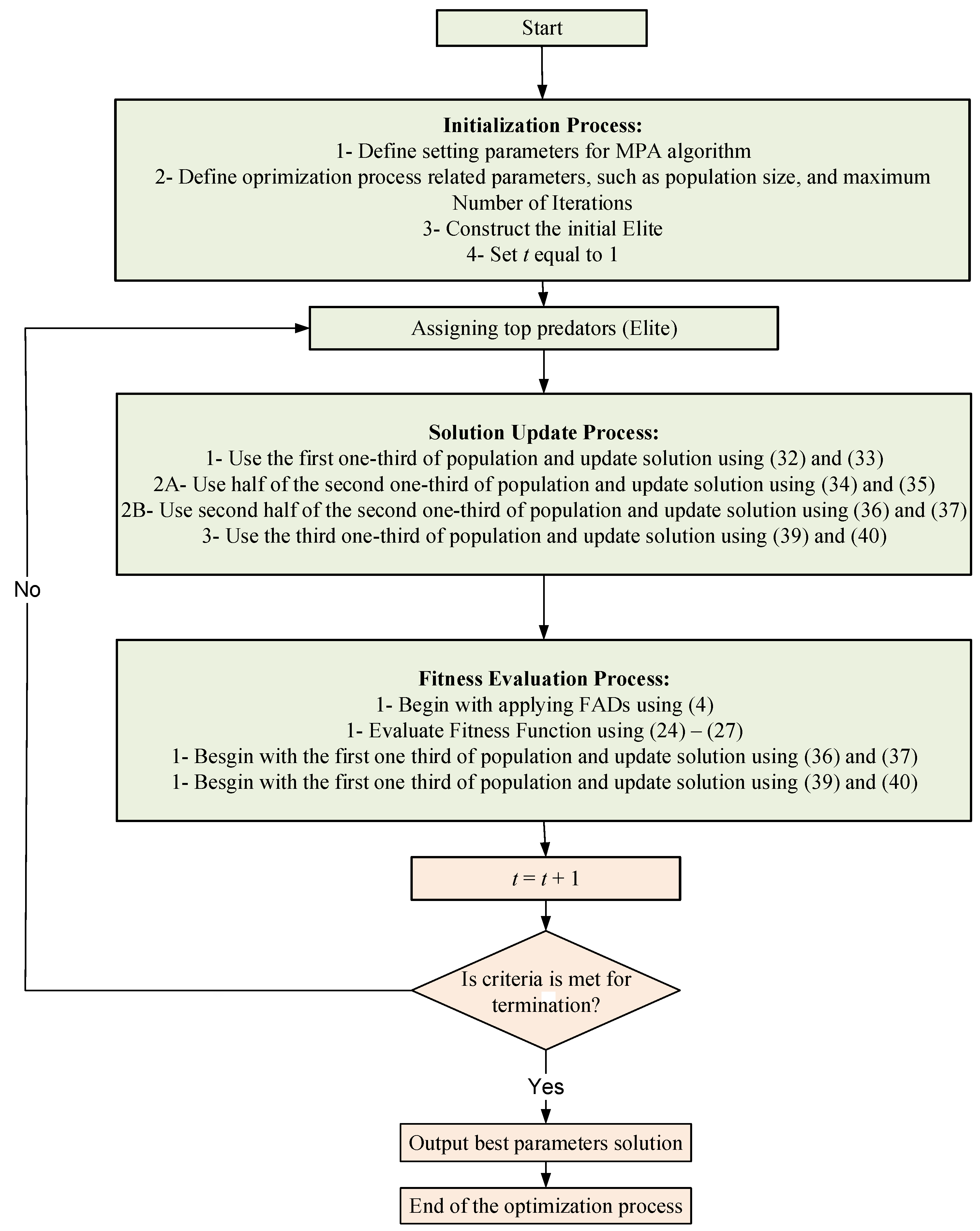
A brief representation of the code and stages is presented in this section. The MPA optimizer has three phases based on the relative speed of the prey and predators. The main stages are shown in the flowchart of the MPA optimizer, shown in Figure 8. Its inherent phases are three phases according to the speed ratio between the prey and predators’ speeds. The stages are as follows:
- High Speed Ratio Phase: It corresponds to the first one-third portion of the iteration number. It is related to cases of higher prey speed than predators. The mathematical representation is given as [55]:where R represents the vector from random numbers within the range, whereas P equals 0.5, and is the Brownian motion vector.
- Unity Speed Ratio Phase: This phase is represented by the second one-third portion of the iterations. It is related to the case of equal speed between prey and predators, in which, the predators’ movements are represented by Brownian expression and the prey’s movements are represented by the Lévy flights model method. Within this phase, the population is divided into two subdivisions. In the first part, (34) and (35) are used, whereas in second part, (36) and (37) are employed for modifying the locations as follows [57]:where is a random variable, and it is generated using Lévy distribution.wherewhere t and are the current value and the maximum value for iterations.
- Low Speed Ratio: This phase is formed by the last one-third of the iteration. In this phase, the prey’s speed is lower than the predators’ speed, in which the location modifications are expressed as follows [55]:In [55], the formation of eddy and fish aggregation devices (FADs) effecting is utilized to count for the surrounding environment conditions of prey and predators. The positions of the population are modified based on FADs to avoid the local optimum solution. It is represented as follows:where is set at 0.2, W is a binary number between 0 and 1, and r stands for a random number. However, and are random indices of prey. and are the lower and upper bounding vectors.
The tuning process is made offline, and thanks to recently developed powerful computers, the control parameters design process has become possible without consuming more time. Moreover, recent advanced digital signal processors facilitated the fractional-order control implementation and application.
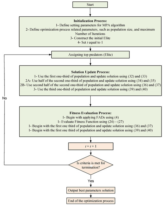
Figure 8.
Flowchart of MPA’s inherent stages and operation.
Figure 8.
Flowchart of MPA’s inherent stages and operation.
6. Simulation Results
In order to improve the LFC of the dual-area MG power systems, this section focuses on the validity and effectiveness of the suggested control technique of the new cascaded 2DOF TIDN-TDN controller coordinated with the EV system. The MPA optimizes the specified control strategy as well as other strategies. The proposed method is checked using the MATLAB/Simulink software 2021a by integrating the two-area system’s Simulink with the algorithm code for the MPA to achieve the LFC fitness function. Using a desktop computer with a processor Intel Core i5 CPU clocked at 2.8 GHz, 64-bit version, the entire code of the dual-area microgrid network is implemented. Utilizing the same technique with the EV model based on the MPA method and under the same operating provisions of load change and RESs disturbances of the thoughtful multiarea MG power network, which implicate a decentralized 2DOF TIDN-TDN controller for the AGC and TID for the EV system in each area, the proposed 2DOF TIDN-TDN concept is established by comparing its interpretation with classical and sophisticated control techniques, such as TID, FOTID, and TID-FOPIDN, and the following operational circumstances for the researched multiarea MG system are investigated in terms of the results:
- Scenario 1: Action of step load perturbation’s effect (SLP).
- Scenario 2: Sudden load shedding (SLS).
- Scenario 3: Parameters uncertainties of nuclear generation.
- Scenario 4: Multiple-load perturbation effects (MLP).
- Scenario 5: The action of high RES deployment.
- Scenario 6: The effect of low inertia 50% (high RES penetration) with multiple-load perturbation and parameter variations in the nuclear power station.
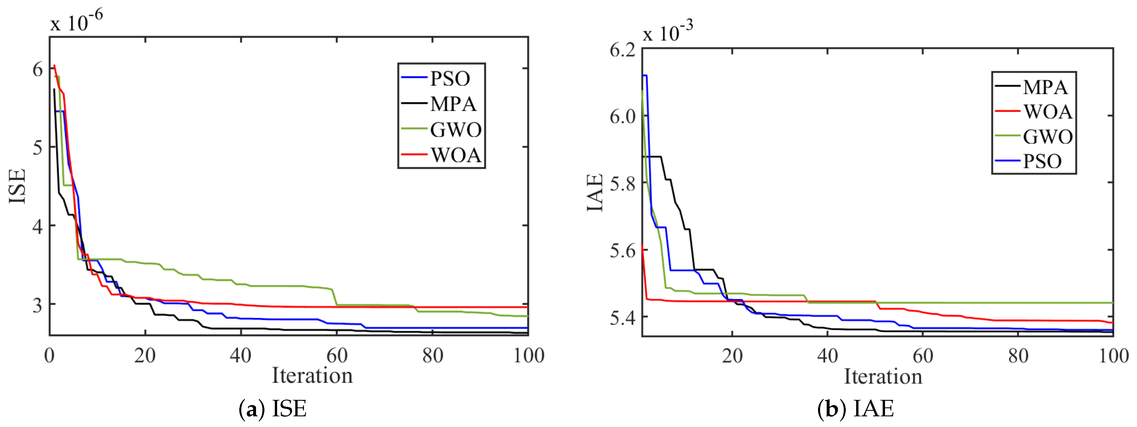
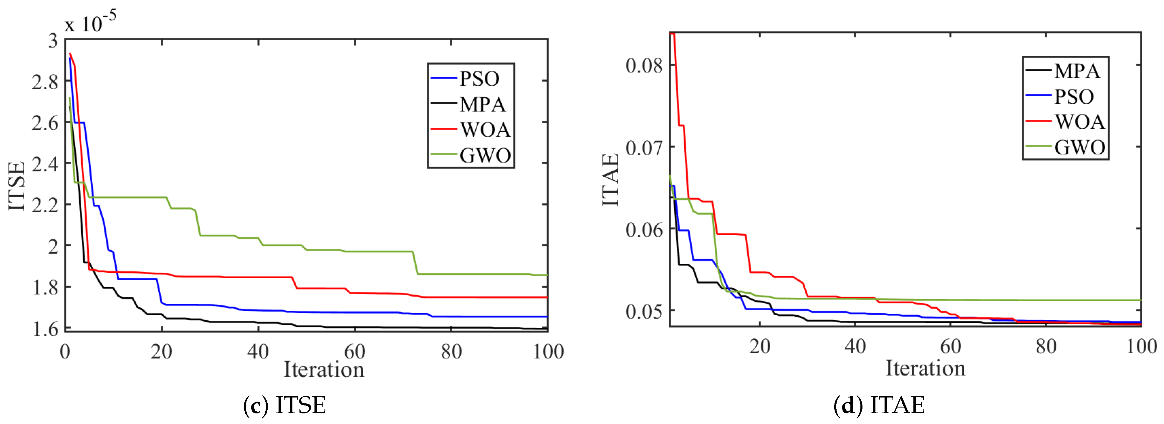
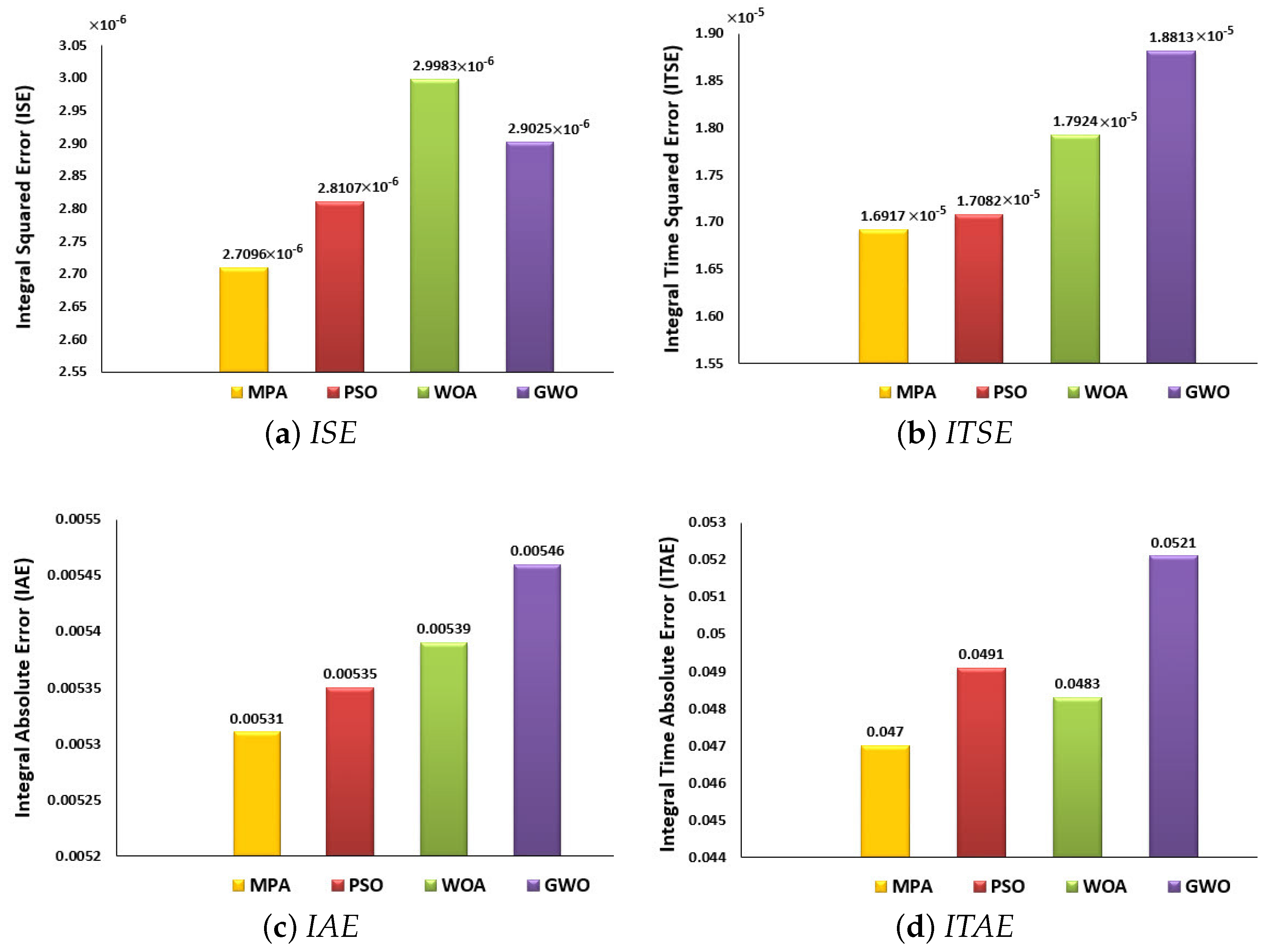
To judge the efficiency of the proposed MPA-based design, its convergence characteristics are compared with the PSO, GWO, and WOA optimizers. The results are obtained using a computer with a Core-i5 CPU 2.8 GHz and a 64-bit system. The results for IAE, ISE, ITSE, and ITAE are shown in Figure 9. In addition, the calculations of the ISE, ITSE, IAE, and ITAE for the studied optimizers are summarized in Table 6. The results show that the lowest objective function minimization is obtained using the MPA method in the case of ISE and ITAE. The PSO comes in second place in these two objectives. Additionally, MPA and PSO share the best convergence characteristics in the IAE and ITSE cases. However, MPA possesses faster convergence to the optimum values compared with that of the PSO method in those two cases.
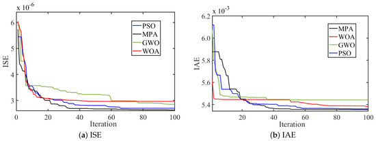
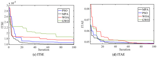
Figure 9.
Convergence characteristics of MPA compared to other optimization techniques.
Table 6.
Comparative analysis of objective function indices for the study of the different PSO, WOA, and GWO algorithms.
6.1. Scenario 1
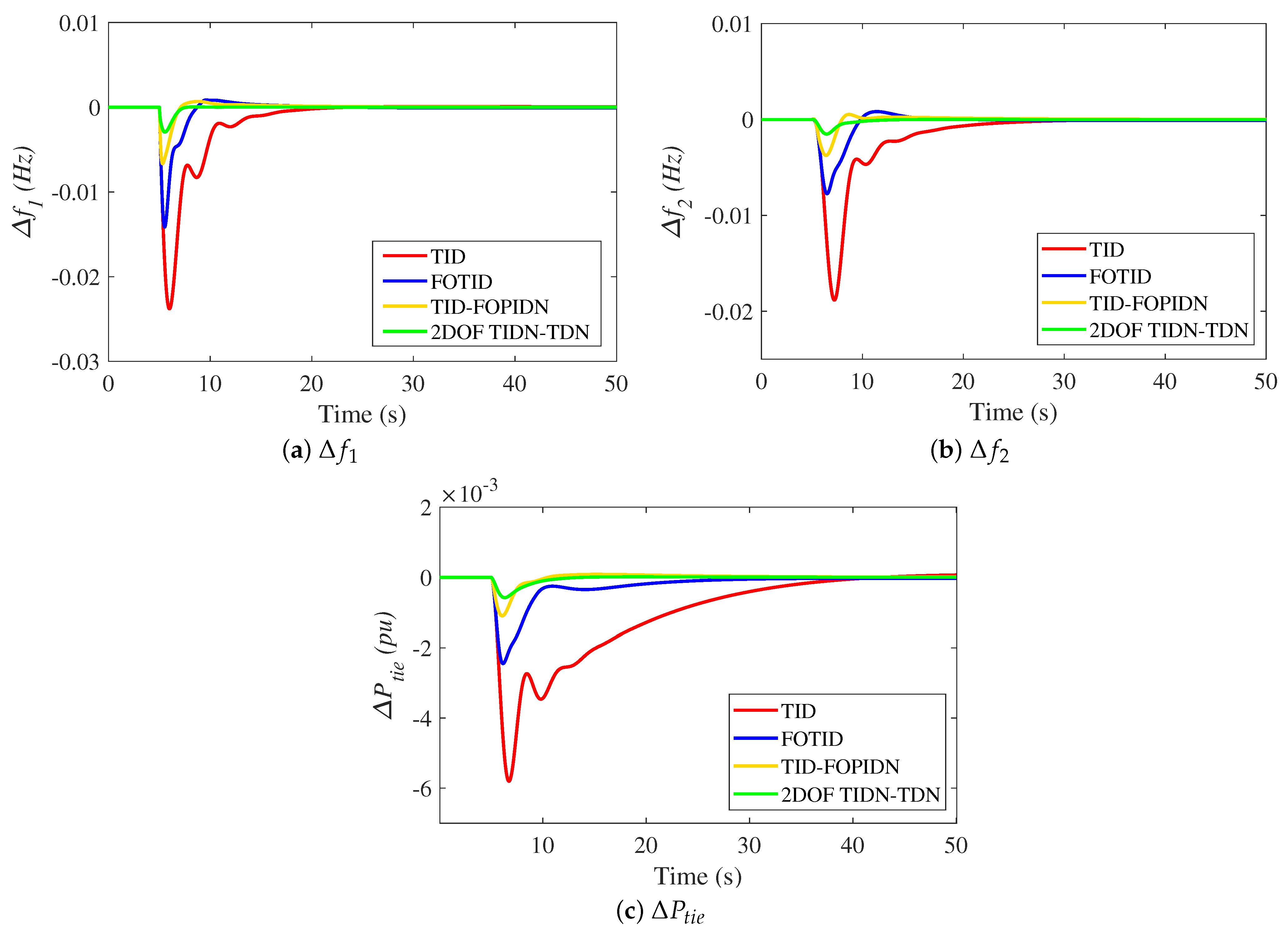
A 20 MW load is installed in area 1 at an instant of 5 s in this scenario for testing the proposed 2DOF TIDN-TDN controller for LFC and TID controller for an EV system on the studied dual-area MG network based on the MPA method, which is verified by comparing it with PSO, WOA, and GWO in this scenario, as noted in Figure 10. As shown in Figure 11, the suggested approach with SLP is compared with TID, FOTID, and TID-FOPIDN controllers for the suggested dual-area network frequency and power diffraction response. The conventional TID controller has the lowest performance in this graph compared with other approaches, with substantial undershoot values at −0.024 Hz in the first area, −0.019 Hz in the second area, and −0.006 p.u. for tie power. FOTID maintained the frequency variation at −0.014 Hz in area 1 and 0.008 Hz in area 2, with −0.0024 p.u in substitution power between the two areas. However, the cascaded TID-FOPIDN controller provided satisfactory results compared with earlier control methods by dampening the system perversions to acceptable levels, as summarized in Table 7. In contrast to other comparable cascaded controllers, the proposed 2DOF TIDN-TDN controller has the fastest response and the lowest oscillations in regulating frequency and power variations. Further comparisons between the suggested controllers are provided in Table 7. The table displays that the proposed 2DOF TIDN-TDN strategy has the smallest peak overshoots (PO), peak undershoots (PU), and settling time (ST) in terms of frequency errors and exchange tie-line power between the multiarea systems. The obtained results state that the inner loop of the two cascaded TID-FOPIDN and 2DOF TIDN-TDN controllers responded to the varied dynamics originating from the different generation sources in both areas, and the outer loop controller can handle the power system dynamics and the SLPs. Therefore, the performance of the proposed cascaded controllers is more influential than that of the other conventional feedback controllers.

Figure 10.
Objective functions comparison in scenario 1: (a) ISE, (b) ITSE, (c) IAE, (d) ITAE.
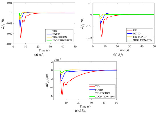
Figure 11.
The frequency response of the dual-MG with step load 1% in scenario 1.
Table 7.
Obtained results for the tested scenarios.
6.2. Scenario 2
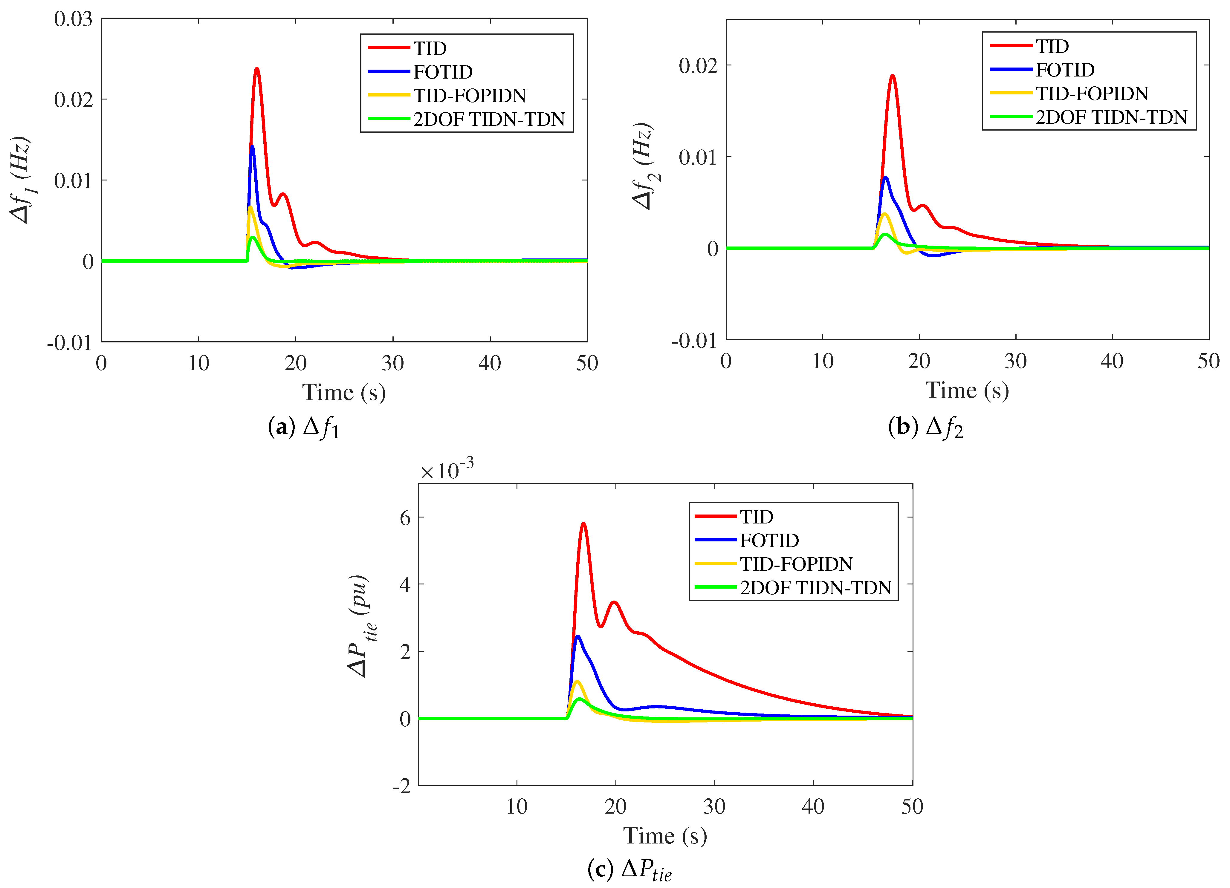
The system frequency and power increase dramatically in the case of sudden load failure, which may disturb the generation/demand balancing condition. Therefore, this scenario tested the performance of all the suggested controllers, in this case, by shedding a 200 MW load in a time of 15 s. Figure 12 shows the impact of this critical situation on the tie-line power change and system frequency deviations. It is distinct that the proposed 2DOF TIDN-TDN controller attains the best performance indices among the other LFCs, since the proposed controller achieves the lowest POs, PUs, and STs. Furthermore, the proposed method can damp the frequency oscillations quickly to their steady-state value after 18 s for the frequency error in area 1, whereas the TID, FOTID, and TID-FOPIDN controllers reach this value after 26 s, 28 s, and 29 s, respectively. Overall, these results ensure the superiority of the multiloop cascaded 2DOF TIDN-TDN and TID-FOPIDN controllers in achieving enhanced and fast responses better than the individual controllers during the critical failure case of microgrid loads.
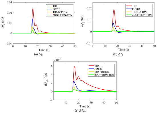
Figure 12.
The frequency response of the dual-MG in scenario 2.
6.3. Scenario 3
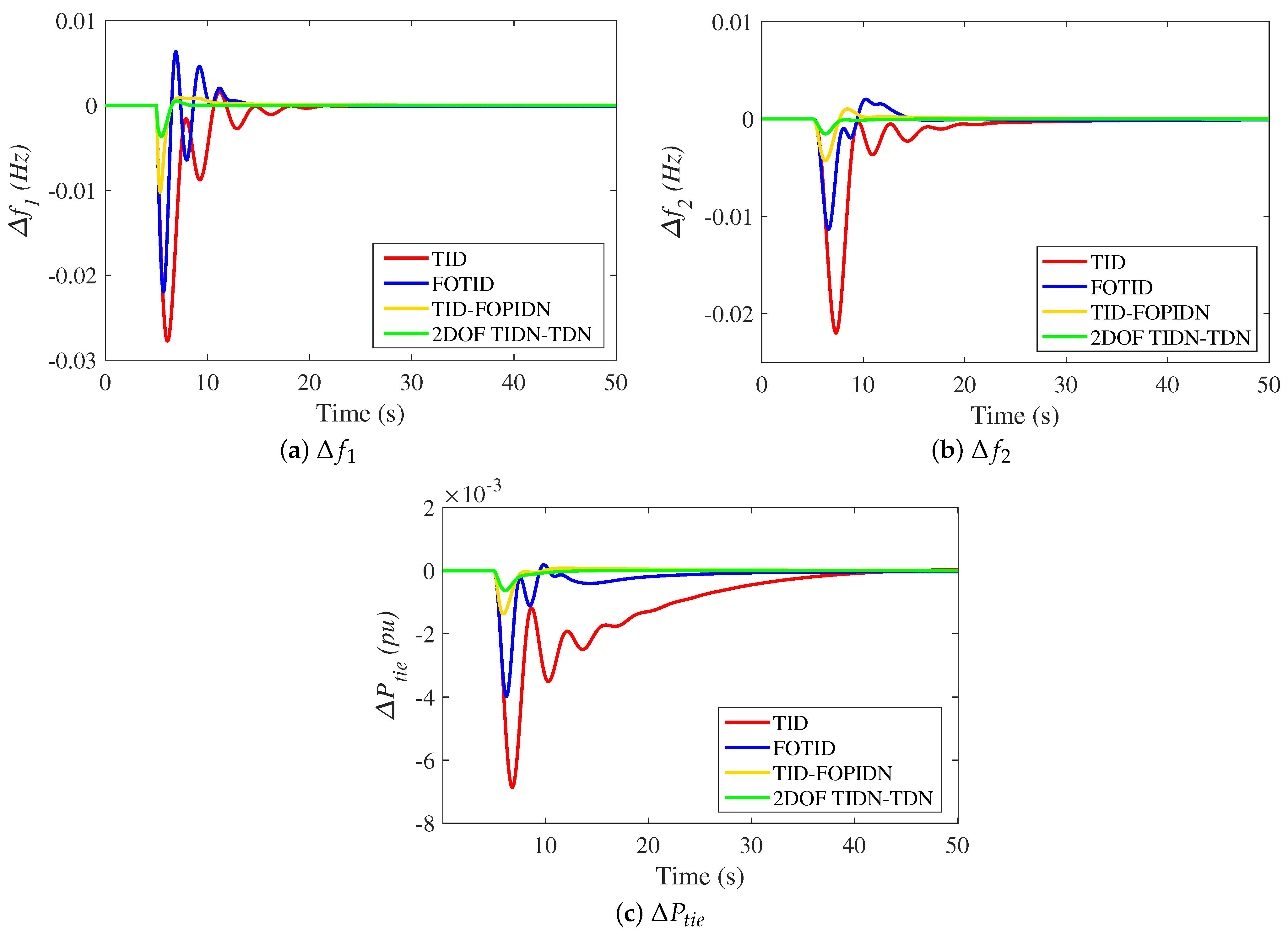
This scenario examined the strength of the proposed coordination-based 2DOF TIDN-TDN as an LFC with EVs using the MPA technique under the impact of parameter uncertainties of the nuclear power plant. However, the parameters of the nuclear plant generation are drastically adjusted in accordance with area 1, [ = +40%, = +70%, = +50%, = +20%, = +30%, = +60%], and area 2, [ = −40%, = −70%, = −50%, = −20%, = −30%, = −60%]. The studied dual-area power network system is tested under the same operating condition as the load perturbation of scenario 1. Figure 13 shows the dynamic responses of , , and of the system, respectively. From the result in this figure, it is evident that when using the TID controller, the frequency deviation is higher compared with previous cases, with undershoot values measuring 0.028 Hz in area 1 and 0.022 Hz in area 2. While the FOTID gave satisfying results with respect to the TID controller, it endured protracted damped oscillations, and it did not have the ability to retrieve the frequency to its steady-state value in a short time duration. However, the cascaded TID-FOPIDN preserved the system frequency at 0.01 Hz in area 1 and at 0.004 Hz in area 2, and the perversion of the power in the tie-line is 0.00494 p.u. On the other hand, the new cascaded 2DOF TIDN-TDN controller is the quickest in curbing the frequency and tie-line power deviations, and it has a lower steady-state error value than that presented by other traditional and cascaded controllers.
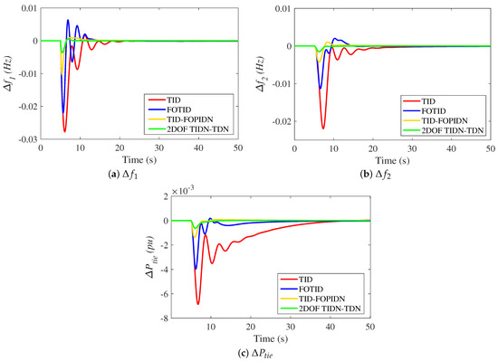
Figure 13.
The dynamic response of the system in scenario 3.
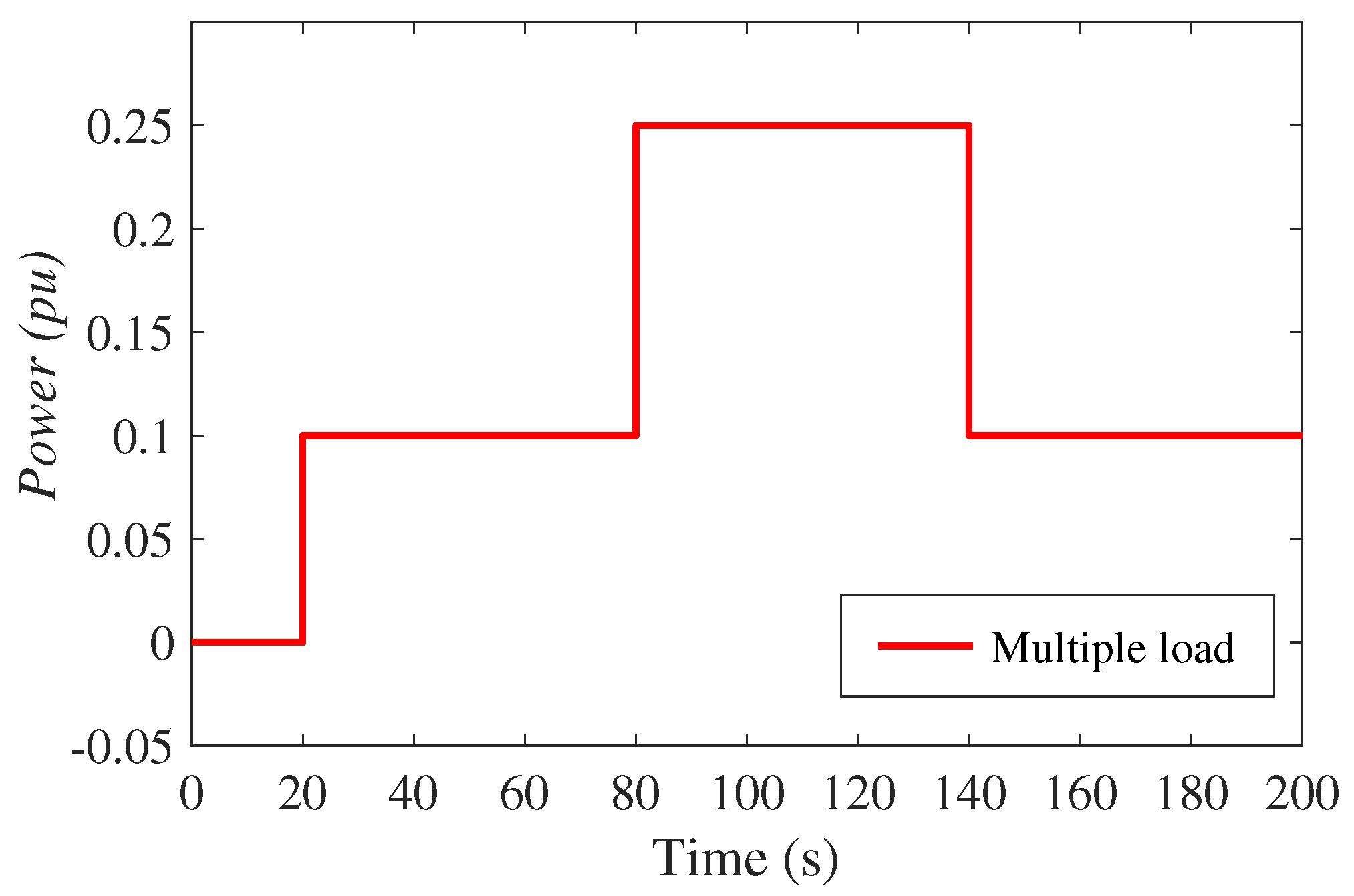
6.4. Scenario 4
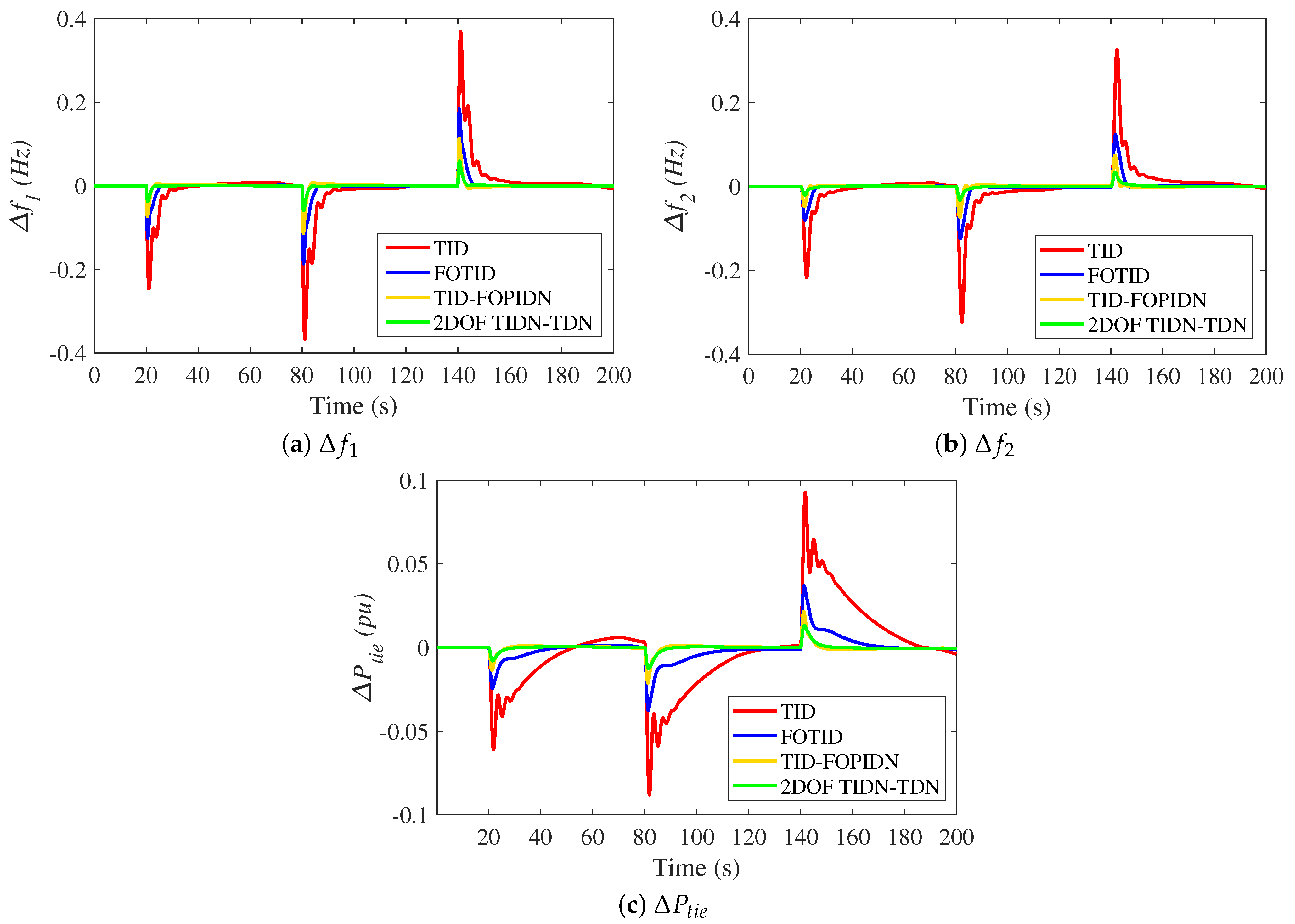
The substantial target of this study case is to elucidate the interpretation of the proposed cascaded 2DOF TIDN-TDN control scheme based on the MPA algorithm under the influence of load parameter uncertainties due to multiple-load demands, as depicted in Figure 14 of this scenario. Figure 15 shows the dynamic frequency and energy exchange of the multi-microgrid system due to this significant load change. It is noticed that the proposed 2DOF TIDN-TDN controller has faster action with the slightest deviations compared with other control techniques, especially at the instant of the worst load shift in this scenario (t = 140 s). It can minimize the frequency diffractions in the first area 85.92%, 74.1%, and 60% better than the TID, FOTID, and TID-FOPIDN controllers, respectively. Additionally, it can demoralize the frequency vibrations in the second area with percentage gains of 91.9%, 80.85%, and 68.42% compared with the TID, FOTID, and TID-FOPIDN controllers, respectively. Furthermore, Table 7 shows that the proposed cascaded 2DOF TIDN-TDN controller has the lowest tie-line exchange power when compared with the other methods. The calculations of ISE, ITSE, IAE, and ITAE for all the studied scenarios are summarized in Table 8. Moreover, it is clear from this discussion that the percentage coordination of the LFC and EV participation utilizing the new 2DOF TIDN-TDN controller based on the efficient MPA technique yields the best results through the three-step load changes in this scenario. This is due to the function of the inner loop 2DOF-TDN of the proposed controller schematic responding quickly to the variation in the load demand. Furthermore, the results manifest that the other single-loop structures have a phase lag regarding the multiple-load disturbances compared with the suggested cascaded controllers.
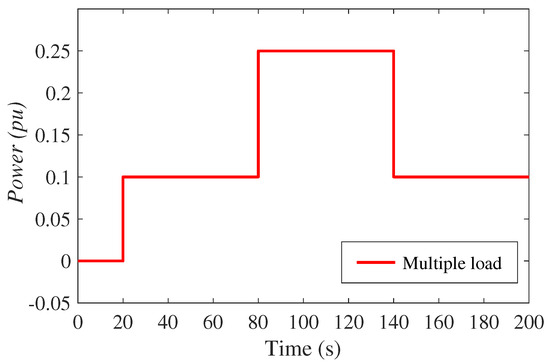
Figure 14.
Generation profiles for Scenario 4.
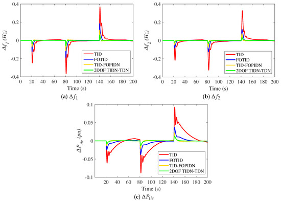
Figure 15.
The frequency response of the dual-MG in scenario 4.
Table 8.
Different objective function indices for suggested controllers.
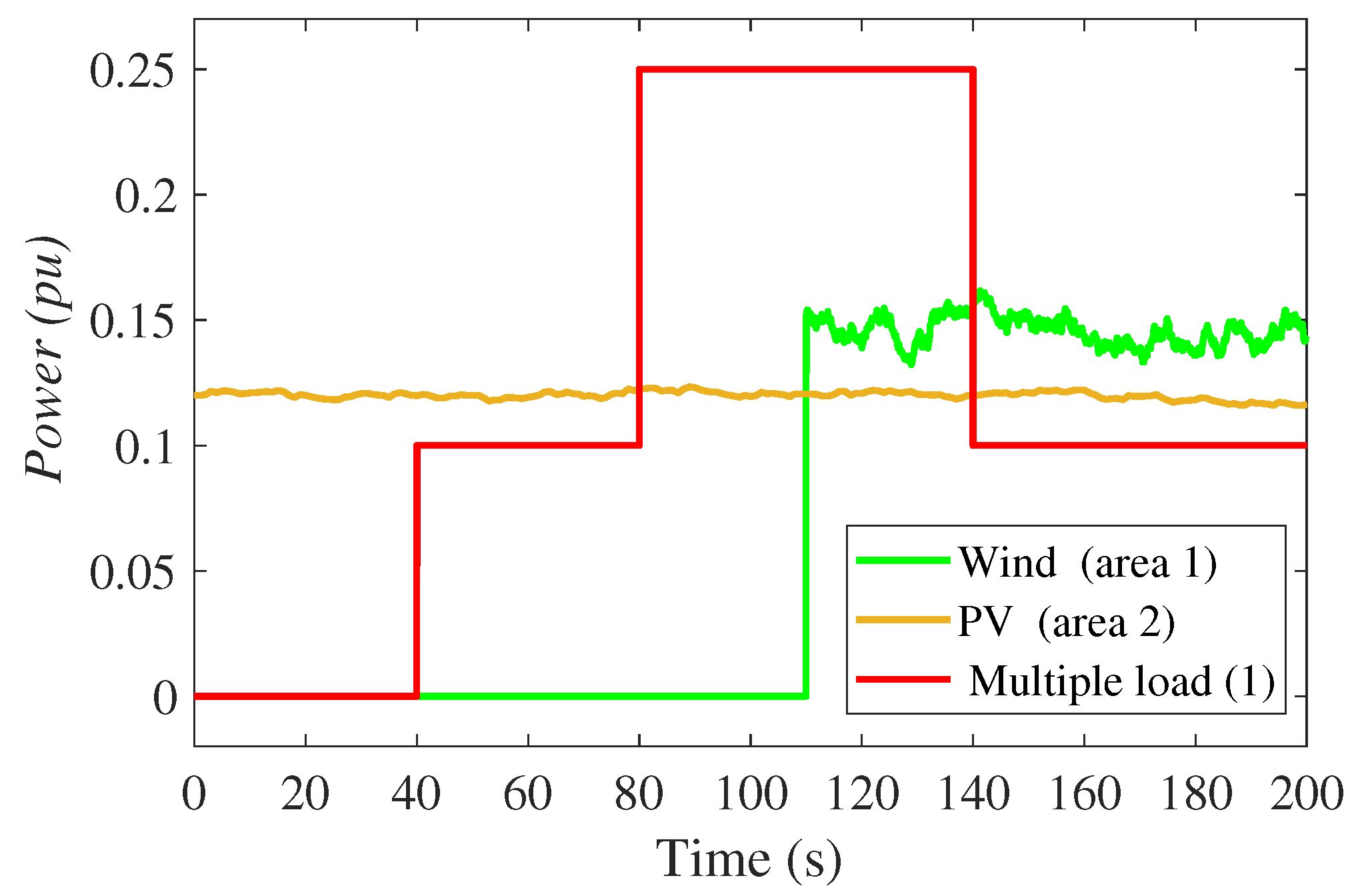
6.5. Scenario 5
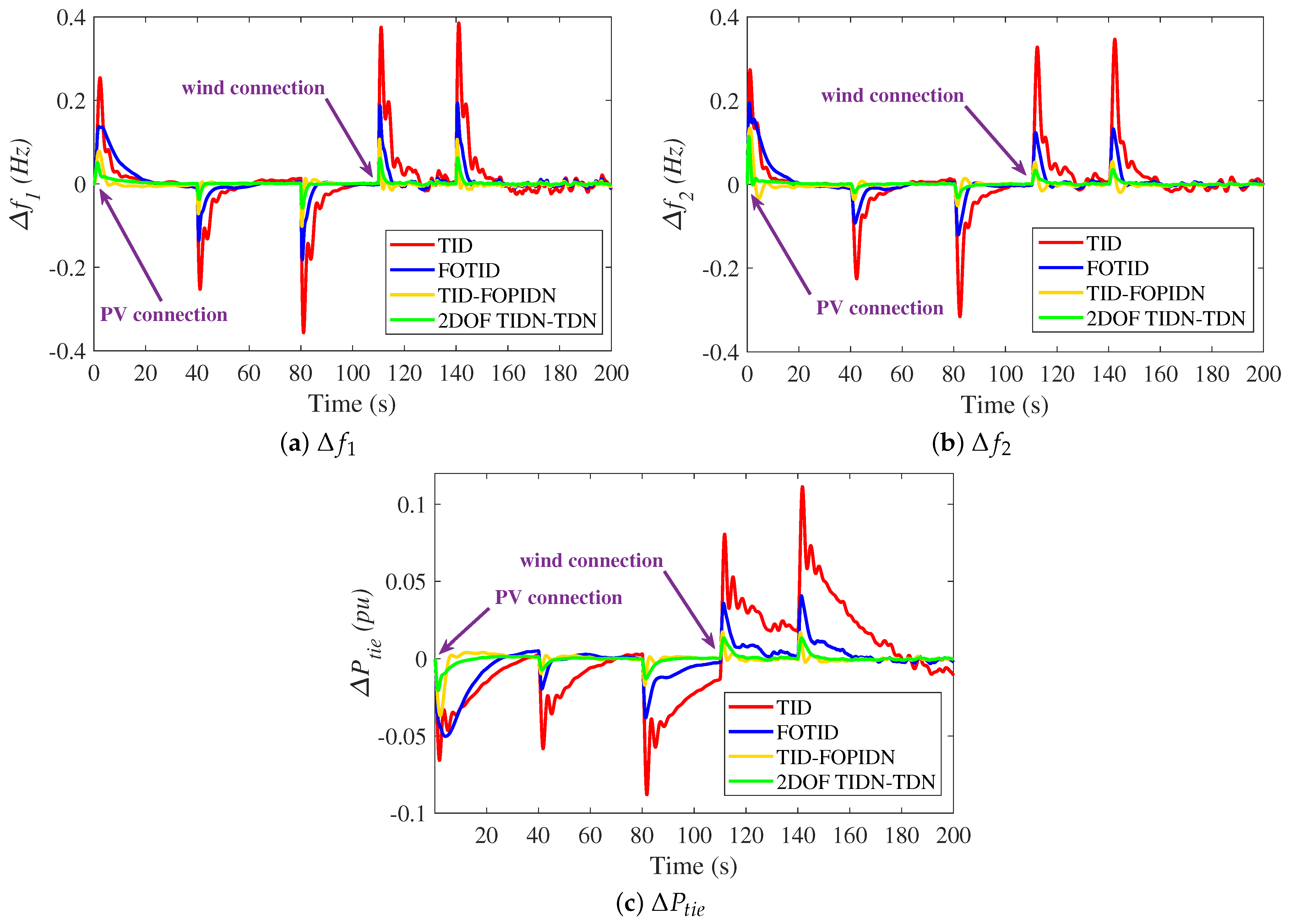
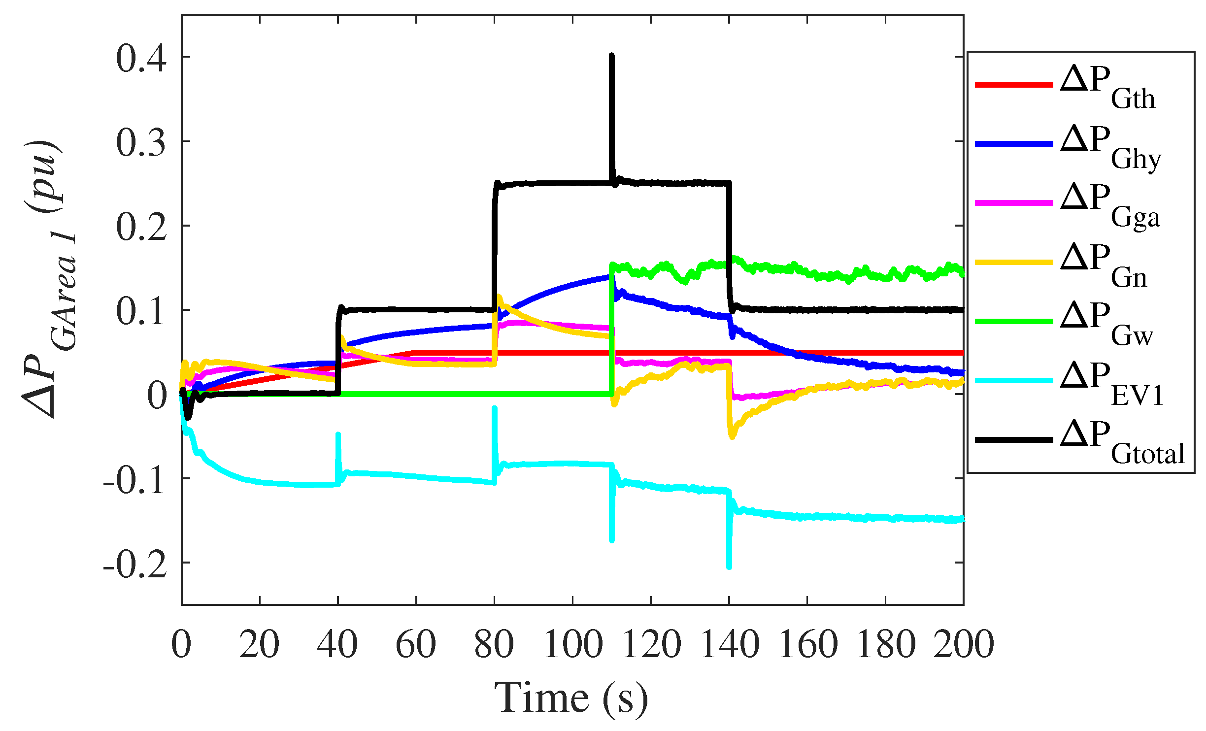
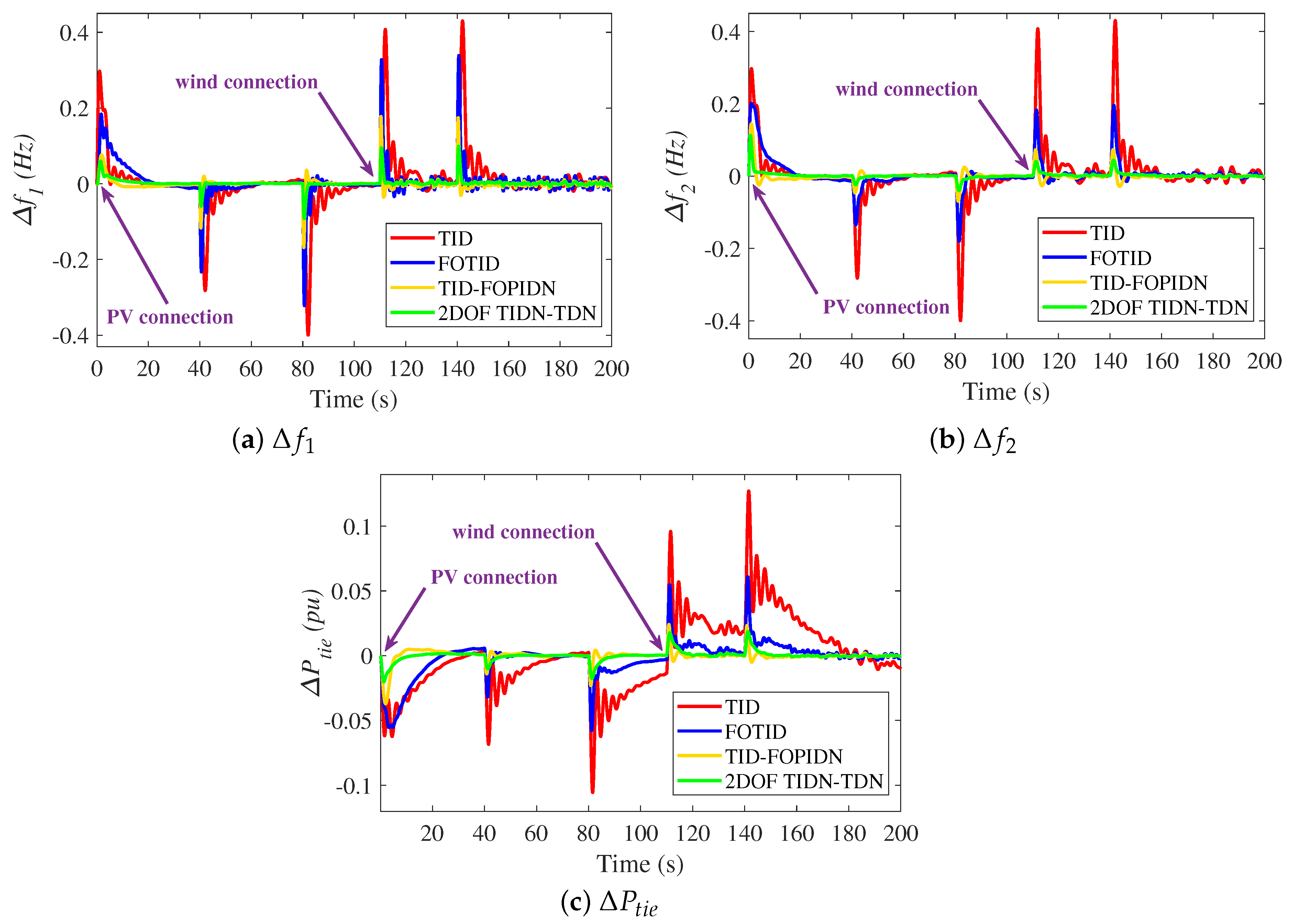
This study tests the novel cascaded 2DOF TIDN-TDN controller, augmented with EV participation in the LFC loop, under severe disturbance conditions involving high levels of RES penetration. However, the PV power unit is connected at the initial time, while the wind power is integrated at 110 s, in addition to the effect of multiple-load changes, as shown in Figure 16. Figure 17 illustrates the obtained comparative results for the frequency and tie-line power in this case. It is clear that the fluctuation of and is close to +0.4 Hz, and more than 0.06 p.u. in tie-line power is achieved by using the TID controller. It is followed by the FOTID controller, with a variation in +0.2 Hz in both power system zones. While the two cascaded TID-FOPIDN and 2DOF TIDN-TDN controllers give deviations around +0.1 Hz and 0.08 Hz in area 1 and area 2, respectively, the proposed 2DOF TIDN-TDN controller is efficient and controls the deviations within the lowest time frame with minimum overshoot and undershoot values, especially at the severe load variations instants at 40 s and 80 s. This, in turn, confirms that the new proposed controller acquires superior performance when compared with the other used controllers. In addition, these results prove that the proposed cascaded 2DOF TIDN-TDN controller has a very fast inner control loop, which can respond more quickly to disturbances of load and RES than its outer loop. From another approach, the cascaded (2DOF TIDN-TDN) control signal, which is applied to the conventional power generators and energy storage devices in both area (a) and (b) enables the EVs to have a fast performance in the charge/discharge process and obtain less power from these generators than the other addressed controllers, as shown in Figure 18 and Figure 19, respectively. Therefore, it is clear from this result’s explanation that the proposed cascaded 2DOF TIDN-TDN controller based on the MPA technique is the most effective one in this scenario.
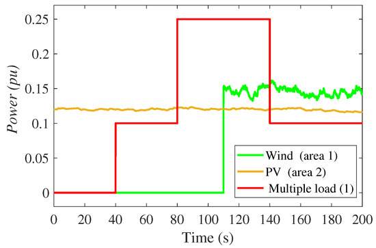
Figure 16.
Profiles of different generators for Scenario 5.
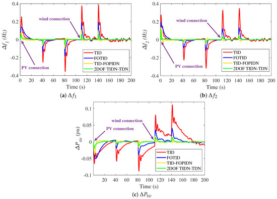
Figure 17.
The frequency response of the dual-MG in scenario 5.
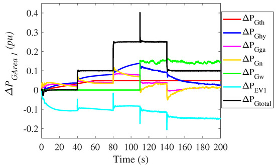
Figure 18.
Power generations of area 1 for scenario 5.
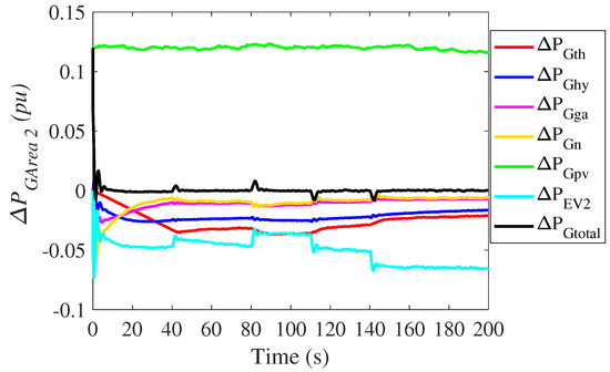
Figure 19.
Power generations of area 2 for scenario 5.
6.6. Scenario 6
To scrutinize the interpretation of the proposed 2DOF TIDN-TDN controller, the system is submitted to high perturbations, such as multistep load perturbation, RES power fluctuations, and parameter changes that could cause system instability. In this case, the MG network parameters were changed as follows: low system inertia (i.e., 50% alleviation of its nominal values in two-area) and changes in the parameters of the nuclear plant generation in accordance with area 1, [ = +40%, = +70%, = +50%, = +20%, = +30%, = +60%], and area 2, [ = −40%, = −70%, = −50%, = −20%, = −30%, = −60%], under the same operating conditions discussed in scenario 4. The obtained results are shown in Figure 20. It is observed that the TID and FOTID controllers have the lowest performance for all perturbation stipulations in this scenario. For instance, the obtained values at 40 s for are 0.28, 0.18, 0.11, and 0.056 for the TIDF, FOTID, TID-FOPIDN, and the 2DOF TIDN-TDN, respectively. It is obvious that the proposed approach acquires the minimum values of the measured PO, PU, and ST in , , and .

Figure 20.
The frequency response of the dual-MG in scenario 6.
6.7. Stability Analysis of the Closed-Loop System
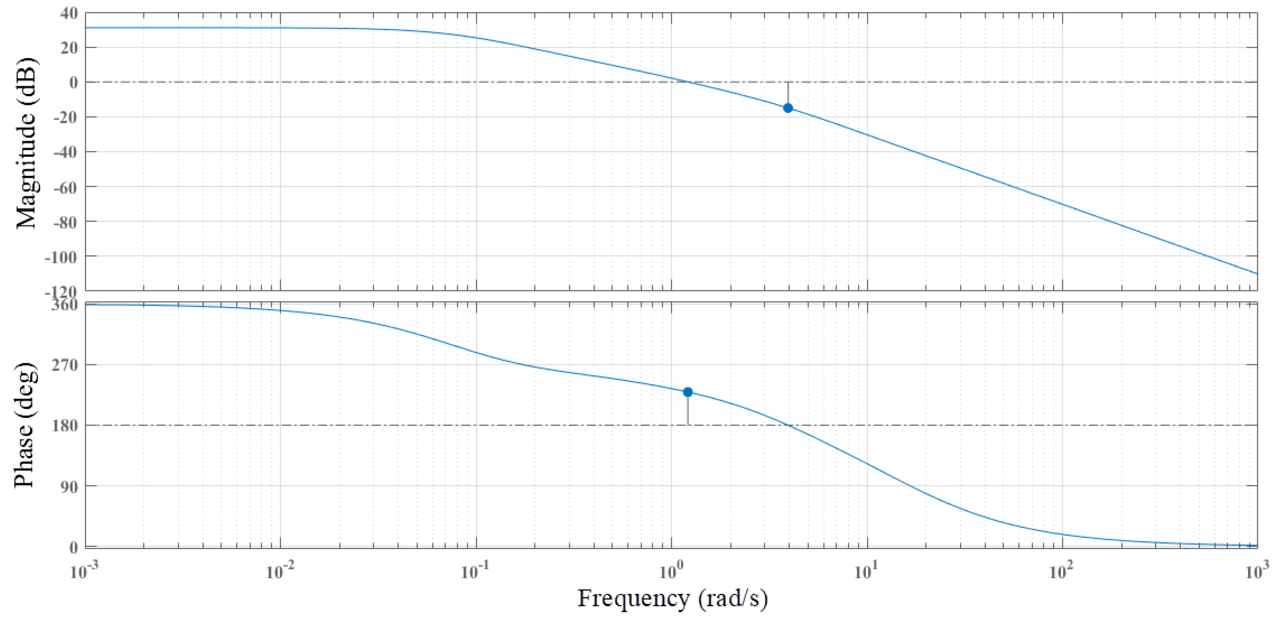
Based on the studied system modeling and the proposed 2DOF (TIDN-TDN) controller, a stability analysis based on the Bode diagram plot is performed. Figure 21 shows the Bode plot of the examined system loop gains with the proposed controller. The magnitude of the gain margin plot is more steady for all frequencies, according to Figure 21. As a result, the phase margin is infinite, displaying that the proposed controller is able to deal with system uncertainty.
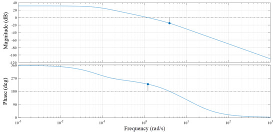
Figure 21.
Bode plot of the examined system loop gains with the proposed controller.
7. Conclusions
An optimized 2DOF TIDN-TDN controller was proposed in this paper for the LFC of multisourced interconnected power systems. The proposed controller uses the frequency signals in the inner loops, which enables the mitigation of high-frequency disturbances. Moreover, it uses the ACE in the outer loop, which results in mitigating the low-frequency disturbances. Additionally, the powerful recent marine predator optimizer algorithm (MPA) is proposed for the simultaneous optimization of the LFC and EV controllers’ parameters in different areas. Therefore, improved optimum performance is achieved using the proposed MPA-based optimized 2DOF TIDN-TDN controller. Moreover, coordination of EV control is proposed to contribute to mitigating existing disturbances in the power systems (vehicle-to-grid V2G concept). The proposed controller and optimized design were tested and compared using the RES highly penetrated dual-area power systems. The acquired results confirm the superior performance measurements of the proposed 2DOF TIDN-TDN controller over the existing TID, FOTID, cascaded TID-FOPIDN controller. For instance, at step load change, the maximum undershoot in the first area frequency is 0.003 p.u. using the proposed controller compared with 0.007, 0.015, and 0.024 with TID-FOPIDN, FOTID, and TID, respectively. The estimated ISEs in this case were 2.7096 , 1.1264 , 5.9414 , and 4.0164 using the proposed 2DOF TIDN-TDN, TID-FOPIDN, FOTID, and TID, respectively. This signifies that the proposed 2DOF TIDN-TDN LFC has ISE values of 24.06%, 4.56%, and 0.67% compared with TID-FOPIDN, FOTID, and TID, respectively. Future work includes frequency-domain stability analysis and comparison of the fractional-order cascaded controllers. In addition, the consideration of existing communication delays can be presented and investigated from the control design and stability analysis side.
Author Contributions
Conceptualization, A.S., M.A. and E.A.M.; Methodology, A.H.; Software, B.A., M.A., A.E., M.K. and E.A.M.; Validation, A.H., M.A.A. and A.E.; Formal analysis, M.A., M.K. and E.A.M.; Investigation, M.M.A., M.A.A. and A.S.; Resources, A.S. and M.A.; Data curation, M.M.A. and A.E.; Writing—original draft, A.H.; Writing—review & editing, M.A. and E.A.M.; Visualization, B.A.; Supervision, M.M.A. All authors have read and agreed to the published version of the manuscript.
Funding
The authors extend their appreciation to the Deputyship for Research & Innovation, Ministry of Education in Saudi Arabia for funding this research work through the project number (445-9-510).
Data Availability Statement
No new data were created or analyzed in this study. Data sharing is not applicable to this article.
Conflicts of Interest
The authors declare no conflict of interest.
Appendix A
System’s basic parameters [63,64,65,68]:
LFC: ,, = 2.4 Hz/MW. , = 0.4312 MW/Hz. Power system: , = 68.9655, , = 11.49 s, = 0.0433, = −1. Thermal plant = 846 MW: = 0.08 s, = 0.3 s, = 0.3, = 10 s, = 0.486207. Hydro plant = 467 MW: = 0.2 s, = 28.749 s, = 5 s, = 1 s, = 0.268391. Gas plant = 227 MW: = 0.049 s, = 1, = 0.6 s, = 1.1 s, = 0.01 s, = 0.239 s, = 0.2 s, = 0.130459. Nuclear plant = 200 MW: = 2, = 0.5 s, = 0.3, = 7 s, = 9 s, = 0.08 s, = 0.114943. PV plant: = 1.3 s, = 1. Wind plant: = 1.5 s, = 1. EV: Penetration Level = 5–10%, = 364.8 V, = 66.2 Ah, = 0.074 ohms, = 0.047 ohms, = 703.6 farad, = 0.02612, Maximum = 95%, = 24.15 kWh.
References
- Ali, M.; Kotb, H.; AboRas, M.K.; Abbasy, H.N. Frequency regulation of hybrid multi-area power system using wild horse optimizer based new combined Fuzzy Fractional-Order PI and TID controllers. Alex. Eng. J. 2022, 61, 12187–12210. [Google Scholar] [CrossRef]
- Ramshanker, A.; Chakraborty, S.; Elangovan, D.; Kotb, H.; Aboras, K.M.; Giri, N.C.; Agyekum, E.B. CO2 Emission Analysis for Different Types of Electric Vehicles When Charged from Floating Solar Photovoltaic Systems. Appl. Sci. 2022, 12, 12552. [Google Scholar] [CrossRef]
- Li, S.; Shao, X.; Zhang, W.; Zhang, Q. Distributed Multicircular Circumnavigation Control for UAVs with Desired Angular Spacing. Def. Technol. 2023. [Google Scholar] [CrossRef]
- Zhang, F.; Shao, X.; Xia, Y.; Zhang, W. Elliptical encirclement control capable of reinforcing performances for UAVs around a dynamic target. Def. Technol. 2023. [Google Scholar] [CrossRef]
- Zhang, J.; Shao, X.; Zhang, W.; Na, J. Path-Following Control Capable of Reinforcing Transient Performances for Networked Mobile Robots Over a Single Curve. IEEE Trans. Instrum. Meas. 2023, 72, 1–12. [Google Scholar] [CrossRef]
- Shao, X.; Li, S.; Zhang, J.; Zhang, F.; Zhang, W.; Zhang, Q. GPS-free Collaborative Elliptical Circumnavigation Control for Multiple Non-holonomic Vehicles. IEEE Trans. Intell. Veh. 2023, 8, 3750–3761. [Google Scholar] [CrossRef]
- Zhang, J.; Shao, X.; Zhang, W.; Zuo, Z. Multi-circular formation control with reinforced transient profiles for nonholonomic vehicles: A path-following framework. Def. Technol. 2023. [Google Scholar] [CrossRef]
- Bakhtadze, N.; Maximov, E.; Maximova, N. Digital Identification Algorithms for Primary Frequency Control in Unified Power System. Mathematics 2021, 9, 2875. [Google Scholar] [CrossRef]
- Ranjan, M.; Shankar, R. A literature survey on load frequency control considering renewable energy integration in power system: Recent trends and future prospects. J. Energy Storage 2022, 45, 103717. [Google Scholar] [CrossRef]
- Dreidy, M.; Mokhlis, H.; Mekhilef, S. Inertia response and frequency control techniques for renewable energy sources: A review. Renew. Sustain. Energy Rev. 2017, 69, 144–155. [Google Scholar] [CrossRef]
- Shankar, R.; Pradhan, S.; Chatterjee, K.; Mandal, R. A comprehensive state of the art literature survey on LFC mechanism for power system. Renew. Sustain. Energy Rev. 2017, 76, 1185–1207. [Google Scholar] [CrossRef]
- Khamies, M.; Magdy, G.; Ebeed, M.; Kamel, S. A robust PID controller based on linear quadratic gaussian approach for improving frequency stability of power systems considering renewables. ISA Trans. 2021, 117, 118–138. [Google Scholar] [CrossRef] [PubMed]
- Fernández-Guillamón, A.; Gómez-Lázaro, E.; Muljadi, E.; Molina-García, Á. Power systems with high renewable energy sources: A review of inertia and frequency control strategies over time. Renew. Sustain. Energy Rev. 2019, 115, 109369. [Google Scholar] [CrossRef]
- Pandey, S.K.; Mohanty, S.R.; Kishor, N. A literature survey on load–frequency control for conventional and distribution generation power systems. Renew. Sustain. Energy Rev. 2013, 25, 318–334. [Google Scholar] [CrossRef]
- Lv, X.; Sun, Y.; Wang, Y.; Dinavahi, V. Adaptive Event-Triggered Load Frequency Control of Multi-Area Power Systems Under Networked Environment via Sliding Mode Control. IEEE Access 2020, 8, 86585–86594. [Google Scholar] [CrossRef]
- Kavikumar, R.; Kwon, O.M.; Lee, S.H.; Sakthivel, R. Input-output finite-time IT2 fuzzy dynamic sliding mode control for fractional-order nonlinear systems. Nonlinear Dyn. 2022, 108, 3745–3760. [Google Scholar] [CrossRef]
- Sakthivel, R.; Kavikumar, R.; Ma, Y.K.; Ren, Y.; Marshal Anthoni, S. Observer-Based H∞ Repetitive Control for Fractional-Order Interval Type-2 TS Fuzzy Systems. IEEE Access 2018, 6, 49828–49837. [Google Scholar] [CrossRef]
- Vrdoljak, K.; Perić, N.; Petrović, I. Sliding mode based load-frequency control in power systems. Electr. Power Syst. Res. 2010, 80, 514–527. [Google Scholar] [CrossRef]
- Pan, C.; Liaw, C. An adaptive controller for power system load-frequency control. IEEE Trans. Power Syst. 1989, 4, 122–128. [Google Scholar] [CrossRef]
- Rakhshani, E.; Rodriguez, P.; Cantarellas, A.M.; Remon, D. Analysis of derivative control based virtual inertia in multi-area high-voltage direct current interconnected power systems. IET Gener. Transm. Distrib. 2016, 10, 1458–1469. [Google Scholar] [CrossRef]
- Kerdphol, T.; Rahman, F.S.; Mitani, Y.; Watanabe, M.; Kufeoglu, S. Robust Virtual Inertia Control of an Islanded Microgrid Considering High Penetration of Renewable Energy. IEEE Access 2018, 6, 625–636. [Google Scholar] [CrossRef]
- Kocaarslan, I.; Çam, E. Fuzzy logic controller in interconnected electrical power systems for load-frequency control. Int. J. Electr. Power Energy Syst. 2005, 27, 542–549. [Google Scholar] [CrossRef]
- Bu, X.; Yu, W.; Cui, L.; Hou, Z.; Chen, Z. Event-Triggered Data-Driven Load Frequency Control for Multiarea Power Systems. IEEE Trans. Ind. Inform. 2022, 18, 5982–5991. [Google Scholar] [CrossRef]
- Latif, A.; Hussain, S.S.; Das, D.C.; Ustun, T.S.; Iqbal, A. A review on fractional order (FO) controllers’ optimization for load frequency stabilization in power networks. Energy Rep. 2021, 7, 4009–4021. [Google Scholar] [CrossRef]
- Morgan, E.F.; El-Sehiemy, R.A.; Awopone, A.K.; Megahed, T.F.; Abdelkader, S.M. Load Frequency Control of Interconnected Power System Using Artificial Hummingbird Optimization. In Proceedings of the 2022 23rd International Middle East Power Systems Conference (MEPCON), Cairo, Egypt, 13–15 December 2022. [Google Scholar] [CrossRef]
- Elmelegi, A.; Mohamed, E.A.; Aly, M.; Ahmed, E.M. An Enhanced Slime Mould Algorithm Optimized LFC Scheme for Interconnected Power Systems. In Proceedings of the 2021 22nd International Middle East Power Systems Conference (MEPCON), Assiut, Egypt, 14–16 December 2021. [Google Scholar] [CrossRef]
- Khokhar, B.; Dahiya, S.; Singh Parmar, K.P. Atom search optimization based study of frequency deviation response of a hybrid power system. In Proceedings of the 2020 IEEE 9th Power India International Conference (PIICON), Sonepat, India, 28 February–1 March 2020; pp. 1–5. [Google Scholar] [CrossRef]
- Panda, S.; Mohanty, B.; Hota, P. Hybrid BFOA-PSO algorithm for automatic generation control of linear and nonlinear interconnected power systems. Appl. Soft Comput. 2013, 13, 4718–4730. [Google Scholar] [CrossRef]
- Arora, K.; Kumar, A.; Kamboj, V.K.; Prashar, D.; Shrestha, B.; Joshi, G.P. Impact of Renewable Energy Sources into Multi Area Multi-Source Load Frequency Control of Interrelated Power System. Mathematics 2021, 9, 186. [Google Scholar] [CrossRef]
- Gupta, D.K.; Soni, A.K.; Jha, A.V.; Mishra, S.K.; Appasani, B.; Srinivasulu, A.; Bizon, N.; Thounthong, P. Hybrid Gravitational–Firefly Algorithm-Based Load Frequency Control for Hydrothermal Two-Area System. Mathematics 2021, 9, 712. [Google Scholar] [CrossRef]
- Yousri, D.; Babu, T.S.; Fathy, A. Recent methodology based Harris Hawks optimizer for designing load frequency control incorporated in multi-interconnected renewable energy plants. Sustain. Energy Grids Netw. 2020, 22, 100352. [Google Scholar] [CrossRef]
- Salama, H.S.; Magdy, G.; Bakeer, A.; Vokony, I. Adaptive coordination control strategy of renewable energy sources, hydrogen production unit, and fuel cell for frequency regulation of a hybrid distributed power system. Prot. Control. Mod. Power Syst. 2022, 7, 34. [Google Scholar] [CrossRef]
- Kumar, A.; Gupta, D.K.; Ghatak, S.R.; Appasani, B.; Bizon, N.; Thounthong, P. A Novel Improved GSA-BPSO Driven PID Controller for Load Frequency Control of Multi-Source Deregulated Power System. Mathematics 2022, 10, 3255. [Google Scholar] [CrossRef]
- El Yakine Kouba, N.; Menaa, M.; Hasni, M.; Boudour, M. Optimal load frequency control based on artificial bee colony optimization applied to single, two and multi-area interconnected power systems. In Proceedings of the 2015 3rd International Conference on Control, Engineering & Information Technology (CEIT), Tlemcen, Algeria, 25–27 May 2015; pp. 1–6. [Google Scholar] [CrossRef]
- Sharma, J.; Hote, Y.V.; Prasad, R. PID controller design for interval load frequency control system with communication time delay. Control Eng. Pract. 2019, 89, 154–168. [Google Scholar] [CrossRef]
- Dey, P.; Saha, A.; Srimannarayana, P.; Bhattacharya, A.; Marungsri, B. A Realistic Approach Towards Solution of Load Frequency Control Problem in Interconnected Power Systems. J. Electr. Eng. Technol. 2021, 17, 759–788. [Google Scholar] [CrossRef]
- Tripathi, S.; Singh, V.P.; Kishor, N.; Pandey, A. Load frequency control of power system considering electric Vehicles’ aggregator with communication delay. Int. J. Electr. Power Energy Syst. 2023, 145, 108697. [Google Scholar] [CrossRef]
- Fadheel, B.A.; Wahab, N.I.A.; Mahdi, A.J.; Premkumar, M.; Radzi, M.A.B.M.; Soh, A.B.C.; Veerasamy, V.; Irudayaraj, A.X.R. A Hybrid Grey Wolf Assisted-Sparrow Search Algorithm for Frequency Control of RE Integrated System. Energies 2023, 16, 1177. [Google Scholar] [CrossRef]
- Said, S.M.; Mohamed, E.A.; Aly, M.; Ahmed, E.M. Enhancement of load frequency control in interconnected microgrids by SMES. In Superconducting Magnetic Energy Storage in Power Grids; Institution of Engineering and Technology: Stevenage, UK, 2022; pp. 111–148. [Google Scholar] [CrossRef]
- Delassi, A.; Arif, S.; Mokrani, L. Load frequency control problem in interconnected power systems using robust fractional PI λ D controller. Ain Shams Eng. J. 2018, 9, 77–88. [Google Scholar] [CrossRef]
- Fathy, A.; Alharbi, A.G. Recent Approach Based Movable Damped Wave Algorithm for Designing Fractional-Order PID Load Frequency Control Installed in Multi-Interconnected Plants With Renewable Energy. IEEE Access 2021, 9, 71072–71089. [Google Scholar] [CrossRef]
- Ayas, M.S.; Sahin, E. FOPID controller with fractional filter for an automatic voltage regulator. Comput. Electr. Eng. 2021, 90, 106895. [Google Scholar] [CrossRef]
- Sahu, R.K.; Panda, S.; Biswal, A.; Sekhar, G.C. Design and analysis of tilt integral derivative controller with filter for load frequency control of multi-area interconnected power systems. ISA Trans. 2016, 61, 251–264. [Google Scholar] [CrossRef]
- Oshnoei, A.; Khezri, R.; Muyeen, S.M.; Oshnoei, S.; Blaabjerg, F. Automatic Generation Control Incorporating Electric Vehicles. Electr. Power Compon. Syst. 2019, 47, 720–732. [Google Scholar] [CrossRef]
- Priyadarshani, S.; Subhashini, K.R.; Satapathy, J.K. Pathfinder algorithm optimized fractional order tilt-integral-derivative (FOTID) controller for automatic generation control of multi-source power system. Microsyst. Technol. 2020, 27, 23–35. [Google Scholar] [CrossRef]
- Ahmed, E.M.; Mohamed, E.A.; Elmelegi, A.; Aly, M.; Elbaksawi, O. Optimum Modified Fractional Order Controller for Future Electric Vehicles and Renewable Energy-Based Interconnected Power Systems. IEEE Access 2021, 9, 29993–30010. [Google Scholar] [CrossRef]
- Mohamed, E.A.; Aly, M.; Watanabe, M. New Tilt Fractional-Order Integral Derivative with Fractional Filter (TFOIDFF) Controller with Artificial Hummingbird Optimizer for LFC in Renewable Energy Power Grids. Mathematics 2022, 10, 3006. [Google Scholar] [CrossRef]
- Sahu, R.; Panda, S.; Rout, U.K.; Sahoo, D. Teaching learning based optimization algorithm for automatic generation control of power system using 2-DOF PID controller. Int. J. Electr. Power Energy Syst. 2016, 77, 287–301. [Google Scholar] [CrossRef]
- Hussain, I.; Das, D.C.; Latif, A.; Sinha, N.; Hussain, S.S.; Ustun, T.S. Active power control of autonomous hybrid power system using two degree of freedom PID controller. Energy Rep. 2022, 8, 973–981. [Google Scholar] [CrossRef]
- Abdel-hamed, A.M.; Abdelaziz, A.Y.; El-Shahat, A. Design of a 2DOF-PID Control Scheme for Frequency/Power Regulation in a Two-Area Power System Using Dragonfly Algorithm with Integral-Based Weighted Goal Objective. Energies 2023, 16, 486. [Google Scholar] [CrossRef]
- Dash, P.; Saikia, L.; Sinha, N. Automatic generation control of multi area thermal system using Bat algorithm optimized PD–PID cascade controller. Int. J. Electr. Power Energy Syst. 2015, 68, 364–372. [Google Scholar] [CrossRef]
- Latif, A.; Paul, M.; Das, D.C.; Hussain, S.M.S.; Ustun, T.S. Price Based Demand Response for Optimal Frequency Stabilization in ORC Solar Thermal Based Isolated Hybrid Microgrid under Salp Swarm Technique. Electronics 2020, 9, 2209. [Google Scholar] [CrossRef]
- Hossam-Eldin, A.; Mostafa, H.; Kotb, H.; AboRas, K.M.; Selim, A.; Kamel, S. Improving the Frequency Response of Hybrid Microgrid under Renewable Sources’ Uncertainties Using a Robust LFC-Based African Vulture Optimization Algorithm. Processes 2022, 10, 2320. [Google Scholar] [CrossRef]
- Sahu, P.R.; Simhadri, K.; Mohanty, B.; Hota, P.K.; Abdelaziz, A.Y.; Albalawi, F.; Ghoneim, S.S.M.; Elsisi, M. Effective Load Frequency Control of Power System with Two-Degree Freedom Tilt-Integral-Derivative Based on Whale Optimization Algorithm. Sustainability 2023, 15, 1515. [Google Scholar] [CrossRef]
- Faramarzi, A.; Heidarinejad, M.; Mirjalili, S.; Gandomi, A.H. Marine Predators Algorithm: A nature-inspired metaheuristic. Expert Syst. Appl. 2020, 152, 113377. [Google Scholar] [CrossRef]
- Houssein, E.H.; Ibrahim, I.E.; Kharrich, M.; Kamel, S. An improved marine predators algorithm for the optimal design of hybrid renewable energy systems. Eng. Appl. Artif. Intell. 2022, 110, 104722. [Google Scholar] [CrossRef]
- Aly, M.; Ahmed, E.M.; Rezk, H.; Mohamed, E.A. Marine Predators Algorithm Optimized Reduced Sensor Fuzzy-Logic Based Maximum Power Point Tracking of Fuel Cell-Battery Standalone Applications. IEEE Access 2021, 9, 27987–28000. [Google Scholar] [CrossRef]
- Soliman, M.A.; Hasanien, H.M.; Alkuhayli, A. Marine Predators Algorithm for Parameters Identification of Triple-Diode Photovoltaic Models. IEEE Access 2020, 8, 155832–155842. [Google Scholar] [CrossRef]
- Yousri, D.; Babu, T.S.; Beshr, E.; Eteiba, M.B.; Allam, D. A Robust Strategy Based on Marine Predators Algorithm for Large Scale Photovoltaic Array Reconfiguration to Mitigate the Partial Shading Effect on the Performance of PV System. IEEE Access 2020, 8, 112407–112426. [Google Scholar] [CrossRef]
- Sobhy, M.A.; Abdelaziz, A.Y.; Hasanien, H.M.; Ezzat, M. Marine predators algorithm for load frequency control of modern interconnected power systems including renewable energy sources and energy storage units. Ain Shams Eng. J. 2021, 12, 3843–3857. [Google Scholar] [CrossRef]
- Ahmed, E.M.; Elmelegi, A.; Shawky, A.; Aly, M.; Alhosaini, W.; Mohamed, E.A. Frequency Regulation of Electric Vehicle-Penetrated Power System Using MPA-Tuned New Combined Fractional Order Controllers. IEEE Access 2021, 9, 107548–107565. [Google Scholar] [CrossRef]
- Ahmed, E.M.; Selim, A.; Alnuman, H.; Alhosaini, W.; Aly, M.; Mohamed, E.A. Modified Frequency Regulator Based on TIλ-TDμFF Controller for Interconnected Microgrids with Incorporating Hybrid Renewable Energy Sources. Mathematics 2022, 11, 28. [Google Scholar] [CrossRef]
- Hassan, A.; Aly, M.; Elmelegi, A.; Nasrat, L.; Watanabe, M.; Mohamed, E.A. Optimal Frequency Control of Multi-Area Hybrid Power System Using New Cascaded TID-PIλDμN Controller Incorporating Electric Vehicles. Fractal Fract. 2022, 6, 548. [Google Scholar] [CrossRef]
- Morsali, J.; Zare, K.; Hagh, M.T. Comparative performance evaluation of fractional order controllers in LFC of two-area diverse-unit power system with considering GDB and GRC effects. J. Electr. Syst. Inf. Technol. 2018, 5, 708–722. [Google Scholar] [CrossRef]
- Mohanty, B. TLBO optimized sliding mode controller for multi-area multi-source nonlinear interconnected AGC system. Int. J. Electr. Power Energy Syst. 2015, 73, 872–881. [Google Scholar] [CrossRef]
- Elmelegi, A.; Mohamed, E.A.; Aly, M.; Ahmed, E.M.; Mohamed, A.A.A.; Elbaksawi, O. Optimized Tilt Fractional Order Cooperative Controllers for Preserving Frequency Stability in Renewable Energy-Based Power Systems. IEEE Access 2021, 9, 8261–8277. [Google Scholar] [CrossRef]
- Mohamed, E.A.; Ahmed, E.M.; Elmelegi, A.; Aly, M.; Elbaksawi, O.; Mohamed, A.A.A. An Optimized Hybrid Fractional Order Controller for Frequency Regulation in Multi-Area Power Systems. IEEE Access 2020, 8, 213899–213915. [Google Scholar] [CrossRef]
- Morsali, J.; Zare, K.; Hagh, M.T. Performance comparison of TCSC with TCPS and SSSC controllers in AGC of realistic interconnected multi-source power system. Ain Shams Eng. J. 2016, 7, 143–158. [Google Scholar] [CrossRef]


Disclaimer/Publisher’s Note: The statements, opinions and data contained in all publications are solely those of the individual author(s) and contributor(s) and not of MDPI and/or the editor(s). MDPI and/or the editor(s) disclaim responsibility for any injury to people or property resulting from any ideas, methods, instructions or products referred to in the content. |
© 2023 by the authors. Licensee MDPI, Basel, Switzerland. This article is an open access article distributed under the terms and conditions of the Creative Commons Attribution (CC BY) license (https://creativecommons.org/licenses/by/4.0/).