Abstract
In this paper, I utilize the Laplace residual power series method (LRPSM) along with a novel iteration technique to investigate the Fitzhugh-Nagumo equation within the framework of the Caputo operator. The Fitzhugh-Nagumo equation is a fundamental model for describing excitable systems, playing a crucial role in understanding various physiological and biological phenomena. The Caputo operator extends the conventional derivative to handle non-local and non-integer-order differential equations, making it a potent tool for modeling complex processes. Our study involves transforming the Fitzhugh-Nagumo equation into its Laplace domain representation, applying the LRPSM to derive a series solution. We then introduce a novel iteration technique to enhance the solution’s convergence properties, enabling more accurate and efficient computations. This approach offers a systematic methodology for solving the Fitzhugh-Nagumo equation with the Caputo operator, providing deeper insights into excitable system dynamics. Numerical examples and comparisons with existing methods demonstrate the accuracy and efficiency of the LRPSM with the new iteration technique, showcasing its potential for solving diverse differential equations involving the Caputo operator and advancing mathematical modeling in various scientific and engineering domains.
1. Introduction
A mathematical equation with nonlinear terms and partial derivatives of a function is called a nonlinear partial differential equation (NPDE). NPDEs capture more intricate interactions than linear PDEs, which only show strictly proportional relationships between variables. These equations are essential for simulating various complex and dynamic processes in many scientific and engineering fields. Applications may be found in various domains, including population dynamics, wave propagation, heat conduction with nonlinear material characteristics, and fluid dynamics. Nonlinear partial differential equations (PDEs) are essential for understanding and forecasting complicated behaviors seen in the natural world. They provide significant insights into system functioning, displaying complex and non-proportional connections among their constituent parts [1,2].
Many physical processes, which have recently attracted interest due to their potential applications in science and engineering, rely heavily on the solutions of fractional differential equations. Hadamard, Riemann-Liouville, Atangana-Baleanu, Caputo-Fabrizio, and Liouville-Caputo [3,4,5,6] are only a few of the authors who have presented new definitions of fundamental fractional derivatives. After computing an ordinary derivative and a fractional integral, as in the Caputo fractional derivative, the desired order of a fractional derivative is achieved. The process goes in the other direction when computing the Riemann-Liouville fractional derivative. In contrast to the Riemann-Liouville fractional derivative, the Caputo fractional derivative is restricted to just classical starting and boundary conditions [7]. A wide range of scientific and technological fields have used nonlinear models, including hydrology, astrophysics, meteorology, nuclear engineering, and astrobiology [8,9]. Most fractional-order nonlinear models are still challenging to solve. These models are thus essential for investigating the exact and numerical answers [10,11]. The papers mentioned encompass diverse research areas in applied sciences and engineering. The first paper explores a novel fractional-order memristor-based clamping voltage drift, emphasizing characteristic analysis and circuit implementation [12]. The second paper delves into H-∞ consensus within multiagent-based supply chain systems under uncertain demands and switching topology [13]. The third paper focuses on opinion formation analysis in Expressed and Private Opinions (EPOs) models, elucidating private opinion development from behaviors in group decision-making systems [14].
Neural communication through electrical signaling with nerve signals is one of the biological systems with inspired action that has been explored the most. Hodgin and Huxley modeled this scenario in 1952 [15]. Simplifying the model yields the generalized Fitzhugh-Nagumo equation, the most well-known mathematical description of the excitation and propagation of nerve impulses. This equation contains time-dependent coefficients for the membrane potential of every nerve axon [16]. For the last several decades, this equation has piqued the curiosity of both practical mathematicians and theoretical biologists. In addition, it has been used in various fields, including logistic population growth, flame propagation, circuit theory, population genetics, and the branching Brownian motion process [17]. Additionally, it depicts the ferocious behavior of fluid mixes around the bifurcation point for Rayleigh-Benard convection [18]. This equation has drawn much interest from mathematicians, biologists, and physicists because of its significance in many applicable fields of modern research.
Consider the following generalized Fitzhugh-Nagumo equation in this work, which is provided by
having the initial condition
where is a constant and the unknown function relies on the time variable and the space variable , where , , and are real valued functions. For and , Equation (1) becomes a simple Fitzhugh-Nagumo equation
The variables and parameters in Equation (1) represent the following physical and mathematical quantities: typically represents the membrane potential, a key variable in the Fitzhugh-Nagumo equation. It describes the cell’s electric potential deviation from its resting potential. is often associated with the recovery time of the excitable cell or neuron. It characterizes the rate at which the cell’s membrane potential returns to its resting state after depolarization. may be related to the cell’s susceptibility to external stimuli or perturbations. It can influence the cell’s response to changes in its environment. Functions , and are likely to be auxiliary functions or coefficients that modulate the behavior of the system. These functions may represent specific interactions or feedback mechanisms within the cell. Parameter often represents a scaling factor or a characteristic parameter that influences the dynamics of the Fitzhugh-Nagumo equation. It can affect the speed of signal propagation and the shape of the action potential.
The Fitzhugh-Nagumo Equation (1) is a simplified model of excitable systems, such as neurons, cardiac cells, or other excitable media. It describes the dynamics of action potentials and the cell’s response to external stimuli. The system’s behavior typically includes the generation of action potentials in response to a stimulus and the recovery of the cell’s membrane potential after depolarization. The specific behavior can vary depending on the values of the parameters and initial conditions, but it often exhibits oscillations and excitability, which are critical features of excitable systems. It is essential to provide a clear physical interpretation of the variables and parameters to enhance the understanding of the model’s significance in real-world applications. Additionally, describing the typical behavior of the equation helps readers grasp its fundamental characteristics.
NPDEs may be used to design various scientific phenomena, as in the case of the generalized Fitzhugh-Nagumo equation with time-dependent coefficients. Often, solving NPDE problems analytically or even numerically is confusing. As a result, a variety of analytical, semi-analytical, and numerical techniques are developed to handle this task, including the trial equation method [19], the sine-cosine method [20,21], the optimal homotopy asymptotic method [22,23], the Chebyshev spectral collocation method [24], the Adomian decomposition method [25], the homotopy decomposition method [26], and the optimal q-homotopy analysis method [27].
Utilizing the residual power series (RPS) approach, numerous varieties of ordinary, partial, fuzzy differential, and integro-differential equations of fractional order can be solved numerically and analytically. As an effective optimization strategy, it provides solutions in closed forms of well-established functions. The RFPS technique has been employed to resolve a variety of fractional integral equations, ambiguous FDEs, and FDEs. As an example, consider the fractional-order Newell-Whitehead-Segel equation [28], time-fractional Fokker-Planck models [29], massive Thirring and time-fractional Kundu-Eckhaus equations [30], coupled fractional resonant Schrodinger equations [31], fractional partial differential equations [32], Fredholm fractional integral differential equations of order 2b [33], specific categories of fuzzy fractional differential equations [34], and singular impulse fundamental equations [35]. Many complicated models arise in areas of the natural sciences, and the Laplace transform technique is a valuable tool for solving them. When used with analytical techniques, the Laplace transform operator allows for more efficient and accurate solutions to nonlinear problems. Combining the Laplace transform with RPS methods, the LRPS method yields rapidly fractional power series (FPS) solutions that are both precise and accurate. Solutions to the resulting algebraic equations are derived once the underlying issue is transformed into Laplace space. The Laplace inverse of the results provides a final solution to the fundamental problem. Limit theory may be used to determine the unknown coefficients in a new Laplace expansion, which is an advantage over the FRPS method since the latter relies on the fractional derivative and requires the computation of several fractional derivatives to obtain the solutions. The LRPS technique has fewer time and accuracy-intensive minor computing requirements [36,37,38,39]. Similarly, NIM is becoming more popular for resolving complicated, computationally intensive, or nonlinear numerical problems. Because NIM is iterative, it can respond to the unique characteristics of each issue and provide reliable and optimal solutions via dynamic convergence criteria, adaptive step-size modifications, and increased convergence acceleration [40,41,42]. NIM is very useful for solving problems that need accuracy and speed, including those in data processing, numerical modeling, and optimization.
The study introduces two separate approaches for solving nonlinear fractional partial differential equations (NFPDEs), the Laplace Residual Power Series (LRPS) method and the New Iteration Method. The Laplace method uses the LRPS transform to convert the fractional partial differential equation into a form with integer derivatives, allowing for a power series expansion. The accuracy of the LRPS approach is dependent on the convergence of this power series; hence, term selection is crucial. The New Iteration Method, on the other hand, takes an iterative method, adding fractional derivatives directly into the process. This method’s convergence improves with each iteration, providing a numerical strategy for obtaining approximate solutions. While the LRPS approach benefits NFPDEs, the New Iteration approach is more adaptable and applies to a wider range of fractional differential equations. The decision between these methods is determined by the specific characteristics of the equation in question, with each method having its own set of advantages and disadvantages.
2. Basic Terminologies
Definition 1.
For , the operator , representing the Riemann-Liouville fractional integral of a real-valued function with respect to p, is defined as [43]:
Definition 2.
The Caputo defines the time fractional derivative of order for the function as , which is expressed as [43]:
where , and .
Hence, when and , the operators and exhibit the following properties:
- 1.
- .
- 2.
- .
- 3.
- .
- 4.
- , for , and .
Definition 3.
Let be a piecewise continuous function with exponential order denoted by ϱ and defined on , then its Laplace transformation may be written as follows [43]:
while we have the following definition for the inverse Laplace transformation of the function :
where the point of absolute convergence of the Laplace integral is located on the right half plane.
3. Detailed Plan of the Suggested Approaches
The Laplace Residual Power Series Method (LRPSM) General Procedure [44]
Consider the fractional-order partial differential equation:
where is a nonlinear operator relative to of degree refers to the p-th Caputo fractional derivative for , and is an unknown function to be determined.
Follow these steps to create an approximation of the solution to (3) using the Laplace RPSM:
Step 2: We suppose that the fractional expansion of the approximate solution to the Laplace Equation (4) is expressed as follows:
The solution to the k-th Laplace series is expressed as follows:
Step 3: The k-th Laplace fractional residual function of (4) is expressed as follows:
The Laplace residual function of (4) is written as follows:
The following are some essential facts of the Laplace residual function that are useful in locating an approximation of the solution:
- -
- , for .
- -
- , for .
- -
- , for , and
Step 4: In the k-th Laplace fractional residual function of (7), replace the k-th Laplace series solution (6).
Step 5: The unknown coefficients , for could be founded by solving the system . Finally, we collect the acquired coefficients into a series of fractional expansions (6) .
Step 6: When applied to both sides of the Laplace series solution, the inverse Laplace transform operator yields the approximate solution to the main Equation (3).
4. New Iterational Method (NIM) Conceptual Framework
The basic steps for deriving the new iterative method are outlined in this section [45]. The nonlinear equation is assumed:
where M represents the linear operator, and N represents the nonlinear operator, in the given context, where f is a known function. The solution of the aforementioned Equation (9) can be expanded as follows:
due to the linear nature of the M operator
The non-linear term N can be expanded as
In order to derive the solution components, the recursive relation is defined as:
5. Convergence of NIM Theorem
If ℵ is analytic in a neighborhood of and [45,46]
for any number m and for some real number and , then the series is absolutely convergent, and moreover,
To demonstrate the boundedness of , we provide, for each value of k conditions on that are adequate to ensure the series converges.
The subsequent theorem outlines the necessary conditions for the method to converge.
5.1. Problem 1
The exact result of this problem is given as
5.1.1. Implementation of LRPSM
Applying LT to Equation (15) and making use of Equation (16), we obtain
and so the kth-truncated term series are
The Laplace residual functions (LRFs) [44] are
and the kth-LRFs as:
In order to calculate , where , we solve the recursive relation by putting the truncated series from Equation (19) into the Laplace residual function from Equation (21) and multiply the resulting equation by . Here are the first few terms:
and so on.
Putting the values of , in Equation (19), we obtain
Using the inverse Laplace Transform, we obtain
5.1.2. Implementation of NIM
The equivalent form is obtained by using the RL integral on Equation (15):
The following terms are generated using the NIM procedure:
The final solution, as computed by the NIM algorithm, is
6. Numerical Simulations and Discussion
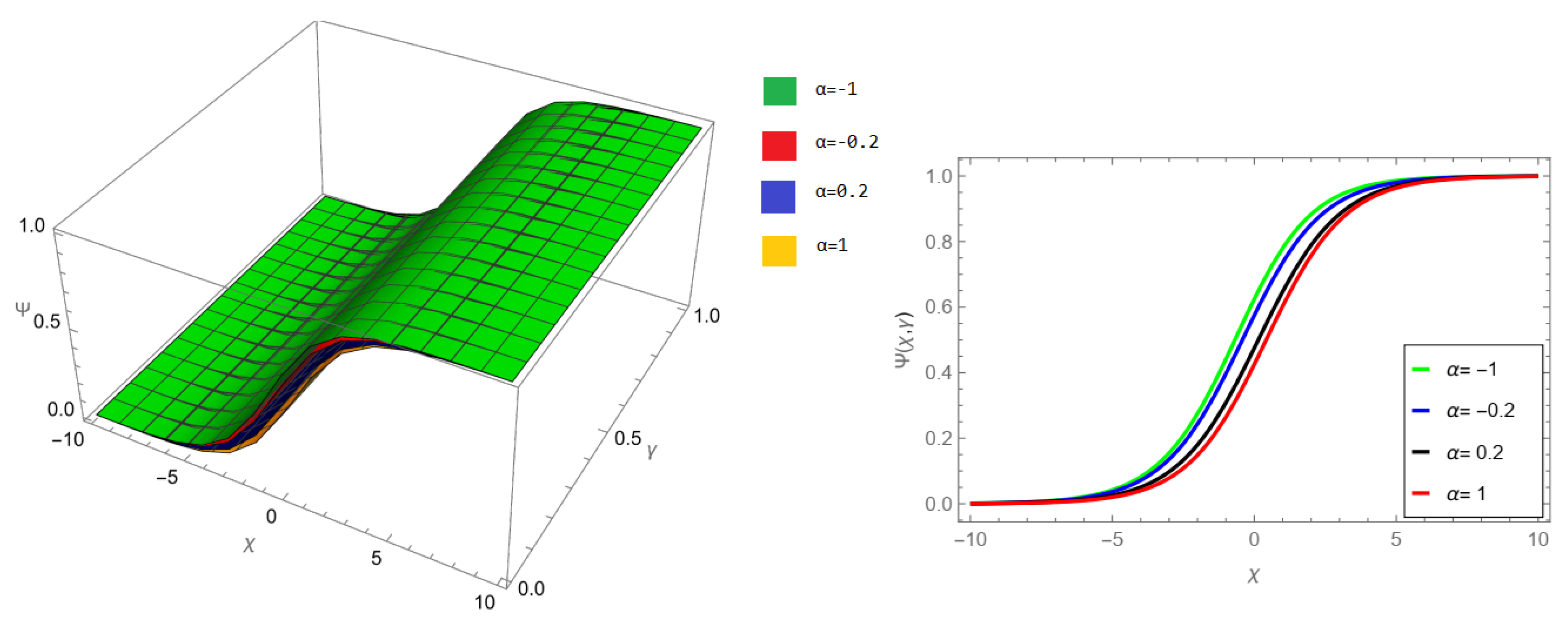
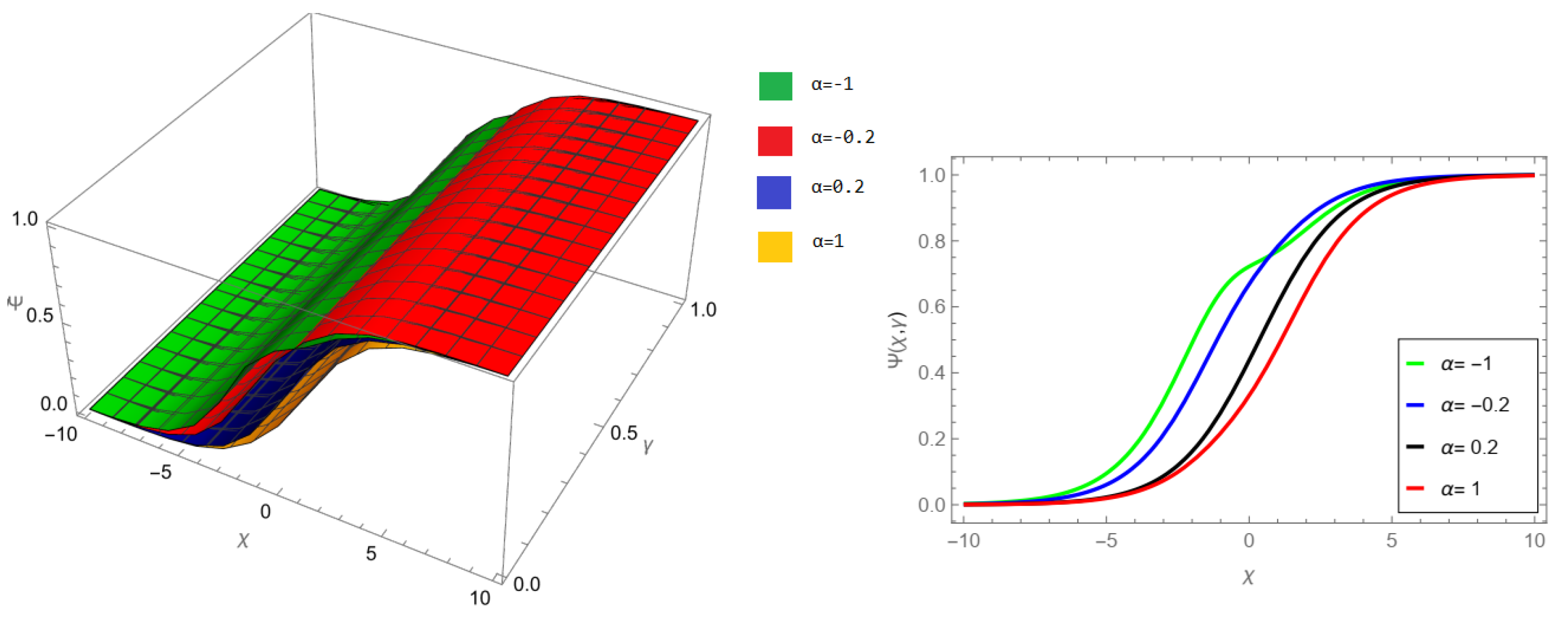
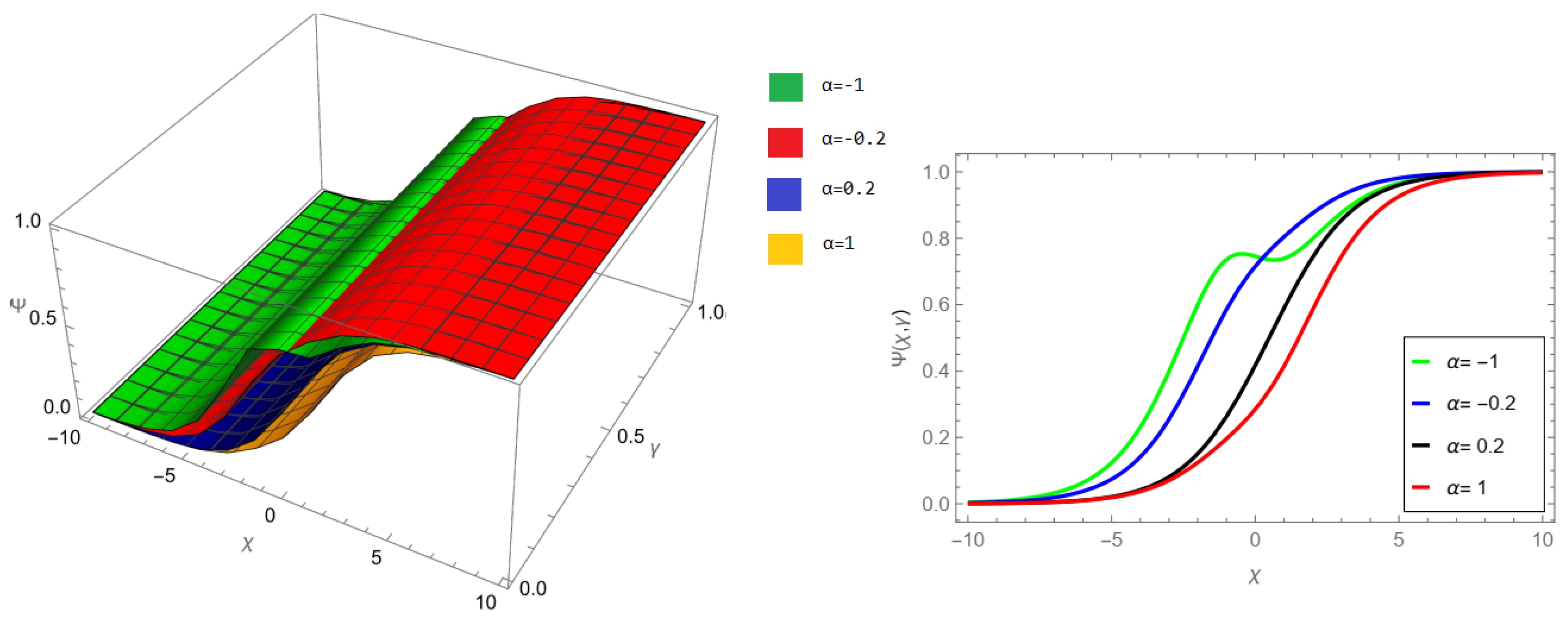
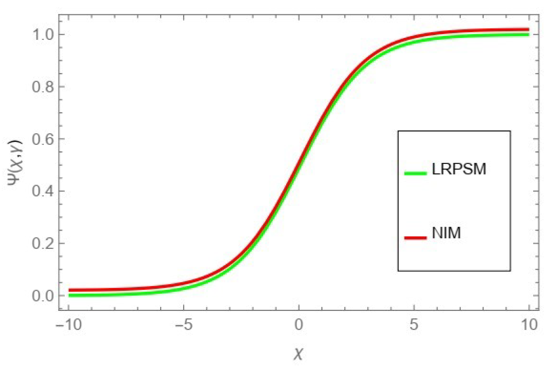
The tables and figures presented in this study provide a comprehensive comparison of the Laplace residual power series method (LRPSM) and the New Iteration Method (NIM) for solving example 1 with varying fractional orders and parameters. Figure 1, LRPSM solution of example 1 for fractional order and . In Figure 2, LRPSM solution of example 1 for fractional order and . Figure 3, LRPSM solution of example 1 for fractional order and . Figure 4, the LRPSM solution of example 1 for fractional order and . Figure 5, LRPSM solution of example 1 for fractional order and . Figure 6, LRPSM solution of example 1 for fractional order and . These figures provide visual insights into the behavior of LRPSM solutions under different fractional orders, offering a clear representation of their convergence characteristics. Figure 7, NIM solution of example 1 for fractional order and . Figure 8, NIM solution of example 1 for fractional order and . Figure 9, NIM solution of example 1 for fractional order and . Figure 10, NIM solution of example 1 for fractional order and . Figure 11, NIM solution of example 1 for fractional order and . Figure 12, NIM solution of example 1 for fractional order and . These visual representations offer insights into the convergence properties and behavior of NIM solutions under different fractional orders. Figure 13, the comparison graph of NIM and LRPSM of fractional order , and . Figure 14, the comparison graph of NIM and LRPSM of fractional order , and . Figure 15, the comparison graph of NIM and LRPSM of fractional order , and .
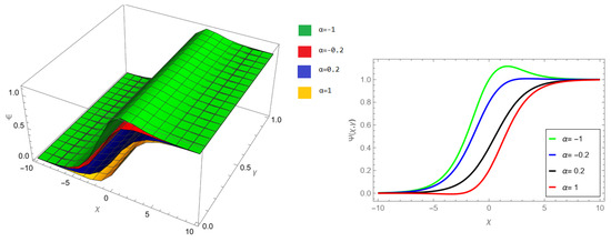
Figure 1.
LRPSM solution of example 1 for fractional order and .
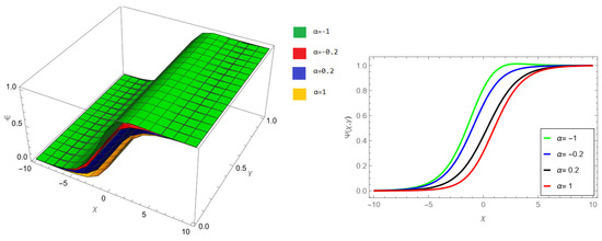
Figure 2.
LRPSM solution of example 1 for fractional order and .
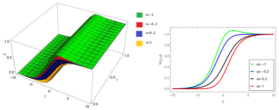
Figure 3.
LRPSM solution of example 1 for fractional order and .
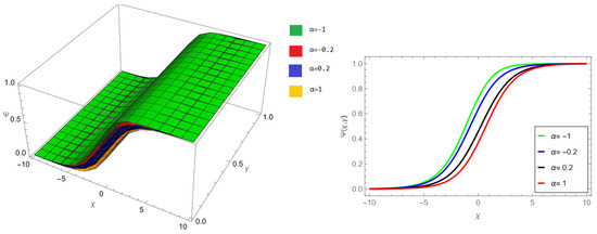
Figure 4.
LRPSM solution of example 1 for fractional order and .
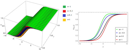
Figure 5.
LRPSM solution of example 1 for fractional order and .
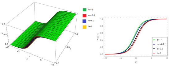
Figure 6.
LRPSM solution of example 1 for fractional order and .
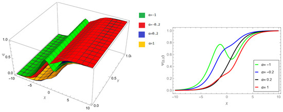
Figure 7.
NIM solution of example 1 for fractional order and .
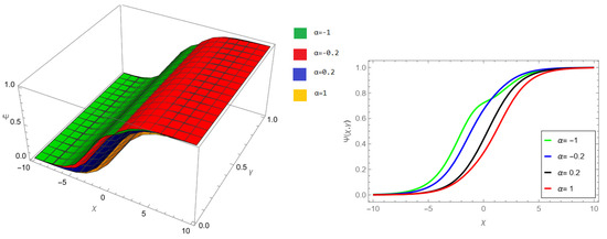
Figure 8.
NIM solution of example 1 for fractional order and .
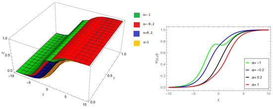
Figure 9.
NIM solution of example 1 for fractional order and .

Figure 10.
NIM solution of example 1 for fractional order and .
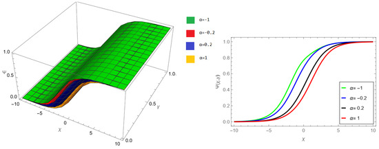
Figure 11.
NIM solution of example 1 for fractional order and .
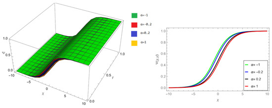
Figure 12.
NIM solution of example 1 for fractional order and .

Figure 13.
The comparison graph of NIM and LRPSM of fractional order , and .
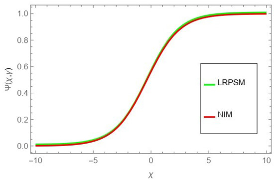
Figure 14.
The comparison graph of NIM and LRPSM of fractional order , and .
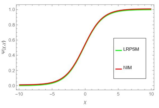
Figure 15.
The comparison graph of NIM and LRPSM of fractional order , and .
Table 1, different fractional-order comparison of LRPSM of example 1 for . Table 2, different fractional-order comparison of LRPSM of example 1 for . Table 3, different fractional-order comparison of LRPSM of example 1 for . Table 1, Table 2 and Table 3 demonstrate the influence of different fractional orders p on the LRPSM solution for , , and , respectively. These tables showcase how changing the fractional order affects the accuracy and convergence of the LRPSM solutions. ’ Table 4, different fractional-order comparison of NIM of example 1 for . Table 5, different fractional-order comparison of NIM of example 1 for . Table 6, different fractional-order comparison of NIM of example 1 for . Table 4, Table 5 and Table 6 present a similar comparative analysis but this time for the New Iteration Method (NIM) with varying fractional orders (). These tables highlight how the choice of fractional order influences the accuracy and efficiency of NIM solutions.

Table 1.
Different fractional-order comparison of LRPSM of example 1 for .
Table 2.
Different fractional-order comparison of LRPSM of example 1 for .
Table 3.
Different fractional-order comparison of LRPSM of example 1 for .
Table 4.
Different fractional-order comparison of NIM of example 1 for .
Table 5.
Different fractional-order comparison of NIM of example 1 for .
Table 6.
Different fractional-order comparison of NIM of example 1 for .
Table 7, the comparison of absolute error for fractional order of LRPSM and NIM. Table 8, the comparison of absolute error for fractional order of LRPSM and NIM. Collectively, these tables and figures provide a comprehensive assessment of the performance of LRPSM and NIM under various fractional orders and parameter settings, aiding researchers and practitioners in choosing the most suitable method for their specific problem and desired level of accuracy.
Table 7.
The comparison of absolute error for fractional order of LRPSM and NIM.
Table 8.
The comparison of absolute error for fractional order of LRPSM and NIM.
7. Conclusions
In conclusion, this study presents a robust and efficient methodology for solving the Fitzhugh-Nagumo equation within the framework of the Caputo operator, combining the Laplace residual power series method (LRPSM) with a novel iteration technique. This approach enhances the accuracy and convergence of solutions, facilitating a deeper understanding of excitable system dynamics. While this research contributes significantly to the field of mathematical modeling and analysis, there are avenues for future work to further expand its impact. One potential direction is the exploration of more intricate excitable systems and their fractional-order counterparts. Additionally, the extension of this methodology to address coupled systems or systems with heterogeneous properties could broaden its applicability. Furthermore, investigating the numerical stability and efficiency of the proposed approach in comparison to other existing methods would be valuable. Overall, these future endeavors aim to solidify and extend the methodology’s utility in understanding complex processes involving fractional calculus.
Funding
This work received support from the Princess Nourah bint Abdulrahman University Researchers Supporting Project number (PNURSP2023R183), Princess Nourah bint Abdulrahman University, Riyadh, Saudi Arabia.
Data Availability Statement
The numerical data used to support the findings of this study are included within the article.
Acknowledgments
This work received support from the Princess Nourah bint Abdulrahman University Researchers Supporting Project number (PNURSP2023R183), Princess Nourah bint Abdulrahman University, Riyadh, Saudi Arabia.
Conflicts of Interest
The authors declare no conflict of interest.
References
- Xiao, J.; Guo, X.; Li, Y.; Wen, S. Further Research on the Problems of Synchronization for Fractional-Order BAM Neural Networks in Octonion-Valued Domain. Neural Process. Lett. 2023, 55, 11173–11208. [Google Scholar] [CrossRef]
- Xiao, J.; Li, Y. Novel synchronization conditions for the unified system of multi-dimension-valued neural networks. Mathematics 2022, 10, 3031. [Google Scholar] [CrossRef]
- Akdemir, A.O.; Butt, S.I.; Nadeem, M.; Ragusa, M.A. New general variants of Chebyshev type inequalities via generalized fractional integral operators. Mathematics 2021, 9, 122. [Google Scholar] [CrossRef]
- Abbas, M.I. Controllability and Hyers-Ulam stability results of initial value problems for fractional differential equations via generalized proportional-Caputo fractional derivative. Miskolc Math. Notes 2021, 22, 491–502. [Google Scholar] [CrossRef]
- Debnath, L. Recent applications of fractional calculus to science and engineering. Int. J. Math. Math. Sci. 2003, 2003, 753601. [Google Scholar] [CrossRef]
- Atangana, A.; Baleanu, D. Caputo-Fabrizio derivative applied to groundwater flow within confined aquifer. J. Eng. Mech. 2017, 143, D4016005. [Google Scholar] [CrossRef]
- Akgul, A.; Khoshnaw, S.A. Application of fractional derivative on non-linear biochemical reaction models. Int. J. Intell. Netw. 2020, 1, 52–58. [Google Scholar] [CrossRef]
- Liu, P.; Shi, J.; Wang, Z.-A. Pattern formation of the attraction-repulsion Keller-Segel system. Discret. Contin. Dyn. Syst. B 2013, 18, 2597–2625. [Google Scholar] [CrossRef]
- Jin, H.; Wang, Z. Boundedness, blowup and critical mass phenomenon in competing chemotaxis. J. Differ. Equ. 2016, 260, 162–196. [Google Scholar] [CrossRef]
- Saad Alshehry, A.; Imran, M.; Weera, W. Fractional View Analysis of Kuramoto-Sivashinsky Equations with Non-Singular Kernel Operators. Symmetry 2022, 14, 1463. [Google Scholar] [CrossRef]
- Alderremy, A.A.; Iqbal, N.; Aly, S.; Nonlaopon, K. Fractional Series Solution Construction for Nonlinear Fractional Reaction-Diffusion Brusselator Model Utilizing Laplace Residual Power Series. Symmetry 2022, 14, 1944. [Google Scholar] [CrossRef]
- Tian, H.; Liu, J.; Wang, Z.; Xie, F.; Cao, Z. Characteristic Analysis and Circuit Implementation of a Novel Fractional-Order Memristor-Based Clamping Voltage Drift. Fractal Fract. 2023, 7, 2. [Google Scholar] [CrossRef]
- Li, Q.; Lin, H.; Tan, X.; Du, S. H∞ Consensus for Multiagent-Based Supply Chain Systems Under Switching Topology and Uncertain Demands. IEEE Trans. Syst. Man. Cybern. Syst. 2020, 50, 4905–4918. [Google Scholar] [CrossRef]
- Dong, J.; Hu, J.; Zhao, Y.; Peng, Y. Opinion formation analysis for Expressed and Private Opinions (EPOs) models: Reasoning private opinions from behaviors in group decision-making systems. Expert Syst. Appl. 2023, 236, 121292. [Google Scholar] [CrossRef]
- Hodgkin, A.L.; Huxley, A.F. A quantitative description of membrane current and its application to conduction and excitation in nerve. J. Physiol. 1952, 117, 500. [Google Scholar] [CrossRef]
- Ozis, T.; Aslan, I. Symbolic computation and construction of new exact traveling wave solutions to Fitzhugh-Nagumo and Klein-Gordon equations. Z. Naturforschung A 2009, 64, 15–20. [Google Scholar] [CrossRef]
- Abbasbandy, S. Soliton solutions for the Fitzhugh-Nagumo equation with the homotopy analysis method. Appl. Math. Model. 2008, 32, 2706–2714. [Google Scholar] [CrossRef]
- Abdusalam, H.A. Analytic and approximate solutions for Nagumo telegraph reaction diffusion equation. Appl. Math. Comput. 2004, 157, 515–522. [Google Scholar] [CrossRef]
- Gurefe, Y.; Sonmezoglu, A.; Misirli, E. Application of the trial equation method for solving some nonlinear evolution equations arising in mathematical physics. Pramana 2011, 77, 1023–1029. [Google Scholar] [CrossRef]
- Bekir, A. New solitons and periodic wave solutions for some nonlinear physical models by using the sine-cosine method. Phys. Scripta 2008, 77, 045008. [Google Scholar] [CrossRef]
- Alquran, M. Solitons and periodic solutions to nonlinear partial differential equations by the Sine-Cosine method. Appl. Math. Inf. Sci. 2012, 6, 85–88. [Google Scholar]
- Marinca, V.; Herisanu, N.; Nemes, I. Optimal homotopy asymptotic method with application to thin film flow. Open Phys. 2008, 6, 648–653. [Google Scholar] [CrossRef]
- Bildik, N.; Deniz, S. New approximate solutions to electrostatic differential equations obtained by using numerical and analytical methods. Georgian Math. J. 2020, 27, 23–30. [Google Scholar] [CrossRef]
- Khader, M.M.; Saad, K.M. A numerical approach for solving the fractional Fisher equation using Chebyshev spectral collocation method. Chaos, Solitons Fractals 2018, 110, 169–177. [Google Scholar] [CrossRef]
- Jafari, H.; Daftardar-Gejji, V. Solving linear and nonlinear fractional diffusion and wave equations by Adomian decomposition. Appl. Math. Comput. 2006, 180, 488–497. [Google Scholar] [CrossRef]
- Atangana, A.; Secer, A. The time-fractional coupled-Korteweg-de-Vries equations. In Abstract and Applied Analysis Hindawi 2013, 2013, 947986. [Google Scholar] [CrossRef]
- Saad, K.M.; Al-Shareef, E.H.; Mohamed, M.S.; Yang, X.J. Optimal q-homotopy analysis method for time-space fractional gas dynamics equation. Eur. Phys. J. Plus 2017, 132, 1–11. [Google Scholar] [CrossRef]
- Saadeh, R.; Alaroud, M.; Al-Smadi, M.; Ahmad, R.R.; Salma Din, U.K. Application of fractional residual power series algorithm to solve Newell-Whitehead-Segel equation of fractional order. Symmetry 2019, 11, 1431. [Google Scholar] [CrossRef]
- Freihet, A.; Hasan, S.; Alaroud, M.; Al-Smadi, M.; Ahmad, R.R.; Salma Din, U.K. Toward computational algorithm for timefractional Fokker-Planck models. Adv. Mech. Eng. 2019, 11, 1–11. [Google Scholar] [CrossRef]
- Al-Smadi, M.; Arqub, O.A.; Hadid, S. Approximate solutions of nonlinear fractional Kundu-Eckhaus and coupled fractional massive Thirring equations emerging in quantum field theory using conformable residual power series method. Phys. Scripta 2020, 95, 105205. [Google Scholar] [CrossRef]
- Al-Smadi, M.; Arqub, O.A.; Momani, S. Numerical computations of coupled fractional resonant Schrodinger equations arising in quantum mechanics under conformable fractional derivative sense. Phys. Scripta 2020, 95, 075218. [Google Scholar] [CrossRef]
- Al-Smadi, M.; Arqub, O.A.; Hadid, S. An attractive analytical technique for coupled system of fractional partial differential equations in shallow water waves with conformable derivative. Commun. Theor. Phys. 2020, 72, 085001. [Google Scholar] [CrossRef]
- Alaroud, M.; Al-smadi, M.; Ahmad, R.R.; Salma Din, U.K. Numerical computation of fractional Fredholm integrodifferential equation of order 2b arising in natural sciences. J. Phys. Conf. Ser. 2019, 1212, 012022. [Google Scholar] [CrossRef]
- Alaroud, M.; Al-Smadi, M.; Ahmad, R.R.; Salma Din, U.K. An Analytical Numerical Method for Solving Fuzzy Fractional Volterra Integro-Differential Equations. Symmetry 2019, 11, 205. [Google Scholar] [CrossRef]
- Komashynska, I.; Al-Smadi, M.; Arqub, O.A.; Momani, S. An efficient analytical method for solving singular initial value problems of nonlinear systems. Appl. Math. Inform. Sci. 2016, 10, 647–656. [Google Scholar] [CrossRef]
- Jawarneh, Y.; Yasmin, H.; Al-Sawalha, M.M.; Khan, A. Numerical analysis of fractional heat transfer and porous media equations within Caputo-Fabrizio operator. AIMS Math. 2023, 8, 26543–26560. [Google Scholar] [CrossRef]
- Jawarneh, Y.; Yasmin, H.; Al-Sawalha, M.M.; Khan, A. Fractional comparative analysis of Camassa-Holm and Degasperis-Procesi equations. AIMS Math. 2023, 8, 5845–25862. [Google Scholar] [CrossRef]
- Liaqat, M.I.; Okyere, E. Comparative Analysis of the Time-Fractional Black-Scholes Option Pricing Equations (BSOPE) by the Laplace Residual Power Series Method (LRPSM). J. Math. 2023, 2023, 6092283. [Google Scholar] [CrossRef]
- Shafee, A.; Alkhezi, Y.; Shah, R. Efficient Solution of Fractional System Partial Differential Equations Using Laplace Residual Power Series Method. Fractal Fract. 2023, 7, 429. [Google Scholar] [CrossRef]
- Albalawi, W.; Shah, R.; Nonlaopon, K.; El-Sherif, L.S.; El-Tantawy, S.A. Laplace Residual Power Series Method for Solving Three-Dimensional Fractional Helmholtz Equations. Symmetry 2023, 15, 194. [Google Scholar] [CrossRef]
- Al-Sawalha, M.M.; Yasmin, H.; Ganie, A.H.; Moaddy, K. Unraveling the Dynamics of Singular Stochastic Solitons in Stochastic Fractional Kuramoto-Sivashinsky Equation. Fractal Fract. 2023, 7, 753. [Google Scholar] [CrossRef]
- Bhalekar, S.; Daftardar-Gejji, V. New iterative method: Application to partial differential equations. Appl. Math. Comput. 2008, 203, 778–783. [Google Scholar] [CrossRef]
- El-Ajou, A. Adapting the Laplace transform to create solitary solutions for the nonlinear time-fractional dispersive PDEs via a new approach. Eur. Phys. J. Plus 2021, 136, 1–22. [Google Scholar] [CrossRef]
- Alquran, M.; Ali, M.; Alsukhour, M.; Jaradat, I. Promoted residual power series technique with Laplace transform to solve some time-fractional problems arising in physics. Results Phys. 2020, 19, 103667. [Google Scholar] [CrossRef]
- Daftardar-Gejji, V.; Jafari, H. An iterative method for solving nonlinear functional equations. J. Math. Anal. Appl. 2006, 316, 753–763. [Google Scholar] [CrossRef]
- Bhalekar, S.; Daftardar-Gejji, V. Convergence of the new iterative method. Int. J. Differ. Equ. 2011, 2011, 989065. [Google Scholar] [CrossRef]


Disclaimer/Publisher’s Note: The statements, opinions and data contained in all publications are solely those of the individual author(s) and contributor(s) and not of MDPI and/or the editor(s). MDPI and/or the editor(s) disclaim responsibility for any injury to people or property resulting from any ideas, methods, instructions or products referred to in the content. |
© 2023 by the author. Licensee MDPI, Basel, Switzerland. This article is an open access article distributed under the terms and conditions of the Creative Commons Attribution (CC BY) license (https://creativecommons.org/licenses/by/4.0/).