Explicit Soliton Structure Formation for the Riemann Wave Equation and a Sensitive Demonstration

Abstract

The motive of the study was to explore the nonlinear Riemann wave equation, which describes the tsunami and tidal waves in the sea and homogeneous and stationary media. This study establishes the framework for the analytical solutions to the Riemann wave equation using the new extended direct algebraic method. As a result, the soliton patterns of the Riemann wave equation have been successfully illustrated, with exact solutions offered by the plane solution, trigonometry solution, mixed hyperbolic solution, mixed periodic and periodic solutions, shock solution, mixed singular solution, mixed trigonometric solution, mixed shock single solution, complex soliton shock solution, singular solution, and shock wave solutions. Graphical visualization is provided of the results with suitable values of the involved parameters by Mathematica. It was visualized that the velocity of the soliton and the wave number controls the behavior of the soliton. We are confident that our research will assist physicists in predicting new notions in mathematical physics.

1. Introduction

The nonlinear partial differential equation is critical for investigating the characteristics of nonlinear physical events. The Schrödinger governing equation is a one-of-a-kind mechanism for appropriately understanding the complicated physical nonlinear model, with vital applications in plasma, fiber optics, telecommunication engineering, mathematical physics, and optics. Obtaining reliable analytical solutions for the Schrödinger equations is an essential research topic since exact solutions represent the physical features of nonlinear systems in applied mathematics [1,2,3,4,5,6,7,8]. Nonlinear partial differential equations (PDEs) have increased in popularity and importance in both applied and pure mathematics during the last decade. For mathematicians, computer technology has expanded the scope of applied sciences. Nonlinear models are becoming increasingly prevalent in mathematical physics and engineering sciences. PDEs are generally used to create mathematical models of important tangible phenomena in various nonlinear sciences and engineering areas. Nonlinear PDEs have a wide range of practical applications, including mass and heat transportation, continuum mechanics, wave theory, hydrodynamics, chemical technology, acoustics and plasma physics [9,10,11,12,13], biology [14,15], population ecology [16], plasma waves [17], civil engineering [18], quantum mechanics [19,20,21], and so on. In geographical fields, regarding environmental processes induced by energy transportation on floating or synthetic structure fields, waves are primary energy sources.

The mathematical explanation includes the discovery of solitons, the great diversity of the structure, and its essential features. The story of solitons begins with an observation of the translation wave made by John Scott Russell. Before the 1870s, when Russell’s work was eventually proven, notable scientists and philosophers praised its scientific implications. Boussinesq’s 1872 work was practiced extensively and it predicted major concepts that are employed today involving forward-thinking scientists and philosophers. Boussinesq expressed his opinion on the water wave equation. As a result, his estimate suggests that the movement may be a duplex. However, Boussinesq and Rayleigh’s work still prove the essential issues of dispersion and non-linearity. The Stokes–Airy argument against making an equation of unidirectional motion is still rendering; it is now recognized by their names by using bell-shaped and kink-shaped sech-solutions, simulating wave phenomena in plasma, optical fiber, elastic media, chemical electrical circuits, and other fields. The traveling wave solutions of the Boussinesq and Korteweg de Vries equations, which describe water waves, are well-known examples. For more information, see [22,23,24,25,26,27].

Many schemes and approaches, such as the Kudryashov method [28], sine-Gordon expansion scheme [29], bilinear neural network technique [30], and a simple extended equation method [31], have been developed to secure exact analytical solutions for partial nonlinear differential equations to find soliton solutions, [32] F-expansion technique [33], unified auxiliary equation technique (m + $\frac{G}{G^{{}^{\prime }}}$) expansion strategy [34], Hirota bilinear technique [35], extended exponential function method [36], generalized exponential rational function method [37], variational iteration method [38], and several others [39,40,41,42,43,44,45,46].

In this paper, we used a new algebraic extended approach to identify broad-ranging solitary wave solutions to the Riemann wave equation. In the geographical fields, regarding environmental processes induced by energy transportation on floating or synthetic structure fields, waves are the primary energy sources. The Riemann wave equation is a nonlinear equation used in studying tidal and tsunami waves in seas and rivers, homogeneous and stationary media, ion and magneto-sound waves in plasma, electromagnetic waves in power lines, marine and coastal engineering, and other fields. This study establishes the framework for the analytical solutions to the Riemann wave equation using the new algebraic extended method. The soliton patterns of the Riemann wave equation have been successfully illustrated, with exact solutions offered by the plane solution, trigonometry solution, mixed hyperbolic solution, mixed periodic and periodic solutions, shock solution, singular solution, mixed singular solution, mixed trigonometric solution, mixed shock single solution, complex solitary shock solution, and shock wave solutions. The survey results are compared to the highly recognized results and the results are presented. Graphical comparisons are provided for the Riemann wave equation model solutions, which are presented diagrammatically by adjusting the values of the embedded parameters in Mathematica. For accuracy, the results are visually displayed in 3D, contour, and 2D. We also demonstrated the sensitivity analysis for the redesigned dynamical structural system wave profiles, where the soliton wave velocity and wave number parameters regulate the water wave singularity. We are confident that our research will assist physicists in predicting new notions in mathematical physics. The Riemann coupled wave system of equations is given as [47],

$$\begin{array}{c}\hfill \begin{array}{cc}& \frac{\partial \mathcal{U}}{\partial t}+f\frac{\partial {\mathcal{U}}^3}{\partial x^2\partial y}+j\mathcal{U}\frac{\partial \mathcal{V}}{\partial x}+k\mathcal{V}\frac{\partial \mathcal{W}}{\partial x}=0,\hfill \\ & \frac{\partial \mathcal{U}}{\partial x}=\frac{\partial \mathcal{V}}{\partial x},\hfill \end{array}\end{array}$$

(1)

where f, j, and k are non-zero parameters, Equation (1) explains the (2 + 1)-dimensional interaction of a Riemann wave traveling down the y-axis with a long wave propagating along the x-axis. These equations are fully integrable and have extensive applications in ocean tsunamis and tidal wave propagation. Another significant aspect of Equation (1) describes the turbulent state by combining whistling wave packets featuring random phases with limited amplitude. Whistler turbulence interferes with the magnetic sound wave, damping it and, hence, the electrostatic wave in the plasma [48].

The extraction of analytical solutions to partial differential equations by using the various analytical methodologies is a significant and attractive field of mathematical physics. It has lately emerged as the most fascinating and exciting field of research. The exact solutions to these equations should be examined while researching the physical processes of natural occurrences defined. In the literature, there are a few common strategies for finding accurate solutions to the integrable Riemann wave equation [49,50,51,52,53,54,55,56,57]. As a result, we desire to employ the new algebraic extended method to provide inclusive, standard, substantial, and understandable soliton structured solutions to Riemann wave equations that are confined in all (2 + 1)-dimensional directions.

Recently, in December 2022, Attaullah et al. [47] investigated the Riemann wave Equation (1) in solitons. The modified Exp function method was applied to the considered model and obtained dark, periodic, and logarithmic analytical soliton solutions. The modified Exp function provides only five different families of solutions. Indeed, solutions are correct but many types of soliton solutions are not found for the Riemann wave equation and the sensitivity analysis of the considered model is a gap. This ongoing study inspired us to perform this work. The new extended direct algebraic method is one of the generalized methods that provides twelve different families along with thirty-seven soliton solutions in which dark, bright, singular, rational, plane solution, trigonometry solution, mixed hyperbolic solution, mixed periodic and periodic solutions, shock solution, singular solution, mixed singular solution, mixed trigonometric solution, mixed shock single solution, complex solitary shock solution, and shock wave solutions are included. The other thing is the sensitivity analysis, which was not previously done with the Riemann wave equation. The sensitive visualization of the model is presented and visualized on different initial conditions and attempts to fill this study gap.

The core purpose of this research is to cast aspersions on the projected Riemann wave equation model. To obtain an exact analytical solution, a new extended direct algebraic method was used. We begin with a basic explanation and define the famous Riemann wave equation governing model. In Section 2, we construct analytical solutions using the new extended direct algebraic method. The description of method mentioned. The application of the new extended direct algebraic method is shown in Section 2. Furthermore, for different values of wave velocity, we see diverse wave textures in the 3D, contour, and 2D graphical depictions of the solutions. We discuss the visual representation of the study findings in Section 3. Section 4 presents the sensitivity assessment for the wave velocity profiles graphically with the discussions and results analysis. The study’s conclusion is given in Section 5.

2. Structures of Analytical Solutions

2.1. New Extended Direct Algebraic Method

The new extended direct algebraic equation method is a generalized technique that provides thirty-seven soliton solutions with twelve different families. The analytical exact solutions that came up with this approach contain, for example, trigonometric, hyperbolic–trigonometric, rational, logarithmic, and periodic solutions.

Assume a general NPDE (nonlinear partial differential equation) of the type:

$$\begin{array}{c}\hfill Y(\Omega ,{\Omega }_t,{\Omega }_x,{\Omega }_{tt},{\Omega }_{xx},\cdots )=0.\end{array}$$

(2)

The ordinary differential equation can be obtained as follows:

$$\begin{array}{c}\hfill \mathcal{Q}(\mathbb{E},{\mathbb{E}}^{\prime },{\mathbb{E}}^{″},\cdots )=0,\end{array}$$

(3)

by the mean of transformation, which is given below,

$$\mathsf{\Omega }(x,y,z,t)=\mathbb{E}\left(\xi \right),$$

(4)

where $\xi =k_{1}x+k_{2}y+k_{3}t$ and $k_1, k_2, k_3$ are real constant. It can be modified according to the physical phenomenon. Consider the following solution of Equation (3):

$$\begin{array}{c}\hfill \mathbb{E}\left(\xi \right)=\sum _{j=0}^m\left[b_j{\left(\eta \left(\xi \right)\right)}^j\right],\end{array}$$

(5)

along with,

$$\begin{array}{c}\hfill {\eta }^{{}^{\prime }}\left(\xi \right)=\alpha ln\left(A\right)+\beta S\left(\xi \right)ln\left(A\right)+\gamma {\left(S\left(\xi \right)\right)}^{2}ln\left(A\right),\end{array}$$

where $\alpha$, $\beta$ and $\gamma$ are real constants and $\mathfrak{S}={\beta }^2-4\alpha \gamma$. The general solutions concerning the parameters $\alpha$, $\beta$ and $\gamma$ are:

(Family 1): When $\gamma \ne 0,$ and ${\beta }^2-4\alpha \gamma <0$,

$$\begin{array}{lllllllll}{\eta }_1\left(\xi \right)\hfill & =& -\frac{\beta }{2\gamma }+\frac{\sqrt{-\mathfrak{S}}}{2\gamma }{tan}_{\chi }\left(\frac{\sqrt{-\mathfrak{S}}}{2}\xi \right),\hfill & & & & & & \end{array}$$

(6)

$$\begin{array}{ccccccccc}{\eta }_2\left(\xi \right)\hfill & =& -\frac{\beta }{2\gamma }-\frac{\sqrt{-\mathfrak{S}}}{2\gamma }{cot}_{\chi }\left(\frac{\sqrt{-\mathfrak{S}}}{2}\xi \right),\hfill & & & & & & \end{array}$$

(7)

$$\begin{array}{ccc}{\eta }_3\left(\xi \right)\hfill & =& -\frac{\beta }{2\gamma }+\frac{\sqrt{-\mathfrak{S}}}{2\gamma }\left({tan}_{\chi }\left(\sqrt{-\mathfrak{S}}\xi \right)\pm \sqrt{mn}{sec}_{\chi }\left(\sqrt{-\mathfrak{S}}\xi \right)\right),\hfill \end{array}$$

(8)

$$\begin{array}{ccc}{\eta }_4\left(\xi \right)\hfill & =& -\frac{\beta }{2\gamma }+\frac{\sqrt{-\mathfrak{S}}}{2\gamma }\left({cot}_{\chi }\left(\sqrt{-\mathfrak{S}}\xi \right)\pm \sqrt{mn}{csc}_{\chi }\left(\sqrt{-\mathfrak{S}}\xi \right)\right),\hfill \end{array}$$

(9)

$$\begin{array}{ccc}{\eta }_5\left(\xi \right)\hfill & =& -\frac{\beta }{2\gamma }+\frac{\sqrt{-\mathfrak{S}}}{4\gamma }\left({tan}_{\chi }\left(\frac{\sqrt{-\mathfrak{S}}}{4}\xi \right)-{cot}_{\chi }\left(\frac{\sqrt{-\mathfrak{S}}}{4}\xi \right)\right).\hfill \end{array}$$

(10)

(Family 2): When $\gamma \ne 0$ and ${\beta }^2-4\alpha \gamma >0$,

$$\begin{array}{ccccccccc}\hfill {\eta }_6\left(\xi \right)& =& -\frac{\beta }{2\gamma }-\frac{\sqrt{\mathfrak{S}}}{2\gamma }{tanh}_{\chi }\left(\frac{\sqrt{\mathfrak{S}}}{2}\xi \right),\hfill & & & & & & \end{array}$$

(11)

$$\begin{array}{ccccccccc}\hfill {\eta }_7\left(\xi \right)& =& -\frac{\beta }{2\gamma }-\frac{\sqrt{\mathfrak{S}}}{2\gamma }{coth}_{\chi }\left(\frac{\sqrt{\mathfrak{S}}}{2}\xi \right),\hfill & & & & & & \end{array}$$

(12)

$$\begin{array}{ccc}\hfill {\eta }_8\left(\xi \right)& =& -\frac{\beta }{2\gamma }+\frac{\sqrt{\mathfrak{S}}}{2\gamma }\left(-{tanh}_{\chi }\left(\sqrt{\mathfrak{S}}\xi \right)\pm i\sqrt{mn}sec{h}_{\chi }\left(\sqrt{\mathfrak{S}}\xi \right)\right),\hfill \end{array}$$

(13)

$$\begin{array}{ccc}\hfill {\eta }_9\left(\xi \right)& =& -\frac{\beta }{2\gamma }+\frac{\sqrt{\mathfrak{S}}}{2\gamma }\left(-{coth}_{\chi }\left(\sqrt{\mathfrak{S}}\xi \right)\pm \sqrt{mn}csc{h}_{\chi }\left(\sqrt{\mathfrak{S}}\xi \right)\right),\hfill \end{array}$$

(14)

$$\begin{array}{ccc}\hfill {\eta }_{10}\left(\xi \right)& =& -\frac{\beta }{2\gamma }-\frac{\sqrt{\mathfrak{S}}}{4\gamma }\left(tan{h}_{\chi }\left(\frac{\sqrt{\mathfrak{S}}}{4}\xi \right)+cot{h}_{\chi }\left(\frac{\sqrt{\mathfrak{S}}}{4}\xi \right)\right).\hfill \end{array}$$

(15)

(Family 3): When $\beta =0$ and $\alpha \gamma >0$,

$$\begin{array}{ccccccccc}\hfill {\eta }_{11}\left(\xi \right)& =& \sqrt{\frac{\alpha }{\gamma }}ta{n}_{\chi }\left(\sqrt{\alpha \gamma }\xi \right),\hfill & & & & & & \end{array}$$

(16)

$$\begin{array}{ccccccccc}\hfill {\eta }_{12}\left(\xi \right)& =& -\sqrt{\frac{\alpha }{\gamma }}co{t}_{\chi }\left(\sqrt{\alpha \gamma }\xi \right),\hfill & & & & & & \end{array}$$

(17)

$$\begin{array}{ccc}\hfill {\eta }_{13}\left(\xi \right)& =& \sqrt{\frac{\alpha }{\gamma }}\left({tan}_{\chi }\left(2\sqrt{\alpha \gamma }\xi \right)\pm \sqrt{mn}se{c}_{\chi }\left(2\sqrt{\alpha \gamma }\xi \right)\right),\hfill \end{array}$$

(18)

$$\begin{array}{ccc}\hfill {\eta }_{14}\left(\xi \right)& =& \sqrt{\frac{\alpha }{\gamma }}\left(-co{t}_{\chi }\left(2\sqrt{\alpha \gamma }\xi \right)\pm \sqrt{mn}{csc}_{\chi }\left(2\sqrt{\alpha \gamma }\xi \right)\right),\hfill \end{array}$$

(19)

$$\begin{array}{cccc}\hfill {\eta }_{15}\left(\xi \right)& =& \frac{1}{2}\sqrt{\frac{\alpha }{\gamma }}\left({tan}_{\chi }\left(\frac{\sqrt{\alpha \gamma }}{2}\xi \right)-{cot}_{\chi }\left(\frac{\sqrt{\alpha \gamma }}{2}\xi \right)\right).\hfill & \end{array}$$

(20)

(Family 4): When $\beta =0$ and $\alpha \gamma <0$,

$$\begin{array}{cccccccccc}\hfill {\eta }_{16}\left(\xi \right)& =& -\sqrt{-\frac{\alpha }{\gamma }}{tanh}_{\chi }\left(\sqrt{-\alpha \gamma }\xi \right),\hfill & & & & & & & \end{array}$$

(21)

$$\begin{array}{cccccccccc}\hfill {\eta }_{17}\left(\xi \right)& =& -\sqrt{-\frac{\alpha }{\gamma }}{coth}_{\chi }\left(\sqrt{-\alpha \gamma }\xi \right),\hfill & & & & & & & \end{array}$$

(22)

$$\begin{array}{cccc}& \hfill {\eta }_{18}\left(\xi \right)& =& \sqrt{-\frac{\alpha }{\gamma }}\left(-{tanh}_{\chi }\left(2\sqrt{-\alpha \gamma }\xi \right)\pm i\sqrt{mn}sec{h}_{\chi }\left(2\sqrt{-\alpha \gamma }\xi \right)\right),\hfill \end{array}$$

(23)

$$\begin{array}{ccc}\hfill {\eta }_{19}\left(\xi \right)& =& \sqrt{-\frac{\alpha }{\gamma }}\left(-{coth}_{\chi }\left(2\sqrt{-\alpha \gamma }\xi \right)\pm \sqrt{mn}csc{h}_{\chi }\left(2\sqrt{-\alpha \gamma }\xi \right)\right),\hfill \end{array}$$

(24)

$$\begin{array}{cccc}\hfill {\eta }_{20}\left(\xi \right)& =& -\frac{1}{2}\sqrt{-\frac{\alpha }{\gamma }}\left({tanh}_{\chi }\left(\frac{\sqrt{-\alpha \gamma }}{2}\xi \right)+cot{h}_{\chi }\left(\frac{\sqrt{-\alpha \gamma }}{2}\xi \right)\right).\hfill & \end{array}$$

(25)

(Family 5): When $\alpha =\gamma$ and $\beta =0$,

$$\begin{array}{ccccccccc}\hfill {\eta }_{21}\left(\xi \right)& =& {tan}_{\chi }\left(\alpha \xi \right),\hfill & & & & & & \end{array}$$

(26)

$$\begin{array}{cccccccc}\hfill {\eta }_{22}\left(\xi \right)& =& -{cot}_{\chi }\left(\alpha \xi \right),\hfill & & & & & \end{array}$$

(27)

$$\begin{array}{cccc}\hfill {\eta }_{23}\left(\xi \right)& =& {tan}_{\chi }\left(2\alpha \xi \right)\pm \sqrt{mn}{sec}_{\chi }\left(2\alpha \xi \right),\hfill & \end{array}$$

(28)

$$\begin{array}{ccc}\hfill {\eta }_{24}\left(\xi \right)& =& -{cot}_{\chi }\left(2\alpha \xi \right)\pm \sqrt{mn}{csc}_{\chi }\left(2\alpha \xi \right),\hfill \end{array}$$

(29)

$$\begin{array}{cccc}\hfill {\eta }_{25}\left(\xi \right)& =& \frac{1}{2}\left({tan}_{\chi }\left(\frac{\alpha }{2}\xi \right)-{cot}_{\chi }\left(\frac{\alpha }{2}\xi \right)\right).\hfill & \end{array}$$

(30)

(Family 6): When $\alpha =-\gamma$ and $\beta =0$,

$$\begin{array}{ccccccccc}\hfill {\eta }_{26}\left(\xi \right)& =& -{tanh}_{\chi }\left(\alpha \xi \right),\hfill & & & & & & \end{array}$$

(31)

$$\begin{array}{ccccccccc}\hfill {\eta }_{27}\left(\xi \right)& =& -{coth}_{\chi }\left(\alpha \xi \right),\hfill & & & & & & \end{array}$$

(32)

$$\begin{array}{ccc}\hfill {\eta }_{28}\left(\xi \right)& =& -{tanh}_{\chi }\left(2\alpha \xi \right)\pm i\sqrt{mn}sec{h}_{\chi }\left(2\alpha \xi \right),\hfill \end{array}$$

(33)

$$\begin{array}{cccc}\hfill {\eta }_{29}\left(\xi \right)& =& -{cot}_{\chi }\left(2\alpha \xi \right)\pm \sqrt{mn}csc{h}_{\chi }\left(2\alpha \xi \right),\hfill & \end{array}$$

(34)

$$\begin{array}{ccc}\hfill {\eta }_{30}\left(\xi \right)& =& -\frac{1}{2}\left({tanh}_{\chi }\left(\frac{\alpha }{2}\xi \right)+{coth}_{\chi }\left(\frac{\alpha }{2}\xi \right)\right).\hfill \end{array}$$

(35)

(Family 7): When ${\beta }^2=4\alpha \gamma$,

$$\begin{array}{c}\hfill {\eta }_{31}\left(\xi \right)=\frac{-2\alpha (\beta \xi log[\chi ]+2)}{{\beta }^2\xi log\left[\chi \right]}.\end{array}$$

(36)

(Family 8): When $\alpha =pq,(q\ne 0)$, $\gamma =0$ and $\beta =p,$

$$\begin{array}{c}\hfill {\eta }_{32}\left(\xi \right)={\chi }^{p\xi }-q.\end{array}$$

(37)

(Family 9): When $\gamma =\beta =0$,

$$\begin{array}{c}\hfill {\eta }_{33}\left(\xi \right)=\alpha \xi log\left[\chi \right].\end{array}$$

(38)

(Family 10): When $\alpha =\beta =0$,

$$\begin{array}{c}\hfill {\eta }_{34}\left(\xi \right)=\frac{-1}{\gamma \xi log\left[\chi \right]}.\end{array}$$

(39)

(Family 11): When $\beta \ne 0$ and $\alpha =0$,

$$\begin{array}{c}\hfill {\eta }_{35}\left(\xi \right)=-\frac{m\beta }{\gamma \left({cosh}_{\chi }\left(\beta \xi \right)-{sinh}_{\chi }\left(\beta \xi \right)+m\right)},\end{array}$$

(40)

$$\begin{array}{c}\hfill {\eta }_{36}\left(\xi \right)=-\frac{\beta \left({sinh}_{\chi }\left(\beta \xi \right)+{cosh}_{\chi }\left(\beta \xi \right)\right)}{\gamma \left({sinh}_{\chi }\left(\beta \xi \right)+{cosh}_{\chi }\left(\beta \xi \right)+n\right)}.\end{array}$$

(41)

(Family 12): When $\gamma =pq,(q\ne 0)$, $\alpha =0$ and $\beta =p$,

$$\begin{array}{c}\hfill {\eta }_{37}\left(\xi \right)=-\frac{m{\chi }^{p\xi }}{m-qn{\chi }^{p\xi }},\end{array}$$

(42)

$$\begin{array}{c}\hfill {sinh}_{\chi }\left(\xi \right)=\frac{m{\chi }^{\xi }-n{\chi }^{-\xi }}{2},{cosh}_{\chi }\left(\xi \right)=\frac{m{\chi }^{\xi }+n{\chi }^{-\xi }}{2},\end{array}$$

$$\begin{array}{c}\hfill {tanh}_{\chi }\left(\xi \right)=\frac{m{\chi }^{\xi }-n{\chi }^{-\xi }}{m{\chi }^{\xi }+n{\chi }^{-\xi }},{coth}_{\chi }\left(\xi \right)=\frac{m{\chi }^{\xi }+n{\chi }^{-\xi }}{m{\chi }^{\xi }-n{\chi }^{-\xi }},\end{array}$$

$$\begin{array}{c}\hfill sec{h}_{\chi }\left(\xi \right)=\frac{2}{m{\chi }^{\xi }+n{\chi }^{-\xi }},csc{h}_{\chi }\left(\xi \right)=\frac{2}{m{\chi }^{\xi }-n{\chi }^{-\xi }},\end{array}$$

$$\begin{array}{c}\hfill si{n}_{\chi }\left(\xi \right)=\frac{m{\chi }^{i\xi }-n{\chi }^{-i\xi }}{2i},co{\eta }_{\chi }\left(\xi \right)=\frac{m{\chi }^{i\xi }+n{\chi }^{-i\xi }}{2},\end{array}$$

$$\begin{array}{c}\hfill {tan}_{\chi }\left(\xi \right)=-i\frac{m{\chi }^{i\xi }-n{\chi }^{-i\xi }}{m{\chi }^{i\xi }+n{\chi }^{-i\xi }},{cot}_{\chi }\left(\xi \right)=i\frac{m{\chi }^{i\xi }+n{\chi }^{-i\xi }}{m{\chi }^{i\xi }-n{\chi }^{-i\xi }},\end{array}$$

where $n,m>0$ are parameters of arbitrary constant deformations.

2.2. Application of the New Extended Direct Algebraic Method

In order to find the analytical exact solution of the Riemann wave equation, the next wave transformation was applied to the system (1),

$$\begin{array}{c}\hfill \mathcal{U}(x,y,t)=\mathcal{U}\left(\xi \right),\mathcal{V}(x,y,t)=\mathcal{V}\left(\xi \right),\xi =(\lambda x+\omega y-ct),\end{array}$$

(43)

where c is the wave velocity of the traveling wave while $\lambda$ and $\omega$ are wave numbers.

$$\begin{array}{c}\hfill \begin{array}{cc}& \omega f{\lambda }^2\frac{d\mathcal{U}}{d{\xi }^3}+j\lambda \mathcal{U}\frac{d\mathcal{V}}{d\xi }+k\mathcal{V}\frac{d\mathcal{V}}{d\xi }=0,\hfill \\ & \omega \frac{d\mathcal{U}}{d\xi }=\lambda \frac{d\mathcal{V}}{d\xi }.\hfill \end{array}\end{array}$$

(44)

Integrating the second equation of system (44) with zero constants of integration we have

$$\begin{array}{c}\hfill \mathcal{V}=\frac{\omega }{\lambda }\mathcal{U}.\end{array}$$

(45)

Substituting Equation (45) into the first system of Equation (44) after integration, we have

$$\begin{array}{c}\hfill 2\omega f{\lambda }^2\frac{d{\mathcal{U}}^2}{d{\xi }^2}+\omega (j+k){\mathcal{U}}^2-2c\mathcal{U}=0.\end{array}$$

(46)

The homogeneous balancing constant of Equation (46) is $m=2$. Thus, the general solution (5) is expanded by using $m=2$ for Equation (46), so the solution is given as,

$$\begin{array}{c}\hfill \mathcal{U}\left(\xi \right)=b_0+b_1\eta \left(\xi \right)+b_2{\eta }^2\left(\xi \right),\end{array}$$

(47)

where

$$\begin{array}{c}\hfill {\eta }^{{}^{\prime }}\left(\xi \right)=\alpha ln\left(A\right)+\beta S\left(\xi \right)ln\left(A\right)+\gamma {\left(S\left(\xi \right)\right)}^{2}ln\left(A\right).\end{array}$$

(48)

Equation (47) is substituted in Equation (46). We obtain the algebraic system by equating the coefficients of distinct powers of $\eta \left(\xi \right)$,

$$\begin{array}{c}\hfill \begin{array}{cc}\hfill \eta {\left(\xi \right)}^0:& 2\omega f{\lambda }^2{b}_1\beta {\left(ln\left(A\right)\right)}^2\alpha +\omega k{b_0}^2+\omega j{b_0}^2-2c{b}_0+4\omega f{\lambda }^2{b}_2{\alpha }^2{\left(ln\left(A\right)\right)}^2=0,\hfill \\ \hfill \eta {\left(\xi \right)}^1:& 4\omega f{\lambda }^2{b}_1\gamma {\left(ln\left(A\right)\right)}^2\alpha +12\omega f{\lambda }^2{b}_2\alpha {\left(ln\left(A\right)\right)}^2\beta +2\omega f{\lambda }^2{b}_1{\beta }^2{\left(ln\left(A\right)\right)}^2-\hfill \\ & 2c{b}_1+2\omega j{b}_0{b}_1+2\omega k{b}_0{b}_1=0,\hfill \\ \hfill \eta {\left(\xi \right)}^2:& \omega j{b_1}^2+\omega k{b_1}^2+6\omega f{\lambda }^2{b}_1\beta {\left(ln\left(A\right)\right)}^2\gamma +16\omega f{\lambda }^2{b}_2\alpha {\left(ln\left(A\right)\right)}^2\gamma +\hfill \\ & 8\omega f{\lambda }^2{b}_2{\beta }^2{\left(ln\left(A\right)\right)}^2-2c{b}_2+2\omega j{b}_0{b}_2+2\omega k{b}_0{b}_2=0,\hfill \\ \hfill \eta {\left(\xi \right)}^3:& 20\omega f{\lambda }^2{b}_2\beta {\left(ln\left(A\right)\right)}^2\gamma +4\omega f{\lambda }^2{b}_1{\gamma }^2{\left(ln\left(A\right)\right)}^2+2\omega j{b}_1{b}_2+2\omega k{b}_1{b}_2=0,\hfill \\ \hfill \eta {\left(\xi \right)}^4:& \omega j{b_2}^2+\omega k{b_2}^2+12\omega f{\lambda }^2{b}_2{\gamma }^2{\left(ln\left(A\right)\right)}^2=0.\hfill \end{array}\end{array}$$

(49)

The aforementioned system (49) is solved with the help of Mathematica and we obtained the values of the desired parameters,

Case 1:

$$\begin{array}{c}\hfill \begin{array}{cc}& c=\frac{-\mathfrak{S}(m+n)\omega b_0}{12\alpha \gamma },f=-\frac{b_0\left(j+k\right)}{12\alpha \gamma {\lambda }^2{\left(ln\left(A\right)\right)}^2},b_0=b_0,b_1=\frac{\beta b_0}{\alpha },b_2=\frac{\gamma b_0}{\alpha }.\hfill \end{array}\end{array}$$

(50)

Case 2:

$$\begin{array}{c}\hfill \begin{array}{cc}& c=-\mathfrak{S}{\lambda }^{2}f\omega {\left(ln\left(A\right)\right)}^2,f=f,b_0=-\frac{3f{\lambda }^2{\left(ln\left(A\right)\right)}^2{\beta }^2}{j+k},b_1=-\frac{12\beta f\gamma {\lambda }^2{\left(ln\left(A\right)\right)}^2}{j+k},\hfill \\ & b_2=-\frac{12{\left(ln\left(A\right)\right)}^2{\gamma }^{2}f{\lambda }^2}{j+k}.\hfill \end{array}\end{array}$$

(51)

We obtain the general solution by substituting Equation (50) into Equation (47),

$$\begin{array}{c}\hfill \mathcal{U}\left(\xi \right)=b_0+\frac{\beta b_0}{\alpha }{\eta }_{\xi }+\frac{\gamma b_0}{\alpha }{\eta }_{\xi }^2.\end{array}$$

(52)

For case 1,

(Family 1): When $\gamma \ne 0$ and ${\beta }^2-4\alpha \gamma <0$,

The mixed trigonometric solutions are derived as,

$$\begin{array}{c}\hfill \begin{array}{cc}& {\mathcal{U}}_1\left(\xi \right)=b_0+\frac{\beta b_0}{\gamma \alpha }\left(-\frac{\beta }{2}+\frac{\sqrt{-\mathfrak{S}}}{2}{tan}_{\chi }\left(\frac{\sqrt{-\mathfrak{S}}}{2}\xi \right)\right)\hfill \\ & +\frac{b_0}{\gamma \alpha }{\left(-\frac{\beta }{2}+\frac{\sqrt{-\mathfrak{S}}}{2}{tan}_{\chi }\left(\frac{\sqrt{-\mathfrak{S}}}{2}\xi \right)\right)}^2.\hfill \end{array}\end{array}$$

(53)

$$\begin{array}{c}\hfill \begin{array}{cc}& {\mathcal{V}}_1\left(\xi \right)=\frac{\omega }{\lambda }[b_0+\frac{\beta b_0}{\gamma \alpha }\left(-\frac{\beta }{2}+\frac{\sqrt{-\mathfrak{S}}}{2}{tan}_{\chi }\left(\frac{\sqrt{-\mathfrak{S}}}{2}\xi \right)\right)\hfill \\ & +\frac{b_0}{\gamma \alpha }{\left(-\frac{\beta }{2}+\frac{\sqrt{-\mathfrak{S}}}{2}{tan}_{\chi }\left(\frac{\sqrt{-\mathfrak{S}}}{2}\xi \right)\right)}^2].\hfill \end{array}\end{array}$$

(54)

$$\begin{array}{c}\hfill \begin{array}{cc}& {\mathcal{U}}_2\left(\xi \right)=b_0+\frac{\beta b_0}{\gamma \alpha }\left(-\frac{\beta }{2}+\frac{\sqrt{-\mathfrak{S}}}{2}{cot}_{\chi }\left(\frac{\sqrt{-\mathfrak{S}}}{2}\xi \right)\right)\hfill \\ & +\frac{b_0}{\gamma \alpha }{\left(-\frac{\beta }{2}+\frac{\sqrt{-\mathfrak{S}}}{2}{cot}_{\chi }\left(\frac{\sqrt{-\mathfrak{S}}}{2}\xi \right)\right)}^2.\hfill \end{array}\end{array}$$

(55)

$$\begin{array}{c}\hfill \begin{array}{cc}& {\mathcal{V}}_2\left(\xi \right)=\frac{\omega }{\lambda }[b_0+\frac{\beta b_0}{\gamma \alpha }\left(-\frac{\beta }{2}+\frac{\sqrt{-\mathfrak{S}}}{2}{cot}_{\chi }\left(\frac{\sqrt{-\mathfrak{S}}}{2}\xi \right)\right)\hfill \\ & +\frac{b_0}{\gamma \alpha }{\left(-\frac{\beta }{2}+\frac{\sqrt{-\mathfrak{S}}}{2}{cot}_{\chi }\left(\frac{\sqrt{-\mathfrak{S}}}{2}\xi \right)\right)}^2].\hfill \end{array}\end{array}$$

(56)

$$\begin{array}{c}\hfill \begin{array}{cc}& {\mathcal{U}}_3\left(\xi \right)=b_0+\frac{\beta b_0}{\alpha }\left(-\frac{\beta }{2\gamma }+\frac{\sqrt{-\mathfrak{S}}}{2\gamma }\left({tan}_{\chi }\left(\sqrt{-\mathfrak{S}}\xi \right)\pm \sqrt{mn}{sec}_{\chi }\left(\sqrt{-\mathfrak{S}}\xi \right)\right)\right)\hfill \\ & +\frac{b_0}{\gamma \alpha }{\left(-\frac{\beta }{2}+\frac{\sqrt{-\mathfrak{S}}}{2}\left({tan}_{\chi }\left(\sqrt{-\mathfrak{S}}\xi \right)\pm \sqrt{mn}{sec}_{\chi }\left(\sqrt{-\mathfrak{S}}\xi \right)\right)\right)}^2.\hfill \end{array}\end{array}$$

(57)

$$\begin{array}{c}\hfill \begin{array}{cc}& {\mathcal{V}}_3\left(\xi \right)=\frac{\omega }{\lambda }[b_0+\frac{\beta b_0}{\alpha }\left(-\frac{\beta }{2\gamma }+\frac{\sqrt{-\mathfrak{S}}}{2\gamma }\left({tan}_{\chi }\left(\sqrt{-\mathfrak{S}}\xi \right)\pm \sqrt{mn}{sec}_{\chi }\left(\sqrt{-\mathfrak{S}}\xi \right)\right)\right)\hfill \\ & +\frac{b_0}{\gamma \alpha }{\left(-\frac{\beta }{2}+\frac{\sqrt{-\mathfrak{S}}}{2}\left({tan}_{\chi }\left(\sqrt{-\mathfrak{S}}\xi \right)\pm \sqrt{mn}{sec}_{\chi }\left(\sqrt{-\mathfrak{S}}\xi \right)\right)\right)}^2].\hfill \end{array}\end{array}$$

(58)

$$\begin{array}{c}\hfill \begin{array}{cc}& {\mathcal{U}}_4\left(\xi \right)=b_0+\frac{\beta b_0}{\alpha }\left(-\frac{\beta }{2\gamma }+\frac{\sqrt{-\mathfrak{S}}}{2\gamma }\left({cot}_{\chi }\left(\sqrt{-\mathfrak{S}}\xi \right)\pm \sqrt{mn}{csc}_{\chi }\left(\sqrt{-\mathfrak{S}}\xi \right)\right)\right)\hfill \\ & +\frac{b_0}{\gamma \alpha }{\left(-\frac{\beta }{2}+\frac{\sqrt{-\mathfrak{S}}}{2}\left({cot}_{\chi }\left(\sqrt{-\mathfrak{S}}\xi \right)\pm \sqrt{mn}{csc}_{\chi }\left(\sqrt{-\mathfrak{S}}\xi \right)\right)\right)}^2.\hfill \end{array}\end{array}$$

(59)

$$\begin{array}{c}\hfill \begin{array}{cc}& {\mathcal{V}}_4\left(\xi \right)=\frac{\omega }{\lambda }[b_0+\frac{\beta b_0}{\alpha }\left(-\frac{\beta }{2\gamma }+\frac{\sqrt{-\mathfrak{S}}}{2\gamma }\left({cot}_{\chi }\left(\sqrt{-\mathfrak{S}}\xi \right)\pm \sqrt{mn}{csc}_{\chi }\left(\sqrt{-\mathfrak{S}}\xi \right)\right)\right)\hfill \\ & +\frac{b_0}{\gamma \alpha }{\left(-\frac{\beta }{2}+\frac{\sqrt{-\mathfrak{S}}}{2}\left({cot}_{\chi }\left(\sqrt{-\mathfrak{S}}\xi \right)\pm \sqrt{mn}{csc}_{\chi }\left(\sqrt{-\mathfrak{S}}\xi \right)\right)\right)}^2].\hfill \end{array}\end{array}$$

(60)

$$\begin{array}{c}\hfill \begin{array}{cc}& {\mathcal{U}}_5\left(\xi \right)=b_0+\frac{\beta b_0}{\alpha }\left(-\frac{\beta }{2\gamma }+\frac{\sqrt{-\mathfrak{S}}}{4\gamma }\left({tan}_{\chi }\left(\frac{\sqrt{-\mathfrak{S}}}{4}\xi \right)-{cot}_{\chi }\left(\frac{\sqrt{-\mathfrak{S}}}{4}\xi \right)\right)\right)\hfill \\ & +\frac{b_0}{\gamma \alpha }{\left(-\frac{\beta }{2}+\frac{\sqrt{-\mathfrak{S}}}{4}\left({tan}_{\chi }\left(\frac{\sqrt{-\mathfrak{S}}}{4}\xi \right)-{cot}_{\chi }\left(\frac{\sqrt{-\mathfrak{S}}}{4}\xi \right)\right)\right)}^2.\hfill \end{array}\end{array}$$

(61)

$$\begin{array}{c}\hfill \begin{array}{cc}& {\mathcal{V}}_5\left(\xi \right)=\frac{\omega }{\lambda }[b_0+\frac{\beta b_0}{\alpha }-\frac{\beta }{2\gamma }+\frac{\sqrt{-\mathfrak{S}}}{4\gamma }({tan}_{\chi }\left(\frac{\sqrt{-\mathfrak{S}}}{4}\xi \right)-{cot}_{\chi }\left(\frac{\sqrt{-\mathfrak{S}}}{4}\xi \right)))\hfill \\ & +\frac{b_0}{\gamma \alpha }(-\frac{\beta }{2}+\frac{\sqrt{-\mathfrak{S}}}{4}{({tan}_{\chi }\left(\frac{\sqrt{-\mathfrak{S}}}{4}\xi \right)-{cot}_{\chi }\left(\frac{\sqrt{-\mathfrak{S}}}{4}\xi \right))}^2].\hfill \end{array}\end{array}$$

(62)

(Family 2): When $\gamma \ne 0$ and ${\beta }^2-4\alpha \gamma >0$, the various forms of solutions are as follows.

The shock solution is

$$\begin{array}{c}\hfill \begin{array}{cc}& {\mathcal{U}}_6\left(\xi \right)=b_0-\frac{\beta b_0}{\alpha }\left(\frac{\beta }{2\gamma }+\frac{\sqrt{\mathfrak{S}}}{2\gamma }{tanh}_{\chi }\left(\frac{\sqrt{\mathfrak{S}}}{2}\xi \right)\right)\hfill \\ & +\frac{b_0}{\gamma \alpha }{\left(\frac{\beta }{2}+\frac{\sqrt{\mathfrak{S}}}{2}{tanh}_{\chi }\left(\frac{\sqrt{\mathfrak{S}}}{2}\xi \right)\right)}^2.\hfill \end{array}\end{array}$$

(63)

$$\begin{array}{c}\hfill \begin{array}{cc}& {\mathcal{V}}_6\left(\xi \right)=\frac{\omega }{\lambda }[b_0-\frac{\beta b_0}{\alpha }\left(\frac{\beta }{2\gamma }+\frac{\sqrt{\mathfrak{S}}}{2\gamma }{tanh}_{\chi }\left(\frac{\sqrt{\mathfrak{S}}}{2}\xi \right)\right)\hfill \\ & +\frac{b_0}{\gamma \alpha }{\left(\frac{\beta }{2}+\frac{\sqrt{\mathfrak{S}}}{2}{tanh}_{\chi }\left(\frac{\sqrt{\mathfrak{S}}}{2}\xi \right)\right)}^2].\hfill \end{array}\end{array}$$

(64)

The singular solution is obtained as follows:

$$\begin{array}{c}\hfill \begin{array}{cc}& {\mathcal{U}}_7\left(\xi \right)=b_0-\frac{\beta b_0}{\alpha }\left(\frac{\beta }{2\gamma }+\frac{\sqrt{\mathfrak{S}}}{2\gamma }{coth}_{\chi }\left(\frac{\sqrt{-\mathfrak{S}}}{2}\xi \right)\right)\hfill \\ & +\frac{b_0}{\gamma \alpha }{\left(\frac{\beta }{2}+\frac{\sqrt{\mathfrak{S}}}{2}{coth}_{\chi }\left(\frac{\sqrt{\mathfrak{S}}}{2}\xi \right)\right)}^2.\hfill \end{array}\end{array}$$

(65)

$$\begin{array}{c}\hfill \begin{array}{cc}& {\mathcal{V}}_7\left(\xi \right)=\frac{\omega }{\lambda }[b_0-\frac{\beta b_0}{\alpha }\left(\frac{\beta }{2\gamma }+\frac{\sqrt{\mathfrak{S}}}{2\gamma }{coth}_{\chi }\left(\frac{\sqrt{-\mathfrak{S}}}{2}\xi \right)\right)\hfill \\ & +\frac{b_0}{\gamma \alpha }{\left(\frac{\beta }{2}+\frac{\sqrt{\mathfrak{S}}}{2}{coth}_{\chi }\left(\frac{\sqrt{\mathfrak{S}}}{2}\xi \right)\right)}^2].\hfill \end{array}\end{array}$$

(66)

The mixed complex solitary-shock solution is extracted as follows:

$$\begin{array}{c}\hfill \begin{array}{cc}& {\mathcal{U}}_8\left(\xi \right)=b_0+\frac{\beta b_0}{\alpha }\left(-\frac{\beta }{2\gamma }+\frac{\sqrt{\mathfrak{S}}}{2\gamma }\left(-{tanh}_{\chi }\left(\sqrt{\mathfrak{S}}\xi \right)\pm i\sqrt{mn}sec{h}_{\chi }\left(\sqrt{\mathfrak{S}}\xi \right)\right)\right)\hfill \\ & +\frac{b_0}{\gamma \alpha }{\left(-\frac{\beta }{2}+\frac{\sqrt{\mathfrak{S}}}{2}\left(-{tanh}_{\chi }\left(\sqrt{\mathfrak{S}}\xi \right)\pm i\sqrt{mn}sec{h}_{\chi }\left(\sqrt{\mathfrak{S}}\xi \right)\right)\right)}^2.\hfill \end{array}\end{array}$$

(67)

$$\begin{array}{c}\hfill \begin{array}{cc}& {\mathcal{V}}_8\left(\xi \right)=\frac{\omega }{\lambda }[b_0+\frac{\beta b_0}{\alpha }\left(-\frac{\beta }{2\gamma }+\frac{\sqrt{\mathfrak{S}}}{2\gamma }\left(-{tanh}_{\chi }\left(\sqrt{\mathfrak{S}}\xi \right)\pm i\sqrt{mn}sec{h}_{\chi }\left(\sqrt{\mathfrak{S}}\xi \right)\right)\right)\hfill \\ & +\frac{b_0}{\gamma \alpha }{\left(-\frac{\beta }{2}+\frac{\sqrt{\mathfrak{S}}}{2}\left(-{tanh}_{\chi }\left(\sqrt{\mathfrak{S}}\xi \right)\pm i\sqrt{mn}sec{h}_{\chi }\left(\sqrt{\mathfrak{S}}\xi \right)\right)\right)}^2].\hfill \end{array}\end{array}$$

(68)

The mixed singular solution is obtained as follows:

$$\begin{array}{c}\hfill \begin{array}{cc}& {\mathcal{U}}_9\left(\xi \right)=b_0+\frac{\beta b_0}{\alpha }\left(-\frac{\beta }{2\gamma }+\frac{\sqrt{\mathfrak{S}}}{2\gamma }\left(-{tanh}_{\chi }\left(\sqrt{\mathfrak{S}}\xi \right)\pm i\sqrt{mn}csc{h}_{\chi }\left(\sqrt{\mathfrak{S}}\xi \right)\right)\right)\hfill \\ & +\frac{b_0}{\gamma \alpha }{\left(-\frac{\beta }{2}+\frac{\sqrt{\mathfrak{S}}}{2}\left(-{tanh}_{\chi }\left(\sqrt{\mathfrak{S}}\xi \right)\pm i\sqrt{mn}csc{h}_{\chi }\left(\sqrt{\mathfrak{S}}\xi \right)\right)\right)}^2.\hfill \end{array}\end{array}$$

(69)

$$\begin{array}{c}\hfill \begin{array}{cc}& {\mathcal{V}}_9\left(\xi \right)=\frac{\omega }{\lambda }[b_0+\frac{\beta b_0}{\alpha }\left(-\frac{\beta }{2\gamma }+\frac{\sqrt{\mathfrak{S}}}{2\gamma }\left(-{tanh}_{\chi }\left(\sqrt{\mathfrak{S}}\xi \right)\pm i\sqrt{mn}csc{h}_{\chi }\left(\sqrt{\mathfrak{S}}\xi \right)\right)\right)\hfill \\ & +\frac{b_0}{\gamma \alpha }{\left(-\frac{\beta }{2}+\frac{\sqrt{\mathfrak{S}}}{2}\left(-{tanh}_{\chi }\left(\sqrt{\mathfrak{S}}\xi \right)\pm i\sqrt{mn}csc{h}_{\chi }\left(\sqrt{\mathfrak{S}}\xi \right)\right)\right)}^2].\hfill \end{array}\end{array}$$

(70)

$$\begin{array}{c}\hfill \begin{array}{cc}& {\mathcal{U}}_{10}\left(\xi \right)=b_0+\frac{\beta b_0}{\alpha }\left(-\frac{\beta }{2\gamma }-\frac{\sqrt{\mathfrak{S}}}{4\gamma }\left(tan{h}_{\chi }\left(\frac{\sqrt{\mathfrak{S}}}{4}\xi \right)+cot{h}_{\chi }\left(\frac{\sqrt{\mathfrak{S}}}{4}\xi \right)\right)\right)\hfill \\ & +\frac{b_0}{\gamma \alpha }{\left(-\frac{\beta }{2\gamma }-\frac{\sqrt{\mathfrak{S}}}{4\gamma }\left(tan{h}_{\chi }\left(\frac{\sqrt{\mathfrak{S}}}{4}\xi \right)+cot{h}_{\chi }\left(\frac{\sqrt{\mathfrak{S}}}{4}\xi \right)\right)\right)}^2.\hfill \end{array}\end{array}$$

(71)

$$\begin{array}{c}\hfill \begin{array}{cc}& {\mathcal{V}}_{10}\left(\xi \right)=\frac{\omega }{\lambda }[b_0+\frac{\beta b_0}{\alpha }\left(-\frac{\beta }{2\gamma }-\frac{\sqrt{\mathfrak{S}}}{4\gamma }\left(tan{h}_{\chi }\left(\frac{\sqrt{\mathfrak{S}}}{4}\xi \right)+cot{h}_{\chi }\left(\frac{\sqrt{\mathfrak{S}}}{4}\xi \right)\right)\right)\hfill \\ & +\frac{b_0}{\gamma \alpha }{\left(-\frac{\beta }{2\gamma }-\frac{\sqrt{\mathfrak{S}}}{4\gamma }\left(tan{h}_{\chi }\left(\frac{\sqrt{\mathfrak{S}}}{4}\xi \right)+cot{h}_{\chi }\left(\frac{\sqrt{\mathfrak{S}}}{4}\xi \right)\right)\right)}^2].\hfill \end{array}\end{array}$$

(72)

(Family 3): When $\beta =0$ and $\alpha \gamma >0$,

$$\begin{array}{c}\hfill \begin{array}{cc}& {\mathcal{U}}_{11}\left(\xi \right)=b_0\left(1+ta{n}_{\chi }^2\left(\sqrt{\alpha \gamma }\xi \right)\right).\hfill \end{array}\end{array}$$

(73)

$$\begin{array}{c}\hfill \begin{array}{cc}& {\mathcal{V}}_{11}\left(\xi \right)=\frac{b_0\omega }{\lambda }\left(1+ta{n}_{\chi }^2\left(\sqrt{\alpha \gamma }\xi \right)\right).\hfill \end{array}\end{array}$$

(74)

$$\begin{array}{c}\hfill \begin{array}{cc}& {\mathcal{U}}_{12}\left(\xi \right)=b_0\left(1+co{t}_{\chi }^2\left(\sqrt{\alpha \gamma }\xi \right)\right).\hfill \end{array}\end{array}$$

(75)

$$\begin{array}{c}\hfill {\mathcal{V}}_{12}\left(\xi \right)=\frac{b_0\omega }{\lambda }\left(1+co{t}_{\chi }^2\left(\sqrt{\alpha \gamma }\xi \right)\right).\end{array}$$

(76)

$$\begin{array}{c}\hfill \begin{array}{cc}& {\mathcal{U}}_{13}\left(\xi \right)=b_0\left(1+{\left({tan}_{\chi }\left(2\sqrt{\alpha \gamma }\xi \right)\pm \sqrt{mn}se{c}_{\chi }\left(2\sqrt{\alpha \gamma }\xi \right)\right)}^2\right).\hfill \end{array}\end{array}$$

(77)

$$\begin{array}{c}\hfill \begin{array}{cc}& {\mathcal{V}}_{13}\left(\xi \right)=\frac{b_0\omega }{\lambda }\left(1+{\left({tan}_{\chi }\left(2\sqrt{\alpha \gamma }\xi \right)\pm \sqrt{mn}se{c}_{\chi }\left(2\sqrt{\alpha \gamma }\xi \right)\right)}^2\right).\hfill \end{array}\end{array}$$

(78)

$$\begin{array}{c}\hfill \begin{array}{cc}& {\mathcal{U}}_{14}\left(\xi \right)=b_0\left(1+{\left({cot}_{\chi }\left(2\sqrt{\alpha \gamma }\xi \right)\pm \sqrt{mn}cs{c}_{\chi }\left(2\sqrt{\alpha \gamma }\xi \right)\right)}^2\right).\hfill \end{array}\end{array}$$

(79)

$$\begin{array}{c}\hfill \begin{array}{cc}& {\mathcal{V}}_{14}\left(\xi \right)=\frac{b_0\omega }{\lambda }\left(1+{\left({coth}_{\chi }\left(2\sqrt{\alpha \gamma }\xi \right)\pm \sqrt{mn}csc{h}_{\chi }\left(2\sqrt{\alpha \gamma }\xi \right)\right)}^2\right).\hfill \end{array}\end{array}$$

(80)

$$\begin{array}{c}\hfill \begin{array}{cc}& {\mathcal{U}}_{15}\left(\xi \right)=b_0\left(1+{\left({tan}_{\chi }\left(\frac{\sqrt{\alpha \gamma }}{2}\xi \right)-{cot}_{\chi }\left(\frac{\sqrt{\alpha \gamma }}{2}\xi \right)\right)}^2\right).\hfill \end{array}\end{array}$$

(81)

$$\begin{array}{c}\hfill \begin{array}{cc}& {\mathcal{V}}_{15}\left(\xi \right)=\frac{b_0\omega }{\lambda }\left(1+{\left({tan}_{\chi }\left(\frac{\sqrt{\alpha \gamma }}{2}\xi \right)-{cot}_{\chi }\left(\frac{\sqrt{\alpha \gamma }}{2}\xi \right)\right)}^2\right).\hfill \end{array}\end{array}$$

(82)

(Family 4): When $\beta =0$ and $\alpha \gamma <0$,

$$\begin{array}{c}\hfill \begin{array}{cc}& {\mathcal{U}}_{16}\left(\xi \right)=b_0\left(1+tan{h}_{\chi }^2\left(\sqrt{\alpha \gamma }\xi \right)\right).\hfill \end{array}\end{array}$$

(83)

$$\begin{array}{c}\hfill \begin{array}{cc}& {\mathcal{V}}_{16}\left(\xi \right)=\frac{b_0\omega }{\lambda }\left(1+tan{h}_{\chi }^2\left(\sqrt{\alpha \gamma }\xi \right)\right).\hfill \end{array}\end{array}$$

(84)

$$\begin{array}{c}\hfill \begin{array}{cc}& {\mathcal{U}}_{17}\left(\xi \right)=b_0\left(1+cot{h}_{\chi }^2\left(\sqrt{\alpha \gamma }\xi \right)\right).\hfill \end{array}\end{array}$$

(85)

$$\begin{array}{c}\hfill \begin{array}{cc}& {\mathcal{V}}_{17}\left(\xi \right)=\frac{b_0\omega }{\lambda }\left(1+cot{h}_{\chi }^2\left(\sqrt{\alpha \gamma }\xi \right)\right).\hfill \end{array}\end{array}$$

(86)

$$\begin{array}{c}\hfill \begin{array}{cc}& {\mathcal{U}}_{18}\left(\xi \right)=b_0\left(1+{\left({tanh}_{\chi }\left(2\sqrt{\alpha \gamma }\xi \right)\pm \sqrt{mn}sec{h}_{\chi }\left(2\sqrt{\alpha \gamma }\xi \right)\right)}^2\right).\hfill \end{array}\end{array}$$

(87)

$$\begin{array}{c}\hfill \begin{array}{cc}& {\mathcal{V}}_{18}\left(\xi \right)=\frac{b_0\omega }{\lambda }\left(1+{\left({tanh}_{\chi }\left(2\sqrt{\alpha \gamma }\xi \right)\pm \sqrt{mn}sec{h}_{\chi }\left(2\sqrt{\alpha \gamma }\xi \right)\right)}^2\right).\hfill \end{array}\end{array}$$

(88)

$$\begin{array}{c}\hfill \begin{array}{cc}& {\mathcal{U}}_{19}\left(\xi \right)=b_0\left(1+{\left({coth}_{\chi }\left(2\sqrt{\alpha \gamma }\xi \right)\pm \sqrt{mn}csc{h}_{\chi }\left(2\sqrt{\alpha \gamma }\xi \right)\right)}^2\right).\hfill \end{array}\end{array}$$

(89)

$$\begin{array}{c}\hfill \begin{array}{cc}& {\mathcal{V}}_{19}\left(\xi \right)=\frac{b_0\omega }{\lambda }\left(1+{\left({coth}_{\chi }\left(2\sqrt{\alpha \gamma }\xi \right)\pm \sqrt{mn}csc{h}_{\chi }\left(2\sqrt{\alpha \gamma }\xi \right)\right)}^2\right).\hfill \end{array}\end{array}$$

(90)

$$\begin{array}{c}\hfill \begin{array}{cc}& {\mathcal{U}}_{20}\left(\xi \right)=b_0\left(1+{\left({tanh}_{\chi }\left(\frac{\sqrt{\alpha \gamma }}{2}\xi \right)-{coth}_{\chi }\left(\frac{\sqrt{\alpha \gamma }}{2}\xi \right)\right)}^2\right).\hfill \end{array}\end{array}$$

(91)

$$\begin{array}{c}\hfill \begin{array}{cc}& {\mathcal{V}}_{20}\left(\xi \right)=\frac{b_0\omega }{\lambda }\left(1+{\left({tanh}_{\chi }\left(\frac{\sqrt{\alpha \gamma }}{2}\xi \right)-{coth}_{\chi }\left(\frac{\sqrt{\alpha \gamma }}{2}\xi \right)\right)}^2\right).\hfill \end{array}\end{array}$$

(92)

(Family 5): When $\alpha =\gamma$ and $\beta =0$,

$$\begin{array}{c}\hfill \begin{array}{cc}& {\mathcal{U}}_{21}\left(\xi \right)=b_0\left(1+{tan}_{\chi }^2\left(\gamma \xi \right)\right).\hfill \end{array}\end{array}$$

(93)

$$\begin{array}{c}\hfill \begin{array}{cc}& {\mathcal{V}}_{21}\left(\xi \right)=\frac{b_0\omega }{\lambda }\left(1+{tan}_{\chi }^2\left(\gamma \xi \right)\right).\hfill \end{array}\end{array}$$

(94)

$$\begin{array}{c}\hfill \begin{array}{cc}& {\mathcal{U}}_{22}\left(\xi \right)=b_0\left(1+{cot}_{\chi }^2\left(\gamma \xi \right)\right).\hfill \end{array}\end{array}$$

(95)

$$\begin{array}{c}\hfill \begin{array}{cc}& {\mathcal{V}}_{22}\left(\xi \right)=\frac{b_0\omega }{\lambda }\left(1+{cot}_{\chi }^2\left(\gamma \xi \right)2\right).\hfill \end{array}\end{array}$$

(96)

$$\begin{array}{c}\hfill \begin{array}{cc}& {\mathcal{U}}_{23}\left(\xi \right)=b_0\left(1+{\left({tan}_{\chi }\left(2\gamma \xi \right)\pm \sqrt{mn}{sec}_{\chi }\left(2\gamma \xi \right)\right)}^2\right).\hfill \end{array}\end{array}$$

(97)

$$\begin{array}{c}\hfill \begin{array}{cc}& {\mathcal{V}}_{23}\left(\xi \right)=\frac{b_0\omega }{\lambda }\left(1+{\left({tan}_{\chi }\left(2\gamma \xi \right)\pm \sqrt{mn}{sec}_{\chi }\left(2\gamma \xi \right)\right)}^2\right).\hfill \end{array}\end{array}$$

(98)

$$\begin{array}{c}\hfill \begin{array}{cc}& {\mathcal{U}}_{24}\left(\xi \right)=b_0\left(1+{\left(-{cot}_{\chi }\left(2\gamma \xi \right)\pm \sqrt{mn}{sec}_{\chi }\left(2\gamma \xi \right)\right)}^2\right).\hfill \end{array}\end{array}$$

(99)

$$\begin{array}{c}\hfill \begin{array}{cc}& {\mathcal{V}}_{24}\left(\xi \right)=\frac{b_0\omega }{\lambda }\left(1+{\left(-{cot}_{\chi }\left(2\gamma \xi \right)\pm \sqrt{mn}{sec}_{\chi }\left(2\gamma \xi \right)\right)}^2\right).\hfill \end{array}\end{array}$$

(100)

$$\begin{array}{c}\hfill \begin{array}{cc}& {\mathcal{U}}_{25}\left(\xi \right)=b_0\left(1+\frac{1}{4}{\left({tan}_{\chi }\left(\frac{\gamma }{2}\xi \right)-{cot}_{\chi }\left(\frac{\gamma }{2}\xi \right)\right)}^2\right).\hfill \end{array}\end{array}$$

(101)

$$\begin{array}{c}\hfill \begin{array}{cc}& {\mathcal{V}}_{25}\left(\xi \right)=\frac{b_0\omega }{\lambda }\left(1+\frac{1}{4}{\left({tan}_{\chi }\left(\frac{\gamma }{2}\xi \right)-{cot}_{\chi }\left(\frac{\gamma }{2}\xi \right)\right)}^2\right).\hfill \end{array}\end{array}$$

(102)

(Family 6): When $\alpha =-\gamma$ and $\beta =0$,

$$\begin{array}{c}\hfill \begin{array}{cc}& {\mathcal{U}}_{26}\left(\xi \right)=b_0\left(1-{tanh}_{\chi }^2\left(\gamma \xi \right)\right).\hfill \end{array}\end{array}$$

(103)

$$\begin{array}{c}\hfill \begin{array}{cc}& {\mathcal{V}}_{26}\left(\xi \right)=\frac{b_0\omega }{\lambda }\left(1-{tanh}_{\chi }^2\left(\gamma \xi \right)\right).\hfill \end{array}\end{array}$$

(104)

$$\begin{array}{c}\hfill \begin{array}{cc}& {\mathcal{U}}_{27}\left(\xi \right)=b_0\left(1-{coth}_{\chi }^2\left(\gamma \xi \right)\right).\hfill \end{array}\end{array}$$

(105)

$$\begin{array}{c}\hfill \begin{array}{cc}& {\mathcal{V}}_{27}\left(\xi \right)=\frac{b_0\omega }{\lambda }\left(1-{cot}_{\chi }^2\left(\gamma \xi \right)\right).\hfill \end{array}\end{array}$$

(106)

$$\begin{array}{c}\hfill \begin{array}{cc}& {\mathcal{U}}_{28}\left(\xi \right)=b_0\left(1-{\left({tanh}_{\chi }\left(2\gamma \xi \right)\pm \sqrt{mn}sec{h}_{\chi }\left(2\gamma \xi \right)\right)}^2\right).\hfill \end{array}\end{array}$$

(107)

$$\begin{array}{c}\hfill \begin{array}{cc}& {\mathcal{V}}_{28}\left(\xi \right)=\frac{b_0\omega }{\lambda }\left(1-{\left({tanh}_{\chi }\left(2\gamma \xi \right)\pm \sqrt{mn}sec{h}_{\chi }\left(2\gamma \xi \right)\right)}^2\right).\hfill \end{array}\end{array}$$

(108)

$$\begin{array}{c}\hfill \begin{array}{cc}& {\mathcal{U}}_{29}\left(\xi \right)=b_0\left(1-{\left(-{coth}_{\chi }\left(2\gamma \xi \right)\pm \sqrt{mn}sec{h}_{\chi }\left(2\gamma \xi \right)\right)}^2\right).\hfill \end{array}\end{array}$$

(109)

$$\begin{array}{c}\hfill \begin{array}{cc}& {\mathcal{V}}_{29}\left(\xi \right)=\frac{b_0\omega }{\lambda }\left(1-{\left(-{coth}_{\chi }\left(2\gamma \xi \right)\pm \sqrt{mn}sec{h}_{\chi }\left(2\gamma \xi \right)\right)}^2\right).\hfill \end{array}\end{array}$$

(110)

$$\begin{array}{c}\hfill \begin{array}{cc}& {\mathcal{U}}_{30}\left(\xi \right)=b_0\left(1-\frac{1}{4}{\left({tanh}_{\chi }\left(\frac{\gamma }{2}\xi \right)-{coth}_{\chi }\left(\frac{\gamma }{2}\xi \right)\right)}^2\right).\hfill \end{array}\end{array}$$

(111)

$$\begin{array}{c}\hfill \begin{array}{cc}& {\mathcal{V}}_{30}\left(\xi \right)=\frac{b_0\omega }{\lambda }\left(1-\frac{1}{4}{\left({tanh}_{\chi }\left(\frac{\gamma }{2}\xi \right)-{coth}_{\chi }\left(\frac{\gamma }{2}\xi \right)\right)}^2\right).\hfill \end{array}\end{array}$$

(112)

(Family 7): When ${\beta }^2=4\alpha \gamma$, we obtained only one solution:

$$\begin{array}{c}\hfill \begin{array}{cc}& {\mathcal{U}}_{31}\left(\xi \right)=b_0\left(1+\frac{\beta }{2\gamma \alpha }\left(\frac{-\beta \xi log\left[\chi \right]+2}{\xi log\left[\chi \right]}\right)+\frac{1}{4\gamma \alpha }{\left(\frac{-\beta \xi log\left[\chi \right]+2}{\xi log\left[\chi \right]}\right)}^2\right)\hfill \end{array}\end{array}$$

(113)

$$\begin{array}{c}\hfill \begin{array}{cc}& {\mathcal{V}}_{31}\left(\xi \right)=\frac{b_0\omega }{\lambda }\left(1+\frac{\beta }{2\gamma \alpha }\left(\frac{-\beta \xi log\left[\chi \right]+2}{\xi log\left[\chi \right]}\right)+\frac{1}{4\gamma \alpha }{\left(\frac{-\beta \xi log\left[\chi \right]+2}{\xi log\left[\chi \right]}\right)}^2\right).\hfill \end{array}\end{array}$$

(114)

(Family 8): When $\alpha =pq,(q\ne 0)$, $\gamma =0$ and $\beta =p$, we obtained only one solution:

$$\begin{array}{c}\hfill \begin{array}{cc}& {\mathcal{U}}_{32}\left(\xi \right)=b_0\left(1+\frac{1}{q}\left({\chi }^{p\xi }-q\right)\right).\hfill \end{array}\end{array}$$

(115)

$$\begin{array}{c}\hfill \begin{array}{cc}& {\mathcal{V}}_{32}\left(\xi \right)=\frac{b_0\omega }{\lambda }\left(1+\frac{1}{q}\left({\chi }^{p\xi }-q\right)\right).\hfill \end{array}\end{array}$$

(116)

(Family 9): When $\gamma =\beta =0$,

$$\begin{array}{c}\hfill \begin{array}{c}\hfill {\mathcal{U}}_{33}\left(\xi \right)=b_0.\end{array}\end{array}$$

(117)

$$\begin{array}{c}\hfill \begin{array}{c}\hfill {\mathcal{V}}_{33}\left(\xi \right)=\frac{b_0\omega }{\lambda }.\end{array}\end{array}$$

(118)

Families 10, 11, and 12 are undefined.

We can construct soliton solutions for case 2 by adopting a similar process to case 1.

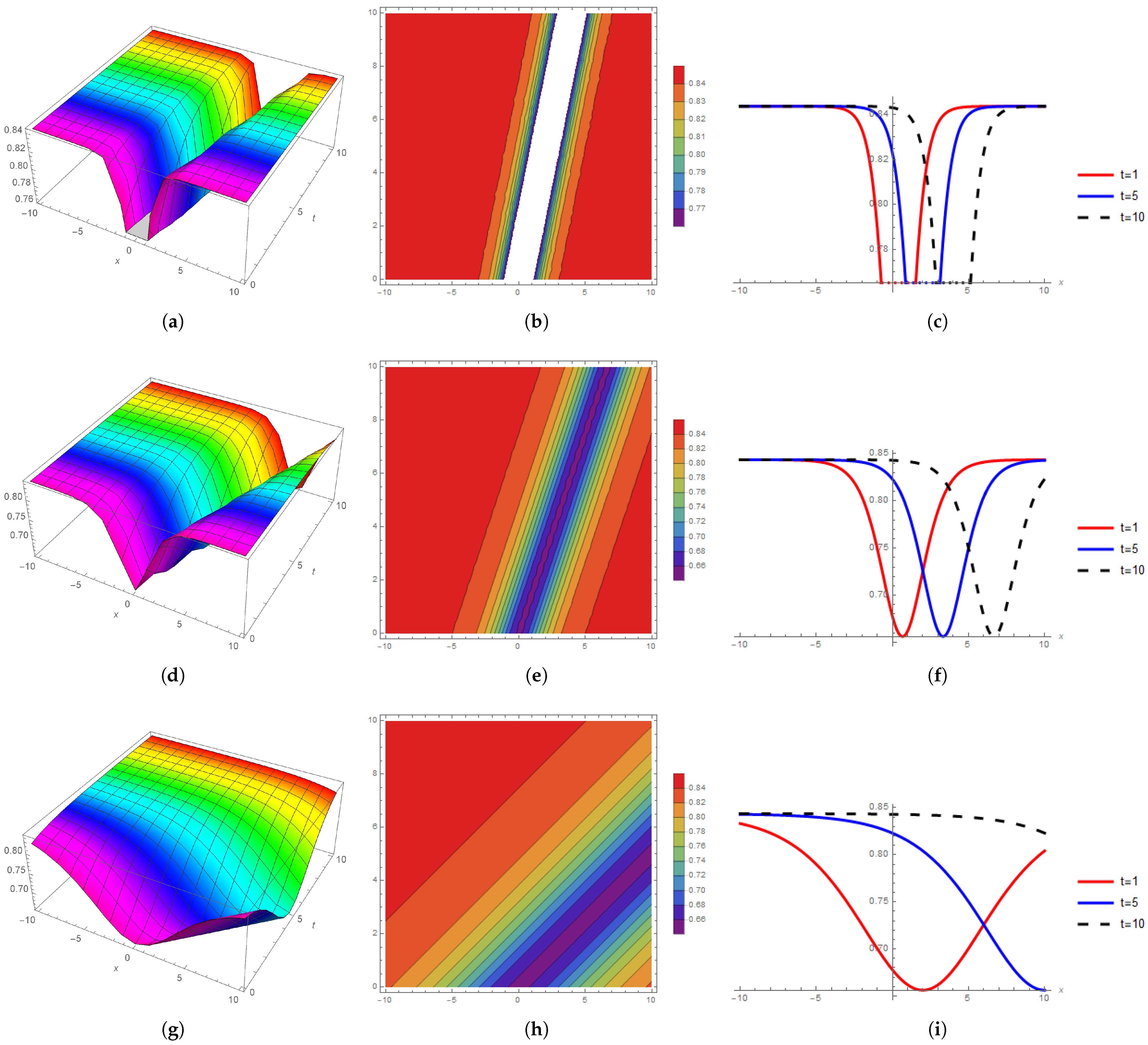
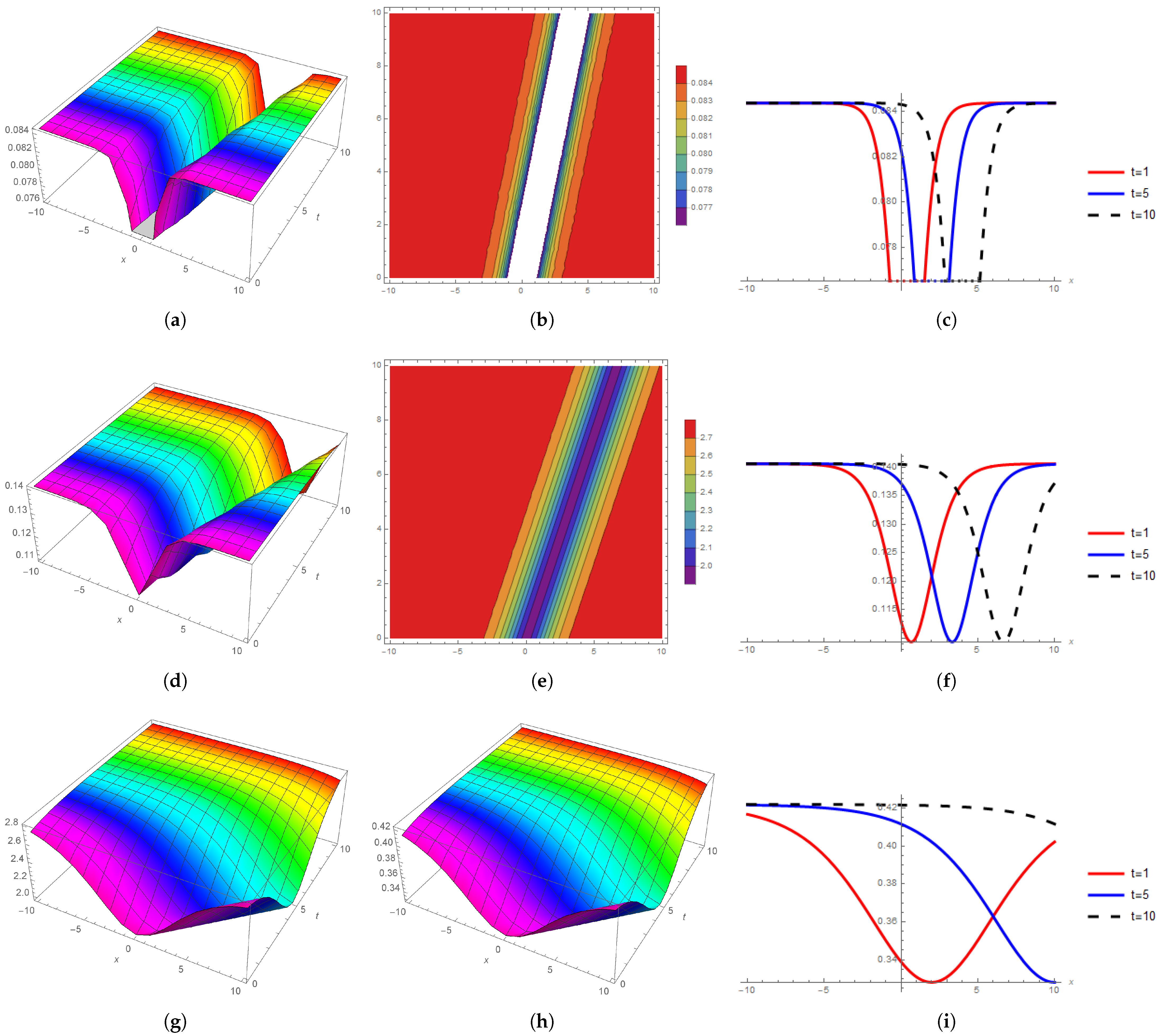
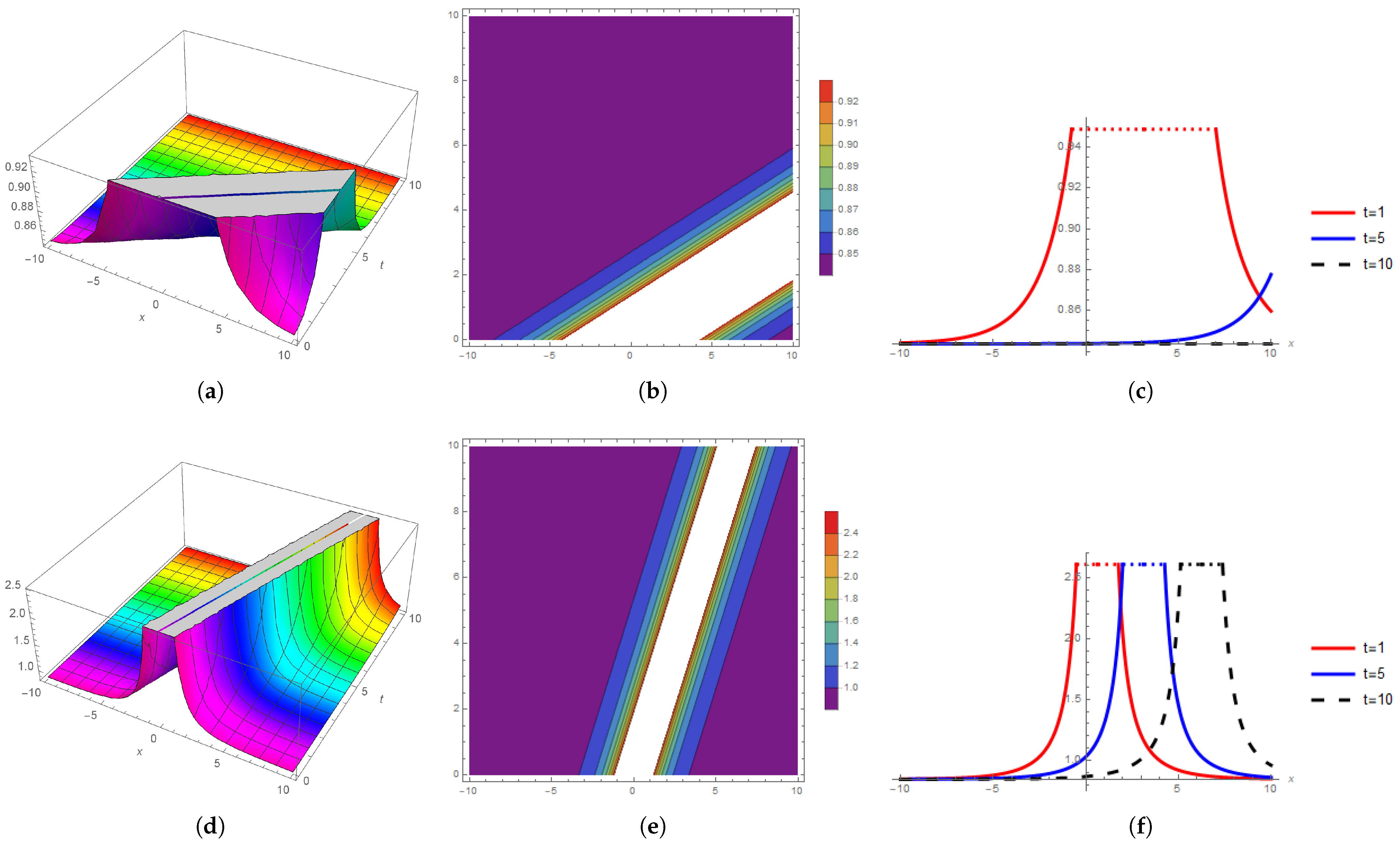
3. Graphical Representation

Graphical Discussion

In this part, we show 3D, contour, and 2D graphs of the calculated solutions to the soliton velocity and wave number under consideration. The wave solution was used to generate various sorts of graphs. The form of the traveling wave varies (as the unknown factors associated with the solution changed when we investigated the nature of the solution). The graphs representing the solutions to the succeeding nonlinear evolution equations of the Riemann wave equation are now shown. A current modern programming software application is used to plot the graph for better presentation, corresponding numerical values for parameters can be used based on their physical ranges.

In Figure 1 and Figure 2, we explained the graphical representation of the obtained solutions for soliton velocity at the parametric values $\beta =1.5$, $\alpha =1$, $\gamma =1$, $b_0=1.5$, $\mathfrak{S}=0.5$, $\lambda =0.8$, $\omega =0.25$, and Figure 1 depicts the solution’s nonlinear propagation behavior of ${\mathcal{U}}_1\left(\xi \right)$. At $c=2.5$, Figure 1a shows the kink 3D soliton by the Riemann wave equation, Figure 1b shows the singular contour soliton, and Figure 1c shows the bright 2D behavior. At $c=1.5$; Figure 1d shows the kink 3D shape soliton by the Riemann wave equation, Figure 1e shows the singular contour soliton and Figure 1f shows the bright 2D behavior. At $c=0.5$, Figure 1g shows the anti-bell kink shape 3D soliton; Figure 1h shows the singular contour soliton, and Figure 1i shows the bright periodic 2D behavior.

Figure 2 depicts the solution’s nonlinear propagation behavior of ${\mathcal{V}}_1\left(\xi \right)$. At $c=2.5$, Figure 2a shows the kink shape 3D soliton by the Riemann wave equation, Figure 2b shows the singular contour soliton and Figure 2c shows the bright 2D behavior. At $c=1.5$, Figure 2d shows the flat kink anti-bell shape 3D soliton by the Riemann wave equation, Figure 2e shows the singular contour soliton, and Figure 2f shows the bright 2D behavior. At $c=0.5$, Figure 2g strict anti-bell kink shape 3D soliton Figure 2h shows the singular contour soliton and Figure 2i shows the bright periodic 2D behavior.

In Figure 3 and Figure 4 we explain the graphical representation of the obtained solutions for the wave number at the parametric values $\beta =1.5$, $\alpha =1$, $\gamma =1$, $b_0=1.5$, $\mathfrak{S}=0.5$, $c=1$, $\omega =0.25$, Figure 3 depicts the solution’s nonlinear propagation behavior of ${\mathcal{U}}_1\left(\xi \right)$. At $\lambda =2.5$, Figure 3a shows the anti-bell shape 3D soliton by the Riemann wave equation, Figure 3b shows the singular contour soliton and Figure 3c shows the bright 2D behavior. At $\lambda =1.5$, Figure 3d shows the anti-bell kink shape 3D soliton by the Riemann wave equation, Figure 3e shows the singular contour soliton, and Figure 1f shows the bright 2D behavior. At $\lambda =0.5$, Figure 3g’s flat kink 3D soliton Figure 3h shows the singular contour soliton and Figure 1i shows the bright periodic 2D behavior.

Figure 4 depicts the solution’s nonlinear propagation behavior of ${\mathcal{V}}_1\left(\xi \right)$. At $\lambda =2.5$, Figure 4a shows the kink anti-bell 3D soliton by the Riemann wave equation, Figure 4b shows the singular contour soliton, and Figure 4c shows the bright 2D behavior. At $\lambda =1.5$, Figure 4d shows the anti-bell shape 3D soliton by the Riemann wave equation, Figure 4e shows the singular contour soliton, and Figure 4f shows the bright 2D behavior. At $\lambda =0.5$, Figure 4g’s strict flat kink shape 3D soliton Figure 4h shows the singular contour soliton and Figure 4i shows the bright periodic 2D behavior.

Figure 5 depicts the solution’s nonlinear propagation behavior of ${\mathcal{U}}_7\left(\xi \right)$, at the parametric values $\beta =1.5$, $\alpha =1$, $\gamma =1$, $b_0=1.5$, $\mathfrak{S}=0.5$, $\lambda =0.8$, $\omega =0.25$, at $c=2.5$, Figure 5a shows the bell shape kink 3D soliton by the Riemann wave equation, Figure 5b shows the singular contour soliton, and Figure 5c shows the bright 2D behavior. At $c=0.5$, the Figure 5d bell shape kink 3D soliton Figure 5e shows the singular contour soliton and Figure 5f shows the dark periodic 2D behavior.

Figure 6 shows the graphical representation of the nonlinear propagation behavior for the wave number at the parametric values $\beta =1.5$, $\alpha =1$, $\gamma =1$, $b_0=1.5$, $\mathfrak{S}=0.5$, and $c=1$, $\omega =0.25$; at $\lambda =2.5$, Figure 6a shows the bell kink shape 3D soliton by the Riemann wave equation, Figure 6b shows the singular contour soliton, and Figure 6c shows the bright 2D behavior. At $\lambda =0.5$, Figure 6d shows the bell shape kink 3D soliton, Figure 6e shows the singular contour soliton, and Figure 6f shows the bright periodic 2D behavior.

As a result, these physical descriptions of our novel results may be useful for nonlinear wave problems in applied sciences for further research.

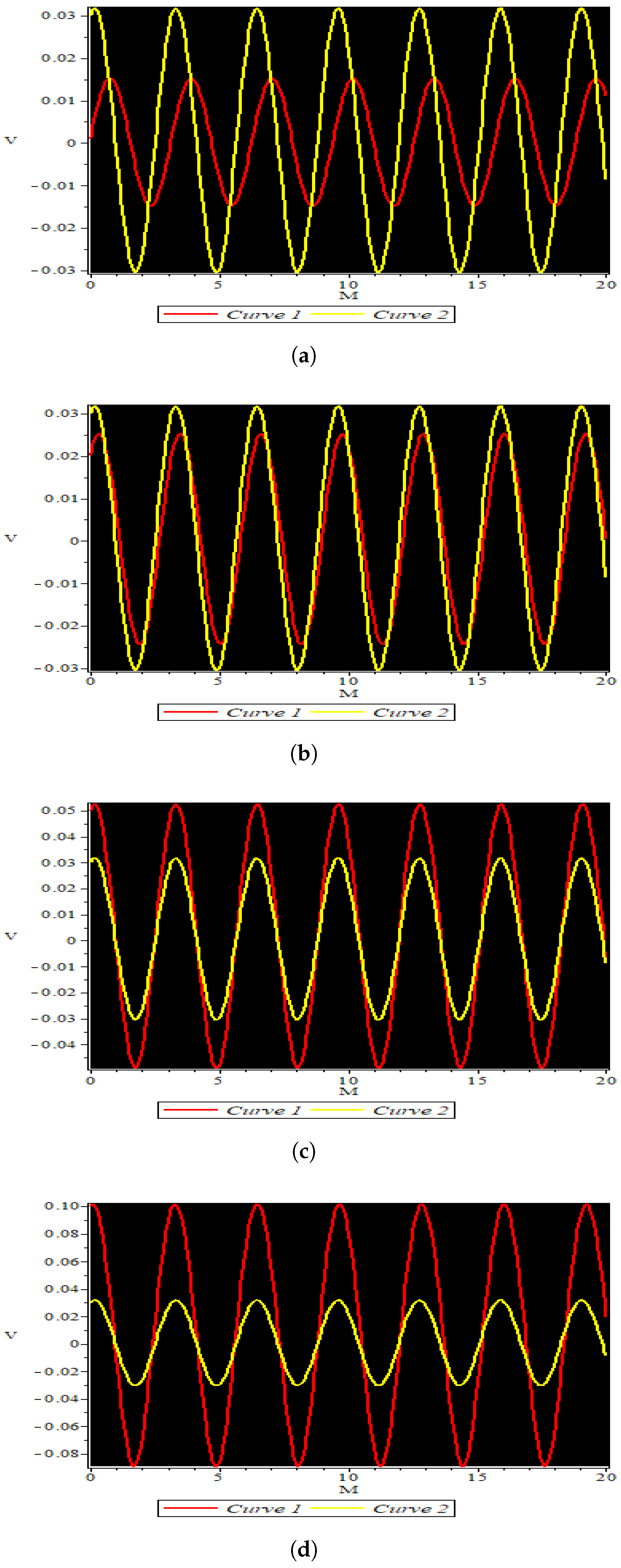
4. The Sensitivity Assessment

In order to display the sensitivity of the Riemann wave equation, the dynamic planer system can be contributed by using the Galilean transformation process. Thus, the Galilean transformation yields the dynamic system of Equation (46) as follows:

$$\begin{array}{c}\hfill \left\{\begin{array}{c}\frac{d\mathcal{U}}{d\xi }=S,\hfill \\ \frac{dS}{d\xi }=\frac{-(j+k){\mathcal{U}}^2}{2f{\lambda }^2}+\frac{c\mathcal{U}}{\omega f{\lambda }^2}.\hfill \end{array}\right.\end{array}$$

(119)

In Figure 7, we take parameters $c=1.2$, $j=1.5$, $k=0.9$, $\omega =2$, $f=0.6$, $\lambda =0.5$, where we investigate sensitive phenomena of the dynamical system given below,

The sensitivity analysis is a process that assesses how sensitive our system is. The system’s sensitivity will be poor if only a minor adjustment is made to the initial conditions. However, if the system suffers a considerable shift due to minor changes in the starting circumstances, the system will be extremely sensitive. As a result, the system is sensitive in this situation. Many figures are drawn for various initial conditions to highlight the system’s sensitivity. The changes in the amplitude and frequency of the wave velocity in the sensitivity graphs show the physical explanation for the system’s sensitivity.

5. Conclusions

This study investigated and examined the analytical solutions to the Riemann wave problem in a soliton theory. The explicit soliton structures were discussed using the new extended direct algebraic approach. As a result:

• We developed soliton solutions with twelve distinct families in which various newly different solutions were derived, such as the plane solution, mixed hyperbolic solution, trigonometry solution, mixed periodic and periodic solutions, shock solution, mixed singular solution, mixed trigonometric solution, mixed shock single solution, complex solitary shock solution, singular solution, and shock wave solutions.
• We displayed the 3D, 2D, and contour presentations of the obtained solutions with the appropriate values of involved parameters.
• A sensitivity analysis of the obtained system is displayed with the appropriate values of the involved parameters.
• The wave velocity and wave number parameters are responsible for controlling the singularity of the water waves.
• The new extended direct algebraic performance is reliable and effective, and it provides new solutions. The methodology utilized in this study will be used in future research to discover novel solutions for other nonlinear wave equations.

Researchers and professionals may apply these results to new nonlinear equations and complex nonlinear systems more quickly and efficiently.

References

1. Faridi, W.A.; Asjad, M.I.; Jarad, F. Non-linear soliton solutions of perturbed Chen-Lee-Liu model by Φ6-model expansion approach. Opt. Quantum Electron. 2022, 54, 664. [Google Scholar] [CrossRef]
2. Hosseini, K.; Mirzazadeh, M.; Salahshour, S.; Baleanu, D.; Zafar, A. Specific wave structures of a fifth-order nonlinear water wave equation. J. Ocean Eng. Sci. 2022, 7, 462–466. [Google Scholar] [CrossRef]
3. Aziz, N.; Seadawy, A.R.; Ali, K.; Sohail, M.; Rizvi, S.T.R. The nonlinear Schrödinger equation with polynomial law nonlinearity: Localized chirped optical and solitary wave solutions. Opt. Quantum Electron. 2022, 54, 458. [Google Scholar] [CrossRef]
4. Asjad, M.I.; Faridi, W.A.; Jhangeer, A.; Abu-Zinadah, H.; Ahmad, H. The fractional comparative study of the non-linear directional couplers in non-linear optics. Results Phys. 2021, 27, 104459. [Google Scholar]
5. Nisar, K.S.; Ciancio, A.; Ali, K.K.; Osman, M.S.; Cattani, C.; Baleanu, D.; Azeem, M. On beta-time fractional biological population model with abundant solitary wave structures. Alex. Eng. J. 2022, 61, 1996–2008. [Google Scholar]
6. Tariq, K.U.; Rezazadeh, H.; Zubair, M.; Osman, M.S.; Akinyemi, L. New Exact and Solitary Wave Solutions of Nonlinear Schamel–KdV Equation. Int. J. Appl. Comput. Math. 2022, 8, 114. [Google Scholar]
7. Pan, C.; Bu, L.; Chen, S.; Mihalache, D.; Grelu, P.; Baronio, F. Omnipresent coexistence of rogue waves in a nonlinear two-wave interference system and its explanation by modulation instability. Phys. Rev. Res. 2021, 3, 033152. [Google Scholar]
8. Bu, L.; Baronio, F.; Chen, S.; Trillo, S. Quadratic Peregrine solitons resonantly radiating without higher-order dispersion. Opt. Lett. 2022, 47, 2370–2373. [Google Scholar] [CrossRef] [PubMed]
9. Li, Z.; Xie, X.; Jin, C. Phase portraits and optical soliton solutions of coupled nonlinear Maccari systems describing the motion of solitary waves in fluid flow. Results Phys. 2022, 41, 105932. [Google Scholar] [CrossRef]
10. Shen, Y.; Tian, B.; Gao, X.T. Bilinear auto-Bäcklund transformation, soliton and periodic-wave solutions for a (2+1)-dimensional generalized Kadomtsev–Petviashvili system in fluid mechanics and plasma physics. Chin. J. Phys. 2022, 77, 2698–2706. [Google Scholar]
11. Faridi, W.A.; Asjad, M.I.; Jhangeer, A. The fractional analysis of fusion and fission process in plasma physics. Phys. Scr. 2021, 96, 104008. [Google Scholar] [CrossRef]
12. Faridi, W.A.; Asjad, M.I.; Eldin, S.M. Exact Fractional Solution by Nucci’s Reduction Approach and New Analytical Propagating Optical Soliton Structures in Fiber-Optics. Fractal Fract. 2022, 6, 654. [Google Scholar] [CrossRef]
13. Akinyemi, L.; Şenol, M.; Huseen, S.N. Modified homotopy methods for generalized fractional perturbed Zakharov–Kuznetsov equation in dusty plasma. Adv. Differ. Equ. 2021, 2021, 45. [Google Scholar] [CrossRef]
14. Ali, K.K.; Cattani, C.; Gómez-Aguilar, J.F.; Baleanu, D.; Osman, M.S. Analytical and numerical study of the DNA dynamics arising in oscillator-chain of Peyrard-Bishop model. Chaos Solitons Fractals 2020, 139, 110089. [Google Scholar] [CrossRef]
15. Aktar, M.S.; Akbar, M.A.; Osman, M.S. Spatio-temporal dynamic solitary wave solutions and diffusion effects to the nonlinear diffusive predator-prey system and the diffusion-reaction equations. Chaos Solitons Fractals 2022, 160, 112212. [Google Scholar] [CrossRef]
16. Bruzzone, O.A.; Perri, D.V.; Easdale, M.H. Vegetation responses to variations in climate: A combined ordinary differential equation and sequential Monte Carlo estimation approach. Ecol. Inform. 2022, 73, 101913. [Google Scholar] [CrossRef]
17. Zhou, T.Y.; Tian, B.; Zhang, C.R.; Liu, S.H. Auto-Bäcklund transformations, bilinear forms, multiple-soliton, quasi-soliton and hybrid solutions of a (3+1)-dimensional modified Korteweg-de Vries-Zakharov-Kuznetsov equation in an electron-positron plasma. Eur. Phys. J. Plus 2022, 137, 912. [Google Scholar] [CrossRef]
18. Poguluri, S.K.; Kim, J.; George, A.; Cho, I.H. Wave interaction with horizontal multilayer porous plates. J. Waterw. Port Coast. Ocean. Eng. 2022, 148, 04022016. [Google Scholar] [CrossRef]
19. Alabedalhadi, M. Exact traveling wave solutions for nonlinear system of spatiotemporal fractional quantum mechanics equations. Alex. Eng. J. 2022, 61, 1033–1044. [Google Scholar] [CrossRef]
20. Akinyemi, L.; Rezazadeh, H.; Yao, S.W.; Akbar, M.A.; Khater, M.M.; Jhangeer, A.; Ahmad, H. Nonlinear dispersion in parabolic law medium and its optical solitons. Results Phys. 2021, 26, 104411. [Google Scholar] [CrossRef]
21. Akinyemi, L.; Şenol, M.; Rezazadeh, H.; Ahmad, H.; Wang, H. Abundant optical soliton solutions for an integrable (2+1)-dimensional nonlinear conformable Schrödinger system. Results Phys. 2021, 25, 104177. [Google Scholar] [CrossRef]
22. Fahim, M.R.A.; Kundu, P.R.; Islam, M.E.; Akbar, M.A.; Osman, M.S. Wave profile analysis of a couple of (3+1)-dimensional nonlinear evolution equations by sine-Gordon expansion approach. J. Ocean Eng. Sci. 2022, 7, 272–279. [Google Scholar] [CrossRef]
23. Ozdemir, N.; Esen, H.; Secer, A.; Bayram, M.; Sulaiman, T.A.; Yusuf, A.; Aydin, H. Optical solitons and other solutions to the Radhakrishnan-Kundu-Lakshmanan equation. Optik 2021, 242, 167363. [Google Scholar] [CrossRef]
24. Osman, M.S.; Almusawa, H.; Tariq, K.U.; Anwar, S.; Kumar, S.; Younis, M.; Ma, W.X. On global behavior for complex soliton solutions of the perturbed nonlinear Schrödinger equation in nonlinear optical fibers. J. Ocean Eng. Sci. 2022, 7, 431–443. [Google Scholar] [CrossRef]
25. Kumar, S.; Dhiman, S.K.; Baleanu, D.; Osman, M.S.; Wazwaz, A.M. Lie symmetries, closed-form solutions, and various dynamical profiles of solitons for the variable coefficient (2+1)-dimensional KP equations. Symmetry 2022, 14, 597. [Google Scholar] [CrossRef]
26. Mirzazadeh, M.; Akinyemi, L.; Şenol, M.; Hosseini, K. A variety of solitons to the sixth-order dispersive (3+1)-dimensional nonlinear time-fractional Schrödinger equation with cubic-quintic-septic nonlinearities. Optik 2021, 241, 166318. [Google Scholar] [CrossRef]
27. Leventoux, Y.; Fabert, M.; Săpânţan, M.; Krupa, K.; Tonello, A.; Granger, G.; Couderc, V. Latest experimental advances in nonlinear multimode fiber optics. In Proceedings of the 2021 Conference on Lasers and Electro-Optics Europe & European Quantum Electronics Conference (CLEO/Europe-EQEC), Munich, Germany, 21–25 June 2021; p. 1. [Google Scholar]
28. Zafar, A.; Shakeel, M.; Ali, A.; Akinyemi, L.; Rezazadeh, H. Optical solitons of nonlinear complex Ginzburg–Landau equation via two modified expansion schemes. Opt. Quantum Electron. 2022, 54, 1–15. [Google Scholar]
29. Ali, K.K.; Wazwaz, A.M.; Osman, M.S. Optical soliton solutions to the generalized nonautonomous nonlinear Schrödinger equations in optical fibers via the sine-Gordon expansion method. Optik 2020, 208, 164132. [Google Scholar] [CrossRef]
30. Zhang, R.; Bilige, S.; Chaolu, T. Fractal solitons, arbitrary function solutions, exact periodic wave and breathers for a nonlinear partial differential equation by using bilinear neural network method. J. Syst. Sci. Complex 2021, 34, 122–139. [Google Scholar] [CrossRef]
31. Khater, M.; Jhangeer, A.; Rezazadeh, H.; Akinyemi, L.; Akbar, M.A.; Inc, M.; Ahmad, H. New kinds of analytical solitary wave solutions for ionic currents on microtubules equation via two different techniques. Opt. Quantum Electron. 2021, 53, 609. [Google Scholar] [CrossRef]
32. Karaman, B. The use of improved-F expansion method for the time-fractional Benjamin–Ono equation. Rev. Real Acad. Cienc. Exactas Fis. Nat. Ser. Mat. 2021, 115, 128. [Google Scholar] [CrossRef]
33. Zayed, E.M.; Gepreel, K.A.; Shohib, R.M.; Alngar, M.E.; Yıldırım, Y. Optical solitons for the perturbed Biswas-Milovic equation with Kudryashov’s law of refractive index by the unified auxiliary equation method. Optik 2021, 230, 166286. [Google Scholar] [CrossRef]
34. Ismael, H.F.; Bulut, H.; Baskonus, H.M. Optical soliton solutions to the Fokas–Lenells equation via sine-Gordon expansion method and (m+(G/G))(m+(G/G))-expansion method. Pramana 2020, 94, 35. [Google Scholar] [CrossRef]
35. Sulaiman, A.T.; Yusuf, A. Dynamics of lump-periodic and breather waves solutions with variable coefficients in liquid with gas bubbles. Waves Random Complex Media 2021, 6, 1–14. [Google Scholar] [CrossRef]
36. Khodadad, F.S.; Mirhosseini-Alizamini, S.M.; Günay, B.; Akinyemi, L.; Rezazadeh, H.; Inc, M. Abundant optical solitons to the Sasa-Satsuma higher-order nonlinear Schrödinger equation. Opt. Quantum Electron. 2021, 53, 702. [Google Scholar] [CrossRef]
37. Kumar, S.; Kumar, A.; Wazwaz, A.M. New exact solitary wave solutions of the strain wave equation in microstructured solids via the generalized exponential rational function method. Eur. Phys. J. Plus 2020, 135, 870. [Google Scholar] [CrossRef]
38. Wazwaz, A.M. Optical bright and dark soliton solutions for coupled nonlinear Schrödinger (CNLS) equations by the variational iteration method. Optik 2020, 207, 164457. [Google Scholar] [CrossRef]
39. Ghanbari, B.; Kumar, S.; Niwas, M.; Baleanu, D. The Lie symmetry analysis and exact Jacobi elliptic solutions for the Kawahara–KdV type equations. Results Phys. 2021, 23, 104006. [Google Scholar] [CrossRef]
40. Rehman, S.U.; Yusuf, A.; Bilal, M.; Younas, U.; Younis, M.; Sulaiman, T.A. Application of (GG-2)-expansion method to microstructured solids, magneto-electro-elastic circular rod and (2+1)-dimensional nonlinear electrical lines. Math. Eng. Sci. Aerosp. 2020, 11, 789–803. [Google Scholar]
41. Rashed, A.S.; Mabrouk, S.M.; Wazwaz, A.M. Forward scattering for non-linear wave propagation in (3+1)-dimensional Jimbo-Miwa equation using singular manifold and group transformation methods. Waves Random Complex Media 2022, 32, 663–675. [Google Scholar] [CrossRef]
42. Kumar, S.; Rani, S. Symmetries of optimal system, various closed-form solutions, and propagation of different wave profiles for the Boussinesq–Burgers system in ocean waves. Phys. Fluids 2022, 34, 037109. [Google Scholar] [CrossRef]
43. Abdulwahhab, M.A. Hamiltonian structure, optimal classification, optimal solutions and conservation laws of the classical Boussinesq–Burgers system. Part. Differ. Equ. Appl. Math. 2022, 6, 100442. [Google Scholar] [CrossRef]
44. Kumar, S.; Niwas, M.; Osman, M.S.; Abdou, M.A. Abundant different types of exact soliton solution to the (4+1)-dimensional Fokas and (2+1)-dimensional breaking soliton equations. Commun. Theor. Phys. 2021, 73, 105007. [Google Scholar] [CrossRef]
45. Abdulwahhab, M.A. On the invariant solutions, third order multipliers and local conservation laws of the 3-dimensional Pavlov Equation. Optik 2022, 168852. [Google Scholar] [CrossRef]
46. Pan, C.; Bu, L.; Chen, S.; Yang, W.X.; Mihalache, D.; Grelu, P.; Baronio, F. General rogue wave solutions under SU (2) transformation in the vector Chen–Lee–Liu nonlinear Schrödinger equation. Phys. D Nonlinear Phenom. 2022, 434, 133204. [Google Scholar] [CrossRef]
47. Shakeel, M.; Ahmad, B.; Shah, N.A.; Chung, J.D. Solitons Solution of Riemann Wave Equation via Modified Exp Function Method. Symmetry 2022, 14, 2574. [Google Scholar]
48. Spatschek, K.H.; Shukla, P.K. Nonlinear interaction of magneto-sound wave with whistler turbulence. Radio Sci. 1978, 13, 211–214. [Google Scholar] [CrossRef]
49. Islam, M.E.; Akbar, M.A. Stable wave solutions to the Landau-Ginzburg-Higgs equation and the modified equal width wave equation using the IBSEF method. Arab. J. Basic Appl. Sci. 2020, 27, 270–278. [Google Scholar] [CrossRef]
50. Barman, H.K.; Akbar, M.A.; Osman, M.S.; Nisar, K.S.; Zakarya, M.; Abdel-Aty, A.H.; Eleuch, H. Solutions to the Konopelchenko-Dubrovsky equation and the Landau-Ginzburg-Higgs equation via the generalized Kudryashov technique. Results Phys. 2021, 24, 104092. [Google Scholar] [CrossRef]
51. Kundu, P.R.; Almusawa, H.; Fahim, M.R.A.; Islam, M.E.; Akbar, M.A.; Osman, M.S. Linear and nonlinear effects analysis on wave profiles in optics and quantum physics. Results Phys. 2021, 23, 103995. [Google Scholar] [CrossRef]
52. Jhangeer, A.; Faridi, W.A.; Asjad, M.I.; Akgül, A. Analytical study of soliton solutions for an improved perturbed Schrödinger equation with Kerr law non-linearity in non-linear optics by an expansion algorithm. Part. Differ. Equ. Appl. Math. 2021, 4, 100102. [Google Scholar] [CrossRef]
53. Barman, H.K.; Seadawy, A.R.; Akbar, M.A.; Baleanu, D. Competent closed form soliton solutions to the Riemann wave equation and the Novikov-Veselov equation. Results Phys. 2020, 17, 103131. [Google Scholar] [CrossRef]
54. Seadawy, A.R.; Rizvi, S.T.R.; Ahmad, S.; Younis, M.; Baleanu, D. Lump, lump-one stripe, multiwave and breather solutions for the Hunter–Saxton equation. Open Phys. 2021, 19, 1–10. [Google Scholar] [CrossRef]
55. Hosseini, K.; Osman, M.S.; Mirzazadeh, M.; Rabiei, F. Investigation of different wave structures to the generalized third-order nonlinear Scrödinger equation. Optik 2020, 206, 164259. [Google Scholar] [CrossRef]
56. Rizvi, S.T.R.; Seadawy, A.R.; Ashraf, F.; Younis, M.; Iqbal, H.; Baleanu, D. Lump and interaction solutions of a geophysical Korteweg–de Vries equation. Results Phys. 2020, 19, 103661. [Google Scholar] [CrossRef]
57. Sulaiman, T.A.; Yusuf, A.; Alquran, M. Dynamics of optical solitons and nonautonomous complex wave solutions to the nonlinear Schrodinger equation with variable coefficients. Nonlinear Dyn. 2021, 104, 639–648. [Google Scholar] [CrossRef]
Figure 1. The 3D, contour, and 2D behavior comparisons for U 1 ( ξ ) ; (a) 3D wave profile at soliton velocity c = 2.5 ; (b) contour wave profile at soliton velocity c = 2.5 ; (c) 2D wave profile at soliton velocity c = 2.5 ; (d) 3D wave profile at soliton velocity at c = 1.5 ; (e) contour wave profile at soliton velocity c = 1.5 ; (f) 2D wave profile at soliton velocity c = 1.5 ; (g) 3D wave profile at soliton velocity c = 0.5 ; (h) contour wave profile at soliton velocity c = 0.5 ; (i) 2D wave profile at soliton velocity c = 0.5 .
Fractalfract 07 00102 g001
Figure 2. The 3D, contour, and 2D behavior comparison for V 1 ( ξ ) ; (a) 3D wave profile at soliton velocity c = 2.5 ; (b) contour wave profile at soliton velocity c = 2.5 ; (c) 2D wave profile at soliton velocity c = 2.5 ; (d) 3D wave profile at soliton velocity c = 1.5 ; (e) contour wave profile at soliton velocity c = 1.5 ; (f) 2D wave profile at soliton velocity c = 1.5 ; (g) 3D wave profile at soliton velocity c = 0.5 ; (h) contour wave profile at soliton velocity c = 0.5 ; (i) 2D wave profile at soliton velocity c = 0.5 .
Fractalfract 07 00102 g002
Figure 3. The 3D, contour, and 2D behavior comparison for U 1 ( ξ ) ; (a) 3D wave profile at wave number λ = 2.5 ; (b) contour wave profile at wave number λ = 2.5 ; (c) 2D wave profile at wave number λ = 2.5 ; (d) 3D wave profile at wave number λ = 1.5 ; (e) contour wave number soliton solution at λ = 1.5 ; (f) 2D wave profile at wave number λ = 1.5 ; (g) 3D wave profile at wave number λ = 0.5 ; (h) contour wave profile at wave number λ = 0.5 ; (i) 2D wave profile at wave number λ = 0.5 .
Fractalfract 07 00102 g003
Figure 4. The 3D, contour, and 2D behavior comparison for V 1 ( ξ ) ; (a) 3D wave profile at wave number λ = 2.5 ; (b) contour wave profile at wave number λ = 2.5 ; (c) 2D wave profile at wave number λ = 2.5 ; (d) 3D wave profile at wave number λ = 1.5 ; (e) contour wave profile at wave number λ = 1.5 ; (f) 2D wave profile at wave number λ = 1.5 ; (g) 3D wave profile at wave number λ = 0.5 ; (h) contour wave profile at wave number λ = 0.5 ; (i) 2D wave profile at wave number λ = 0.5 .
Fractalfract 07 00102 g004
Figure 5. The 3D, contour, and 2D behavior comparison for U 7 ( ξ ) ; (a) 3D wave profile at soliton velocity c = 2.5 ; (b) contour wave profile at soliton velocity c = 2.5 ; (c) 2D wave profile at soliton velocity c = 2.5 ; (d) 3D wave profile at soliton velocity c = 0.5 ; (e) contour wave profile at soliton velocity c = 0.5 ; (f) 2D wave profile at soliton velocity c = 0.5 .
Fractalfract 07 00102 g005
Figure 6. The 3D, contour, and 2D behavior comparison for U 7 ( ξ ) ; (a) 3D wave profile at wave number λ = 2.5 ; (b) contour wave profile at wave number λ = 2.5 ; (c) 2D wave profile at wave number λ = 2.5 ; (d) 3D wave profile at wave number λ = 0.5 ; (e) contour wave profile at wave number λ = 0.5 ; (f) 2D wave profile at wave number λ = 0.5 .
Fractalfract 07 00102 g006
Figure 7. Sensitivity assessment at different initial conditions. (a) Sensitive visualization for curve 1 at (0.001, 0.03) and curve 2 at (0.03, 0.02); (b) sensitive visualization for curve 1 at (0.02, 0.03) and curve 2 at (0.03, 0.02); (c) sensitive visualization for curve 1 at (0.05, 0.03) and curve 2 at (0.03, 0.02); (d) sensitive visualization for curve 1 at (0.1, 0.03) and curve 2 at (0.03, 0.02).
Fractalfract 07 00102 g007
Disclaimer/Publisher’s Note: The statements, opinions and data contained in all publications are solely those of the individual author(s) and contributor(s) and not of MDPI and/or the editor(s). MDPI and/or the editor(s) disclaim responsibility for any injury to people or property resulting from any ideas, methods, instructions or products referred to in the content.