Abstract
This paper presents a detailed investigation of a stochastic model that rules the spreading behavior of the measles virus while accounting for the white noises and the influence of immunizations. It is hypothesized that the perturbations of the model are nonlinear, and that a person may lose the resistance after vaccination, implying that vaccination might create temporary protection against the disease. Initially, the deterministic model is formulated, and then it has been expanded to a stochastic system, and it is well-founded that the stochastic model is both theoretically and practically viable by demonstrating that the model has a global solution, which is positive and stochastically confined. Next, we infer adequate criteria for the disease’s elimination and permanence. Furthermore, the presence of a stationary distribution is examined by developing an appropriate Lyapunov function, wherein we noticed that the disease will persist for and that the illness will vanish from the community when . We tested the model against the accessible data of measles in Pakistan during the first ten months of 2019, using the conventional curve fitting methods and the values of the parameters were calculated accordingly. The values obtained were employed in running the model, and the conceptual findings of the research were evaluated by simulations and conclusions were made. Simulations imply that, in order to fully understand the dynamic behavior of measles epidemic, time-delay must be included in such analyses, and that advancements in every vaccine campaign are inevitable for the control of the disease.
1. Introduction
Measles is still a major worldwide health issue, particularly in the less developed countries. Measles (also known as Rubella or morbilli) is an extremely contagious illness caused mostly by the Morbillivirus genus in the Paramyxovirus [1,2]. Although efficient vaccines against this severe illness are commonly accessible, still measles is a leading cause of death among children below five of years of age [3]. The disease infecting hundreds of millions of children each year and resulting in a high mortality and morbidity in the child population, owing primarily to complicated conditions that exist side by side with the disease like malnutrition, diarrhea, and pneumonia [4]. Sneezing and coughing, touching the nasal or aerosol fluids, or close physical touch with an infected person are all ways to spread measles. It can stay extremely contagious for a maximum of two hours in the atmosphere and on the surfaces. Clinical manifestations include soar throat, cough, nasal congestion, blurred vision, and small white patches in the mouth; these signs and symptoms often develop within 10–12 days post-infection. Subsequently, a rash appears, extending downward out of the nose. The period of peak infectivity (virus shed) starts four days before that and four days just after commencement of the rashes. The usual incubation time is 14 days; however, it can range from 7–18 days [5]. In reality, even vaccinated people may still be susceptible if the immunization fails or existing immunity from the vaccine wears off. Despite the fact that vaccination has cut worldwide measles fatalities by 73% between 2000–2018, measles continues to remain a widespread in many underdeveloped nations, particularly in Asia and Africa. Around 140,000 individuals died from the measles in 2018. During 2000–2018, worldwide measles immunization results in an 85 percent drop in measles transmission [6,7]. Despite the abundance of a safe and effective vaccination in 2017, around 110,000 deaths occurred from measles, primarily children under the age of six, as per the report of the World Health Organization (WHO) [8]. Vaccination is amongst the most successful health promotion strategy for reducing death rates and the spreading of epidemics; it has been demonstrated that vaccination saves over 3 million people only in Nigeria every year. The vaccination will work with the immune system of the body to establish the body’s natural defenses, reducing the likelihood of relapse [9]. The MMR vaccination can protect against measles, which is a vaccine-preventable illness. The MMR vaccines are highly effective at protecting both adults and children from the epidemic measles. Only one dose of the MMR vaccines is roughly 92% successful in suppressing the measles, whereas two doses are around 95% effective. The MMR vaccine also protects against rubella and mumps [10]. This disease is an endemic one in Nigeria, with epidemics occurring at regular intervals. Measles is present across Nigeria at all seasons; however, it is more widespread in the summer months.
Pakistan is one of the most measles-affected nations in Asia [11]. Every 8–10 years, the nation has a recurring measles epidemic. In fact, 2845 identified measles infections were reported in Pakistan during the year 2016. This figure increased to 6791 in 2017 and, in the year 2018, 33,007 cases were reported. These results represent about 44, 20, and 51 percent of the total number of cases recorded in the East Mediterranean, which includes 22 nations. In 2017, over 130 children lost their lives due to this infection, with the figure rising to nearly 300 in 2018 [12].
It is strongly advised to employ the methods of mathematical modeling to examine the transmission process and prevention of an epidemic disease [7,13,14,15], modeling with fractional differential equations also have several applications in all fields of science [16,17,18]. While depicting the natural history of an infectious disease, the tools of modeling can create a balance among the data and its real biology. Thus far, models responsible for describing the dynamics of measles both from population to outbreak levels have demonstrated a wide variety of disease patterns. External noise is usually the main significant feature of physical processes and bio-systems. It has been discovered that environmental variables have a significant impact on the dynamics of measles disease spread [19]. Because of the uncertainty of person-to-person interactions or inherent characteristics of the population, outbreak onset and propagation are fundamentally unpredictable. As a result, the condition of the disease is influenced by the environment’s heterogeneity and uncertainty.
Changes in the environment likewise have a significant impact on the parasites’ persistence and distribution. Because the stochasticity of parameters and states depicts the exact dynamic behavior of an infectious disease, it is regarded as an essential part in epidemiological studies. Even though the perturbations are varying, these should be autocorrelated in a positive way. Furthermore, the perturbations may be estimated theoretically using the linked problem’s probability density function [20,21,22,23]. There are two main techniques to epidemic modeling: the deterministic modeling and stochastic modeling. Stochastic differential equation (SDE) models are recommended over deterministic models for mathematical modeling of biological functions because they may provide a higher level of reality than their deterministic equivalents [23,24,25,26]. We may choose to use SDEs to generate a distribution of the predicted output(s); for example, the number of infected individuals over time t. Moreover, when tested numerous times, a stochastic model produces more useful outputs than a deterministic one. A deterministic model, on the other hand, will produce only one outcome irrespective of the number of experiments. To explain the viral evolution of COVID-19, numerous deterministic infectious disease models have been suggested; for example, see [27,28].
The rest of the manuscript is organized in the following manner: Section 2 deals with the formulation of the proposed stochastic model for the spreading of the epidemic measles. The uniqueness and existence problem for obtaining a positive global solution is presented in Section 3. In Section 4 and Section 5, we characterized sufficient criteria for the stationary distribution and extinction of the disease. We optimize the proposed model using data from Pakistan compiled in the first ten months of 2019 in Section 6. We quantitatively compared the obtained analytical results, and graphical illustrations were presented in Section 7. We concluded the work in Section 8 by presenting the future directions and a comprehensive summary.
2. Model Formulation
Olumuyiwa et al. [29] have recently developed a model of the transmission of rubella disease by using the differential equations. Keeping in view the work of Olumuyiwa et al., here we intend to extend the model to a stochastic model. Furthermore, by considering different stages during the measles epidemic, we stratified the total population into six disjoint classes, namely: susceptible, vaccinated, exposed, infectious, hospitalized and recovered individuals whose sizes in mathematical terms are, respectively, , and .
The entrance of new persons through this population is captured by the rate and will be kept in the susceptible compartment. People in the vulnerable group start receiving a vaccination at a rate and setback immune function at a vaccine wane rate . The contact rate of susceptible persons is , and thus the term force of infection becomes , with the transition again from exposures to infection stages occurring at a rate of . People who are infected with the measles seek medical attention at a rate of and recover from the infection after the successful treatment supplemented at a rate of . We consider two types of death rates: the natural (that is constant for all classes) and the disease-induced mortality rate . This study assumes the recovery from measles that is possible due to the treatment only, that is, the study considering no natural recovery. The movements between the compartments are depicted via a flowchart in Figure 1. The above assumptions will lead to the following deterministic system:
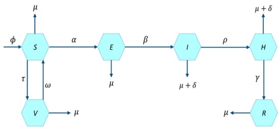
Figure 1.
Flow chart of the measles model (1) [29].
The threshold parameter has the following expression for model (1) as
In order to consider the noises due the environment in the study (i.e., model (1)), we shall take into account the standard Brownian motions for with . Furthermore, system (1) is modified by considering the incidence rate of bi-linear form . For the noise intensities, we have taken as the relative weights. By considering these stochastic terms, the deterministic model (1) takes the form
Keeping in view system (3), the authors have a keen interest to find the possible answers to the following questions:
- Q1:
- What role do the random noises play in the transmission measles?
- Q2:
- What role contaminated vaccination in the spreading of measles disease?
- Q3:
- Under what condition(s) will the disease tend to go extinct?
- Q4:
- Under what condition(s) will the epidemic measles persist in the population?
3. Stochastic Model Analysis
This section investigates the existence/uniqueness of solutions, global asymptotic behavior, derivation of conditions under which the disease tends to go extinct, and the presence of an ergodic stationary distribution for the proposed stochastic model.
Positive Global Solution of the Model
The very first crucial question in studying the dynamic behavior is whether there is a possibility of the existence of a global solution to the model. Furthermore, for a system modeling the population dynamics, the nature of the solution’s value is of major relevance. In addition, we demonstrate in this section that the solution of randomized system (3) is global in nature and positive. It is well established that, for every given initial amount, the coefficients of a stochastic equation must fulfill the normal growth constraint and the local Lipschitz criterion in order to have a unique global solution (i.e., without any explosion in a limited period).
Theorem 1.
There exists a unique solution of system (3) for under the initial conditions from the state . Moreover, the solution remains in the same space (i.e., ) surely for .
Proof.
Keeping in view the Lipschitzness of the coefficients used in the model and from the fact , we can say that the proposed system has a unique local solution in and . The term stands for the explosion time, and readers are referred to [30,31] for a detailed analysis. By showing that, actually , we reach the conclusion that such a solution is global in nature. To do so, it is necessary that we assume a large in such a way that contains all parts of the solution. Assume and let us define
Whenever represents the empty set, then we shall write . By increasing the value of k, one can notice that it increases . We apply the limit and assume that the and a.s. . Thus, if we show a.s., it ensures . Proving all these guarantees that for any time . Let us assume the contrary case that ; then, there must exist positive real numbers T and in such a way
Thus, for an integer , we have
To begin, first let us establish a Lyapunov function of the type
By utilizing the formula due to , letting and assuming a very large non-negative real T, Equation (6) can be written in the form of
In Equation (23), the operator is from the space to . □
The remaining parts of the proof are merely similar to Theorem 2.1 in [26,30]. Thus, it is very simple for the reader to follow the result and and hence, is not completely proved here.
4. Extinction
While modeling the dynamical aspects of any epidemic diseases, it is important to investigate the situations under which the disease will become exterminated or tend to become extinct in the community. Within this section, we demonstrate that, when the white noises are large enough, the solution of the associated stochastic model (3) surely vanishes. Let us define
Lemma 1.
(Strong Law)[32,33]Let be continuous and real valued along with a local martingale, which vanishes as , then
Lemma 2.
Assume that corresponds to initial data in the space and is a solution of model (3). Then,
Furthermore, if , and , then
Then, the solution of (3)
To prove Lemma 2, we follow almost the same techniques as performed in proving Lemmas 2.1 and 2.2 carried out in the work of Zhao [32], and thus the readers can simply prove the results.
Next, to develop the extinction theory related to model (3), we first define the threshold quantity for the proposed stochastic model which can be written in the form of
Theorem 2.
Proof.
Let correspond to initial data in the space , being a solution of model (3).
Define
Differentiating Equation (13) following Ito’s formula, one can obtain
By taking the integral of either sides of the above inequality over the interval , we have
By assuming the as and multiplying both sides of relation (15) by while considering Lemma 2, we obtain
If , then if . Again, and we assert that —hence the result. □
5. The Stationary Distribution of the Disease
We understand that there are no endemic states in stochastic models. As a result, the stability of the system cannot be used to predict how long an illness would endure. As a result, one must concentrate on the existence/uniqueness assumption of the stationary distribution. In certain aspects, this assists the illness with survival. For this purpose, we employ a well-known method due to Hasminskii [34].
Assume a homogeneously time-dependent Markov process in the space that satisfies the below stochastic model
The diffusion matrix can be demonstrated as:
Lemma 3.
for all
[34]. The process has a one and only one stationary distribution whenever there is a bounded domain having a regular boundary in such a way that closure and having the below characteristics
- The smallest eigenvalue of the matrix is bounded below from the origin in the open domain U and in its neighborhood.
- For the average time period τ (at which a path starts from ϰ reaching the set U) is bounded, and for every compact subset , we have . When is an integrable function with the measure , then we have
Let us define the following parameter for our future use:
Theorem 3.
For , then a solution of system (3) is ergodic and has one and only one stationary distribution .
Proof.
For verifying condition (2) of Lemma (3), we must develop a positive function To do so, we first formulate
where and are all real and positive constants, and must be calculated later on. By assuming the formula due to Itô’s and keeping in view system (3), we obtain
□
Hence,
The preceding calculation indicates that
Suppose
Namely,
As a result,
Furthermore, we obtain
where is an unknown real number and must be determined later. It is very helpful to state
where .
In the below steps, we show that actually the function has the minimum value, . The partial derivatives of the function with respect to the state variables are given by:
One can verify very easily that the function has only one stagnation point.
Furthermore, at for , the Hessian matrix is as follows:
The Hessian matrix is obviously positive definite. As a result, the minimum value of is . We may assert that has one and only one minimum value inside based on Equation (20) and the continuity of . Then, as follows, we delineate a non-negative function :
Using formula and the suggested system, we arrive at
Based on the above result, we have the following assertion:
where
Overall, for the solution to the model, we have the following set
where are extremely small positive real values to be calculated later on. For the sake of simplicity, the whole set was partitioned into the following subsets:
Then, we show that on , which is the same is displaying the solution on the eight sub-regions.
Case 1.
If , then, by Equation (24), we obtain
For every , picking returns .
Just as in the proof above, we conclude that for , .
As a result, we arrived to the point that there must be positive constant in such a way
Thus,
Consider , and is the amount of time it takes for a path to start from to achieve set D,
The next relation could be obtained if one integrates the above inequality from 0 to , considering the expectation and using Dynkin’s formula:
Hence, is non-negative; then,
We have as a result of the proof of Theorem (3). This also shows that model (3) is regular and, consequently, by letting , almost surely we have .
Moreover, by utilizing the Fatou’s lemma, we have
where K is the compact set, i.e., a subset of . This proves the condition (2) of Lemma (3) in an alternative approach.
Additionally, the diffusion matrix for the system (3) is
Taking we obtain
where Similarly, this proves condition (1) of Lemma (3). Keeping in view the previous statements, the ergodicity of model (3) is insured by Lemma (3) and hence proving that the model has stationary distribution.
6. Parameter Estimation
Among the most important processes to carry through out the testing process is the utilization of real data (if available) to acquire findings for certain unidentified biological factors used in the epidemiology system under study. Real-world measles cases, as shown in Table 1, are used to test the proposed rubella model and to choose the best fitted parameters for numerous unknown biological parameters that emerge in the system. Considering the 2018 statistics of WHO, the natural death rate of a Pakistani individual is since the life expectancy of a Pakistani is . In addition, the entire size of the country is , whereas the recruitment rate is calculated to be . Additionally, Memon et al. [13] indicates that the rate of measles vaccination is generally 97 percent effective, implying that the vaccines’ effectiveness equals . Some values of the parameters are estimated and others were fitted against the data, and these were presented in Table 2. In Figure 2, the results via simulations for measles resurgence cases obtained by adapting the proposed model (3) with real data from the first ten months of the year 2019 are shown. As shown in Figure 2, it gives a rather good match, lending veracity to the predictions generated from the proposed measles model (3). We employed the relation to measure the associated relative error for fitting the model against the data.

Table 1.
Real cases of the measles epidemic in Pakistan during January and October 2019.
Table 2.
Values of the parameters estimated and fitted against the real measles cases.
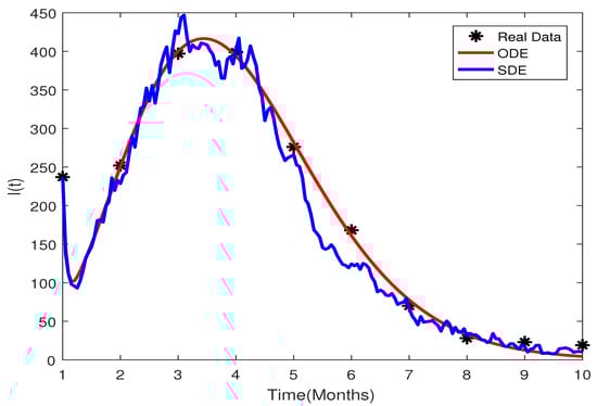
Figure 2.
The figure shows the fitting of both ODE and SDE models against the real data by using values of the parameters shown in Table 2.
7. Numerical Simulations and Discussion
It is of great concern to simulate each mathematical model against the real data and to verify theoretical results, and this step is very important when dealing with modeling biological problems. The researchers seek to simulate problem (3) employing classic numerical algorithms that rapidly converged. Almost all of the theoretical conclusions are quantitatively validated by using the well-known RK-4 approach.
where stands for the standard Gaussian stochastic variables, having distribution and is the constant time-step. The terms reflect the intensities of the white noises.
To quantitatively validate the analytical conclusions, we require the parameters’ value being used in model (3). In Example 1 and 2, we established two sets of parameters’ values for this reason, and the population levels of each compartment at were displayed. For every scenario, we simulated the model over the interval .
We formulated Theorem 2 based on the stochastic theory of stability, which indicates that, under the condition of , the infection would continue to perish from the community regardless of the levels of the variables at . Furthermore, the theory demonstrates that the infection will be eradicated from the community with unit probability. Figure 3 shows that the random curves reach the infection-free state after a limited period of time, confirming the analytical results.
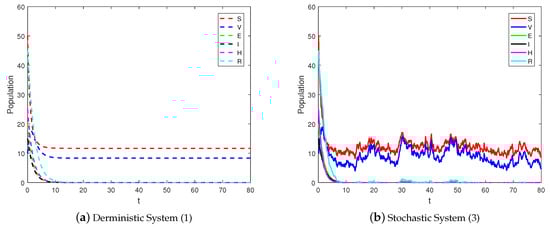
Figure 3.
Sample solutions of stochastic systems (3) with its associated deterministic counterpart.
Example 1.
The values of the parameter are assumed as: and , where the initial values of the state vector are . Similarly, the intensities of the white noises are: . Using those same model parameters, we estimated , which was found to be lower than 1. As a result, the assumption of Theorem 2 is met, and hence the components of the solution of the model adhere to the following relations:
Essentially, these relations explain the elimination of the virus from the community, as seen by Figure 3. As a consequence, the derived research findings on elimination are valid and may be relied on.
Likewise, Theorem 3 guarantees the disease’s prevalence in the population given permissible limits. By considering data from Example 2, we calculated the value of , and it was found that it is greater than unity. Figure 4 depicts the numerical results based on the theorem’s assumptions. The figure implies that the infection persists inside the population, and that there is persistence of the solution of the proposed model (3). This verifies the conclusion of Theorem 3 in the case of deterministic model (1). These results further elaborate that, when the related threshold parameter of the perturbed system exceeds unity, the solution of the model (3) lies within the neighborhood of endemic equilibrium. Thus, policymakers must provide strong preventative measures against various variations in order to restrict the spreading of multiple strains throughout the community. Moreover, Theorem 3 ensures the existence of an ergodic stationary distribution for model (3), and it is confirmed by Figure 5.
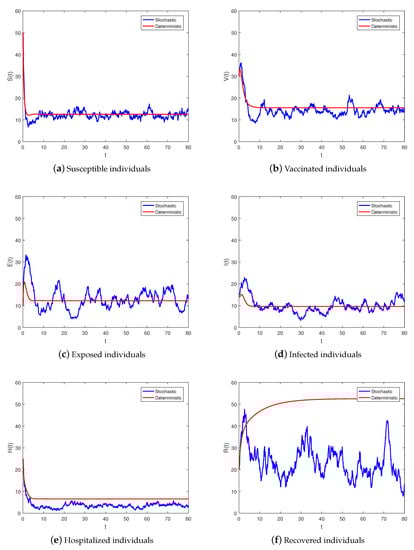
Figure 4.
Sample solution profiles of the system (3) correspond to its deterministic counterpart.
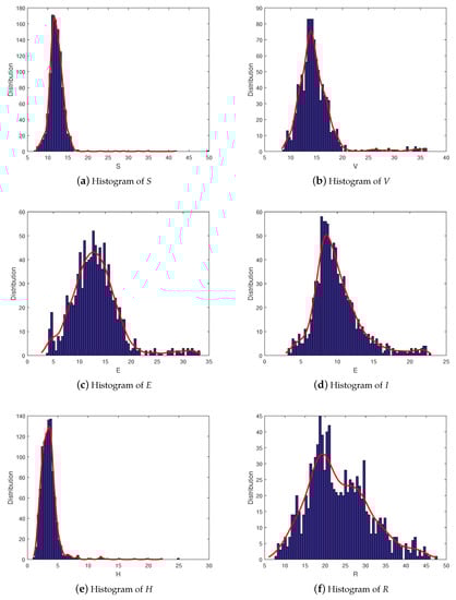
Figure 5.
Ergodic stationary distribution of (3).
Example 2.
In this case, the chosen parameter values are of the form: and . Similarly, the initial population sizes of the state variables are , whereas the intensities are given by . Considering the measles data and hence the estimated and fitted parameters, we find that exceeds unity. It is also explored that the model parameters taken in this example satisfy the premise of Theorem 3. We tested the model using this input, and the outcomes are displayed visually in Figure 4. The figure shows that the disease tends to stay inside the community, and the model exhibits a homogeneous stationary distribution in this situation.
From Theorem 3, there is a single stationary distribution of system (3). To numerically illustrate this statistical property, we present in Figure 4 and Figure 5, the trajectories and the associated joint density function for each class of the population. For a good visibility, we offer the and upper view of the aforementioned joint densities in Figure 6, Figure 7, Figure 8, Figure 9 and Figure 10. This indicates that the infection is still present in the population over time. We talk here about persistence in the mean of the epidemic. In Figure 4, we illustrate the continuation of all groups of the studied population. We remark that the stochastic trajectories fluctuate around the deterministic solution with reasonable distances according to magnitude of the noises.
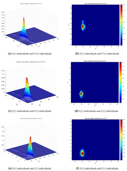
Figure 6.
The right panel of the figure shows the joint two-dimensional densities at of individuals , , and of system (3) correspond to data from Example 2—Test 2 (2nd column), where different colors depict the density sizes. The panel on the left demonstrates the 3D graph of the two-dimensional densities of , , and collectively (in this case, ).
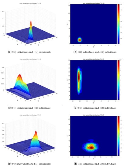
Figure 7.
The right panel of the figure shows the joint two-dimensional densities at of individuals , , , and of system (3) correspond to data from Example 2—Test 2 (2nd column), where different colors depict the density sizes. The panel on the left demonstrates the 3D graph of the two-dimensional densities of , , , and collectively (in this case, ).
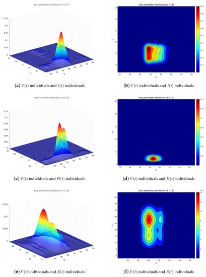
Figure 8.
The right panel of the figure shows the joint two-dimensional densities at of individuals , , , and of system (3) correspond to data from Example 2—Test 2 (2nd column), where different colors depict the density sizes. The panel on the left demonstrates the 3D graph of the two-dimensional densities of , , , and collectively (in this case, ).
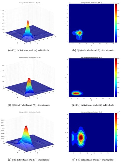
Figure 9.
The right panel of the figure shows the joint two-dimensional densities at of individuals , , , and of system (3) correspond to data from Example 2—Test 2 (2nd column), where different colors depict the density sizes. The panel on the left demonstrates the 3D graph of the two-dimensional densities of , , , and , collectively (in this case, ).
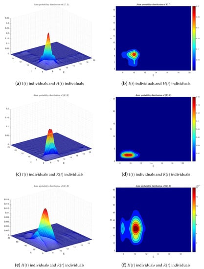
Figure 10.
(First part) The right panel of the figure shows that the joint two-dimensional densities at of individuals , , and of system (3) correspond to data from Example 2–Test 2 (2nd column), where different colors depict the density sizes. The panel on the left demonstrates the 3D graph of the two-dimensional densities of , , and collectively (in this case, ).
8. Conclusions and Future Research
In this study, we presented a detail analysis of a stochastic model that describes the spreading behavior of the measles virus while accounting for the white noises and the influence of immunizations. It is assumed that the randomness being used in the model is nonlinear, and that a person may lose the resistance after vaccination, implying that vaccination might create temporary protection against the disease. First of all, we formulated a deterministic model and then it was expanded to a stochastic model. It is shown that the stochastic model is both theoretically and practically viable by demonstrating that the model has a global solution which is positive and stochastically bounded. Next, we developed sufficient criteria for the disease’s elimination and permanence. Furthermore, the presence of a stationary distribution is examined by constructing a suitable Lyapunov function, wherein we noticed that the disease will persist for and that the illness will vanish from the community for . We simulated the model against the available data of measles in Pakistan during the first ten months of 2019, by using the conventional curve fitting methods, and the values of the parameters were calculated therein. These values of the parameters were used in simulating the model, and the theoretical findings of the research were evaluated and conclusions were made. Simulations of the study suggest that, in order to fully understand the dynamic behavior of the measles epidemic, time-delay must be included in such analyses, and that advancements in every vaccine campaign are unavoidable in order to stop or minimize the spreading of the disease.
We fit both stochastic and determinism models to known data on rubella in Pakistan during the first ten months of 2019, and the values of parameters were obtained using lsqcurvefit methods. These model parameters are used, and the threshold number, which is around 13, is determined. This demonstrates that measles is extremely harmful and might have a negative impact on this community if adequate control tactics are not implemented in time. It also suggests that, if no appropriate measures are implemented, the cases of the measles may increase in the coming years. To further reduce the transmission rate, health authorities and lawmakers must launch awareness campaigns, mass immunizations, particularly among youngsters, and, most crucially, care and treatment for people having chronic conditions. This was also discovered that serves as the most critical indicator to the threshold parameter; thus, lowering the disease spreading co-efficient (by lowering the household and sexual interactions of chronic patients with vulnerable) for acutely infected individuals who become chronic is also an effective control to reduce the spread of measles.
In the next research studies, the authors intend to use fractional calculus and modify this and the related model while utilizing different definitions of fractional derivatives such as Riesz, Caputo, Atangana–Baleanu, Caputo–Fabrizio, and many others for capturing the real dynamics of such and related diseases.
Author Contributions
Methodology, B.G. Formal analysis, B.G. Investigation, B.G. Data curation, A.K. and A.D.; Writing—original draft, B.G. and A.D. Writing—review and editing, A.K. Supervision, A.D. Project administration, A.K. All authors have read and agreed to the published version of the manuscript.
Funding
This research was sponsored by the Guangzhou Government Project under Grant No. 62216235, and the National Natural Science Foundation of China (Grant No. 12250410247).
Institutional Review Board Statement
Not applicable.
Informed Consent Statement
Not applicable.
Data Availability Statement
Not applicable.
Acknowledgments
Authors are grateful to the handling editor and reviewers for their constructive comments and remarks which helped to improve the quality of the manuscript.
Conflicts of Interest
The authors declare that they have no competing interests.
References
- Mose, O.F.; Sigey, J.K.; Okello, J.A.; Okwoyo, J.M.; Kang’ethe, G.J. Mathematical modeling on the control of measles by vaccination: Case study of KISII County, Kenya. SIJ Trans. Comput. Sci. Eng. Appl. CSEA 2014, 2, 61–69. [Google Scholar]
- Garba, S.M.; Safi, M.A.; Usaini, S. Mathematical model for assessing the impact of vaccination and treatment on measles transmission dynamics. Math. Meth. Appl. Sci. 2017, 40, 6371–6388. [Google Scholar] [CrossRef]
- Roberts, M.G.; Tobias, M.I. Predicting and preventing measles epidemic in New Zealand: Application of mathematical model. Epidem. Infect. 2000, 124, 279–287. [Google Scholar] [CrossRef] [PubMed]
- World Health Organization. Measles, Preprint. 2018. Available online: https://www.who.int/news-room/fact-sheets/detail/measles (accessed on 27 December 2019).
- Perry, R.T.; Halsey, N.A. The clinical significance of measles: A review. J. Infect. Dis. 2004, 189, S4–S16. [Google Scholar]
- Ejima, K.; Omori, R.; Aihara, K.; Nishiura, H. Real-time investigation of measles epidemics with estimate of vaccine efficacy. Int. J. Biol. Sci. 2012, 8, 620–629. [Google Scholar] [CrossRef]
- Mossong, J.; Muller, C.P. Modelling measles re-emergence as a result of waning of immunity in vaccinated populations. Vaccine 2003, 21, 4597–4603. [Google Scholar] [CrossRef]
- Bolarin, G. On the dynamical analysis of a new model for measles infection. Int. J. Math. Trends Technol. 2014, 7, 144–154. [Google Scholar] [CrossRef]
- Taiwo, L.; Idris, S.; Abubakar, A.; Nguku, P.; Nsubuga, P.; Gidado, S. Factors affecting access to information on routine immunization among mothers of under 5 children in Kaduna state Nigeria, 2015. Pan Afr. Med. J. 2017, 27, 186. [Google Scholar] [CrossRef]
- Center for Disease Control. Available online: https://www.cdc.gov/vaccines/vpd/measles/index.html (accessed on 26 January 2021).
- World Health Organization. Eastern Mediterranean Vaccine Action Plan 2016–2020: A Framework for Implementation of the Global Vaccine Action Plan (No. WHO-EM/EPI/353/E); World Health Organization, Regional Office for the Eastern Mediterranean: Cairo, Egypt, 2019. [Google Scholar]
- Dawn. Curbing Measles. Available online: https://www.dawn.com/news/1520931 (accessed on 7 December 2019).
- Memon, Z.; Qureshi, S.; Memon, B.R. Mathematical analysis for a new nonlinear measles epidemiological system using real incidence data from Pakistan. Eur. Phys. J. Plus 2020, 135, 1–21. [Google Scholar] [CrossRef]
- Asamoah, J.K.K.; Nyabadza, F.; Jin, Z.; Bonyah, E.; Khan, M.A.; Li, M.Y.; Hayat, T. Backward bifurcation and sensitivity analysis for bacterial meningitis transmission dynamics with a nonlinear recovery rate. Chaos Solitons Fractals 2020, 140, 110237. [Google Scholar] [CrossRef]
- Khan, F.M.; Khan, Z.U.; Lv, Y.-P.; Yusuf, A.; Din, A. Investigating of fractional order dengue epidemic model with ABC operator. Results Phys. 2021, 24, 104075. [Google Scholar] [CrossRef]
- Li, X.-P.; Bayatti, H.A.; Din, A.; Zeb, A. A vigorous study of fractional order COVID-19 model via ABC derivatives. Results Phys. 2021, 29, 104737. [Google Scholar] [CrossRef]
- Din, A.; Li, Y. Lévy noise impact on a stochastic hepatitis B epidemic model under real statistical data and its fractal–fractional Atangana–Baleanu order model. Phys. Scr. 2021, 96, 124008. [Google Scholar] [CrossRef]
- Srivastava, H.M.; Saad, K.M. Numerical simulation of the fractal-fractional Ebola virus. Fractal Fract. 2020, 4, 49. [Google Scholar] [CrossRef]
- Liu, P.; Ikram, R.; Khan, A. The measles epidemic model assessment under real statistics: An application of stochastic optimal control theory. Comput. Methods Biomech. Biomed. Eng. 2022, 26, 138–159. [Google Scholar] [CrossRef]
- Liu, G.; Qi, H.; Chang, Z.; Meng, X. Asymptotic stability of a stochastic May mutualism system. Comput. Math. Appl. 2020, 79, 735–745. [Google Scholar] [CrossRef]
- Tran, K.Q.; Yin, G. Optimal harvesting strategies for stochastic ecosystems. IET Control. Theory Appl. 2017, 11, 2521–2530. [Google Scholar] [CrossRef]
- Sabbar, Y.; Din, A. Probabilistic analysis of a marine ecological system with intense variability. Mathematics 2022, 10, 2262. [Google Scholar] [CrossRef]
- Din, A. The stochastic bifurcation analysis and stochastic delayed optimal control for epidemic model with general incidence function. Chaos Interdiscip. J. Nonlinear Sci. 2021, 31, 123101. [Google Scholar] [CrossRef]
- Khan, A.; Sabbar, Y. Stochastic modeling of the Monkeypox 2022 epidemic with cross-infection hypothesis in a highly disturbed environment. Math. Biosci. Eng. 2022, 19, 13560–13581. [Google Scholar] [CrossRef]
- Din, A.; Khan, A.; Sabbar, Y. Long-Term Bifurcation and Stochastic Optimal Control of a Triple-Delayed Ebola Virus Model with Vaccination and Quarantine Strategies. Fractal Fract. 2022, 6, 578. [Google Scholar] [CrossRef]
- Din, A.; Ain, Q.T. Stochastic Optimal Control Analysis of a Mathematical Model: Theory and Application to Non-Singular Kernels. Fractal Fract. 2022, 6, 279. [Google Scholar] [CrossRef]
- Omame, A.; Abbas, M.; Din, A. Global asymptotic stability, extinction and ergodic stationary distribution in a stochastic model for dual variants of SARS-CoV-2. Math. Comput. Simul. 2022, 204, 302–336. [Google Scholar] [CrossRef] [PubMed]
- Liu, P.; Rahman, M.u.; Din, A. Fractal fractional based transmission dynamics of COVID-19 epidemic model. Comput. Methods Biomech. Biomed. Eng. 2022, 25, 1852–1869. [Google Scholar] [CrossRef]
- Olumuyiwa, J.P.; Ojo, M.M.; Viriyapong, R.; Oguntolu, F.A. Mathematical model of measles transmission dynamics using real data from Nigeria. J. Differ. Equations Appl. 2022, 28, 753–770. [Google Scholar]
- Jin, X.; Jia, J. Qualitative study of a stochastic SIRS epidemic model with information intervention. Phys. A Stat. Mech. Appl. 2020, 547, 123866. [Google Scholar] [CrossRef]
- Rajasekar, S.P.; Pitchaimani, M. Qualitative analysis of stochastically perturbed SIRS epidemic model with two viruses. Chaos Solitons Fractals 2019, 118, 207–221. [Google Scholar] [CrossRef]
- Bao, K.; Zhang, Q. Stationary distribution and extinction of a stochastic SIRS epidemic model with information intervention. Adv. Differ. Equations 2017, 2017, 352. [Google Scholar] [CrossRef]
- Zhao, Y.N.; Jiang, D.Q. The threshold of a stochastic SIS epidemic model with vaccination. Appl. Math. Comput. 2014, 243, 718–727. [Google Scholar] [CrossRef]
- Khasminskii, R. Stochastic Stability of Differential Equations; Springer Science and Business Media: Berlin/Heidelberg, Germany, 2011. [Google Scholar]


Disclaimer/Publisher’s Note: The statements, opinions and data contained in all publications are solely those of the individual author(s) and contributor(s) and not of MDPI and/or the editor(s). MDPI and/or the editor(s) disclaim responsibility for any injury to people or property resulting from any ideas, methods, instructions or products referred to in the content. |
© 2023 by the authors. Licensee MDPI, Basel, Switzerland. This article is an open access article distributed under the terms and conditions of the Creative Commons Attribution (CC BY) license (https://creativecommons.org/licenses/by/4.0/).