
Stability and Hopf Bifurcation of a Class of Six-Neuron Fractional BAM Neural Networks with Multiple Delays

Abstract
:1. Introduction
2. Preliminaries
3. Local Stability of Equilibrium Point and Existence of Hopf Bifurcation
3.1. The Hopf Bifurcation of a System (3) with Time Delay as Parameter
- (1)
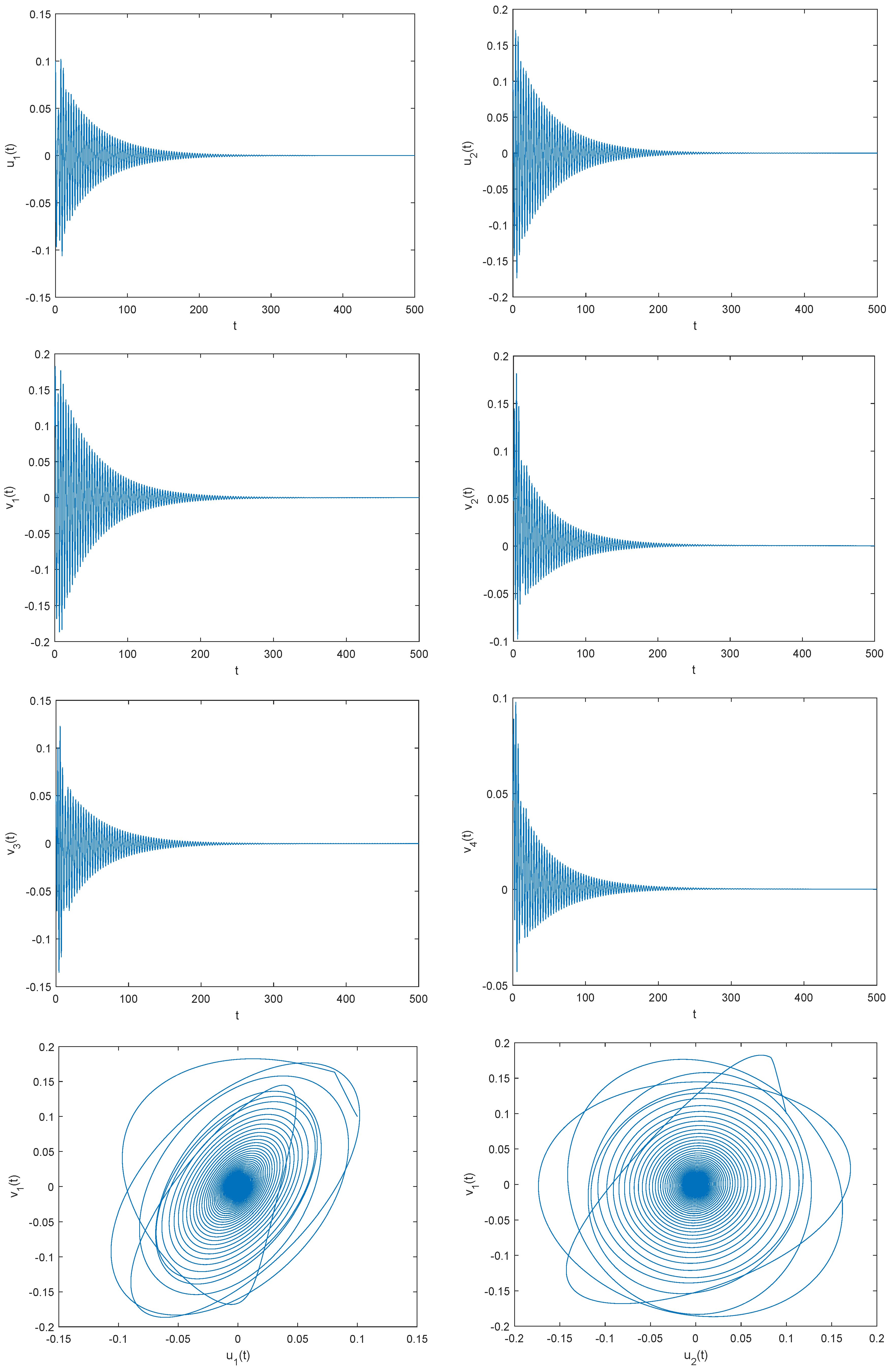
- If , then when , the zero equilibrium point of the fractional order system is asymptotically stable.
- (2)
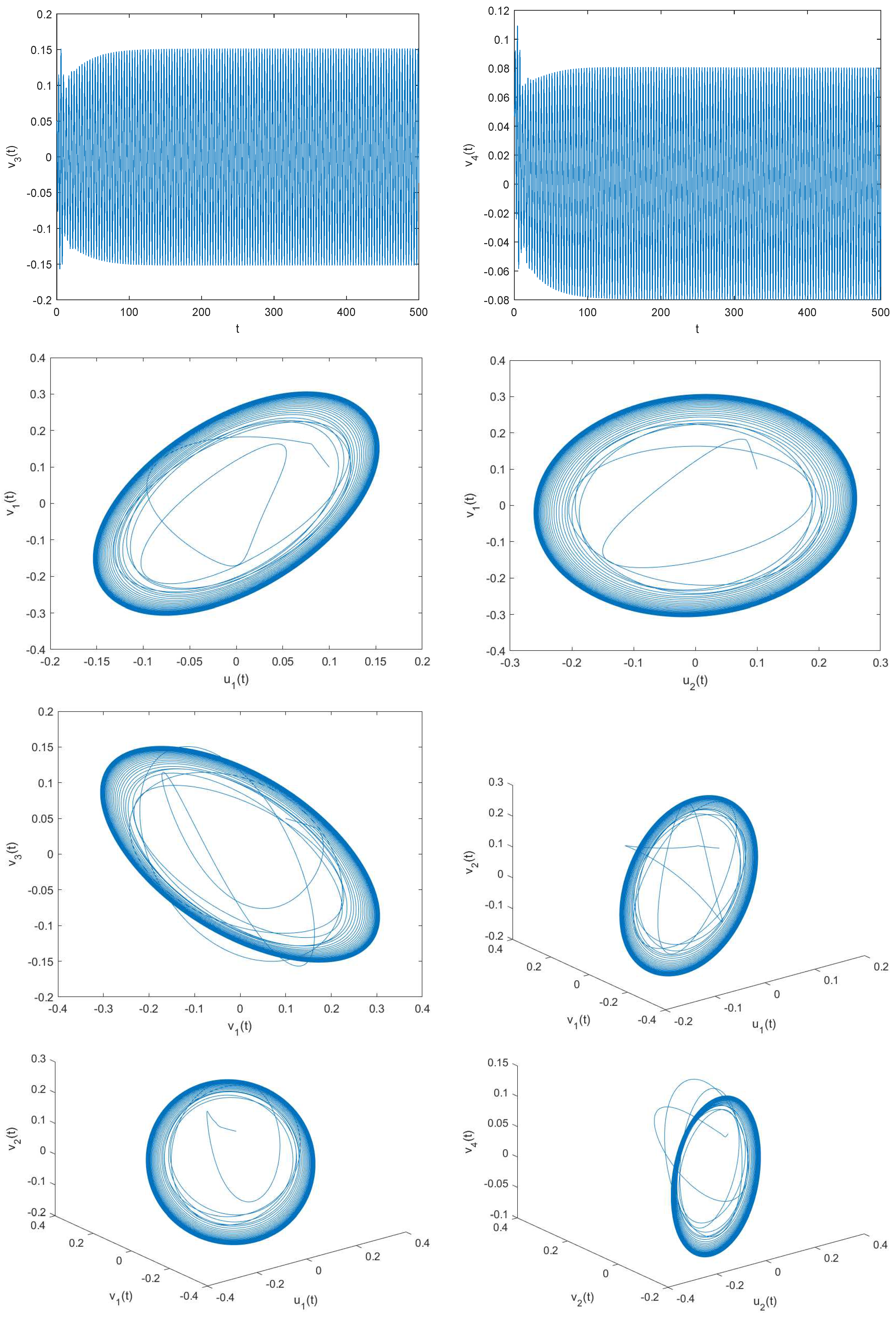
- If , then when , the zero equilibrium point of fractional order system loses stability and produces Hopf bifurcation.
3.2. The Hopf Bifurcation of a System (3) with Time Delay as Parameter
- (1)
- If , then when , the zero equilibrium point of the fractional order system is asymptotically stable.
- (2)
- If , then when , the zero equilibrium point of fractional order system loses stability and produces Hopf bifurcation.
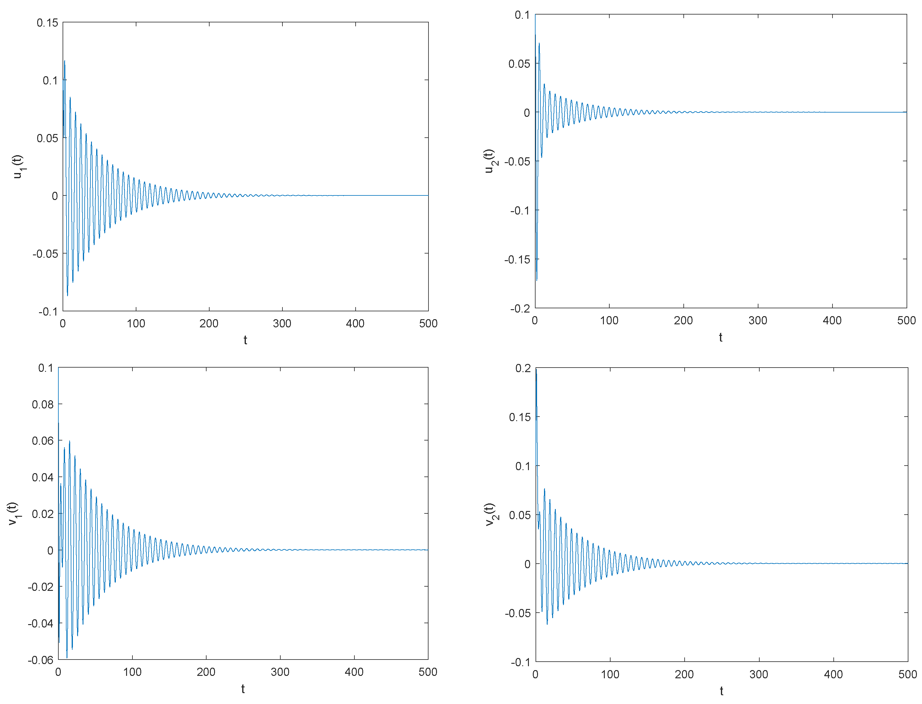
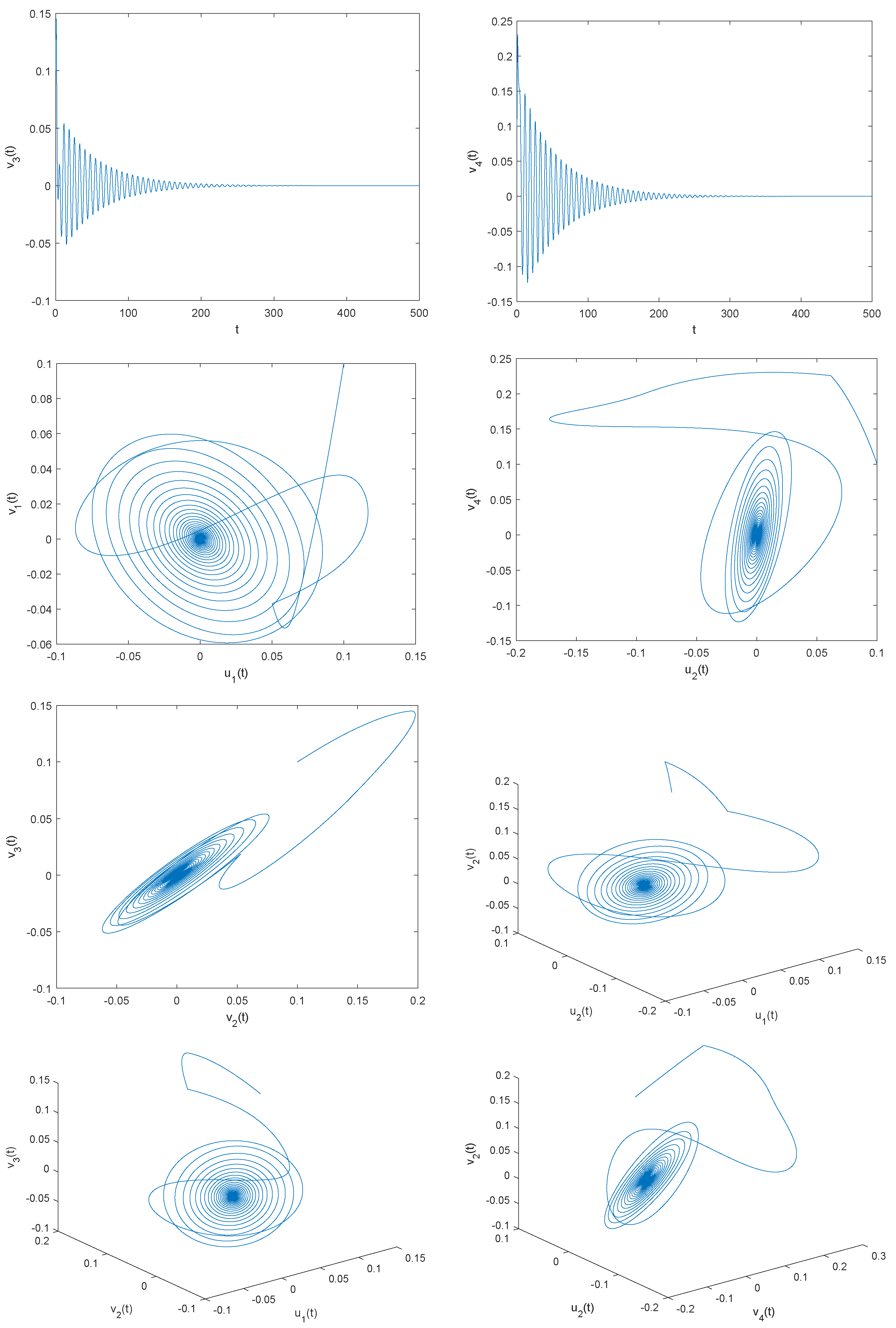
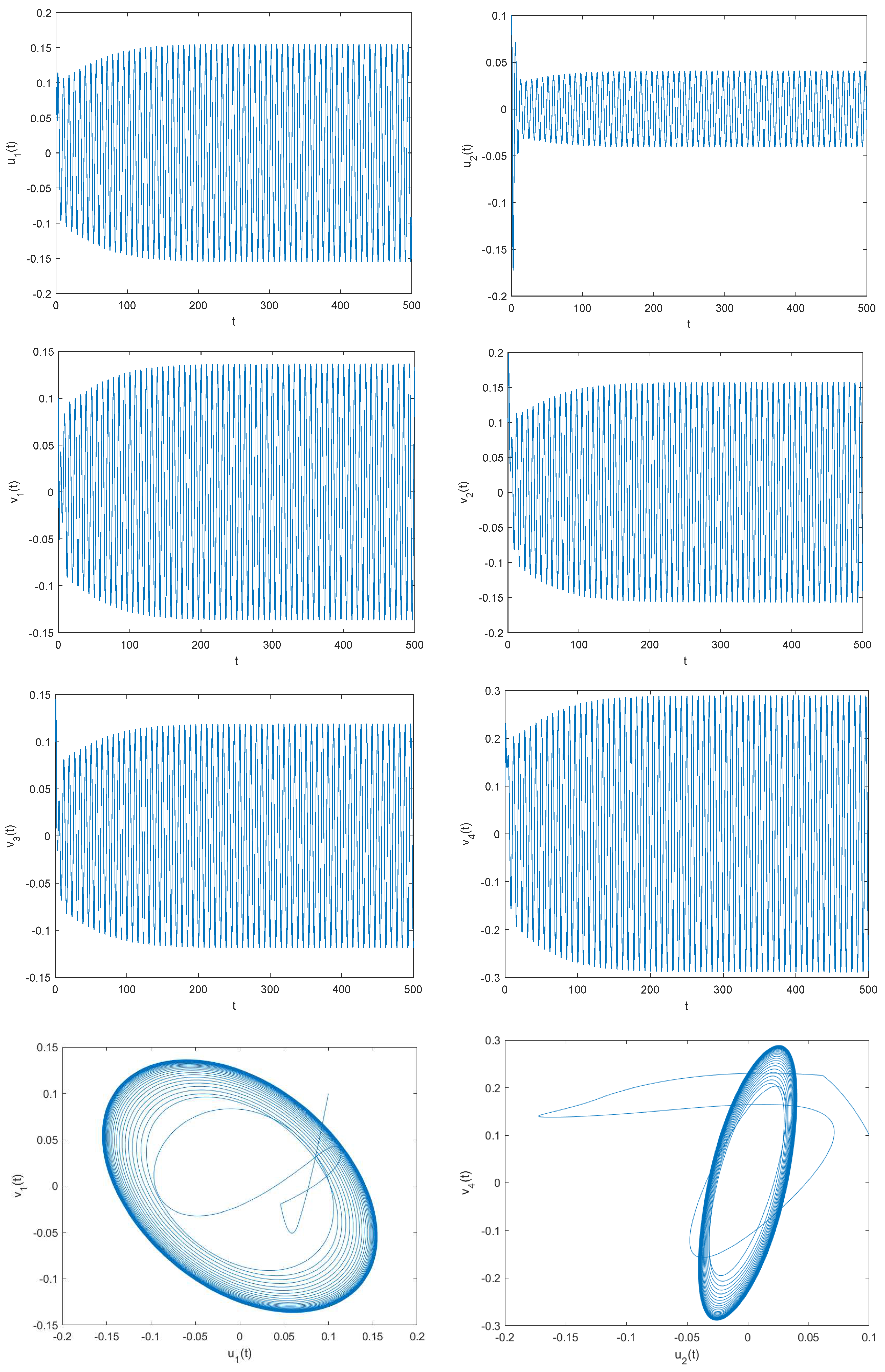
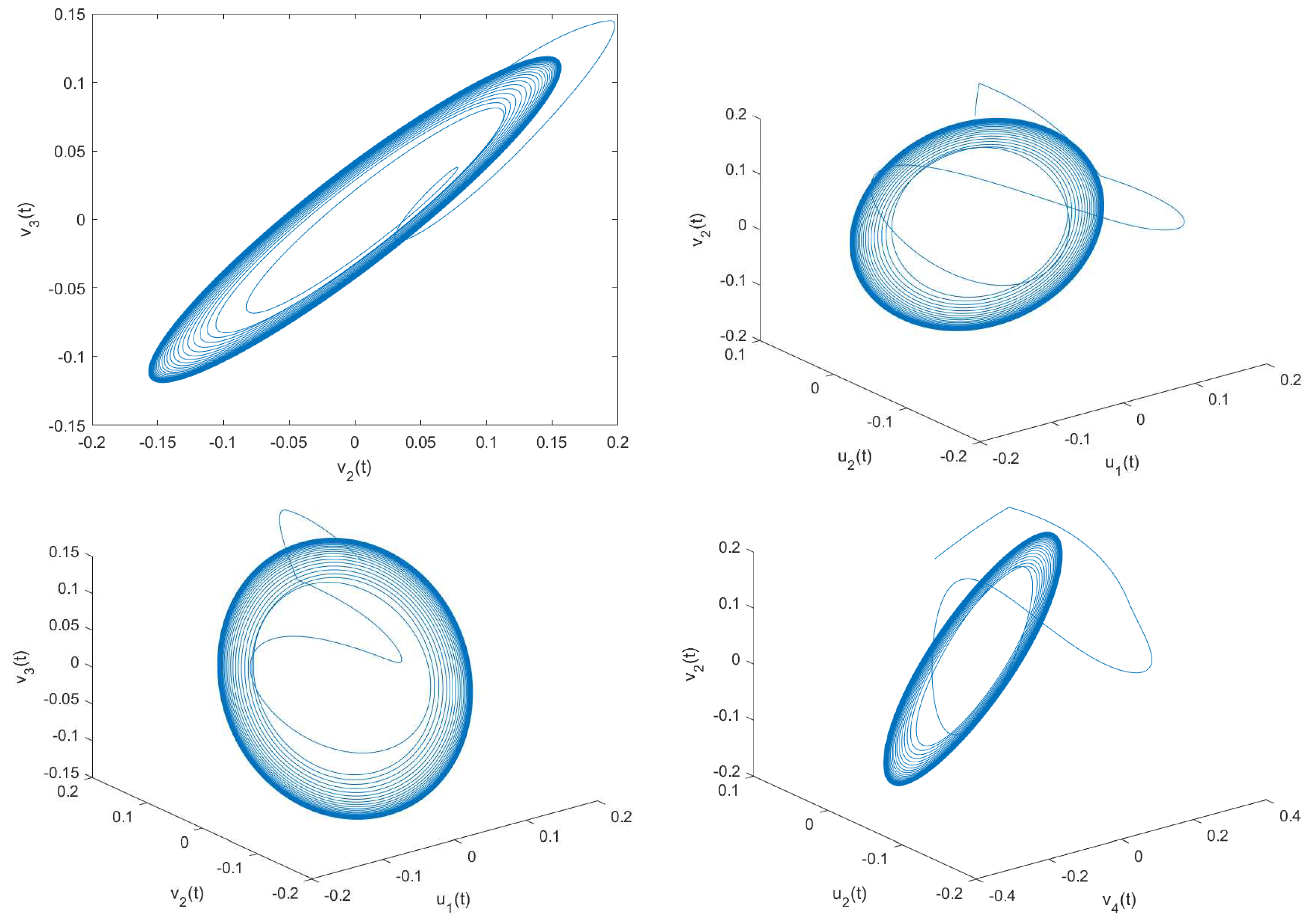
4. Numerical Examples
4.1. Example 1
4.2. Example 2
5. Conclusions
Author Contributions
Funding
Data Availability Statement
Conflicts of Interest
References
- Hopfield, J.J. Neural networks and physical systems with emergent collective computational abilities. Proc. Natl. Acad. Sci. USA 1982, 79, 2554–2558. [Google Scholar] [CrossRef] [PubMed]
- Hopfield, J.J. Neurons with graded response have collective computational properties like those of two-state neurons. Proc. Natl. Acad. Sci. USA 1984, 81, 3088–3092. [Google Scholar] [CrossRef] [PubMed]
- Kosko, B. Bidirectional associative memories. IEEE Trans. Syst. Man Cybern. 1988, 18, 49–60. [Google Scholar] [CrossRef]
- Song, Y.L.; Han, M.A.; Wei, J.J. Stability and Hopf bifurcation analysis on a simplified BAM neural network with delays. Phys. Nonlinear Phenom. 2005, 200, 185–204. [Google Scholar] [CrossRef]
- Yu, W.W.; Cao, J.D. Stability and Hopf bifurcation analysis on a four-neuron BAM neural network with time delays. Phys. Lett. A 2006, 351, 64–78. [Google Scholar] [CrossRef]
- Gopalsamy, K. Leakage delays in BAM. J. Math. Anal. Appl. 2007, 325, 1117–1132. [Google Scholar] [CrossRef]
- Cheng, Z.S.; Li, D.H.; Cao, J.D. Stability and Hopf bifurcation of a three-layer neural network model with delays. Neurocomputing 2016, 175, 355–370. [Google Scholar] [CrossRef]
- Matignon, D. Stability results for fractional differential equations with applications to control processing. Comput. Eng. Syst. Appl. 1996, 2, 963–968. [Google Scholar]
- Deng, W.H.; Li, C.P.; Lu, J.H. Stability analysis of linear fractional differential system with multiple time delays. Nonlinear Dyn. 2007, 48, 409–416. [Google Scholar] [CrossRef]
- Li, Y.; Chen, Y.Q.; Podlubny, I. Mittag-Leffler stability of fractional order nonlinear dynamic systems. Automatica 2009, 45, 1965–1969. [Google Scholar] [CrossRef]
- Li, Y.; Chen, Y.Q.; Podlubny, I. Stability of fractional-order nonlinear dynamic systems: Lyapunov direct method and generalized Mittag-Leffler stability. Comput. Math. Appl. 2009, 59, 1810–1821. [Google Scholar] [CrossRef] [Green Version]
- Huang, C.D.; Cao, J.D.; Xiao, M.; Alsaadi, F.E. Controlling bifurcation in a delayed fractional predator–prey system with incommensurate orders. Appl. Math. Comput. 2017, 293, 293–310. [Google Scholar] [CrossRef]
- Xu, C.J.; He, X.F.; Li, P.L. Global existence of periodic solutions in a six-neuron BAM neural network model with discrete delays. Neurocomputing 2011, 74, 3257–3267. [Google Scholar] [CrossRef]
- Xu, C.J.; Tang, X.H.; Liao, M.X. Stability and bifurcation analysis of a six-neuron BAM neural network model with discrete delays. Neurocomputing 2011, 74, 689–707. [Google Scholar] [CrossRef]
- Xu, C.J.; Liao, M.X.; Li, P.L.; Liu, Z. Bifurcation Properties for Fractional Order Delayed BAM Neural Networks. Cogn. Comput. 2021, 13, 322–356. [Google Scholar] [CrossRef]
- Xu, C.J.; Liu, Z.X.; Yao, L.Y.; Aouiti, C. Further exploration on bifurcation of fractional-order six-neuron bi-directional associative memory neural networks with multi-delays. Appl. Math. Comput. 2021, 410, 126458. [Google Scholar] [CrossRef]
- Xu, C.J.; Liu, Z.X.; Liao, M.X.; Xiao, Q.; Yuan, S. Fractional-order bidirectional associate memory (BAM) neural networks with multiple delays: The case of Hopf bifurcation. Math. Comput. Simul. 2021, 182, 471–494. [Google Scholar] [CrossRef]
- Huang, C.D.; Li, N.; Cao, J.D.; Hayat, T. Dynamical analysis of a delayed six-neuron BAM network. Complexity 2016, 21, 9–28. [Google Scholar] [CrossRef]
- Huang, C.D.; Cao, J.D.; Alofi, A.; AI-Mazrooei, A.; Elaiw, A.M. Dynamics and control in an (n + 2)-neuron BAM network with multiple delays. Nonlinear Dyn. 2017, 1, 313–336. [Google Scholar] [CrossRef]
- Huang, C.D.; Wang, J.; Chen, X.P.; Cao, J. Bifurcations in a fractional-order BAM neural network with four different delays. Neural Netw. Off. J. Int. Neural Netw. Soc. 2021, 141, 344–354. [Google Scholar] [CrossRef]
- Huang, C.D.; Liu, H.; Chen, Y.F.; Song, F. Dynamics of a fractional-order BAM neural network with leakage delay and communication delay. Fractals 2021, 29, 2150073. [Google Scholar] [CrossRef]
- Gunasekaran, N.; Thoiyab, N.M.; Zhu, Q.X.; Cao, J.D.; Muruganantham, P. New global asymptotic robust stability of dynamical delayed neural networks via intervalized interconnection matrices. IEEE Trans. Cybern. 2022, 52, 11794–11804. [Google Scholar] [CrossRef] [PubMed]
- Wu, Y.B.; Wang, Y.; Gunasekaran, N.; Vadivel, R. Almost Sure Consensus of Multi-Agent Systems: An Intermittent Noise. IEEE Trans. Circuits Syst. Express Briefs 2022, 69, 2897–2901. [Google Scholar] [CrossRef]
- Podlubny, I. Fractional Differential Equations; Academic Press: New York, NY, USA, 1999. [Google Scholar]
- Wang, T.S.; Wang, Y.; Cheng, Z.S. Stability and Hopf Bifurcation Analysis of a General Tri-diagonal BAM Neural Network with Delays. Neural Process. Lett. 2021, 53, 4571–4592. [Google Scholar] [CrossRef]
- Xiao, M.; Zheng, W.X.; Cao, J.D. Hopf Bifurcation of an (n + 1)-Neuron Bidirectional Associative Memory Neural Network Model with Delays. IEEE Trans. Neural Netw. Learn. Syst. 2013, 24, 118–132. [Google Scholar] [CrossRef]


Disclaimer/Publisher’s Note: The statements, opinions and data contained in all publications are solely those of the individual author(s) and contributor(s) and not of MDPI and/or the editor(s). MDPI and/or the editor(s) disclaim responsibility for any injury to people or property resulting from any ideas, methods, instructions or products referred to in the content. |
© 2023 by the authors. Licensee MDPI, Basel, Switzerland. This article is an open access article distributed under the terms and conditions of the Creative Commons Attribution (CC BY) license (https://creativecommons.org/licenses/by/4.0/).
Share and Cite
Li, B.; Liao, M.; Xu, C.; Chen, H.; Li, W. Stability and Hopf Bifurcation of a Class of Six-Neuron Fractional BAM Neural Networks with Multiple Delays. Fractal Fract. 2023, 7, 142. https://doi.org/10.3390/fractalfract7020142
Li B, Liao M, Xu C, Chen H, Li W. Stability and Hopf Bifurcation of a Class of Six-Neuron Fractional BAM Neural Networks with Multiple Delays. Fractal and Fractional. 2023; 7(2):142. https://doi.org/10.3390/fractalfract7020142
Chicago/Turabian StyleLi, Bingbing, Maoxin Liao, Changjin Xu, Huiwen Chen, and Weinan Li. 2023. "Stability and Hopf Bifurcation of a Class of Six-Neuron Fractional BAM Neural Networks with Multiple Delays" Fractal and Fractional 7, no. 2: 142. https://doi.org/10.3390/fractalfract7020142