First-Passage Times and Optimal Control of Integrated Jump-Diffusion Processes

Abstract

Let $Y\left(t\right)$ be a one-dimensional jump-diffusion process and $X\left(t\right)$ be defined by $\mathrm{d}X\left(t\right)=\rho \left[X\right(t),Y(t\left)\right]\mathrm{d}t$, where $\rho (·,·)$ is either a strictly positive or negative function. First-passage-time problems for the degenerate two-dimensional process $\left(X\right(t),Y(t\left)\right)$ are considered in the case when the process leaves the continuation region at the latest at the moment of the first jump, and the problem of optimally controlling the process is treated as well. A particular problem, in which $\rho \left[X\right(t),Y(t\left)\right]=Y\left(t\right)-X\left(t\right)$ and $Y\left(t\right)$ is a standard Brownian motion with jumps, is solved explicitly.

1. Introduction

Diffusion processes are used as models in various applications, in particular in neuroscience to emulate the dynamics of the membrane potential of a neuron [1]. Moreover, to take into account the spikes of the neuron, jump-diffusion processes have been proposed by Jahn et al. [2] and Melanson and Longtin [3], among others.

Now, diffusion and jump-diffusion processes both increase and decrease in any interval, however small. However, in some applications, it is not realistic to assume that the process can decrease or increase. For example, if $X\left(t\right)$ represents the wear of a machine at time t, the stochastic process $\left\{X\right(t),t\ge 0\}$ should increase with time.

One way to obtain a strictly increasing or decreasing process is to consider degenerate two-dimensional diffusion processes $\left(X\right(t),Y(t\left)\right)$ defined by

$$\begin{array}{ccc}\mathrm{d}X\left(t\right)& =& \rho \left[X\right(t),Y(t\left)\right]\mathrm{d}t,\end{array}$$

(1)

$$\begin{array}{ccc}\hfill \mathrm{d}Y\left(t\right)& =& f\left[Y\left(t\right)\right]\mathrm{d}t+{\left\{v\left[Y\right(t\left)\right]\right\}}^{1/2}\mathrm{d}B\left(t\right),\hfill \end{array}$$

(2)

where $\rho (·,·)$ is either a strictly positive or negative function and $\left\{B\right(t),t\ge 0\}$ is a standard Brownian motion. The functions f and v are such that $\left\{Y\right(t),t\ge 0\}$ is a diffusion process. When $\rho \left[X\right(t),Y(t\left)\right]=Y\left(t\right)$, the process $\left\{X\right(t),t\ge 0\}$ is called an integrated diffusion process. We can of course generalize the definition to the case when $\left\{Y\right(t),t\ge 0\}$ is a jump-diffusion process.

The author has published a number of papers on integrated diffusion processes; see, for instance, Lefebvre [4] for a recent one. Other papers on this topic include those by Lachal [5], Makasu [6], Metzler [7], Caravelli et al. [8] and Levy [9].

Next, we define the first-passage time

$$T(x,y)=inf\{t>0:(X\left(t\right),Y\left(t\right))\notin C\mid (X\left(0\right),Y\left(0\right))=(x,y)\in C\},$$

(3)

where C is a subset of ${\mathbb{R}}^2$.

Let $\varphi (\xi ,\eta ;x,y)$ be the joint probability density function (pdf) of the random vector $\left(X\right(t),Y(t\left)\right)$, with $\left(X\right(0),Y(0\left)\right)=(x,y)$. As is well known (see, for example, Cox and Miller [10], p. 247), the function $\varphi$ satisfies the Kolmogorov backward equation

$$\frac{1}{2}v\left(y\right){\varphi }_{yy}+f\left(y\right){\varphi }_y+\rho (x,y){\varphi }_x={\varphi }_t\mathrm{for}(x,y)\in C.$$

(4)

Moreover, the pdf $g(t;x,y)$ of the random variable $T(x,y)$ satisfies the same partial differential equation (PDE):

$$\frac{1}{2}v\left(y\right)g_{yy}+f\left(y\right)g_y+\rho (x,y)g_x=g_t$$

(5)

(subject to different boundary conditions). It follows that the moment-generating function of the random variable $T(x,y)$, namely

$$M(x,y;\alpha ):=E\left[e^{-\alpha T(x,y)}\right],$$

(6)

where $\alpha >0$, is a solution of the following PDE:

$$\frac{1}{2}v\left(y\right)M_{yy}+f\left(y\right)M_y+\rho (x,y)M_x=\alpha M\mathrm{for}(x,y)\in C,$$

(7)

where $M_{yy}:={\partial }^{2}M(x,y;\alpha )/\partial y^2$, etc. Furthermore, this equation is subject to the boundary condition

$$M(x,y;\alpha )=1\mathrm{for}(x,y)\notin C.$$

(8)

We now replace the diffusion process $\left\{Y\right(t),t\ge 0\}$ by the jump-diffusion process defined by

$$Y\left(t\right)=Y\left(0\right)+{\int }_0^{t}f\left[Y\left(s\right)\right]\mathrm{d}s+{\int }_0^t{\left\{v\left[Y\right(s\left)\right]\right\}}^{1/2}\mathrm{d}B\left(s\right)+\sum _{n=1}^{N\left(t\right)}{Z}_n,$$

(9)

where $\left\{N\right(t),t\ge 0\}$ is a Poisson process with rate $\lambda$. The random variables $Z_1$, $Z_2$, … are assumed to be independent and identically distributed (i.i.d.), and also independent of the Poisson process. We can state the following proposition.

Proposition 1.

The function $M(x,y;\alpha )$ satisfies the integro-differential equation (dropping the dependence on α from the notation)

$$\begin{array}{ccc}\hfill \alpha M(x,y)& =& \frac{1}{2}v\left(y\right)M_{yy}(x,y)+f\left(y\right)M_y(x,y)+\rho (x,y)M_x(x,y)\hfill \\ & & +\lambda \left\{{\int }_{-\infty }^{\infty }M(x,y+z)f_Z\left(z\right)\mathrm{d}z-M(x,y)\right\}\hfill \end{array}$$

(10)

for $(x,y)\in C$, where $f_Z\left(z\right)$ is the common density function of the $Z_n$s. As above, the equation is subject to the boundary condition (8).

Proof. 

This result is obtained by generalizing the infinitesimal generator of the jump-diffusion process $\left\{Y\right(t),t\ge 0\}$ in Kou and Wang [11] to the case when $f\left(y\right)$ and $v\left(y\right)$ are not necessarily constant functions. □

Remark 1.

See also the remark after the proof of Proposition 2.

There are still few explicit solutions to first-passage problems for jump-diffusion processes. Kou and Wang [11] obtained explicit formulae for the Laplace transform of the pdf of the first-passage time $\tau$ to a constant boundary for a Wiener process with jumps having a double exponential distribution. This model was generalized or modified in various papers. In Chen et al. [12], $\tau$ was the first-exit time from a finite interval, while in Yin et al. [13] the jumps were mixed-exponential random variables. Karnaukh [14] considered the case when the parameters of the Wiener process depend on a finite Markov chain. In Lefebvre [15], the jump sizes were assumed to be uniformly distributed, while in Abundo [16] the jumps (positive and/or negative) were of a constant size and the boundaries were time-dependent. Because obtaining exact analytical solutions to such problems is difficult, some authors presented numerical techniques to obtain the quantities of interest; see, for example, Belkaid and Utzet [17].

Di Crescenzo et al. [18] computed bounds for first-crossing-time probabilities of a Wiener process with random jumps driven by a counting process. Fernández et al. [19] proposed algorithms to compute double-barrier first-passage-time probabilities of a jump-diffusion process with an arbitrary jump size distribution.

D’Onofrio and Lanteri [20] obtained numerical approximations for the density functions of first-passage times in the case of diffusion processes with state-dependent jumps. Finally, in Lefebvre [21], the author was able to obtain exact solutions to optimal control problems for Wiener processes with exponential jumps.

In the current paper, explicit results will be presented for the first-passage time of a two-dimensional jump-diffusion process.

In the next section, the special case when the two-dimensional process $\left(X\right(t),Y(t\left)\right)$ is killed at the latest at the moment of the first jump, will be considered. We are also interested in the mean value of $T(x,y)$, as well as in the probability that $\left(X\right(t),Y(t\left)\right)$ will leave the continuation region through a given part of its boundary $\partial C$. In Section 3, the problem of maximizing or minimizing the time the controlled version of the process $\left(X\right(t),Y(t\left)\right)$ spends in the continuation region C will be treated. A particular problem will be solved explicitly in Section 4. Finally, we will conclude with a few remarks in Section 5.

2. Killed Processes

Assume that the random variables $Z_1,Z_2,\dots$ are such that no overshoot is possible. That is, the degenerate two-dimensional jump-diffusion process $\left(X\right(t),Y(t\left)\right)$ cannot jump over the boundary of the continuation region C. Let $m(x,y):=E\left[T\right(x,y\left)\right]$ and

$$p(x,y):=P[(X\left(T\right),Y\left(T\right))\in \partial C_0\mid X\left(0\right)=x,Y\left(0\right)=y],$$

(11)

where $\partial C_0\subset \partial C$. We have the following corollaries.

Corollary 1.

The function $m(x,y)$ satisfies the integro-differential equation

$$\begin{array}{ccc}\hfill -1& =& \frac{1}{2}v\left(y\right)m_{yy}(x,y)+f\left(y\right)m_y(x,y)+\rho (x,y)m_x(x,y)\hfill \\ & & +\lambda \left\{{\int }_{-\infty }^{\infty }m(x,y+z)f_Z\left(z\right)\mathrm{d}z-m(x,y)\right\}\hfill \end{array}$$

(12)

for $(x,y)\in C$, subject to the boundary condition

$$m(x,y)=0\mathit{for}(x,y)\notin C.$$

(13)

Proof. 

It follows from the expansion of $M(x,y;\alpha )$ into an infinite series (see Cox and Miller [10]):

$$\begin{array}{ccc}\hfill M(x,y;\alpha )& :=& E\left[e^{-\alpha T(x,y)}\right]=E\left[1-\alpha T(x,y)+\frac{1}{2}{\alpha }^2{T}^2(x,y)-\dots \right]\hfill \end{array}$$

(14)

$$\begin{array}{ccc}& =& 1-\alpha m(x,y)+\frac{1}{2}{\alpha }^{2}E\left[T^2(x,y)\right]-\dots \hfill \end{array}$$

(15)

Notice that in our case, $E\left[T^n(x,y)\right]$ will exist for any $n\in \{1,2,\dots \}$ because of Equation (18) below. □

Corollary 2.

The probability $p(x,y)$ is a solution of the integro-differential equation

$$\begin{array}{ccc}\hfill 0& =& \frac{1}{2}v\left(y\right)p_{yy}(x,y)+f\left(y\right)p_y(x,y)+\rho (x,y)p_x(x,y)\hfill \\ & & +\lambda \left\{{\int }_{-\infty }^{\infty }p(x,y+z)f_Z\left(z\right)\mathrm{d}z-p(x,y)\right\}\hfill \end{array}$$

(16)

for $(x,y)\in C$. Moreover, the boundary condition is

$$p(x,y)=\left\{\begin{array}{cc}1& \mathrm{if}(x,y)\in \partial C_0,\hfill \\ 0& \mathrm{if}(x,y)\in \partial D,\hfill \end{array}\right.$$

(17)

where $\partial D:=\partial C\backslash \partial C_0$.

In this paper, we consider the special case when the random variable $Z_1$ is such that the process $\left(X\right(t),Y(t\left)\right)$ will leave the continuation region C at the latest at the moment ${\tau }_1$ of the first event of the Poisson process. Let $T_0(x,y)$ be the random variable that corresponds to $T(x,y)$ when $\lambda =0$. We can write that

$$T(x,y)=min\{T_0,{\tau }_1\},$$

(18)

where ${\tau }_1$ has an exponential distribution with parameter $\lambda$. Furthermore, the sum in Equation (9) can be replaced by $Z_1{\mathbb{1}}_{\left\{N\right(t)>0\}}$, where ${\mathbb{1}}_{\left\{N\right(t)>0\}}$ is the indicator variable of the event $\left\{N\right(t)>0\}$, and the equation is valid for $t\in [0,T(x,y\left)\right]$. We can say that the process $\left(X\right(t),Y(t\left)\right)$ is killed at time $T(x,y)$.

An application of the above problem is the following: as mentioned in Section 1, a more realistic model for the wear of a machine is the degenerate two-dimensional process $\left(X\right(t),Y(t\left)\right)$ defined in Equations (1) and (2), when $\rho (·,·)$ is a strictly increasing function. Rishel [22] proposed this model (in n dimensions) in the context of an optimal control problem. If $X\left(t\right)$ denotes the remaining amount of deterioration that a device can undergo before it must be repaired or replaced, then $\rho (·,·)$ should be strictly negative instead. Moreover, the remaining lifetime of the device is the first-passage time to zero or to a level at which it is considered worn out.

Now, many electronic devices, especially mobile phones, are often replaced as soon as they break down, rather than being repaired. A mobile phone failure can be seen as a jump from the current value of $X\left(t\right)$ to zero, so that the device is killed at the time of the jump. It is also possible that the device will be replaced before a failure occurs, due to normal wear and tear or because it has become obsolete. Thus, deterioration could also include the age of the device.

Similarly, in the case of humans, the downward jump to zero could occur during a massive heart attack or stroke.

Because we assume that $(x,y+z)\in \partial C$ for any possible value z of the random variable Z, the integro-differential Equations (10) and (12) become, respectively, the partial differential equations

$$\begin{array}{ccc}\hfill \alpha M(x,y)& =& \frac{1}{2}v\left(y\right)M_{yy}(x,y)+f\left(y\right)M_y(x,y)+\rho (x,y)M_x(x,y)\hfill \\ & & +\lambda [1-M(x,y\left)\right]\hfill \end{array}$$

(19)

and

$$-1=\frac{1}{2}v\left(y\right)m_{yy}(x,y)+f\left(y\right)m_y(x,y)+\rho (x,y)m_x(x,y)-\lambda m(x,y).$$

(20)

In the case of Equation (16), if $(x,y+z)\in \partial C_0$$\forall z$, then

$$0=\frac{1}{2}v\left(y\right)p_{yy}(x,y)+f\left(y\right)p_y(x,y)+\rho (x,y)p_x(x,y)+\lambda [1-p(x,y)],$$

(21)

whereas, we have

$$0=\frac{1}{2}v\left(y\right)p_{yy}(x,y)+f\left(y\right)p_y(x,y)+\rho (x,y)p_x(x,y)-\lambda p(x,y)$$

(22)

if $(x,y+z)\in \partial D$$\forall z$. If $(x,y+z)$ belongs to $\partial C_0$ for some values of z, and to $\partial D$ for other values of z, then the integral in Equation (16) is replaced by

$${\int }_{-\infty }^{\infty }{\mathbb{1}}_{\{(x,y+z)\in \partial C_0\}}{f}_Z\left(z\right)\mathrm{d}z=P[(x,y+Z)\in \partial C_0].$$

(23)

Solving integro-differential equations explicitly and exactly is not an easy task. In Section 4, an example of a problem that we can indeed solve analytically will be presented. As above, the integro-differential equations will be reduced to PDE’s, and the method of similarity solutions will be used to transform these PDE’s into ordinary differential equations.

3. Optimal Control

In this section, we consider a controlled version of the two-dimensional process $\left(X\right(t),Y(t\left)\right)$:

$$\begin{array}{ccc}\hfill X_u\left(t\right)& =& X_u\left(0\right)+{\int }_0^t\rho [X_u\left(s\right),Y_u\left(s\right)]\mathrm{d}s,\hfill \\ \hfill Y_u\left(t\right)& =& Y_u\left(0\right)+{\int }_0^{t}bu[X_u\left(s\right),Y_u\left(s\right)]\mathrm{d}s+{\int }_0^{t}f\left[Y_u\left(s\right)\right]\mathrm{d}s\hfill \end{array}$$

(24)

$$\begin{array}{ccc}& & +{\int }_0^t{\left\{v\left[Y_u\left(s\right)\right]\right\}}^{1/2}\mathrm{d}B\left(s\right)+\sum _{n=1}^{N\left(t\right)}{Z}_n,\hfill \end{array}$$

(25)

where $u(·,·)$ is the control variable, which is assumed to be a continuous function, and b is a non-zero constant. The aim is to find the value of the control that minimizes the expected value of the cost function

$$J(x,y):={\int }_0^{T(x,y)}\left\{\frac{1}{2}q{u}^2[X_u\left(t\right),Y_u\left(t\right)]+\theta \right\}\mathrm{d}t,$$

(26)

where $q>0$ and $\theta$ are constants. If the parameter $\theta$ is positive (respectively negative), the optimizer must try to minimize (respectively maximize) the time spent by the controlled process in the continuation C, taking the quadratic control costs into account. This type of problem is known as a homing problem; see Whittle [23] and/or [24].

To solve the above problem, we can make use of dynamic programming. We define the value function

$$F(x,y)=\underset{\begin{array}{c}u[X_u\left(t\right),Y_u\left(t\right)]\\ t\in [0,T(x,y\left)\right)\end{array}}{inf}E\left[J(x,y)\right].$$

(27)

That is, $F(x,y)$ is the expected cost (or reward, if it is negative) obtained by choosing the optimal value of the control variable in the interval $[0,T(x,y\left)\right)$.

Proposition 2.

The value function $F(x,y)$ satisfies the second-order, non-linear partial integro-differential equation

$$\begin{array}{ccc}\hfill 0& =& \theta -\frac{1}{2}\frac{b^2}{q}{F}_y^2(x,y)+\rho (x,y)F_x(x,y)+f\left(y\right)F_y(x,y)+\frac{1}{2}v\left(y\right)F_{yy}(x,y)\hfill \\ & & +\lambda \left\{{\int }_{-\infty }^{\infty }F(x,y+z)f_Z\left(z\right)\mathrm{d}z-F(x,y)\right\}.\hfill \end{array}$$

(28)

Moreover, we have the boundary condition

$$F(x,y)=0\mathit{for}(x,y)\notin C.$$

(29)

Proof. 

First, thanks to Bellman’s principle of optimality, we can write that

$$\begin{array}{ccc}\hfill F(x,y)& =& \underset{\begin{array}{c}u[X_u\left(t\right),Y_u\left(t\right)]\\ 0\le t\le \Delta t\end{array}}{inf}E[{\int }_0^{\Delta t}\left\{\frac{1}{2}q{u}^2[X_u\left(t\right),Y_u\left(t\right)]+\theta \right\}\mathrm{d}t\hfill \\ & & +F(x+\rho (x,y)\Delta t,y+[f\left(y\right)+bu(x,y)]\Delta t+v^{1/2}\left(y\right)B(\Delta t)\hfill \\ & & +\sum _{n=1}^{N(\Delta t)}{Z}_n)+o(\Delta t)]\hfill \end{array}$$

(30)

$$\begin{array}{ccc}& =& \underset{\begin{array}{c}u[X_u\left(t\right),Y_u\left(t\right)]\\ 0\le t\le \Delta t\end{array}}{inf}E[\left\{\frac{1}{2}q{u}^2(x,y)+\theta \right\}\Delta t\hfill \\ & & +F(x+\rho (x,y)\Delta t,y+[f\left(y\right)+bu(x,y)]\Delta t+v^{1/2}\left(y\right)B(\Delta t)\hfill \\ & & +\sum _{n=1}^{N(\Delta t)}{Z}_n)+o(\Delta t)].\hfill \end{array}$$

(31)

Next, let

$$\xi :=x+\rho (x,y)\Delta t$$

(32)

and

$$\eta :=y+[f\left(y\right)+bu(x,y)]\Delta t+v^{1/2}\left(y\right)B(\Delta t).$$

(33)

We have

$$E\left[F\left(\xi ,\eta +\sum _{n=1}^{N(\Delta t)}{Z}_n\right)\right]=E\left[E\left[F\left(\xi ,\eta +\sum _{n=1}^{N(\Delta t)}{Z}_n\right)|N(\Delta t)\right]\right].$$

(34)

Since $N(\Delta t)$ has a Poisson distribution with parameter $\lambda \Delta t$, we can write that

$$P[N(\Delta t)=1]=\lambda \Delta t{e}^{-\lambda \Delta t}=\lambda \Delta t+o(\Delta t)$$

(35)

and

$$P\left[N\right(\Delta t)\ge 2]=o(\Delta t).$$

(36)

Hence,

$$E\left[F\left(\xi ,\eta +\sum _{n=1}^{N(\Delta t)}{Z}_n\right)\right]=E\left[F(\xi ,\eta )\right](1-\lambda \Delta t)+E\left[F(\xi ,\eta +Z_1)\right]\lambda \Delta t+o(\Delta t).$$

(37)

Now, assuming that $F(x,y)$ is twice differentiable with respect to x and to y, making use of Taylor’s formula for functions of two variables, we obtain that

$$\begin{array}{ccc}& & F\left(x+\rho (x,y)\Delta t,y+[f\left(y\right)+bu(x,y)]\Delta t+v^{1/2}\left(y\right)B(\Delta t)\right)\hfill \\ & & =F(x,y)+\rho (x,y)\Delta t{F}_x(x,y)\hfill \\ & & +\left\{[f\left(y\right)+bu(x,y)]\Delta t+v^{1/2}\left(y\right)B(\Delta t)\right\}{F}_y(x,y)\hfill \\ & & +\frac{1}{2}{[\rho (x,y)\Delta t]}^2{F}_{xx}(x,y)\hfill \\ & & +\frac{1}{2}{\left\{[f\left(y\right)+bu(x,y)]\Delta t+v^{1/2}\left(y\right)B(\Delta t)\right\}}^2{F}_{yy}(x,y)\hfill \\ & & +[\rho (x,y)\Delta t]\left\{[f\left(y\right)+bu(x,y)]\Delta t+v^{1/2}\left(y\right)B(\Delta t)\right\}{F}_{xy}(x,y)\hfill \\ & & +o(\Delta t).\hfill \end{array}$$

(38)

Furthermore, we have $E\left[B\right(\Delta t\left)\right]=0$ and $E\left[B^2(\Delta t)\right]=V\left[B(\Delta t)\right]=\Delta t$, which implies that

$$\begin{array}{ccc}\hfill E\left[F(\xi ,\eta )\right](1-\lambda \Delta t)& =& F(x,y)+\rho (x,y)\Delta t{F}_x(x,y)\hfill \\ & & +[f\left(y\right)+bu(x,y)]\Delta t{F}_y(x,y)+\frac{1}{2}v\left(y\right)\Delta t{F}_{yy}(x,y)\hfill \\ & & -F(x,y)\lambda \Delta t+o(\Delta t).\hfill \end{array}$$

(39)

Similarly, we find that

$$\begin{array}{ccc}\hfill E\left[F(\xi ,\eta +Z_1)\right]\lambda \Delta t& =& E\left[F(x,y+Z_1)\right]\lambda \Delta t+o(\Delta t)\hfill \\ & =& \lambda \Delta t{\int }_{-\infty }^{\infty }F(x,y+z)f_Z\left(z\right)\mathrm{d}z+o(\Delta t).\hfill \end{array}$$

(40)

Indeed, by independence, we have

$$E\left[F(\xi ,\eta +Z_1)\right]={\int }_{-\infty }^{\infty }E\left[F(\xi ,\eta +z)\right]f_Z\left(z\right)\mathrm{d}z.$$

(41)

Let $w:=y+z$. We compute

$$\begin{array}{ccc}& & E\left[F\left(x+\rho (x,y)\Delta t,y+[f\left(y\right)+bu(x,y)]\Delta t+v^{1/2}\left(y\right)B(\Delta t)+z\right)\right]\hfill \\ & & =F(x,w)+\rho (x,y)\Delta t{F}_x(x,w)+[f\left(y\right)+bu(x,y)]\Delta t{F}_w(x,w)\hfill \\ & & +\frac{1}{2}v\left(y\right)\Delta t{F}_{ww}(x,w)+o(\Delta t),\hfill \end{array}$$

(42)

so that

$$\begin{array}{ccc}& & E\left[F\left(x+\rho (x,y)\Delta t,y+[f\left(y\right)+bu(x,y)]\Delta t+v^{1/2}\left(y\right)B(\Delta t)+z\right)\right]\lambda \Delta t\hfill \\ & & =F(x,w)\lambda \Delta t+o(\Delta t)=F(x,y+z)\lambda \Delta t+o(\Delta t).\hfill \end{array}$$

(43)

Thus,

$$\begin{array}{ccc}\hfill E\left[F(\xi ,\eta +Z_1)\right]\lambda \Delta t& =& {\int }_{-\infty }^{\infty }\left[F(x,y+z)\lambda \Delta t+o(\Delta t)\right]f_Z\left(z\right)\mathrm{d}z\hfill \\ & =& E\left[F(x,y+Z_1)\right]\lambda \Delta t+o(\Delta t).\hfill \end{array}$$

(44)

From Equation (31) and the above results, we deduce that

$$\begin{array}{ccc}\hfill 0& =& \underset{\begin{array}{c}u[X_u\left(t\right),Y_u\left(t\right)]\\ 0\le t\le \Delta t\end{array}}{inf}\{\left[\frac{1}{2}q{u}^2(x,y)+\theta \right]\Delta t+\rho (x,y)\Delta t{F}_x(x,y)\hfill \\ & & +[f\left(y\right)+bu(x,y)]\Delta t{F}_y(x,y)+\frac{1}{2}v\left(y\right)\Delta t{F}_{yy}(x,y)\hfill \\ & & -F(x,y)\lambda \Delta t+\lambda \Delta t{\int }_{-\infty }^{\infty }F(x,y+z)f_Z\left(z\right)\mathrm{d}z+o(\Delta t)\}.\hfill \end{array}$$

(45)

Dividing both sides of the above equation by $\Delta t$ and letting $\Delta t$ decrease to zero, we obtain the dynamic programming equation

$$\begin{array}{ccc}\hfill 0& =& \underset{u(x,y)}{inf}\{\frac{1}{2}q{u}^2(x,y)+\theta +\rho (x,y)F_x(x,y)\hfill \\ & & +[f\left(y\right)+bu(x,y)]F_y(x,y)+\frac{1}{2}v\left(y\right)F_{yy}(x,y)\hfill \\ & & -\lambda F(x,y)+\lambda {\int }_{-\infty }^{\infty }F(x,y+z)f_Z\left(z\right)\mathrm{d}z\}.\hfill \end{array}$$

(46)

From the preceding equation, we find that the optimal control $u^{*}(x,y)$ can be expressed as follows:

$$u^{*}(x,y)=-\frac{b}{q}{F}_y(x,y).$$

(47)

Substituting the optimal control into Equation (46), we obtain Equation (28).

Finally, the boundary condition (29) follows at once from the definition of $F(x,y)$, since $T(x,y)=0$ if $(x,y)\notin C$. □

Remark 2.

Suppose that we set $u[X_u\left(s\right),Y_u\left(s\right)]$ equal to zero in Equation (25) and that we replace the cost function $J(x,y)$ defined in Equation (26) by

$$J_0(x,y,t_0):={\int }_{t_0}^{\infty }{e}^{-\alpha t}g(t;t_0,x,y)\mathrm{d}t,$$

(48)

where $g(t;t_0,x,y)$ is the pdf of $T(x,y)$ when the starting time is equal to $t_0$. Then, since $J_0(x,y,t_0)$ is actually a deterministic function, we may write that

$$\mathsf{\Phi }(x,y,t_0):=E\left[J_0(x,y,t_0)\right]=J_0(x,y,t_0)=M(x,y,t_0;\alpha ).$$

(49)

Proceeding as in the above proof, we find that

$$\begin{array}{ccc}\hfill 0& =& e^{-\alpha t_0}g(t_0;t_0,x,y)+{\mathsf{\Phi }}_{t_0}(x,y,t_0)+\rho (x,y){\mathsf{\Phi }}_x(x,y,t_0)+f\left(y\right){\mathsf{\Phi }}_y(x,y,t_0)\hfill \\ & & +\frac{1}{2}v\left(y\right){\mathsf{\Phi }}_{yy}(x,y,t_0)-\lambda \mathsf{\Phi }(x,y,t_0)+\lambda {\int }_{-\infty }^{\infty }\mathsf{\Phi }(x,y+z,t_0)f_Z\left(z\right)\mathrm{d}z.\hfill \end{array}$$

(50)

We have $g(t_0;t_0,x,y)=0$ for $(x,y)\in C$. Moreover, using the Leibniz integral rule,

$$\begin{array}{ccc}\hfill {\mathsf{\Phi }}_{t_0}(x,y,t_0)& =& -e^{-\alpha t_0}g(t_0;t_0,x,y)+{\int }_{t_0}^{\infty }{e}^{-\alpha t}{g}_{t_0}(t;t_0,x,y)\mathrm{d}t\hfill \\ & =& 0-{\int }_{t_0}^{\infty }{e}^{-\alpha t}{g}_t(t;t_0,x,y)\mathrm{d}t\hfill \\ & =& -e^{-\alpha t}g(t;t_0,x,y){|}_{t_0}^{\infty }-\alpha {\int }_{t_0}^{\infty }{e}^{-\alpha t}g(t;t_0,x,y)\mathrm{d}t\hfill \\ & =& -\alpha M(x,y,t_0;\alpha ),\hfill \end{array}$$

(51)

where we used the fact that $g_{t_0}(t;t_0,x,y)=-g_t(t;t_0,x,y)$ because the two-dimensional process $(X_u\left(t\right),Y_u\left(t\right))$ is time-invariant. Hence, setting $t_0$ equal to zero, we retrieve Equation (10).

In the case of the killed processes considered in Section 2, the integro-differential Equation (28) reduces to the non-linear PDE

$$\begin{array}{ccc}\hfill 0& =& \theta -\frac{1}{2}\frac{b^2}{q}{F}_y^2(x,y)+\rho (x,y)F_x(x,y)+f\left(y\right)F_y(x,y)+\frac{1}{2}v\left(y\right)F_{yy}(x,y)\hfill \\ & & -\lambda F(x,y).\hfill \end{array}$$

(52)

The boundary condition remains the one in Equation (29).

In the next section, a particular problem will be treated. We will find the exact optimal control when the parameter $\lambda$ is equal to zero, so that there are no jumps, and a numerical solution will be computed in the case when $\lambda >0$.

4. A Particular Problem

We consider the process $\left(X\right(t),Y(t\left)\right)$, defined by

$$\begin{array}{ccc}\hfill X\left(t\right)& =& X\left(0\right)+{\int }_0^t[Y\left(s\right)-X\left(s\right)]\mathrm{d}s,\hfill \end{array}$$

(53)

$$\begin{array}{ccc}\hfill Y\left(t\right)& =& Y\left(0\right)+B\left(t\right)+\sum _{n=1}^{N\left(t\right)}{Z}_n.\hfill \end{array}$$

(54)

That is, $\left\{Y\right(t),t\ge 0\}$ is a standard Brownian motion with jumps. Moreover, we can write that

$$X^{\prime }\left(t\right)=Y\left(t\right)-X\left(t\right),$$

(55)

which implies that

$$X\left(t\right)=e^{-t}X\left(0\right)+{\int }_0^{t}Y\left(s\right)e^{-s}\mathrm{d}s.$$

(56)

Let

$$T(x,y)=inf\{t>0:Y\left(t\right)-X\left(t\right)=k_1\mathrm{or}{k}_2\mid (X\left(0\right),Y\left(0\right))=(x,y)\},$$

(57)

where $0\le k_1<y-x<k_2$. Notice that $\rho \left[X\right(t),Y(t\left)\right]=Y\left(t\right)-X\left(t\right)>0$ in the continuation region, so that $X\left(t\right)$ is strictly increasing with time.

Next, we define

$$Z_1=\left\{\begin{array}{cc}x-y+k_1& \mathrm{with}\mathrm{probability}{p}_0\in (0,1),\hfill \\ x-y+k_2& \mathrm{with}\mathrm{probability}1-p_0.\hfill \end{array}\right.$$

(58)

Thus, $Z_1$ is a discrete random variable such that at time ${\tau }_1$ the process will leave the continuation region, if it has not already done so. We can write that

$$f_Z\left(z\right)=\delta (z-x+y-k_1)p_0+\delta (z-x+y-k_2)(1-p_0),$$

(59)

where $\delta (·)$ is the Dirac delta function.

We deduce from Equation (19) that the moment-generating function of $T(x,y)$ satisfies the PDE

$$\alpha M(x,y)=\frac{1}{2}{M}_{yy}(x,y)+(y-x)M_x(x,y)+\lambda [1-M(x,y)].$$

(60)

Based on this equation and the boundary conditions $M(x,y)=1$ if $y-x=k_1$ or $k_2$, we look for a solution of the form

$$M(x,y)=N\left(r\right),$$

(61)

where $r:=y-x$. This is an application of the method of similarity solutions, and r is called the similarity variable. For the method to work, both the equation and the boundary conditions must be expressed in terms of r (after simplification). Here, we find that Equation (60) reduces to the ordinary differential equation (ODE)

$$\alpha N\left(r\right)=\frac{1}{2}N″\left(r\right)-r{N}^{\prime }\left(r\right)+\lambda [1-N\left(r\right)],$$

(62)

subject to the boundary conditions $N\left(k_i\right)=1$, for $i=1,2$. With the help of the mathematical software program Maple, we find that the general solution of the above equation can be written as

$$N\left(r\right)=c_{1}rM\left(\frac{1+\alpha +\lambda }{2},\frac{3}{2},r^2\right)+c_{2}rU\left(\frac{1+\alpha +\lambda }{2},\frac{3}{2},r^2\right)+\frac{\lambda }{\alpha +\lambda },$$

(63)

where $M(·,·,·)$ and $U(·,·,·)$ are Kummer functions. The constants $c_1$ and $c_2$ are uniquely determined from the boundary conditions $N\left(k_1\right)=N\left(k_2\right)=1$.

Since, as noted in Section 2 (see Equation (18)), $T(x,y)=min\{T_0,{\tau }_1\}$, when $\lambda$ is large, the function $M(x,y;\alpha )$ should be close to the moment-generating function of an exponential random variable with parameter $\lambda$, namely

$$M_0\left(\alpha \right):={\int }_0^{\infty }{e}^{-\alpha t}\lambda e^{-\lambda t}\mathrm{d}t=\frac{\lambda }{\alpha +\lambda }.$$

(64)

In Figure 1, we present the functions $M_0\left(\alpha \right)$ and $M(x,y;\alpha )$ for $\alpha \in (0,10)$, when $\lambda =1$, $k_1=0$, $k_2=1$ and $y-x=0.5$. We observe that the two functions differ significantly. However, the two functions are very similar when $\lambda =20$, as can be observed in Figure 2. When $\lambda =100$, $M_0\left(\alpha \right)$ and $M(x,y;\alpha )$ practically coincide for $\alpha \in (0,10)$.

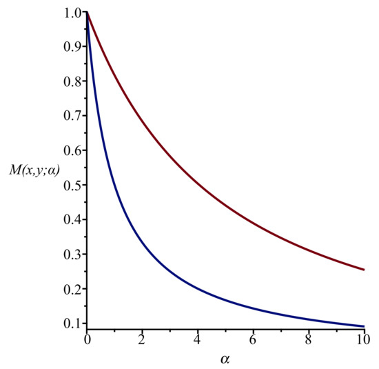
Figure 1. Functions $M_0\left(\alpha \right)$ (below) and $M(x,y;\alpha )$ for $\alpha$ in the interval $(0,10)$, when $\lambda =1$, $k_1=0$, $k_2=1$ and $y-x=0.5$.

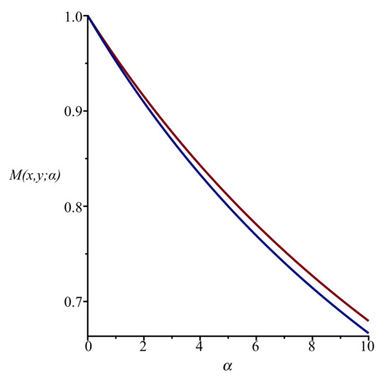
Figure 2. Functions $M_0\left(\alpha \right)$ (below) and $M(x,y;\alpha )$ for $\alpha$ in the interval $(0,10)$, when $\lambda =20$, $k_1=0$, $k_2=1$ and $y-x=0.5$.

Next, the function $m(x,y)=E\left[T\right(x,y\left)\right]$ satisfies the PDE (see Equation (20))

$$-1=\frac{1}{2}{m}_{yy}(x,y)+(y-x)m_x(x,y)-\lambda m(x,y),$$

(65)

subject to $m(x,y)=0$ if $y-x=k_1$ or $k_2$. Setting $m(x,y)=n\left(r\right)$, we obtain the ODE

$$-1=\frac{1}{2}n″\left(r\right)-r{N}^{\prime }\left(r\right)-\lambda N\left(r\right),$$

(66)

with $n\left(k_i\right)=0$, for $i=1,2$. We find that

$$n\left(r\right)=c_{1}rM\left(\frac{1+\lambda }{2},\frac{3}{2},r^2\right)+c_{2}rU\left(\frac{1+\lambda }{2},\frac{3}{2},r^2\right)+\frac{1}{\alpha }.$$

(67)

The particular solution that satisfies the boundary conditions $n\left(0\right)=n\left(1\right)=0$ is presented in Figure 3.

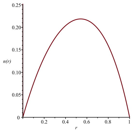
Figure 3. Function $n\left(r\right)$ for $0\le r\le 1$, when $\lambda =1$, $k_1=0$ and $k_2=1$.

Finally, let

$$p(x,y)=P[Y\left(T\right)-X\left(T\right)=k_1\mid X\left(0\right)=x,Y\left(0\right)=y].$$

(68)

This function is a solution of the PDE

$$0=\frac{1}{2}{p}_{yy}(x,y)+(y-x)p_x(x,y)+\lambda [p_0-p(x,y)].$$

(69)

Assuming that $p(x,y)=q\left(r\right)$, we obtain the ODE

$$0=\frac{1}{2}q″\left(r\right)-r{q}^{\prime }\left(r\right)+\lambda [p_0-q\left(r\right)],$$

(70)

whose general solution is

$$q\left(r\right)=c_{1}rM\left(\frac{1+\lambda }{2},\frac{3}{2},r^2\right)+c_{2}rU\left(\frac{1+\lambda }{2},\frac{3}{2},r^2\right)+p_0.$$

(71)

The solution that satisfies the boundary conditions $q\left(0\right)=1$ and $q\left(1\right)=0$ is shown in Figure 4, when $\lambda =1$ and $p_0=1/2$.

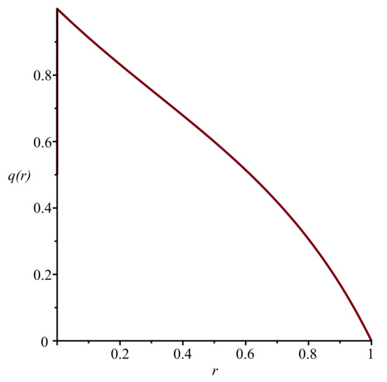
Figure 4. Function $q\left(r\right)$ for $0\le r\le 1$, when $\lambda =1$, $k_1=0$, $k_2=1$ and $p_0=1/2$.

To conclude this section, we will try to find the optimal control of the two-dimensional process $(X_u\left(t\right),Y_u\left(t\right))$ defined by

$$\begin{array}{ccc}\hfill X_u\left(t\right)& =& X_u\left(0\right)+{\int }_0^t[Y_u\left(s\right)-X_u\left(s\right)]\mathrm{d}s,\hfill \end{array}$$

(72)

$$\begin{array}{ccc}\hfill Y_u\left(t\right)& =& Y_u\left(0\right)+{\int }_0^{t}bu[X_u\left(s\right),Y_u\left(s\right)]\mathrm{d}s+B\left(t\right)+\sum _{n=1}^{N\left(t\right)}{Z}_n.\hfill \end{array}$$

(73)

To do so, we must solve the non-linear second-order PDE

$$0=\theta -\frac{1}{2}\frac{b^2}{q}{F}_y^2(x,y)+(y-x)F_x(x,y)+\frac{1}{2}{F}_{yy}(x,y)-\lambda F(x,y),$$

(74)

subject to $F(x,y)=0$ if $y-x=k_1$ or $k_2$.

As above, we make use of the method of similarity solutions. We look for a solution of the form $F(x,y)=G(r=y-x)$. Equation (74) becomes

$$0=\theta -\frac{1}{2}\frac{b^2}{q}{\left[G^{\prime }\left(r\right)\right]}^2-r{G}^{\prime }\left(r\right)+\frac{1}{2}{G}^{\prime \prime }\left(r\right)-\lambda G\left(r\right).$$

(75)

If $\lambda =0$, Maple is able to obtain the general solution of the preceding equation:

$$G\left(r\right)=-\frac{q}{b^2}\left[w^2+ln({\Delta }_1/{\Delta }_2)\right],$$

(76)

where

$${\Delta }_1:=b^2\left[c_{1}M\left(\frac{b^2\theta +q}{2q},\frac{3}{2},r^2\right)+c_{2}U\left(\frac{b^2\theta +q}{2q},\frac{3}{2},r^2\right)\right]$$

(77)

and

$$\begin{array}{ccc}\hfill {\Delta }_2& :=& (b^2\theta -2q)U\left(\frac{b^2\theta +q}{2q},\frac{3}{2},r^2\right)M\left(\frac{b^2\theta -q}{2q},\frac{3}{2},r^2\right)\hfill \\ & & -2qM\left(\frac{b^2\theta +q}{2q},\frac{3}{2},r^2\right)U\left(\frac{b^2\theta -q}{2q},\frac{3}{2},r^2\right).\hfill \end{array}$$

(78)

The constants $c_1$ and $c_2$ are determined by making use of the boundary conditions $G\left(k_1\right)=G\left(k_2\right)=0$.

When $\lambda >0$, Maple and Mathematica are unable to provide an analytical expression for the solution of Equation (75). It is, however, not difficult to obtain a numerical solution for any choice of the parameters. For instance, if we choose $b=q=\theta =\lambda =1$, $k_1=1$ and $k_2=2$, we obtain the function $G\left(r\right)$, as shown in Figure 5, together with the function obtained when $\lambda =0$. Finally, in Figure 6, we present the corresponding optimal controls.

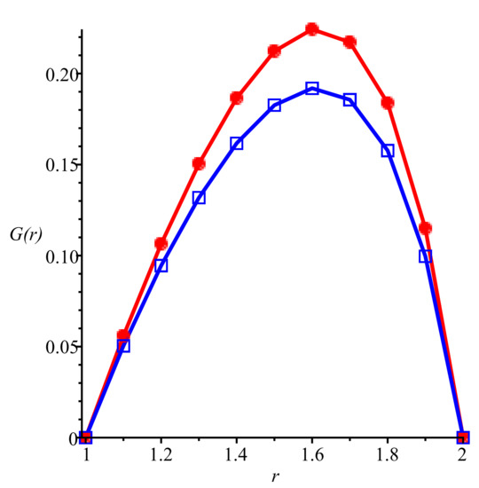
Figure 5. Function $G\left(r\right)$ for $1\le r\le 2$, when $b=q=\theta =1$, $k_1=1$, $k_2=2$, and $\lambda =1$ (with the squares) and $\lambda =0$ (with the circles).

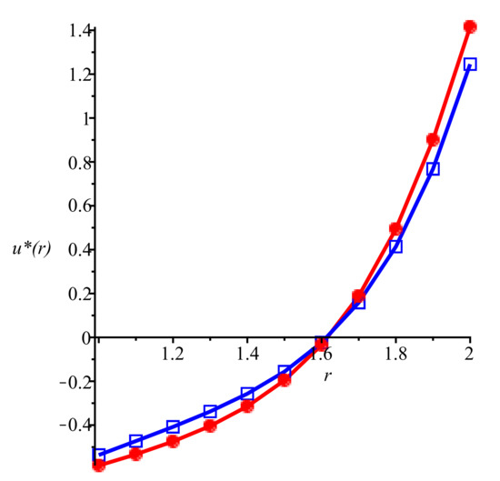
Figure 6. Optimal control in the interval $[1,2]$ when $b=q=\theta =1$, $k_1=1$, $k_2=2$, and $\lambda =1$ (with the squares) and $\lambda =0$ (with the circles).

5. Conclusions

In this paper, we have considered degenerate two-dimensional jump-diffusion processes, defined in such a way that the first component of the vector $\left(X\right(t),Y(t\left)\right)$ is a strictly increasing or decreasing function with respect to time. This kind of process is more realistic than a one-dimensional diffusion or jump-diffusion process in many applications, especially when $X\left(t\right)$ represents the age or wear of a certain device. We could generalize the model by incorporating more than one diffusion process $Y\left(t\right)$. The diffusion processes could model the various variables that influence $X\left(t\right)$. For example, in the case of wear, important factors to consider are temperature, speed of use, etc.

In Section 2, we obtained equations for functions defined in terms of a first-passage time for the processes $\left(X\right(t),Y(t\left)\right)$. Moreover, we treated an optimal control problem for these processes in Section 3. Finally, a particular problem was solved explicitly in Section 4.

As mentioned in Section 1, there are few first-passage problems for one-dimensional jump-diffusion processes that have been solved exactly and explicitly so far. Here, we were able to find exact analytical expressions for quantities defined in terms of a first-passage time for a (degenerate) two-dimensional jump-diffusion process. Furthermore, in Section 2, we saw that the processes considered in this paper could serve as models in real-life applications, such as the remaining amount of deterioration that a given device can undergo before it needs to be repaired or replaced.

In general, to solve this type of problem, it is necessary to find the solution of an integro-differential equation with partial derivatives. We considered the case when the process leaves the continuation region at the latest when the first event of the Poisson process occurs. In this case, the equation to be solved becomes a partial differential equation. Using the method of similarity solutions, it is sometimes possible to reduce this PDE to an ODE. It should also be possible to find a numerical solution to any particular problem.

As a follow-up to this work, we would like to find exact analytical solutions to problems where the equations to be solved are integro-differential equations; for example, by trying to transform the integro-differential equations into differential equations.

References

- Höpfner, R. On a set of data for the membrane potential in a neuron. Math. Biosci. 2007, 207, 275–301. [Google Scholar] [CrossRef] [PubMed]
- Jahn, P.; Berg, R.W.; Hounsgaard, J.; Ditlevsen, S. Motoneuron membrane potentials follow a time inhomogeneous jump diffusion process. J. Comput. Neurosci. 2011, 31, 563–579. [Google Scholar] [CrossRef] [PubMed]
- Melanson, A.; Longtin, A. Data-driven inference for stationary jump-diffusion processes with application to membrane voltage fluctuations in pyramidal neurons. J. Math. Neurosci. 2019, 9, 30. [Google Scholar] [CrossRef] [PubMed]
- Lefebvre, M. A first-passage problem for exponential integrated diffusion processes. J. Stoch. Anal. 2022, 3, 2. [Google Scholar] [CrossRef]
- Lachal, A. L’intégrale du mouvement brownien. J. Appl. Probab. 1993, 30, 17–27. [Google Scholar] [CrossRef]
- Makasu, C. Exit probability for an integrated geometric Brownian motion. Stat. Probab. Lett. 2009, 79, 1363–1365. [Google Scholar] [CrossRef]
- Metzler, A. The Laplace transform of hitting times of integrated geometric Brownian motion. J. Appl. Probab. 2013, 50, 295–299. [Google Scholar] [CrossRef]
- Caravelli, F.; Mansour, T.; Sindoni, L.; Severini, S. On moments of the integrated exponential Brownian motion. Eur. Phys. J. Plus 2008, 131, 245. [Google Scholar] [CrossRef]
- Levy, E. On the moments of the integrated geometric Brownian motion. J. Comput. Appl. Math. 2018, 342, 263–273. [Google Scholar] [CrossRef]
- Cox, D.R.; Miller, H.D. The Theory of Stochastic Processes; Methuen: London, UK, 1965. [Google Scholar]
- Kou, S.G.; Wang, H. First passage times of a jump diffusion process. Adv. Appl. Probab. 2003, 35, 504–531. [Google Scholar] [CrossRef]
- Chen, Y.-T.; Sheu, Y.-C.; Chang, M.-C. A note on first passage functionals for hyper-exponential jump-diffusion processes. Electron. Commun. Probab. 2013, 18, 8. [Google Scholar] [CrossRef]
- Yin, C.; Wen, Y.; Zong, Z.; Shen, Y. The first passage time problem for mixed-exponential jump processes with applications in insurance and finance. Abstr. Appl. Anal. 2014, 2014, 571724. [Google Scholar] [CrossRef]
- Karnaukh, I. Exit problems for Kou’s process in a Markovian environment. Theory Stoch. Process. 2020, 25, 37–60. [Google Scholar] [CrossRef]
- Lefebvre, M. Exit problems for jump-diffusion processes with uniform jumps. J. Stoch. Anal. 2020, 1, 5. [Google Scholar] [CrossRef]
- Abundo, M. On first-passage times for one-dimensional jump-diffusion processes. Probab. Math. Stat. 2020, 20, 399–423. [Google Scholar]
- Belkaid, A.; Utzet, F. Efficient computation of first passage times in Kou’s jump-diffusion model. Methodol. Comput. Appl. Probab. 2017, 19, 957–971. [Google Scholar] [CrossRef]
- Di Crescenzo, A.; Di Nardo, E.; Ricciardi, L.M. On certain bounds for first-crossing-time probabilities of a jump-diffusion process. Sci. Math. Jpn. 2006, 64, 449–460. [Google Scholar]
- Fernández, L.; Hieber, P.; Scherer, M. Double-barrier first-passage times of jump-diffusion processes. Monte Carlo Methods Appl. 2013, 19, 107–141. [Google Scholar] [CrossRef]
- D’Onofrio, G.; Lanteri, A. Approximating the first passage time density of diffusion processes with state-dependent jumps. Fractal Fract. 2023, 7, 30. [Google Scholar] [CrossRef]
- Lefebvre, M. Exact solutions to optimal control problems for Wiener processes with exponential jumps. J. Stoch. Anal. 2021, 2, 1. [Google Scholar] [CrossRef]
- Rishel, R. Controlled wear process: Modeling optimal control. IEEE Trans. Autom. Control 1991, 36, 1100–1102. [Google Scholar] [CrossRef]
- Whittle, P. Optimization over Time; Wiley: Chichester, UK, 1982; Volume 1. [Google Scholar]
- Whittle, P. Risk-Sensitive Optimal Control; Wiley: Chichester, UK, 1990. [Google Scholar]
Disclaimer/Publisher’s Note: The statements, opinions and data contained in all publications are solely those of the individual author(s) and contributor(s) and not of MDPI and/or the editor(s). MDPI and/or the editor(s) disclaim responsibility for any injury to people or property resulting from any ideas, methods, instructions or products referred to in the content. |
© 2023 by the author. Licensee MDPI, Basel, Switzerland. This article is an open access article distributed under the terms and conditions of the Creative Commons Attribution (CC BY) license (https://creativecommons.org/licenses/by/4.0/).