

Bifurcation and Analytical Solutions of the Space-Fractional Stochastic Schrödinger Equation with White Noise

Abstract
:1. Introduction
2. Mathematical Analysis
3. Bifurcation of the Phase Portraits
- 1.
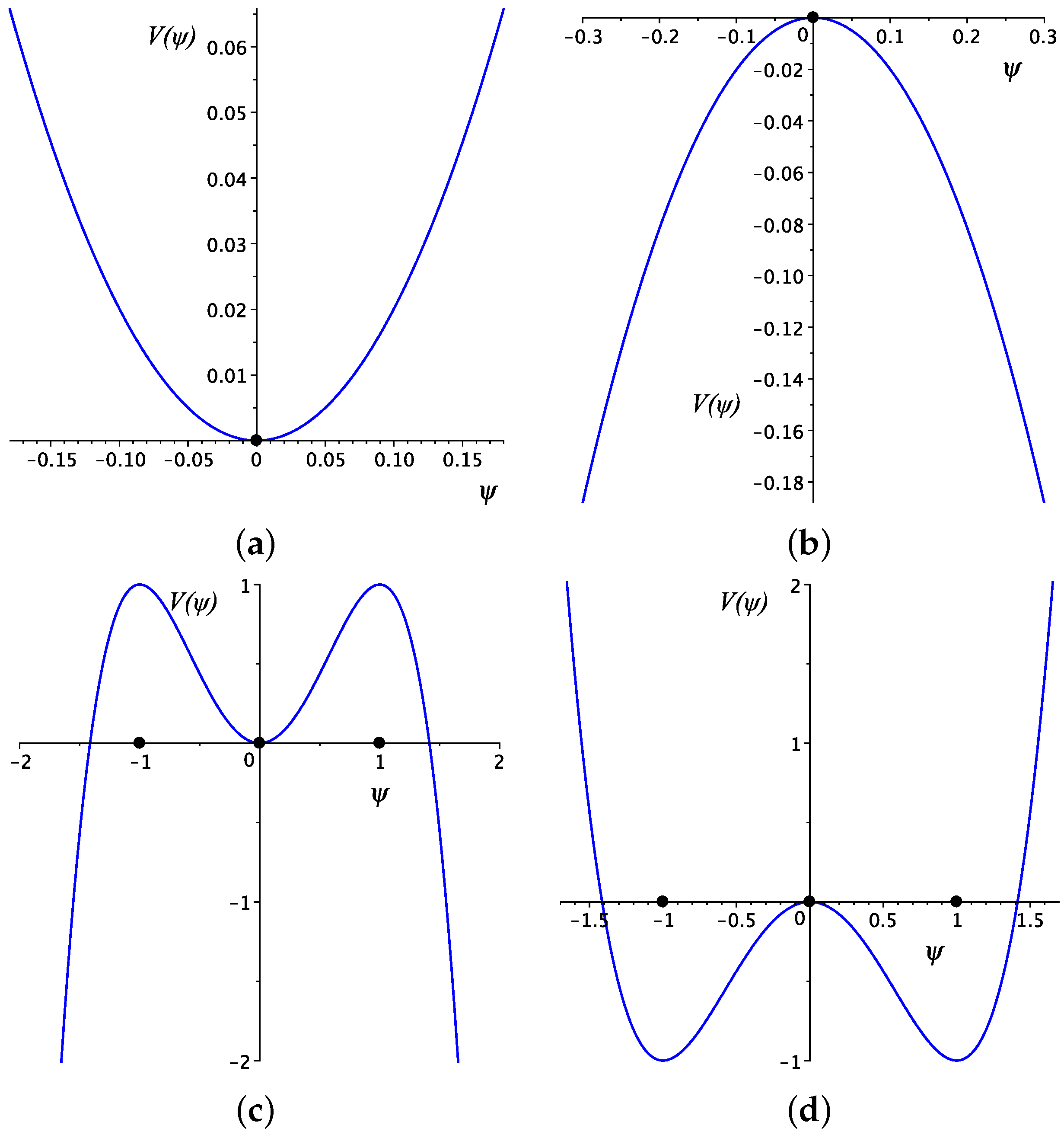
- If , then is the unique equilibrium point for system (14), and a local minimum for the potential function (16) as illustrated in Figure 1a. Hence, it is a center for the Hamiltonian system (14).
- 2.
- If , then system (14) has as the unique equilibrium, and a local maximum for the potential function (16), as illustrated in Figure 1b. Hence, it is a saddle point for the Hamiltonian system (14).
- 3.
- If , then system (14) has three equilibrium points . As illustrated in Figure 1, is local minimum for the potential (16) while are local maxima points for the potential (1). Hence, is a center and are saddle points for the Hamiltonian system (14).
- 4.
- If , then there are three equilibrium points for the system (14) with a saddle and centers.
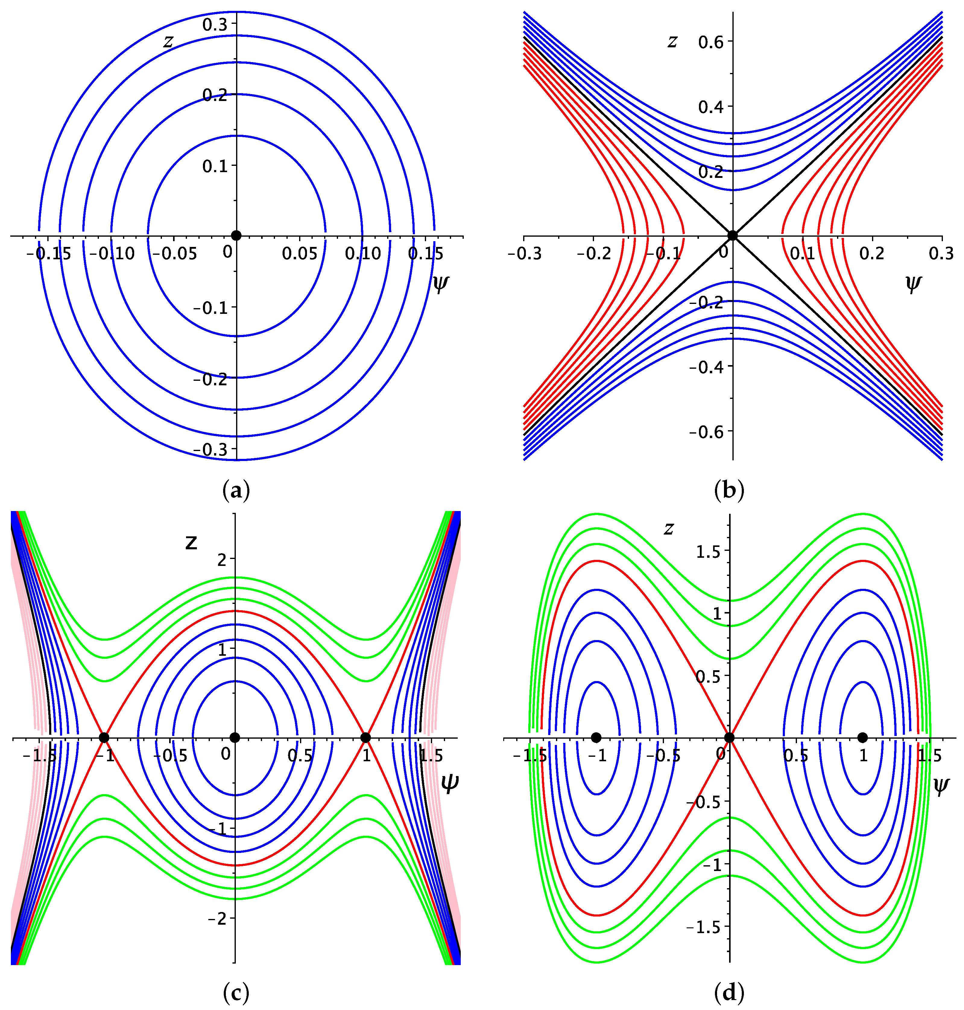
- For , the phase portrait consists of a family of bounded periodic orbits about the center equilibrium point , as shown in Figure 2a. These orbits indicate the existence of periodic wave solutions for the system (14).
- For , the phase orbits for the system (14) are unbounded, as shown in Figure 2b, where these orbits are color-coded with shown in black, in blue, and in red. These orbits indicate the existence of unbounded wave solutions.
- For , the phase portrait for the system (14) is shown in Figure 2c. There is a family of unbound orbits , shown in green. For , we obtain a heteroclinic orbit, shown in red, connecting the two saddle points with two unbounded extensions. The heteroclinic orbit indicate the existence of kink (or anti-kink) wave solution and unbounded wave solutions. For , there are three families of orbits shown in blue. One is periodic and lies inside the heteroclinic orbit while the others are unbounded. Finally, for , we have two unbounded family of orbits in pink while, when , there are two unbounded orbits in black, in addition to the equilibrium point .
- For , all the orbits of the Hamilton system (14) are bounded, as shown in Figure 2d. There are two periodic families of bounded orbits, shown in blue . These families are contained in the homoclinic orbit , shown in red, which provides a solitary solution. For , there is a family of super periodic orbits, shown in green. These indicate the existence of the super periodic wave solution.
4. Traveling Wave Solutions
- 1.
- periodic solutions if ,
- 2.
- kink (anti-kink) solution if ,
- 3.
- solitary solution if .
4.1. Periodic Solutions
- 1.
- For and , system (14) has a bounded family of periodic orbits, shown in Figure 2a. Each orbit of this family intersects axis at two points, indicating that has two real roots, which denote . Thus, we can write . The interval of the real solution is . Integrating both sides of Equation (12) along this interval, we obtainThus, we can obtain a bi-periodic wave solution, given byThis gives us a solution of Equation (1), with the the formWe note that solution (24) is a new solution for Equation (1).
- 2.
- For and , system (14) has two types of orbits, shown in blue in Figure 2c one periodic and the other unbounded. An orbit of this family crosses the axis in four points; hence, has four real roots, , where , i.e., . The interval of real solutions is . We will only consider , avoiding the investigation of the unbounded solutions at present. Integrating both sides of Equation (12) givesThis equation givesThus, Equation (1) has a novel solution in the form
- 3.
- If , system (14) has two families of periodic orbits, as shown in blue and green in Figure 2d. These families are:
- For , the system (14) has a family of periodic orbits, shown in blue, each of which cuts the axis at four points, showing that has four real roots, denoted as , where . Thus, we can write . The interval of the real solution is , with corresponding to a periodic family on the left of the oval homoclinic orbit, shown in red, and to a periodic family lying to the right of the oval homoclinic orbit. We will only consider the one on the left, as the calculation for the other is similar. The integration of both sides of Equation (12) along the interval showsFrom which it follows thatTherefore, Equation (1) has the solutionSolution (33) is a new solution for Equation (1).
- For , there is a family of super-periodic orbits, shown in green. A member of this family intersects axis at two points, and so has two real zeros, namely, , and two purely imaginary roots . Thus, . The interval of the real solution is . By integrating both sides of Equation (12), we obtainFrom the above equation, we can obtainTherefore, Equation (12) has the solution
The last solution is a novel solution for Equation (1).
4.2. Kink(Anti-Kink) Solutions
4.3. Solitary Solution
- 1.
- In the absence of the noise , the stochastic fractional-space partial differential Equation (1) becomes a fractional-space partial differential equation. Thus, setting in the solutions (24), (27), (33), (32), (36), and (38), we obtain new solutions for the latter equation.
- 2.
- Equation (1) approaches the stochastic partial differential equation when the fractional-order derivative α approaches one. Thus, when , the solutions (24), (27), (33), (32), (36), and (38) converge to new solutions for the stochastic equation.
- 3.
- When and , Equation (1) becomes a classical partial differential equation. Thus, the solutions (24), (27), (33), and (32) yield new solutions to the classical equations.
- 1.
- The periodic family of orbits around the center point O shown in Figure 2a degenerates to the center point when , which means that when . Thus, the solution (24) approaches , which are the coordinates of the equilibrium point O.
- 2.
- The periodic family of orbits around the center point O shown in blue in Figure 2c degenerates into:
- The center point O when , which means that . Thus, the solution (27) approaches , the coordinates of the equilibrium point O.
- The hetroclinic orbit shown in red in Figure 2c when and then and . Hence, the solution (27) approaches the solution (36).
- 3.
- The periodic family of orbits shown in blue in Figure 2d will approach the homoclinic orbit, shown in red, when and therefore, . Thus, the solution (33) approaches the solution (38).
- 4.
- The family of super-periodic orbits in green in Figure 2d will approach the two homoclinic orbits in red when ; therefore, . Hence, the solution (32) will approach the solution (38).
5. Graphic Representation
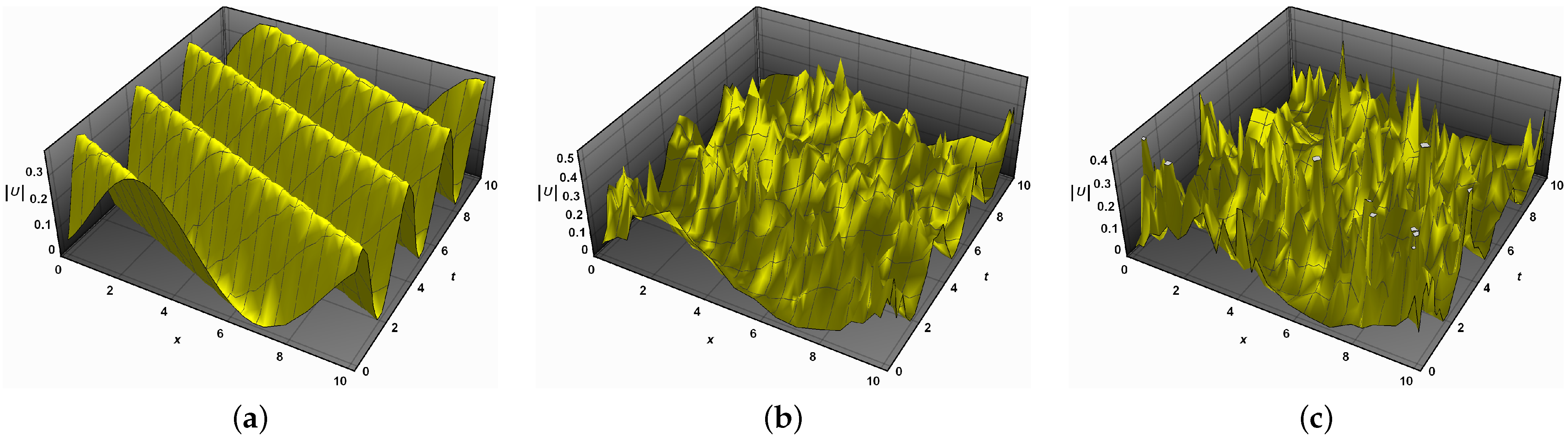
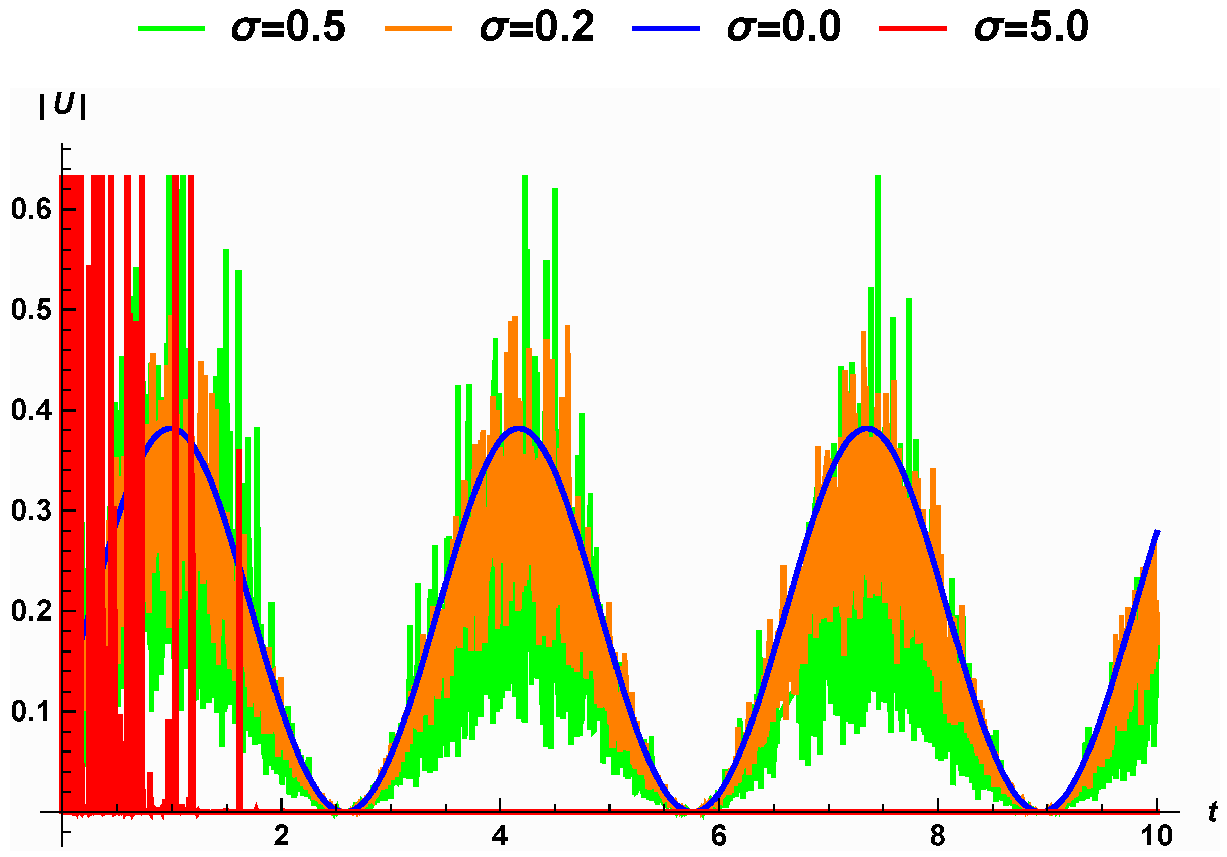
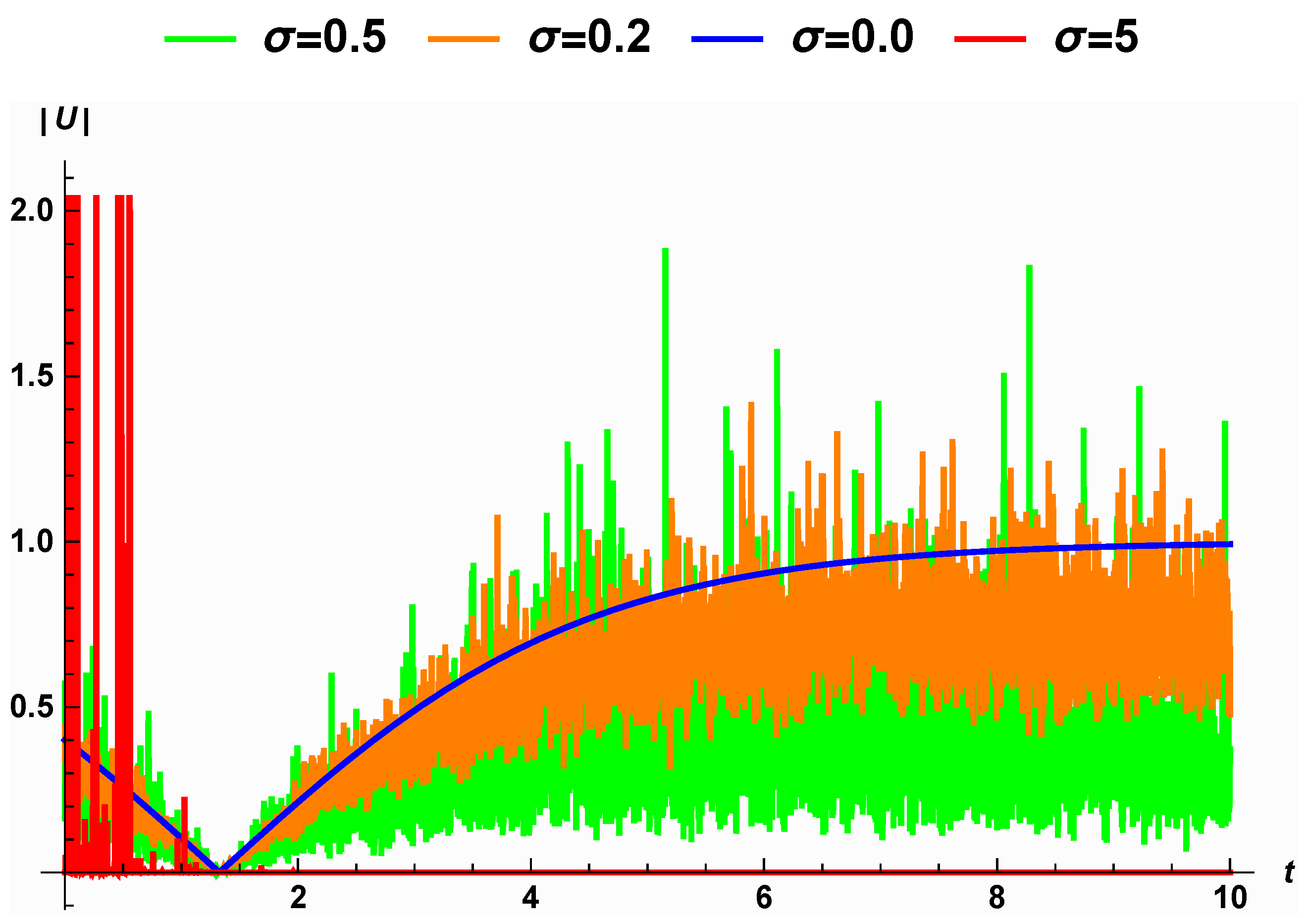
- The effect of the noise on the solution (24) for the noise values , and is shown in Figure 3. Figure 3a shows the solution of (24), which is periodic in the absence of the noise (). The introduction of noise generates disturbances in the solution, as shown in Figure 3b,c. In Figure 4, we present a 2D representation of the solution of (24). When , the solution, shown in blue, is periodic. Increasing the noise causes increasing disturbances to the periodic solution. Additionally, the 2D representation of the surface, shown in red in Figure 4, shows that when the noise increases, the surface becomes significantly flatter after minor transit patterns.
- The classical version of Equation (1) with zero noise and integer fractional order has a kink solution (36), as shown in Figure 5a, and its 2D representation is shown in blue in Figure 6. Figure 5b,c show the changes in the shape of the solution (36) due to small noise values , and their 2D representations clarify these changes. For larger noise values, the surface that characterizes the wave solution (36) become significantly flat, as shown in red by Figure 6.
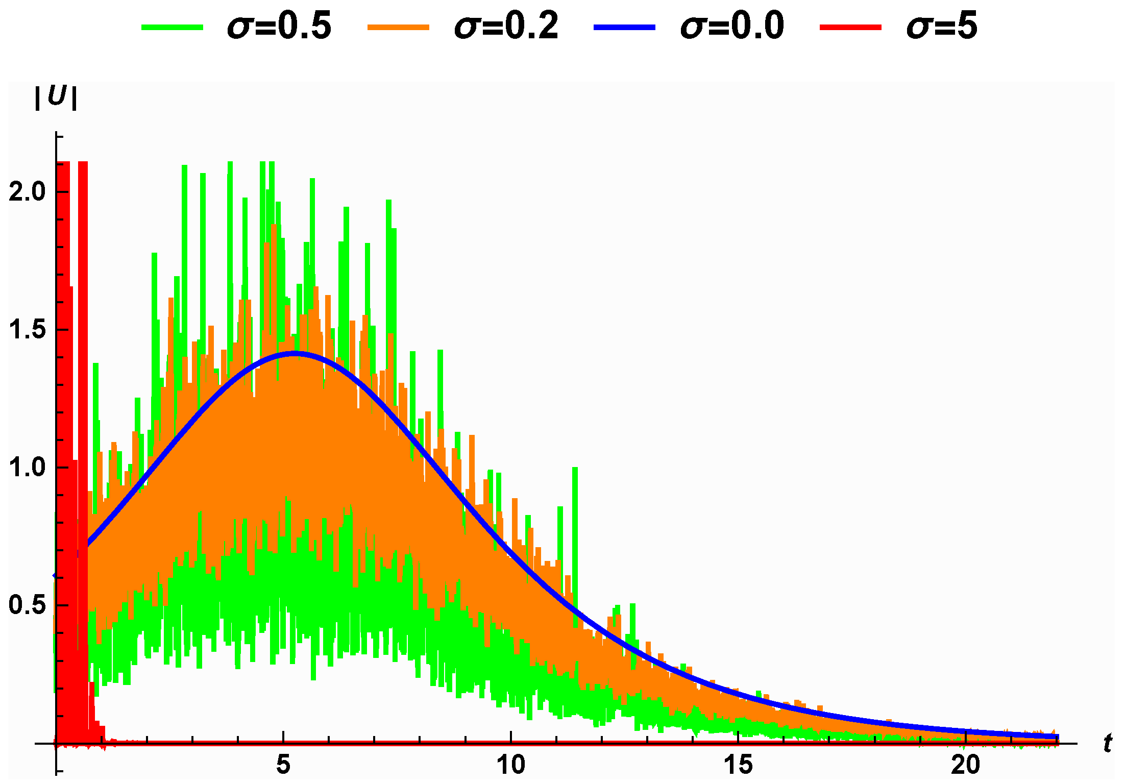
- In the absence of noise and fractional order, , Equation (1) has one soliton solution, as shown in Figure 7a, with its 2D representation appearing in blue in Figure 8. For low noise values and , the surface representing the solution (38) has some disturbances, which increasing with increases in noise , as shown in Figure 7b,c. This is also shown in Figure 8, presenting a 2D representation of the solution. For large noise values , the surface representing the solution (38) becomes flat, as shown in Figure 8 in red. Thus, it is clear that the stochastic Wiener process influences the solution (38) of Equation (1) and also stabilizes the solutions at around zero.
6. Discussion
Funding
Data Availability Statement
Acknowledgments
Conflicts of Interest
Appendix A. Conformable Derivatives
- 1.
- ,
- 2.
- , ,
- 3.
- .
- 4.
- 5.
- If f is differentiable at t then .
- 1.
- ;
- 2.
- is a continuous function for ;
- 3.
- For and are independent;
- 4.
- has a normal distribution with mean zero and variance .
References
- Biswas, A. Stochastic perturbation of optical solitons in Schrödinger–Hirota equation. Opt. Commun. 2004, 239, 461–466. [Google Scholar] [CrossRef]
- Khan, S. Stochastic perturbation of optical solitons having generalized anti-cubic non-linearity with band pass filters and multi-photon absorption. Optik 2020, 200, 163405. [Google Scholar] [CrossRef]
- Ulutas, E. Travelling wave and optical soliton solutions of the Wick-type stochastic NLSE with conformable derivatives. Chaos Solitons Fractals 2021, 148, 111052. [Google Scholar] [CrossRef]
- Ghany, H.A.; Mohammed, M.S. White noise functional solutions for Wick-type stochastic fractional KdV-Burgers-Kuramoto equations. Chin. J. Phys. 2012, 50, 619–627. [Google Scholar]
- Li, Z.; Li, P.; Han, T. White Noise Functional Solutions for Wick-Type Stochastic Fractional Mixed KdV-mKdV Equation Using Extended-Expansion Method. Adv. Math. Phys. 2021, 2021, 9729905. [Google Scholar] [CrossRef]
- Kim, H.; Sakthivel, R.; Debbouche, A.; Torres, D.F. Traveling wave solutions of some important Wick-type fractional stochastic nonlinear partial differential equations. Chaos Solitons Fractals 2020, 131, 109542. [Google Scholar] [CrossRef]
- Han, T.; Li, Z.; Shi, K.; Wu, G.C. Bifurcation and traveling wave solutions of stochastic Manakov model with multiplicative white noise in birefringent fibers. Chaos Solitons Fractals 2022, 163, 112548. [Google Scholar] [CrossRef]
- Weinan, E.; Li, X.; Vanden-Eijnden, E. Some recent progress in multi scale modeling. In Multiscale Modelling and Simulation; Springer: Berlin/Heidelberg, Germany, 2004; pp. 3–21. [Google Scholar]
- Imkeller, P.; Monahan, A.H. Conceptual stochastic climate models. Stochastics Dyn. 2002, 2, 311–326. [Google Scholar] [CrossRef]
- Alhamud, M.; Elbrolosy, M.; Elmandouh, A. New Analytical Solutions for Time-Fractional Stochastic (3+ 1)-Dimensional Equations for Fluids with Gas Bubbles and Hydrodynamics. Fractal Fract. 2023, 7, 16. [Google Scholar] [CrossRef]
- Secer, A. Stochastic optical solitons with multiplicative white noise via Itô calculus. Optik 2022, 268, 169831. [Google Scholar] [CrossRef]
- Zayed, E.M.; Shohib, R.M.; Alngar, M.E.; Biswas, A.; Moraru, L.; Khan, S.; Belic, M.R. Dispersive optical solitons with Schrödinger–Hirota model having multiplicative white noise via Itô calculus. Phys. Lett. A 2022, 445, 128268. [Google Scholar] [CrossRef]
- Tarasov, V.E. Fractional Dynamics: Applications of Fractional Calculus to Dynamics of Particles, Fields and Media; Springer Science: New York, NY, USA, 2011. [Google Scholar]
- El-Nabulsi, R.A. Path integral formulation of fractionally perturbed Lagrangian oscillators on fractal. J. Stat. Phys. 2018, 172, 1617–1640. [Google Scholar] [CrossRef]
- Dong, J.; Xu, M. Space–time fractional Schrödinger equation with time-independent potentials. J. Math. Anal. Appl. 2008, 344, 1005–1017. [Google Scholar] [CrossRef]
- Bayın, S.S. On the consistency of the solutions of the space fractional Schrödinger equation. J. Math. Phys. 2012, 53, 042105. [Google Scholar] [CrossRef]
- Abu Arqub, O. Application of residual power series method for the solution of time-fractional Schrödinger equations in one-dimensional space. Fundam. Inform. 2019, 166, 87–110. [Google Scholar] [CrossRef]
- Wang, F.; Khan, M.N.; Ahmad, I.; Ahmad, H.; Abu-Zinadah, H.; Chu, Y. Numerical Solution of Traveling Waves in Chemical Kinetics: Time-Fractional Fishers Equations. Fractional 2022, 30, 2240051. [Google Scholar]
- Jia, H.X. Solitons in PT symmetric Manakov system. Optik 2021, 230, 166223. [Google Scholar] [CrossRef]
- Ramakrishnan, R.; Stalin, S.; Lakshmanan, M. Nondegenerate solitons and their collisions in Manakov systems. Phys. Rev. E 2020, 102, 042212. [Google Scholar] [CrossRef]
- Ma, W.X.; Batwa, S. A binary Darboux transformation for multicomponent NLS equations and their reductions. Anal. Math. Phys. 2021, 11, 1–12. [Google Scholar] [CrossRef]
- Han, T.; Li, Z.; Yuan, J. Optical solitons and single traveling wave solutions of Biswas-Arshed equation in birefringent fibers with the beta-time derivative. AIMS Math. 2022, 7, 15282–15297. [Google Scholar] [CrossRef]
- Cheemaa, N.; Chen, S.; Seadawy, A.R. Propagation of isolated waves of coupled nonlinear (2+ 1)-dimensional Maccari system in plasma physics. Results Phys. 2020, 17, 102987. [Google Scholar] [CrossRef]
- Seadawy, A.R.; Iqbal, M.; Lu, D. Propagation of kink and anti-kink wave solitons for the nonlinear damped modified Korteweg–de Vries equation arising in ion-acoustic wave in an unmagnetized collisional dusty plasma. Phys. A Stat. Mech. Its Appl. 2020, 544, 123560. [Google Scholar] [CrossRef]
- El Achab, A. Constructing of exact solutions to the nonlinear Schrödinger equation (NLSE) with power-law nonlinearity by the Weierstrass elliptic function method. Optik 2016, 127, 1229–1232. [Google Scholar] [CrossRef]
- Fan, E.; Zhang, J. Applications of the Jacobi elliptic function method to special-type nonlinear equations. Phys. Lett. A 2002, 305, 383–392. [Google Scholar] [CrossRef]
- Kumar, S.; Dhiman, S.K.; Baleanu, D.; Osman, M.S.; Wazwaz, A.M. Lie symmetries, closed-form solutions, and various dynamical profiles of solitons for the variable coefficient (2+ 1)-dimensional KP equations. Symmetry 2022, 14, 597. [Google Scholar] [CrossRef]
- Jiang, Z.; Zhang, Z.G.; Li, J.J.; Yang, H.W. Analysis of Lie symmetries with conservation laws and solutions of generalized (4+ 1)-dimensional time-fractional Fokas equation. Fractal Fract. 2022, 6, 108. [Google Scholar] [CrossRef]
- Tanwar, D.V.; Ray, A.K.; Chauhan, A. Lie Symmetries and Dynamical Behavior of Soliton Solutions of KP-BBM Equation. Qual. Theory Dyn. Syst. 2022, 21, 1–14. [Google Scholar] [CrossRef]
- Elbrolosy, M.E.; Elmandouh, A.A. Dynamical behaviour of conformable time-fractional coupled Konno-Oono equation in magnetic field. Math. Probl. Eng. 2022, 2022, 3157217. [Google Scholar]
- Elmandouh, A.A.; Elbrolosy, M.E. New traveling wave solutions for Gilson–Pickering equation in plasma via bifurcation analysis and direct method. Math. Methods Appl. Sci. 2022. [Google Scholar] [CrossRef]
- Hassan, T.S.; Elmandouh, A.A.; Attiya, A.A.; Khedr, A.Y. Bifurcation Analysis and Exact Wave Solutions for the Double-Chain Model of DNA. J. Math. 2022, 2022, 7188118. [Google Scholar] [CrossRef]
- Elbrolosy, M.E.; Elmandouh, A.A. Dynamical behaviour of nondissipative double dispersive microstrain wave in the microstructured solids. Eur. Phys. J. Plus 2021, 136, 1–20. [Google Scholar] [CrossRef]
- AL Nuwairan, M.A.; Elmandouh, A.A. Qualitative analysis and wave propagation of the nonlinear model for low-pass electrical transmission lines. Phys. Scr. 2021, 96, 095214. [Google Scholar] [CrossRef]
- Wazwaz, A.M. Bright and dark optical solitons for (2+ 1)-dimensional Schrödinger (NLS) equations in the anomalous dispersion regimes and the normal dispersive regimes. Optik 2019, 192, 162948. [Google Scholar] [CrossRef]
- Akinyemi, L.; Şenol, M.; Osman, M.S. Analytical and approximate solutions of nonlinear Schrödinger equation with higher dimension in the anomalous dispersion regime. J. Ocean. Eng. Sci. 2022, 7, 143–154. [Google Scholar] [CrossRef]
- Khalil, R.; Al Horani, M.; Yousef, A.; Sababheh, M. A new definition of fractional derivative. J. Comput. Appl. Math. 2014, 264, 65–70. [Google Scholar] [CrossRef]
- Platen, E.; Bruti-Liberati, N. Numerical Solution of Stochastic Differential Equations with Jumps in Finance; Springer Science & Business Media: Berlin, Germany, 2010; Volume 64. [Google Scholar]
- Kloeden, P.E.; Platen, E. Numerical Solution of Stochastic Differential Equations; Springer: New York, NY, USA, 1995. [Google Scholar]


Disclaimer/Publisher’s Note: The statements, opinions and data contained in all publications are solely those of the individual author(s) and contributor(s) and not of MDPI and/or the editor(s). MDPI and/or the editor(s) disclaim responsibility for any injury to people or property resulting from any ideas, methods, instructions or products referred to in the content. |
© 2023 by the author. Licensee MDPI, Basel, Switzerland. This article is an open access article distributed under the terms and conditions of the Creative Commons Attribution (CC BY) license (https://creativecommons.org/licenses/by/4.0/).
Share and Cite
Al Nuwairan, M. Bifurcation and Analytical Solutions of the Space-Fractional Stochastic Schrödinger Equation with White Noise. Fractal Fract. 2023, 7, 157. https://doi.org/10.3390/fractalfract7020157
Al Nuwairan M. Bifurcation and Analytical Solutions of the Space-Fractional Stochastic Schrödinger Equation with White Noise. Fractal and Fractional. 2023; 7(2):157. https://doi.org/10.3390/fractalfract7020157
Chicago/Turabian StyleAl Nuwairan, Muneerah. 2023. "Bifurcation and Analytical Solutions of the Space-Fractional Stochastic Schrödinger Equation with White Noise" Fractal and Fractional 7, no. 2: 157. https://doi.org/10.3390/fractalfract7020157