Abstract
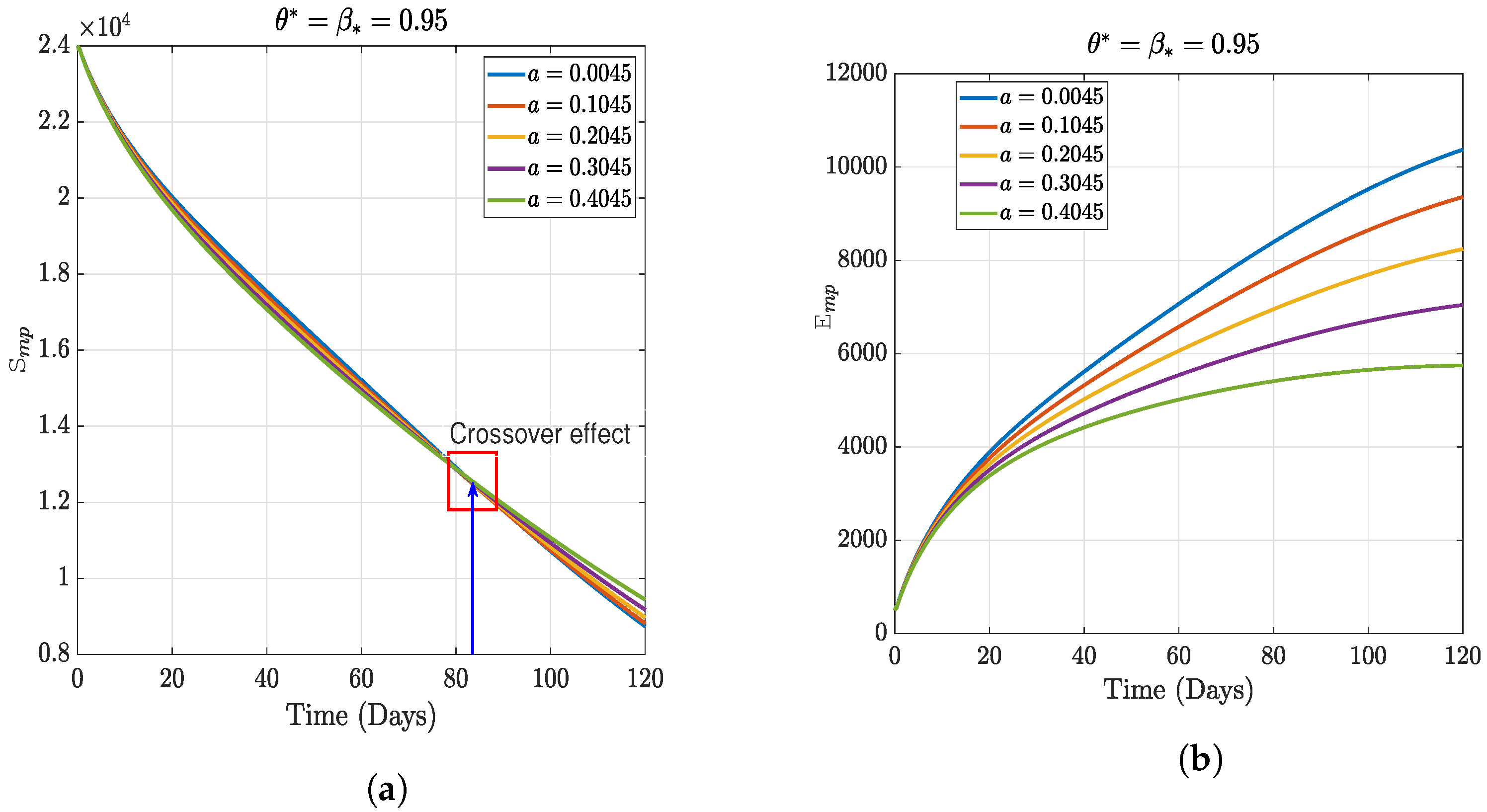
Maize is one of the most extensively produced cereals in the world. The maize streak virus primarily infects maize but can also infect over 80 other grass species. Leafhoppers are the primary vectors of the maize streak virus. When feeding on plants, susceptible vectors can acquire the virus from infected plants, and infected vectors can transmit the virus to susceptible plants. However, because maize is normally patchy and leafhoppers are mobile, leafhoppers will always be foraging for food. Therefore, we want to look at how leafhoppers interact on maize farms using Holling’s Type III functional response in a Caputo fractal-fractional derivative sense. We show that the proposed model has unique positive solutions within a feasible region. We employed the Newton polynomial scheme to numerically simulate the proposed model to illustrate the qualitative results obtained. We also studied the relationship between the state variables and some epidemiological factors captured as model parameters. We observed that the integer-order versions of the model exaggerate the impact of the disease. We also observe that the increase in the leafhopper infestation on maize fields has a devastating effect on the health of maize plants and the subsequent yield. Furthermore, we noticed that varying the conversion rate of the infected leafhopper leads to a crossover effect in the number of healthy maize after 82 days. We also show the dynamics of varying the maize streak virus transmission rates. It indicates that when preventive measures are taken to reduce the transmission rates, it will reduce the low-yielding effect of maize due to the maize streak virus disease.
1. Introduction
In 2016, maize was predicted to be next to yellow rice among cereals in revenue. Regarding the Sustainable Development Goal of eradicating world hunger, plants’ health is crucial as it affects food production. Over 80% of the calories consumed by humans comes from plants. Plants and animals have become more susceptible to disease and pests due to increased travel, unfavorable climate change, and continuous forest encroachment caused by rising populations and urbanization. Close to 40% of the annual global food crop losses are attributable to pests and diseases, so more efforts must be adopted to combat the effect of these pests and diseases [1]. During feeding, susceptible leafhoppers can acquire the virus from infected plants, and infected vectors can, in turn, transmit the virus to susceptible plants. The importance of mathematics in helping us better understand the world around us cannot be overemphasized. Mathematical models are crucial to the development and execution of effective policies for eradicating infectious diseases in plants and animals. Two areas where mathematics is increasingly used are mathematical epidemiology and mathematical ecology, where mathematical tools and techniques are used to study the dynamics of infectious diseases and ecology. Mathematical modeling has been a significant resource for studying the transmission of disease and creating effective prophylactic measures and is effective in aiding a better understanding of infectious disease dynamics and control.
Much research has been conducted using mathematical models to help understand the spread and control of MSVD. Regarding maize disease research, [2] studied the epidemiological compartments of maize plants to explore the most effective control strategies. Using the SEI-SI plant-vector model, the relationship between plants and maize Lethal Necrosis disease (MLND)-vector populations is described by [3]. The contact rates were found to have beneficial effects on the transmission of MLND between maize and MLND vectors and between maize and other plants. Moreover, ref. [4] proposed a susceptible–infected maize-vector differential equation model to analyze the dynamics of MSVD. To investigate the effect of the ambient pathogen concentration on MSVD management, ref. [5] integrated the pathogen compartment into the maize leafhopper model, demonstrating that the removal of infected leafhoppers and the incineration of infected maize plants is a suitable method for controlling the disease. The epidemiological model of Alemneh and colleagues [4] was broadened in [6] to examine the most cost-effective approaches to manage MSVD and made the same findings as [5]. The epidemiological models in [4,5,6] gave in-depth knowledge of the dynamics of MSVD. Still, it is noteworthy that they represent maize plant infection and predation in a multifunctional fashion. Recently, Seidu and colleagues [7] presented a dynamical model of MSVD with the incorporation of the Holling’s Type II and standard incidence to study the best strategies for controlling the spread of MSVD. They noticed that the most cost-effective strategy combines the simultaneous adoption of infection control, predation control, the removal of infected maize plants, and insecticide application.
Finally, the work in [8] included the latent period in the spread of MSVD. We note that much of the research that has been conducted on MSVD modeling does not consider the use of fractal-fractional derivatives. However, researchers are becoming highly involved in using non-integer-scale mathematical modeling of contagious diseases [9]. In epidemiology, fixed-order derivatives can only define classical models, while models with fractional-order derivatives and a fractal order are more effective in representing real-world issues. This superiority of the non-integer models is due to their inherent memory effect, which ensures that current solutions of models rely on all previous solutions and not just the immediate previous solution, as in the case of integer-order models. A new non-integer differentiation concept is presented in [10,11], where the operator has two orders: a fractional order and a fractal dimension (order). Thus, to show the dynamism of this new concept, the work in [12] used fractal-fractional derivatives and integrals to study and forecast the dynamic behavior of some attractors. Moreover, the work in [13] investigated novel numerical approximations for the Chua attractor using fractional and fractal-fractional operators. Due to the new insight, the fractal-fractional investigation brings the following works [14,15,16,17,18,19,20,21,22,23], giving various valuable epidemiological importance to the concept of fractal-fractional modeling on numerous diseases, including COVID-19. Sinan et al. [24] studied the fractional model of malaria disease with treatment and insecticides and observed that the utilization of bed nets and insecticides could drastically cut down on the transmission of malaria. However, the effect of medication and treatment on infection regulation is relatively less significant. Ahmad et al. [25] studied the dynamics and sensitivity analysis of pine wilt disease with asymptomatic carriers via the fractal-fractional differential operator of the Mittag-Leffler kernel and found that eliminating beetles might significantly lower the infection. The work in [26] used a fractal-fractional model to study the sensitivity analysis of COVID-19, which included both quarantine and vaccination. The use of fractional and fractal derivatives to model maize streak disease dynamics has not been considered to the best of our knowledge. Therefore, this work is the first to study the effect of maize streak disease using the Caputo fractal-fractional derivative. This study has been conducted because the fractal-fractional derivative can help capture the repeated and memory aspects of natural phenomena. Moreover, the potential outcome of the further spread of the maize streak virus can be captured by the Caputo fractal-fractional derivative. The rest of this paper is arranged as follows: Some fundamental definitions and preliminary information are provided in Section 2. We present our proposed model in integer and fractal-fractional forms in Section 3. Section 4 presents the analysis of the Caputo fractal-fractional model. We present the numerical results of the Caputo fractal-fractional model in Section 5. Finally, Section 6 provides this study’s conclusion.
2. Preliminaries
In this part, the general definitions concerning the fractal-fractional Caputo are presented.
Definition 1
([10,27]). Given a continuous interval , and assuming that is differentiable on the fractal dimension interval . Following that, the Caputo fractal-fractional differential operator of of order is provided by
with the following derivative:
If , then the Caputo fractal-fractional derivative becomes the -Riemann–Liouville derivative .
Definition 2
([10,27]). Suppose that is uninterrupted on the open interval . Then, the fractal-fractional integral of of the Caputo operator is written as
Let be categorized under the umbrella of nondecreasing mappings with and
Definition 3
([27,28]). Suppose and , with being a normed linear space. Then, as follows:
- In the event that for each ,then is --contraction.
- Suppose gives , then is -admissible.
3. Formulation of the Mathematical Model
To develop a fractal-fractional model for maize streak virus disease, we first provide an integer-order description of the disease based on an existing MSVD model [7]. Thus, the model is made up of healthy maize plants, denoted as ; exposed maize plants, denoted as ; and unhealthy maize plants, denoted as , with the overall maize plant population given by . The maize plant gets infected by the invasion of leafhoppers and the injection of the virus into the plant tissue during feeding. The healthy leafhopper population is denoted as and the unhealthy leafhopper is denoted as , so that the overall leafhopper population is denoted as . The rate at which leafhoppers consume maize plants is described by Holling’s Type II and Type III functional responses. The Holling’s Type II rate of maize predation is given by , where stand for any of the maize sub-populations, a is the attack rate of the leafhoppers (that is, the rate at which leafhoppers bump into maize plants per unit of the entire maize population), and is the handling time (estimates the output of the total amount of time spent by leafhoppers in processing consumed maize plants). The Holling’s Type III rate of maize predation is given by , where have the usual meaning. The square term indicates leafhoppers increase search activity proportionally to the maize plants. The rest of the model assumptions are listed as follows:
- The growth rate of the healthy maize population takes a logistic nature, thus where r is the intrinsic growth rate, and K represents the carrying capacity.
- The healthy (susceptible) maize plants become exposed to MSVD at a rate of when unhealthy (infected) leafhoppers feed on the maize plants. Here, the parameter is the likelihood that the disease will spread from the infected leafhopper to the susceptible maize plant.
- The possibility of MSVD transfer from an unhealthy maize plant to a healthy leafhopper is , and it occurs at a rate of .
- We assume that farmers will grow MSVD-resistant maize varieties so that only a part of the exposed maize plants advance to the infected class at rate and the remainder revert to the susceptible class. The parameter denotes the level of MSVD infection resistance in maize.
- The assumed natural mortality rates for maize plants and leafhoppers are and , respectively, while the estimated mortality rate for plants exposed to MSV is .
- The green lacewing (leafhoppers) population increases at a constant rate b. Here, we set, where would be the constant rate of invasion of the maize field and are the respective conversion rates of consumed susceptible, exposed, and infected maize plant by leafhoppers.
From the above description, the integer-order model with Holling’s Type II is given as follows:
Moreover, from the above description, the integer-order model with Holling’s Type III is given as follows:
Now, we introduce the fractal-fractional nature into our proposed model (1) and (2) in conformity with the fractal-fractional definitions above. Therefore, the MSVD model in (1) and (2) can be expressed in Caputo fractal-fractional sense as
The initial conditions for the model are given as
Moreover, with Holling’s Type III, the model is given by
Using the algebraic idea of cancelation, we recast some of the expressions in model (4) into the following notations
Thus, the model (3) can be recast as
4. Basic Qualitative Properties of the Caputo Fractal-Fractional Model
Here, we present some analysis for the proposed Holling’s Type III model (4). Without loss of generality, the same analysis can be imposed on (3).
4.1. Positivity and Boundedness
The following analysis is carried out for the model (5) to assess whether or not the model’s solutions are positive and bounded.
Lemma 1.
Every solution to the model (5) which begins within remains in for all .
Additionally, the region is positively invariant.
Proof.
In light of the fact from [29], we define as follows.
Then, from model (5), we have
Lemma 2 of [30] shows that for every solution of the model (5), we have and This concludes the prologue to Lemma 1.
Now, recall that , and hence we have
Thus, Therefore, if , then
Moreover, because , we have
Thus, with proper transforms, we have Therefore, if , then
Therefore, any solution that starts within is guaranteed to remain in , concluding Proof 1. □
4.2. Existence and Uniqueness
Existence
It is helpful to think of a Banach space in terms of its qualitative properties, and to do this, we use the formulas where is the norm, and thus a group of continuous functions that includes:
To start the analysis of existence, we redefine (4) as
Using the Riemann–Liouville integral, the fractal-fractional model (4) is given as
From this, we can rewrite (4) as a fixed-point problem. Define by
Subsequently, we present a fixed-point theorem for - contractions (also referred to as contraction) in support of our proof.
Theorem 1
([28]). Metric spaces with the completeness property can be constructed using the following formula: , , and , an --contraction such that the following:
- is -permissible.
- .
- with and , we have .
So, a fixed point exists for .
In this case, we prove the existence result using --contractions.
Theorem 2.
Suppose and and . As well,
- and ,with and .
- such that ,and also
- with ,for every and .
Then, given this, there must be a solution for the maize streak virus as modeled by the fractal-fractional space approach of Caputo.
Proof.
View belonging to so that for each . As a result of the Beta function definition and some elementary math, we obtain
Therefore,
For arbitrary elements , define by
Then,
So, is an --contraction. Here, let us take with . From the property of , we find that . Thus, implies that . Once again, yields that . Therefore, is an -admissible.
Moreover, confirms that there is some . Then, . It is evident that
Consider s.t. and , . Definition of implies that
Thus, gives Therefore, . By Theorem 1, according to our investigations, we discover s.t. . Consequently, is a solution to the maize streak disease model developed by Caputo using fractal fractions. □
Regarding our goal, the existence result, the next auxiliary theorem we need is the Leray–Schauder theorem.
Theorem 3
([31]). For simplicity, we will assume that is a Banach space; is a convex, bounded, and closed set in ; and is an open set with . When is compact and continuous, one of the following must be true:
- such that ; or
- and such that .
Remark 1.
Simply put, we define
and
Theorem 4.
Suppose that .
(): and ∃ a nondecreasing map , satisfying for all and ,
Then, the Caputo fractal-fractional maize streak model (4) on has a solution.
Proof.
Consider defined by (14) and
We instantly obtain the continuity of from the continuity of . As a result, we have for and .
Hence,
The uniform boundedness of is based on . Randomly, pick in such a way that and . Whilst also making the assumption,
We now have
which is independent of , and as , the right-hand side of (19) approaches 0.
Thus,
That is equicontinuous is demonstrated here. Compactness of on is provided by the Arzel–Ascoli theorem. The assumptions of Theorem 3 have been proven true for the operator . Therefore, either (i) or (ii) will be true. Now, using (), we construct.
for some via
Using () and by (18), we obtain
Regarding the existence of and such that . For such and , by (20),
It obviously cannot be the case. Hence, (ii) is false, and has a fixed point in according to Theorem 3. This means that a solution to the Caputo fractal-fractional maize streak model (4) has been found. □
4.3. Uniqueness
In this section, we want to demonstrate that the proposed Caputo fractal-fractional model admits precisely one solution.
Lemma 2.
Suppose , and
(V1): , , , , for some , where the norms satisfy the sup-norm condition with regard to .
Given this scenario, in light of (7) are Lipschitz with regard to the respective components whenever , where
Proof.
Now, using , for each , we calculate
Hence, is Lipschitz with respect to with associated constant . Next, we consider , for each , leads to
Hence, is Lipschitz with respect to with associated constant . Next, we consider , for each , leads to
Hence, is Lipschitz with respect to with associated constant . Next, we consider , for each , leads to
Hence, is Lipschitz with respect to with associated constant . Next, we consider , for each , leads to
Hence, is Lipschitz with respect to with associated constant . Based on what has been discussed so far, we may conclude that the functions where i corresponds to 1, 2, 3, 4, and 5, respectively, are considered to be Lipschitz in relation to the component that has constants denoted by . □
Theorem 5.
If we assume (V1), then the provided Caputo fractal-fractional maize streak model of (4) permits a single solution if
Specifically, Θ is provided in (16).
Proof.
It is presumed that the result of the theorem is incorrect. In other words, the Caputo fractal-fractional maize streak model (4) has more than one plausible solution.
Letting be an alternative solution given the initial conditions such that by (14), we obtain
Therefore,
This leads to
Therefore, from (21), the preceding inequality is valid if , or else if . From the same approach, we can extract the following:
This leads to
Thus, the inequality is valid if ; alternatively, if Next, we have
Which gives
Thus, the inequality is valid if or if Moreover,
yields
Thus, the inequality is valid if , or Finally,
this gives
Thus, the inequality is valid if , or The above assertion leads us to
These observations show that the Caputo fractal-fractional maize streak model (4) likewise has a unique solution. □
4.4. Stability Criterion
Having a reliable system is especially important when working with fractional calculus. When dealing with fractional derivatives, the Ulam–Hyers–Rassias (UHR) and Ulam–Hyers (UH) stability is among the most appealing types of stability that may be achieved. While the Ulam–Hyers stability was initially introduced in [32], it was generalized by Rassias in a subsequent publication [33]. This instability is common in natural occurrences and makes it hard to find a precise or correct answer. In modeling approaches where exact solutions may be hard to find, the Ulam–Hyers stability is employed to regulate the proposed model’s dynamics effectively. The stable solutions to the Caputo fractal-fractional maize steak model (4) using Ulam–Hyers and Ulam–Hyers–Rassias will be discussed here.
Definition 4
([27]). The Caputo fractal-fractional MSVD model (4) is stable according to the criteria of Ulam–Hyers, if such that ∀ and , satisfying
There exists , fulfilling the Caputo fractal-fractional MSVD model with the equations (4) such that
Remark 2. is a solution of (22) if and only if (depending upon , respectively) s.t. ,
(i). , and
Definition 5.
The Caputo fractal-fractional MSVD model (4) is UHR stable with respect to the functions whenever such that and for all , satisfying
, satisfying the Caputo fractal-fractional MSVD (4) with
Remark 3. is a solution of (25) iF (based on respectively) such that ,
- (i).
- , and
- (ii).
Theorem 6.
Proof.
Suppose and such that
Then, taking into account the Remark, 2, , which leads to
and . Therefore,
Based on Theorem 5, we consider to be unique. Then, is calculated as follows:
And so, we obtain
Hence,
If , then . Similarly,
where
As a result, the UH (Ulam–Hyers) stability of the Caputo fractal-fractional MSVD (3) is met. □
Theorem 7.
Suppose (V1): ∃ nondecreasing mappings and ∃ such that
When is satisfied, the Caputo fractal-fractional MSVD model (4) is Ulam–Hyers–Rassias stable.
Proof.
For each and accomplishing
s.t.
and . Therefore,
Again, based on Theorem 5, we consider to be the unique solution of the Caputo fractal-fractional model (4). Then, is calculated as follows:
We obtain
Therefore,
If
then In a similar vein, we have
where
Therefore, the Caputo fractal-fractional MSVD model (4) is UHR stable. □
5. Numerical Simulation and Discussion
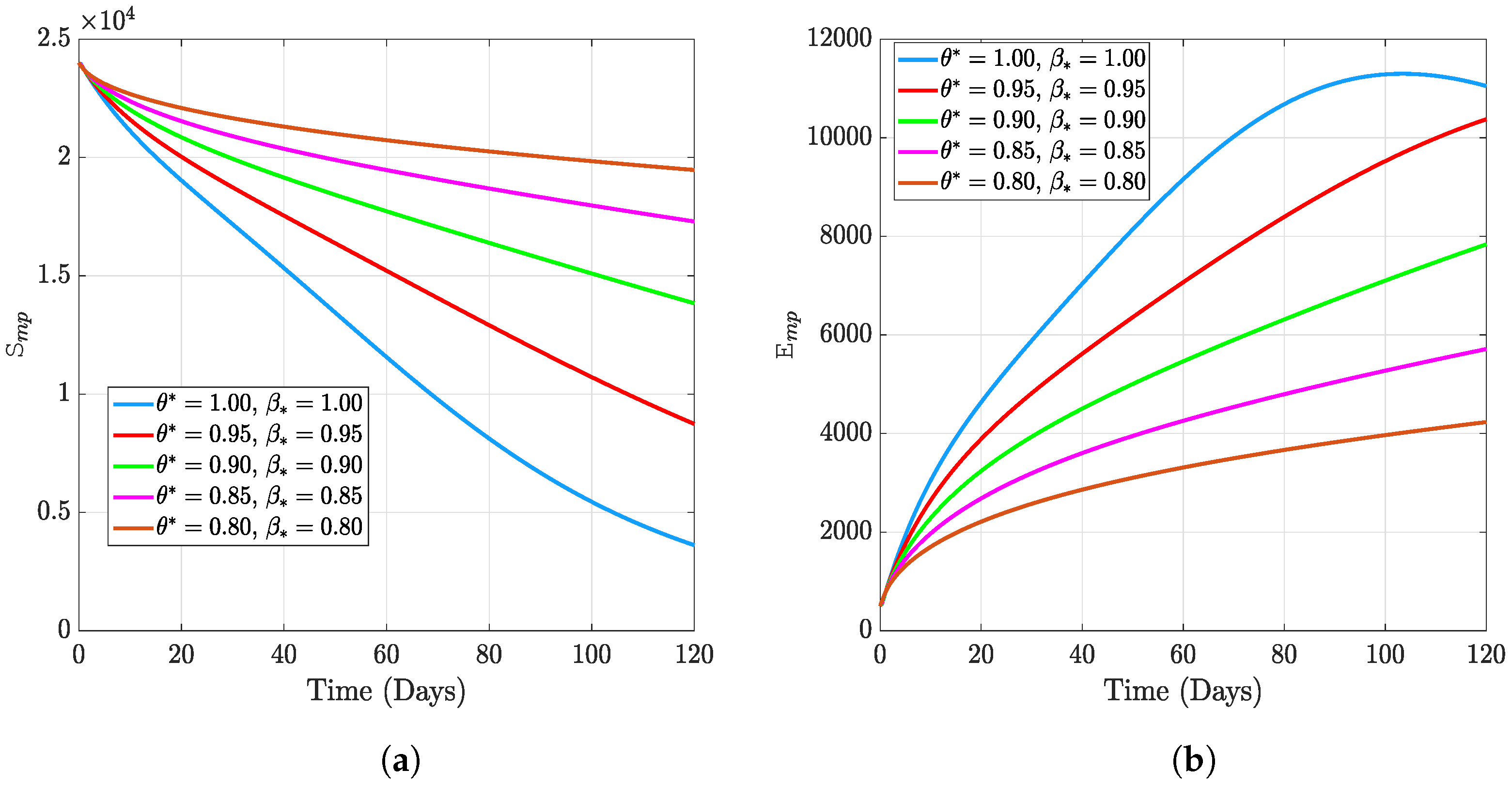
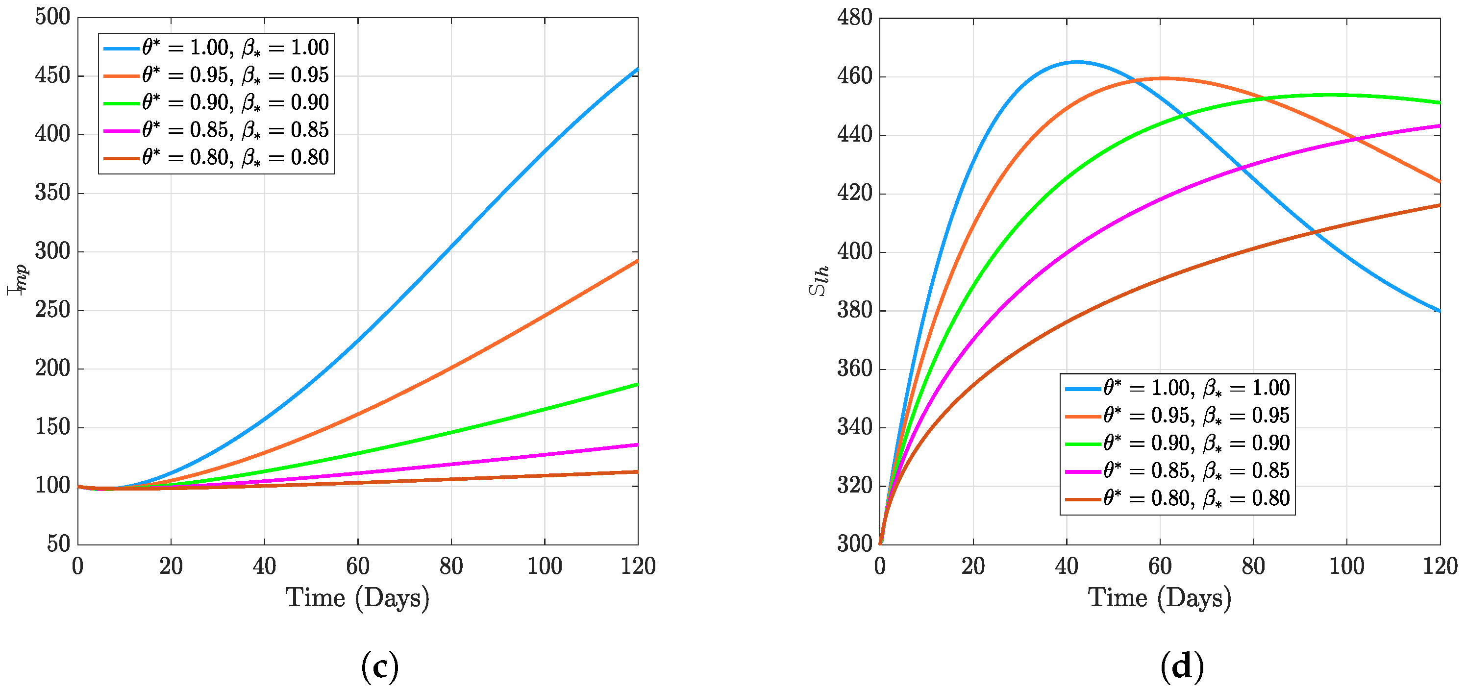
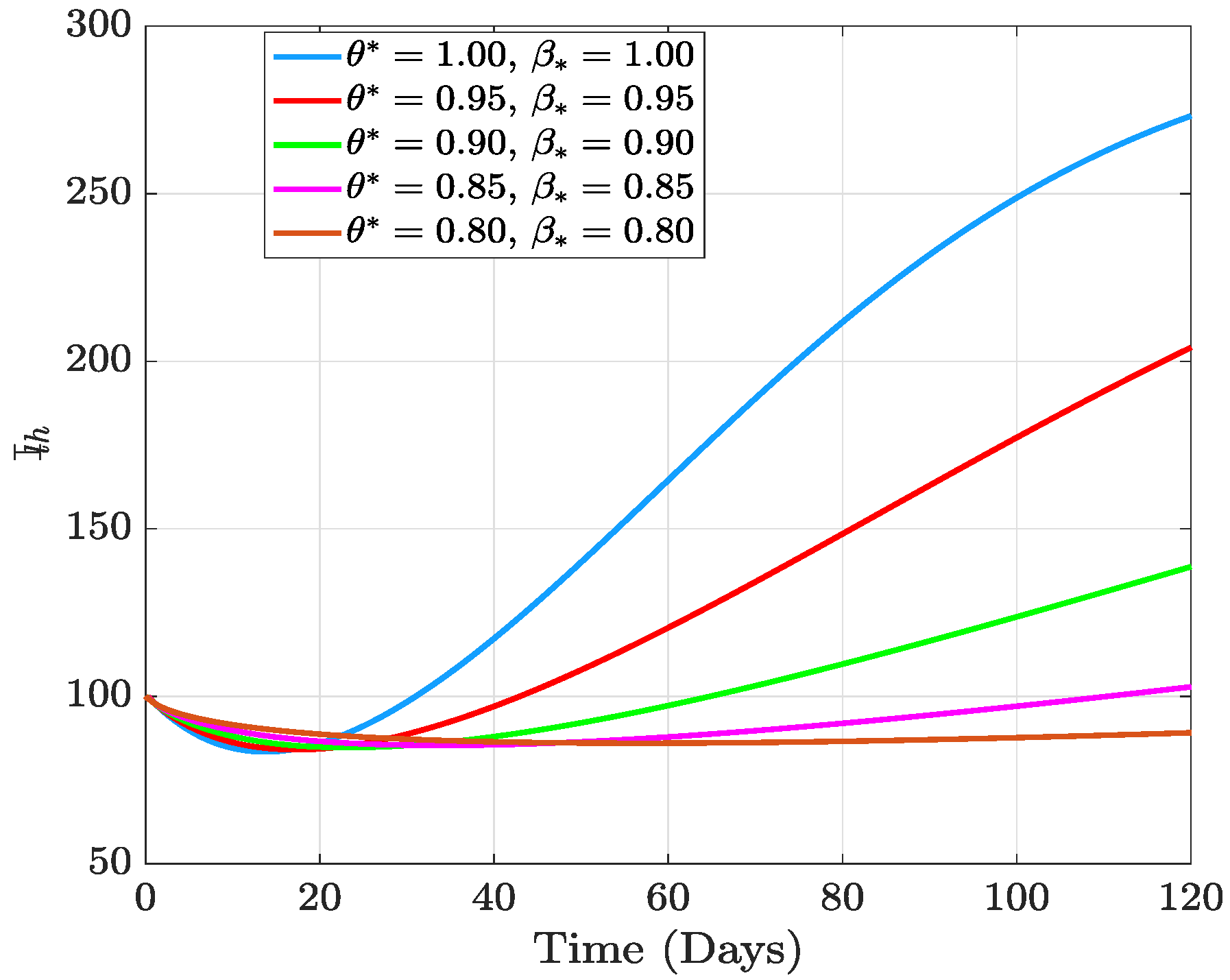
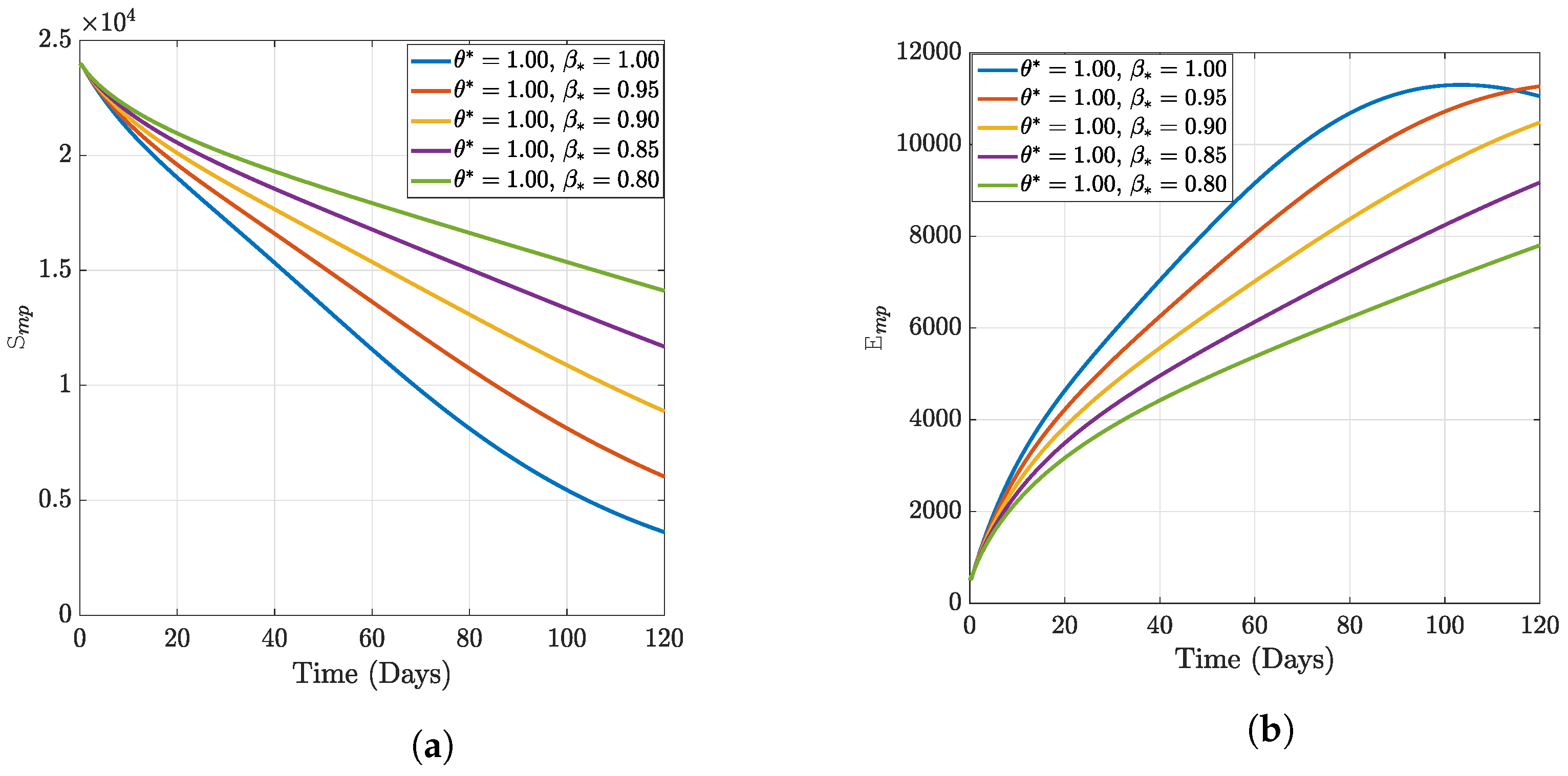
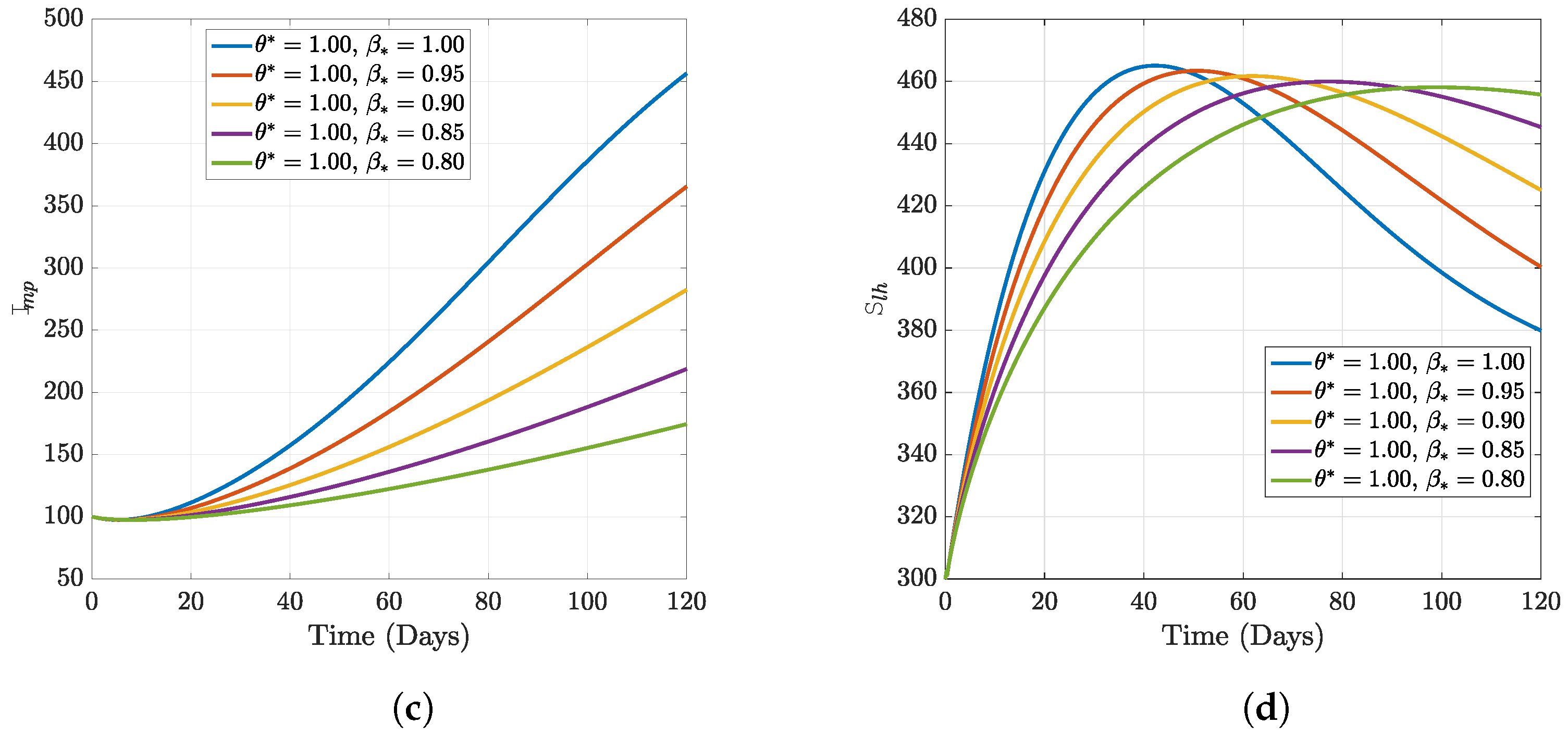
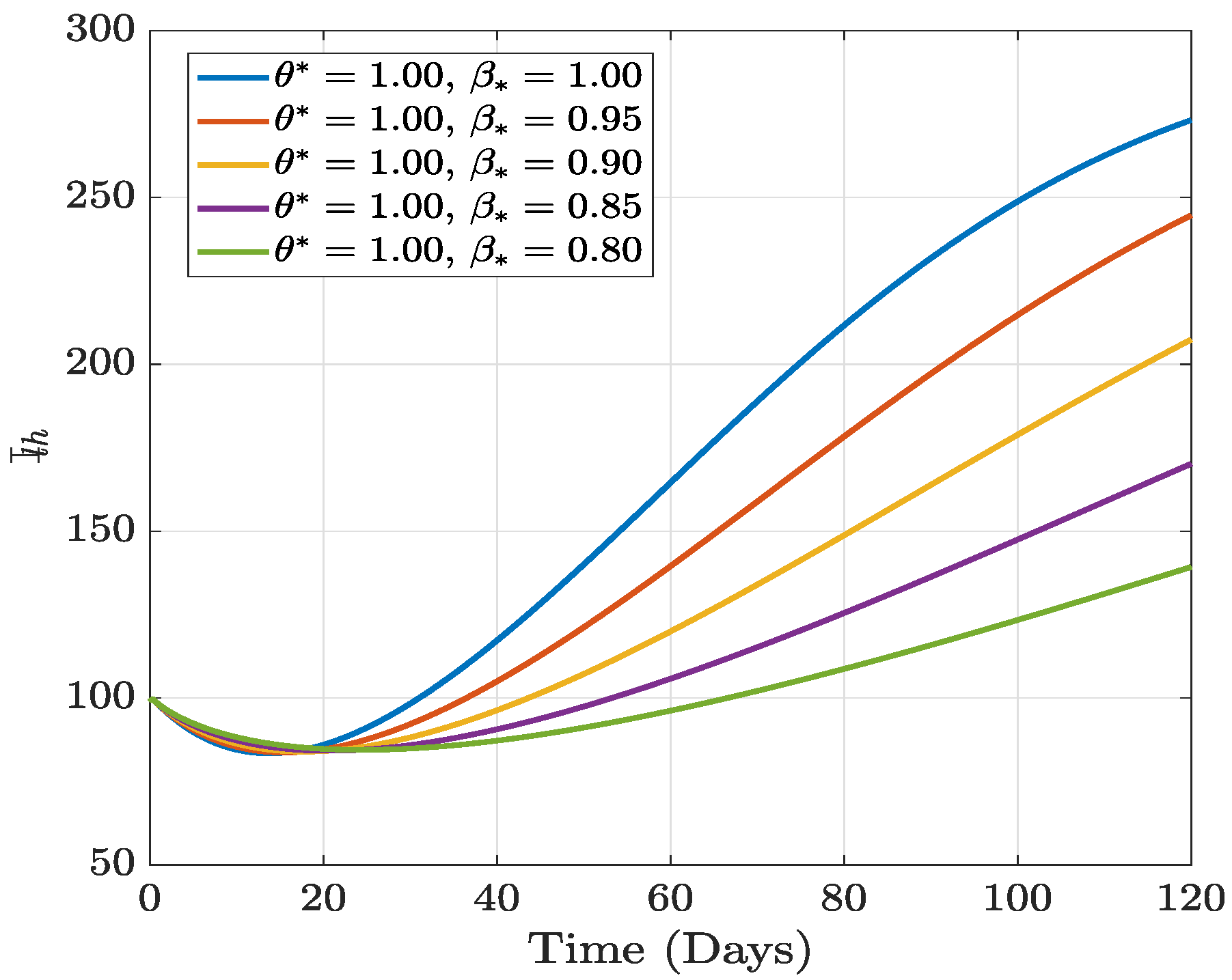
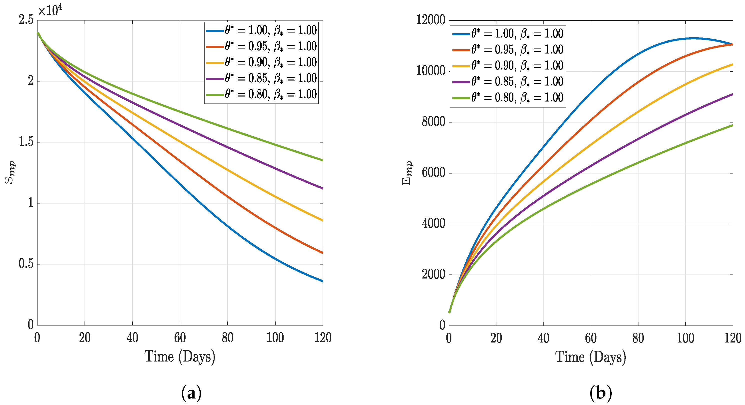
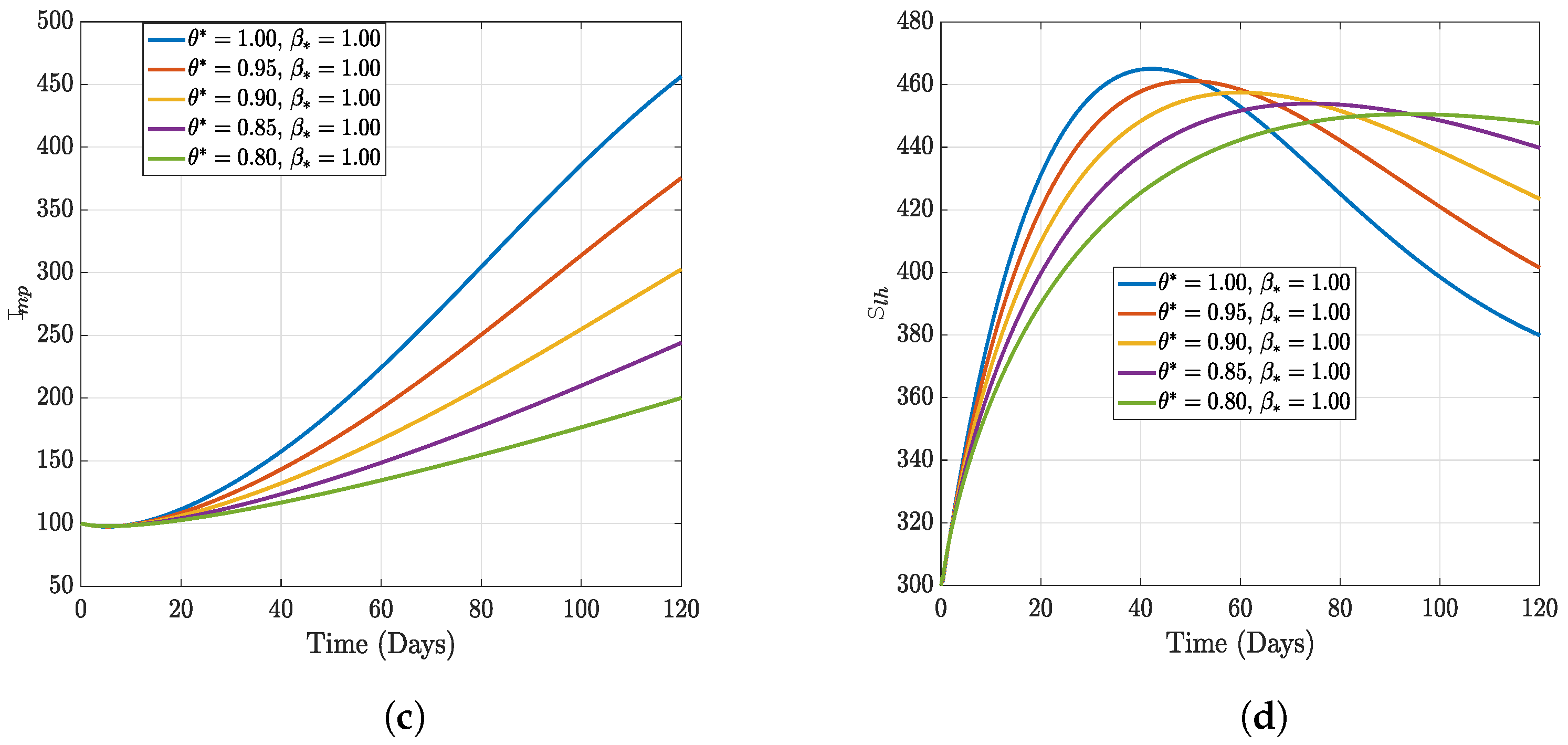
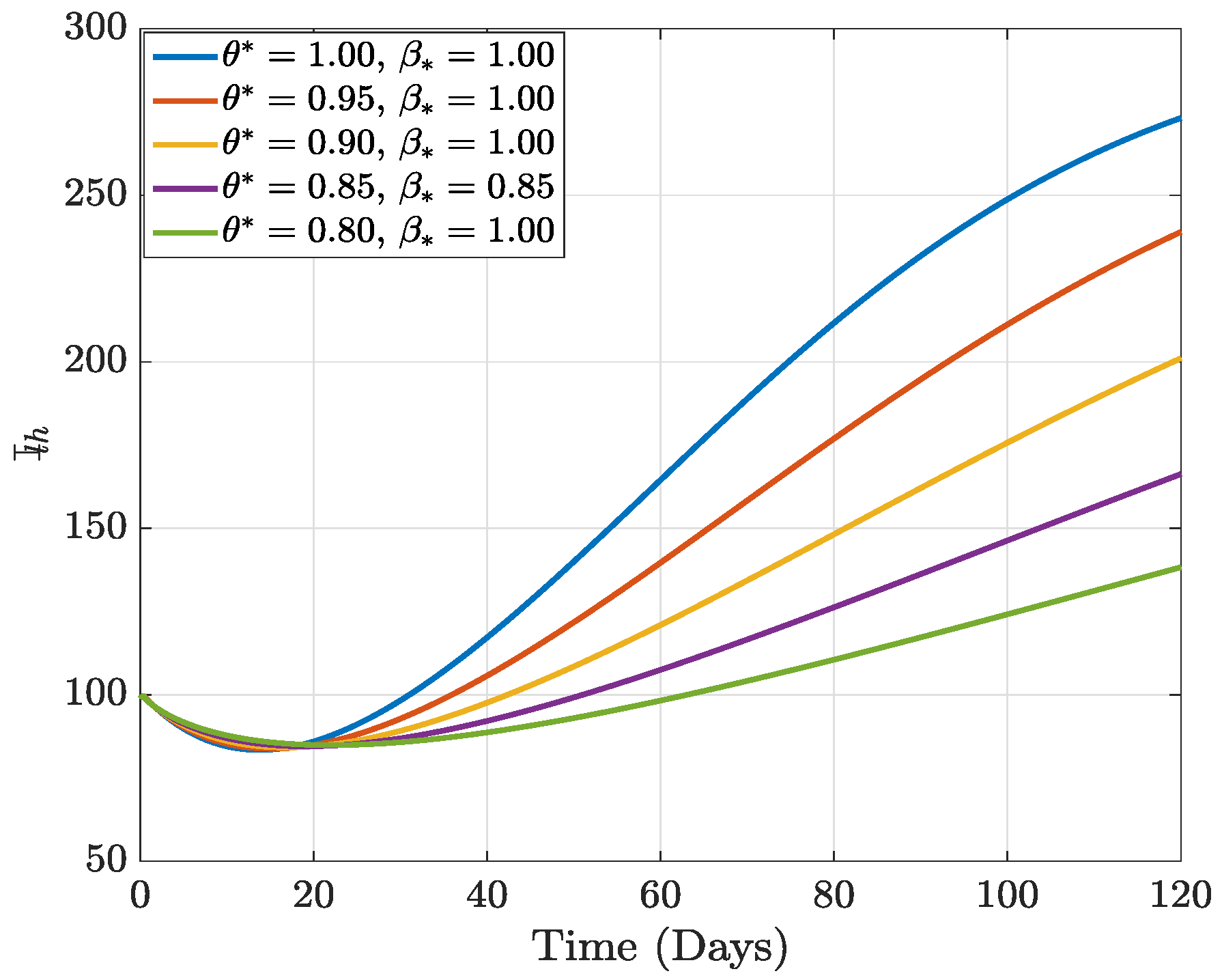
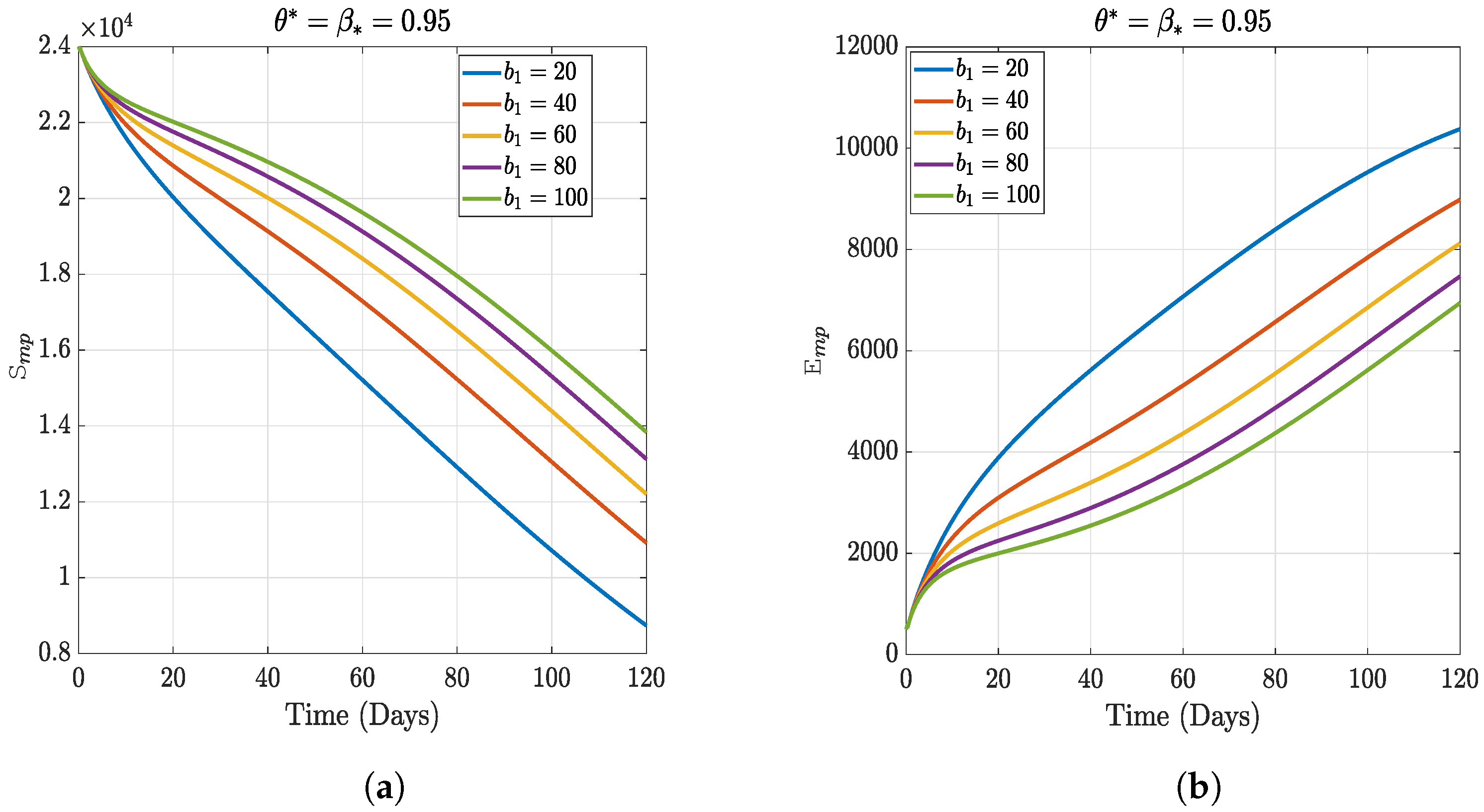
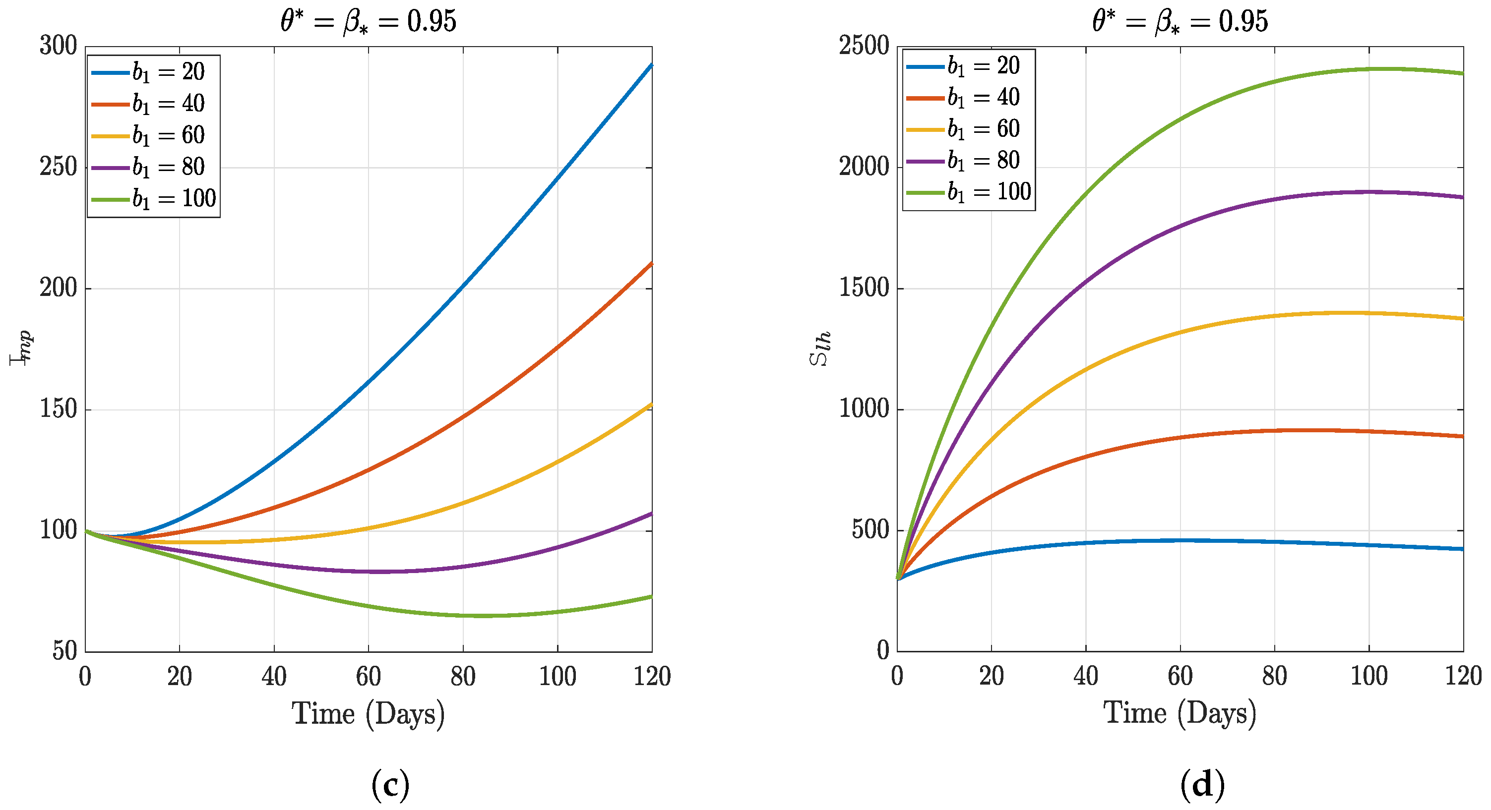
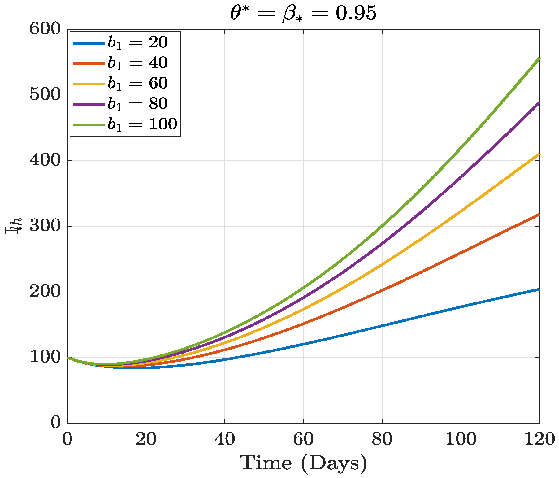
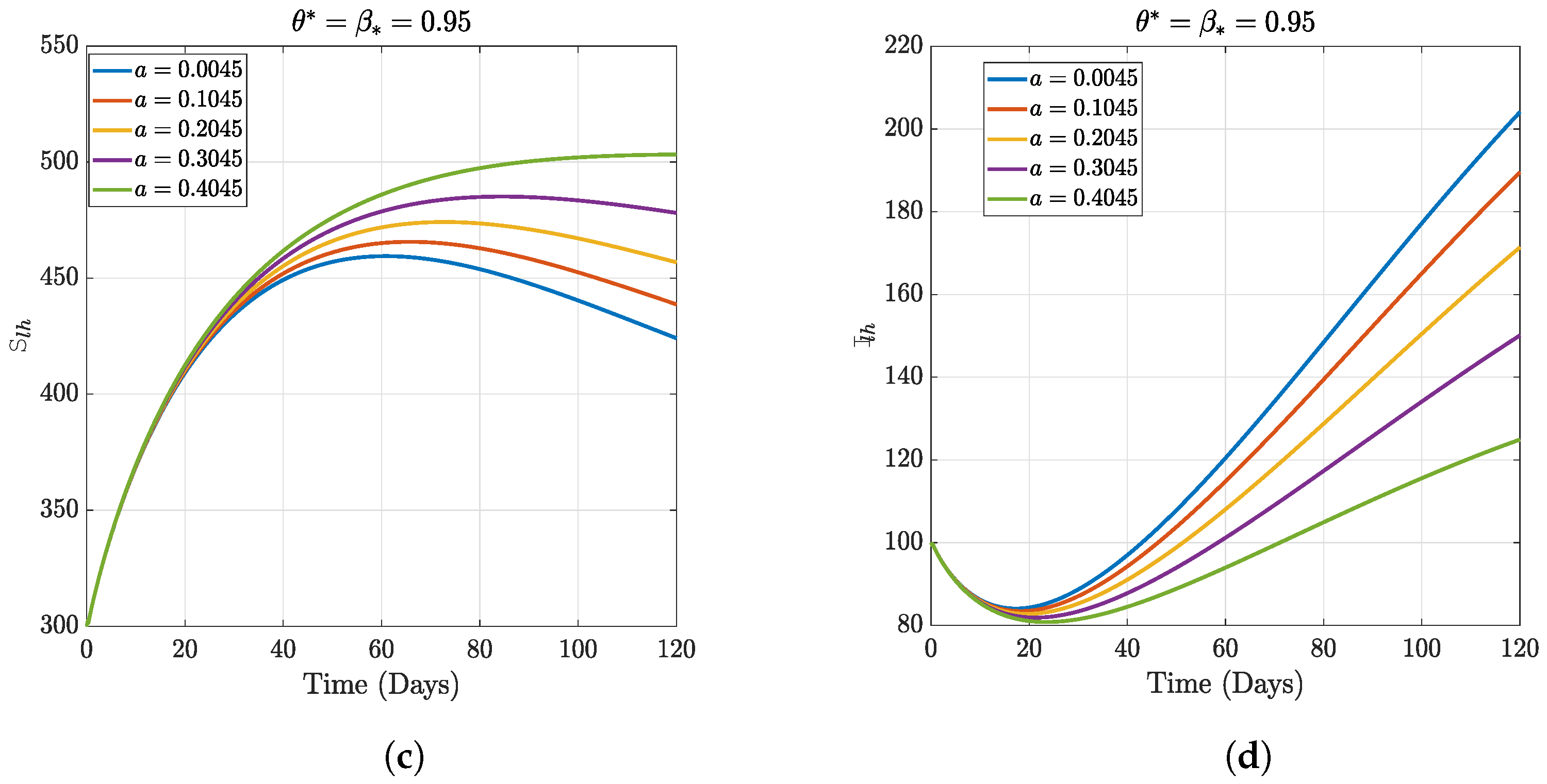
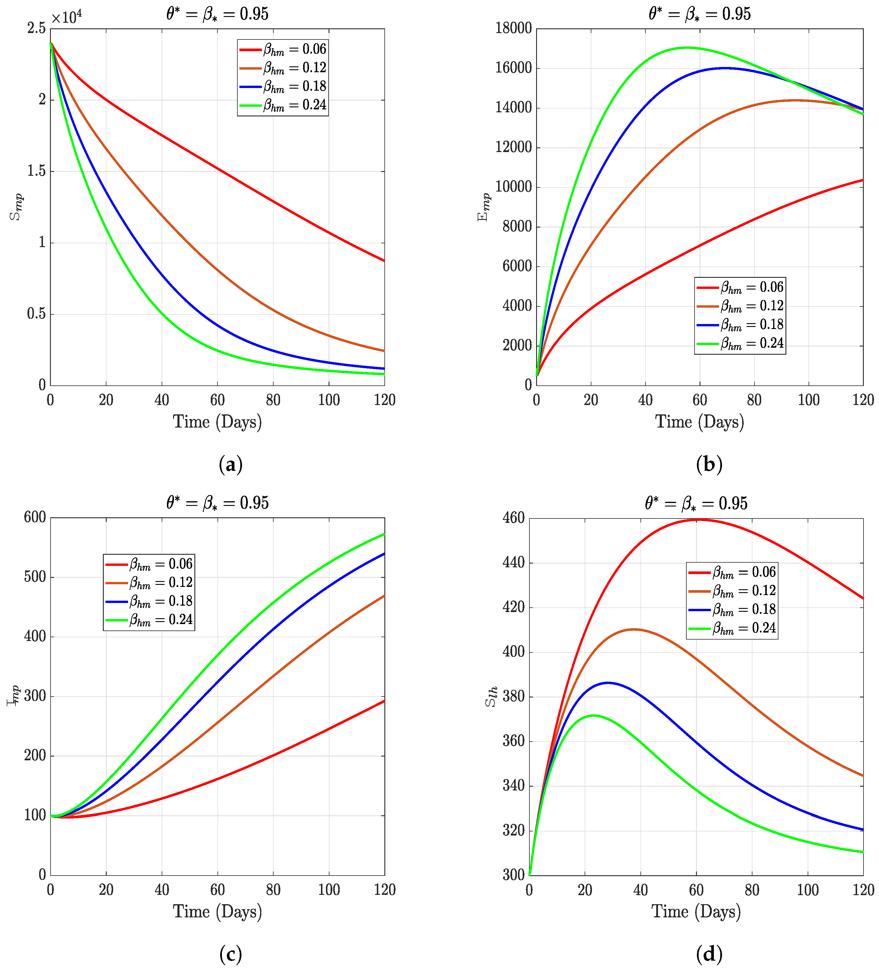
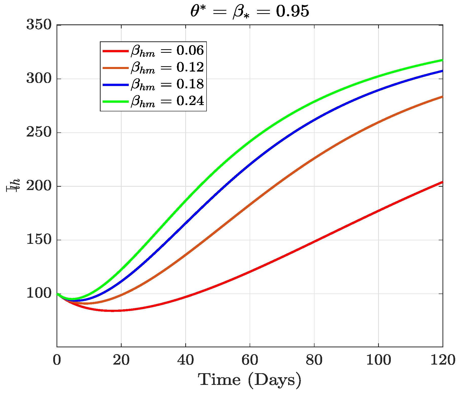
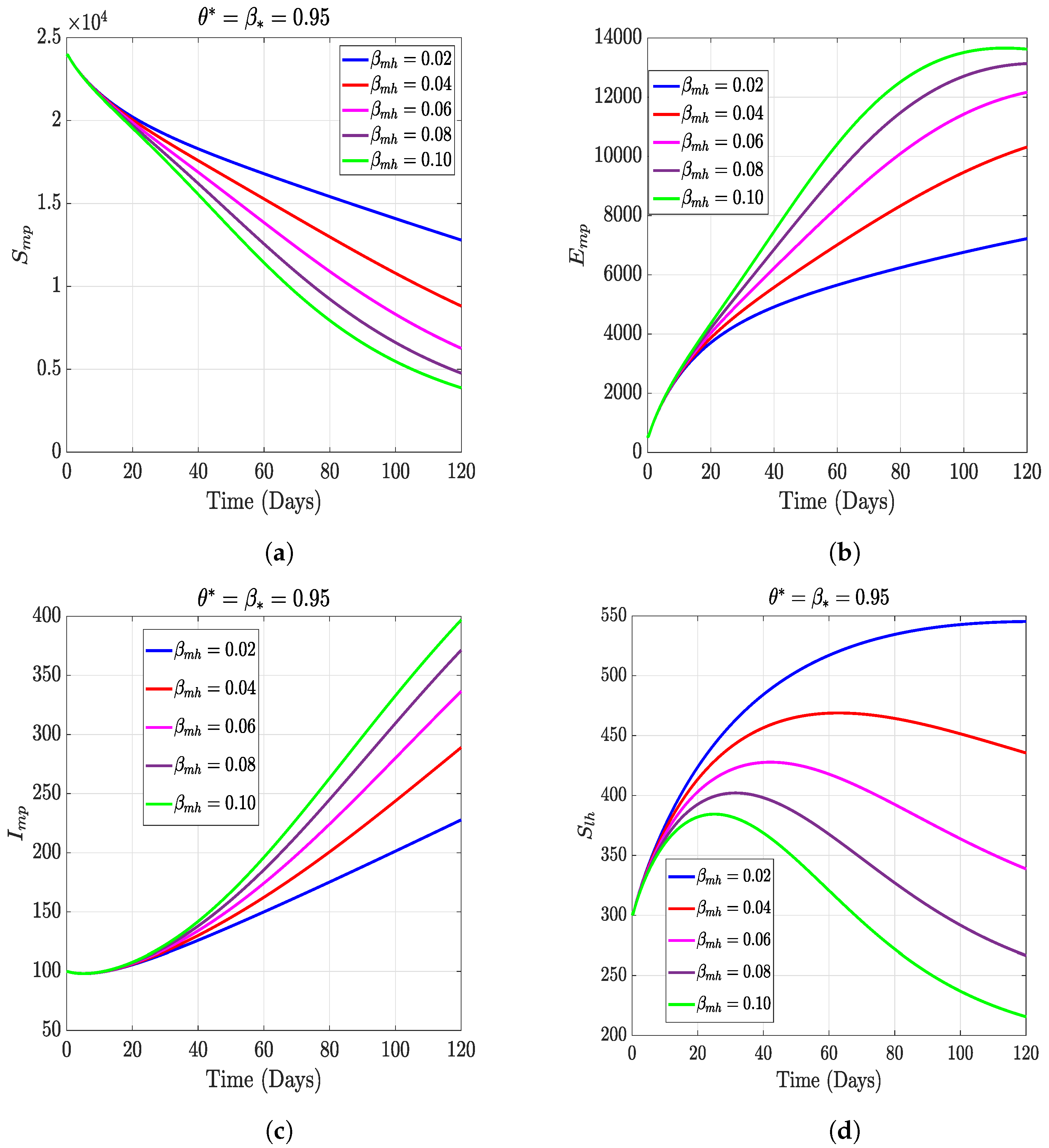
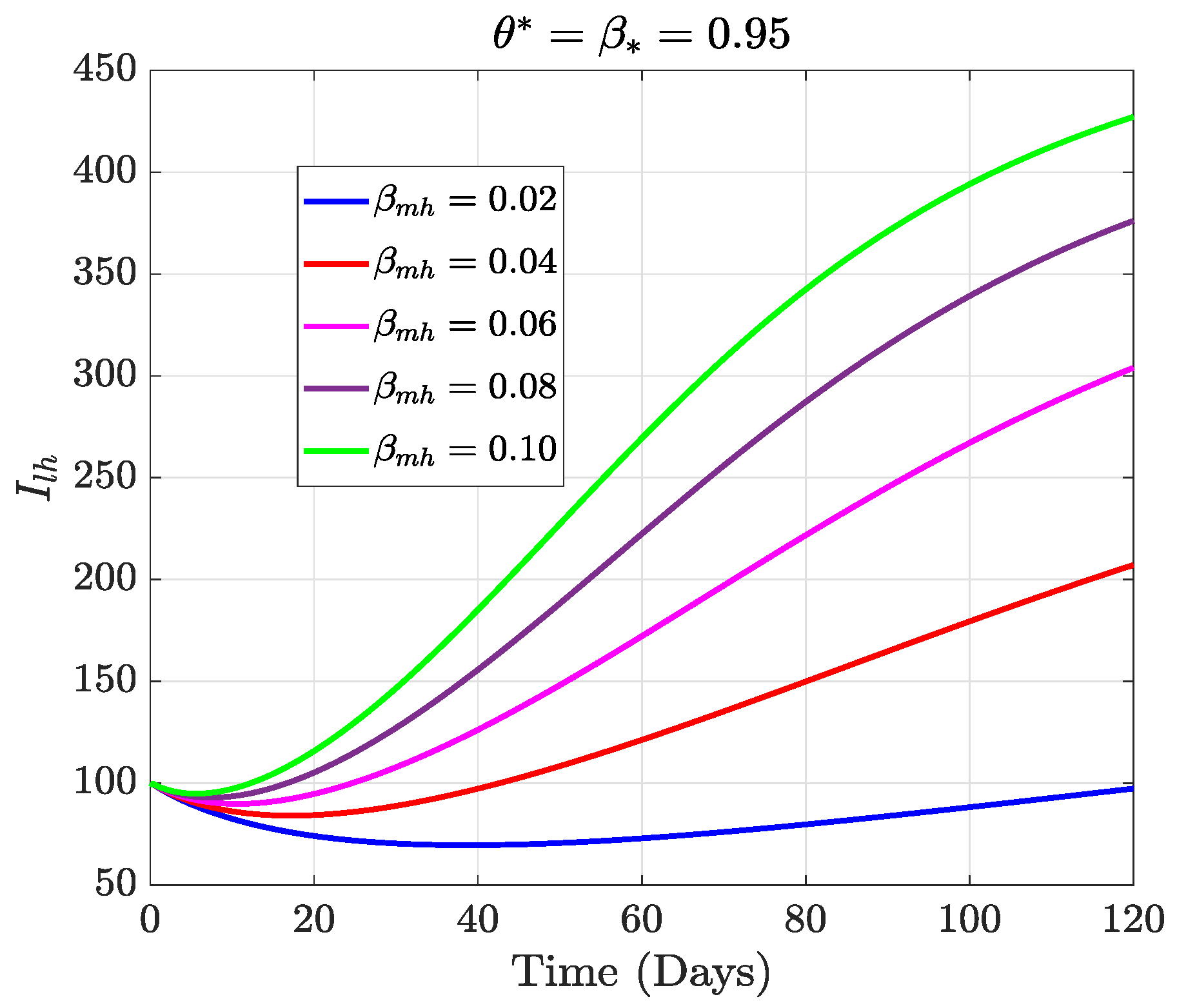
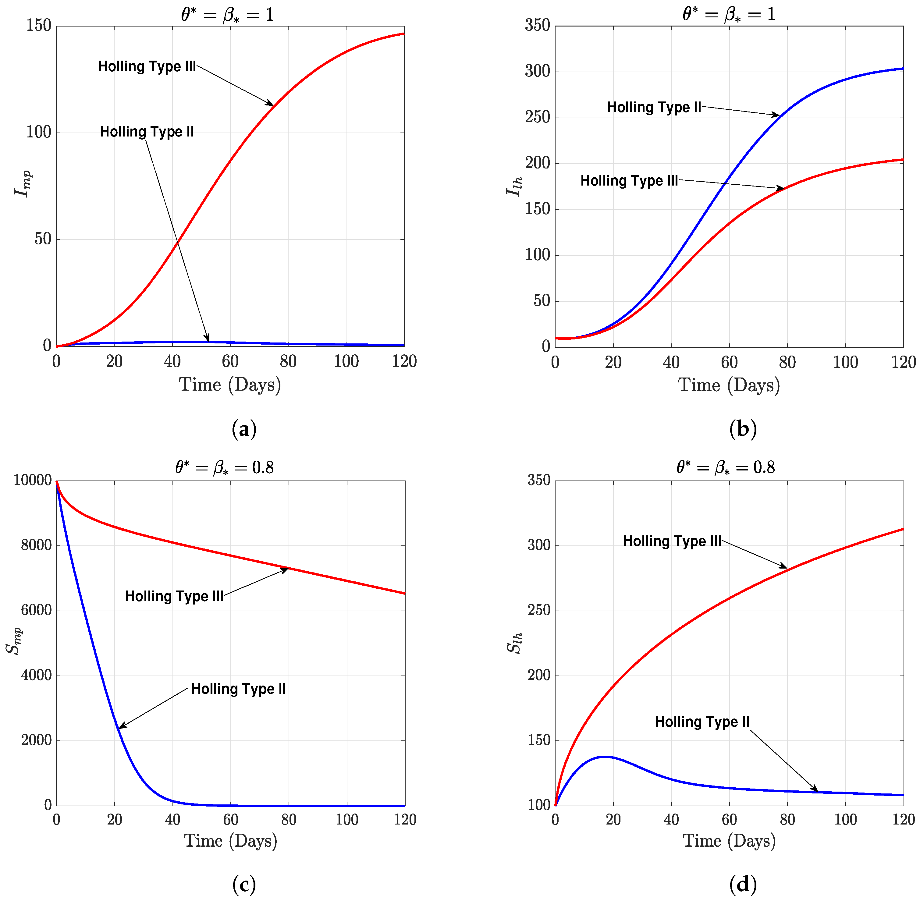
In this section, we present the results of the numerical simulation of the proposed model with Holling’s Type III using the parameters presented in Table 1 and the initial conditions We also compare the dynamics of Holling’s Type II and Holling’s Type III using the number of healthy maize, healthy leafhoppers, infected maize, and infected leafhoppers. In Figure 1 and Figure 2, we present the numerical simulation of our Caputo fractal-fractional model (4) with an integer order and also for different fractal-fractional orders. We observe from Figure 1a–d and Figure 2 that the integer-order model (when ) predicts lower healthy plants and higher unhealthy maize plants than the fractional-fractal order models. Thus, the integer order exaggerates the impact of MSVD on the maize field. In Figure 3 and Figure 4, we plot the simulation results by fixing the fractal dimension and varying the fractional order. We observe that for non-fractal models, higher fractional orders predict lower healthy maize plants and higher unhealthy plants (see Figure 3a–d and Figure 4, respectively). Moreover, for a fixed fractional order (see Figure 5a–d and Figure 6), increasing the fractal dimension, similar dynamics are observed as in fixing the fractal dimension and varying the fractional order. These results further strengthen the need to employ fractional-fractal models in studying infectious diseases. However, to derive the most benefit from these models, methods for fitting such models to observed data need to develop and improve. To study the effect of some epidemiological factors on the dynamics of MSVD in the maize plants, we solved the fractional-fractal model for varying values of those factors (parameters). In Figure 7a–d and Figure 8, the impact of the maize field’s invasion rate by the leafhoppers is presented by varying the invasion parameter . We observe that higher invasion rates have a devastating effect on the maize plants, leading to reduced healthy plants and increased unhealthy plants. This shows that if farms are projected to reduce the visitation of leafhoppers on farms, there will be an increase in healthy maize and a better subsequent yield. Further, to study the impact of the benefit derived from the consumption of maize plants by the leafhopper population, we simulated the model for varying values of the conversion rate parameter a (Figure 9a–d). It is observed that higher conversion rates lead to lower exposed maize plants. This is attributed to the fact that as more and more of the plants are visited and consumed, fewer remain unvisited/susceptible to exposure to MSVD. Figure 10a–d and Figure 11 show the dynamics of varying the maize streak virus transmission rate from infected leafhoppers to maize when the fractal and fractional orders are kept at 0.95. Thus, we noticed that an increase in the maize streak virus transmission rate from infected leafhoppers to maize leads to a reduction in healthy maize and healthy leafhoppers but an increase in infected compartments. Figure 12a–d and Figure 13 show the dynamics of varying the maize streak virus transmission rate from infected plants to leafhoppers when the fractal and fractional orders are kept at 0.95. We noticed that an increase in the maize streak virus transmission rate from infected maize to leafhopper similarly leads to a reduction in healthy maize and healthy leafhoppers but an increase in infected compartments. Therefore, this indicates that when preventive measures are taken to reduce and , it will reduce the low-yielding effect of maize due to the maize streak virus disease on farms. Finally, in Figure 14a–d we present the numerical simulation of the model for the effect of the Holling’s Type II and Holling’s Type III responses. We observed that Holling’s Type III predicts a higher population of healthy and unhealthy maize plants than Type II.

Table 1.
Parameter Description and Values for the Caputo Fractal-Fractional Model.
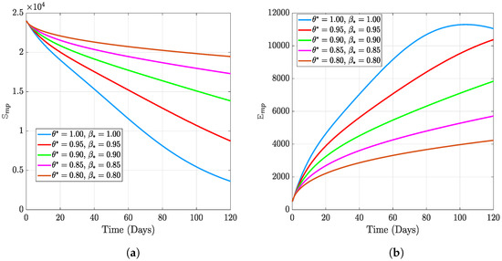
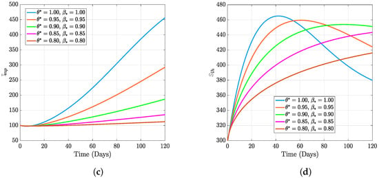
Figure 1.
Numerical results of varying both fractal order and fractional order with fixed fractal dimension.
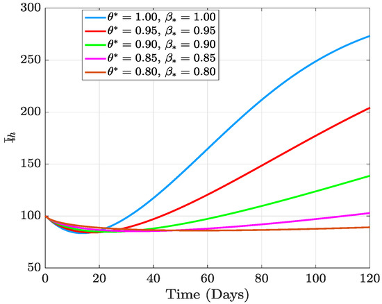
Figure 2.
Numerical results of varying both fractal order and fractional order with fixed fractal dimension on infected leafhoppers.
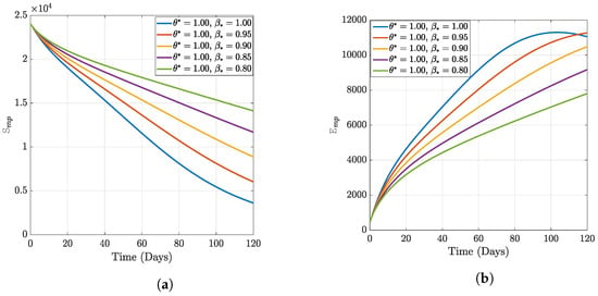
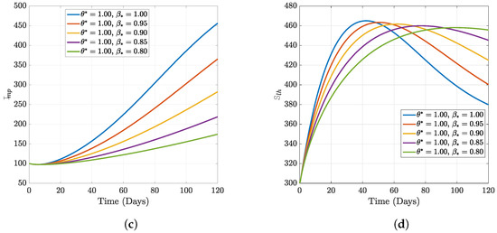
Figure 3.
Numerical results of varying fractional order with fixed fractal dimension.
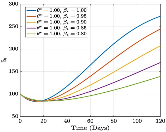
Figure 4.
Numerical results of varying fractional order with fixed fractal dimension on infected leafhoppers.
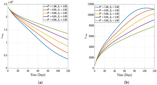
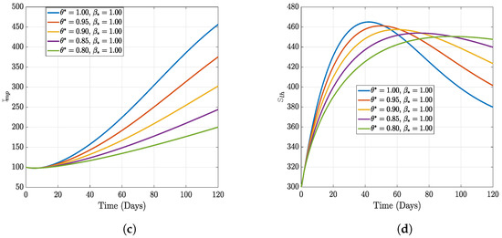
Figure 5.
Numerical results of varying fractal order with fixed fractional order.
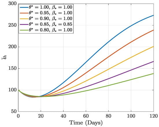
Figure 6.
Numerical results of varying fractal order with fixed fractional order on infected leafhoppers.
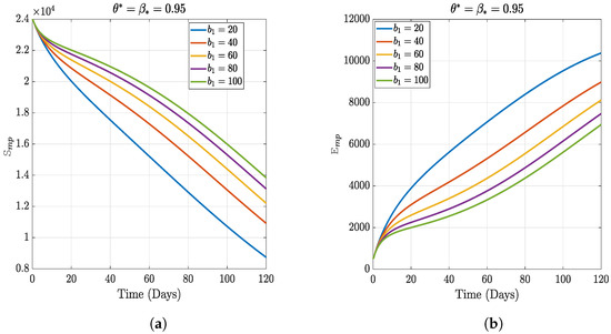
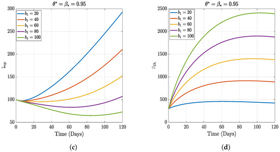
Figure 7.
Numerical results of varying the relative increase rate of leafhoppers.
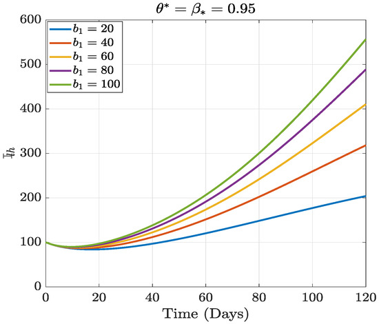
Figure 8.
Numerical results of varying the relative increase rate of leafhoppers.
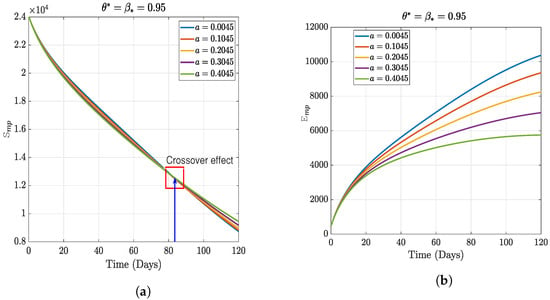

Figure 9.
Numerical results of varying the rate of conversion.
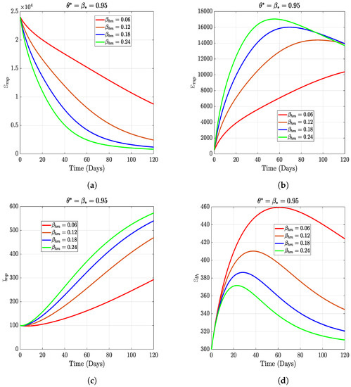
Figure 10.
The dynamical effect of varying the maize streak virus transmission rate from infected leafhoppers to maize on each model compartment.
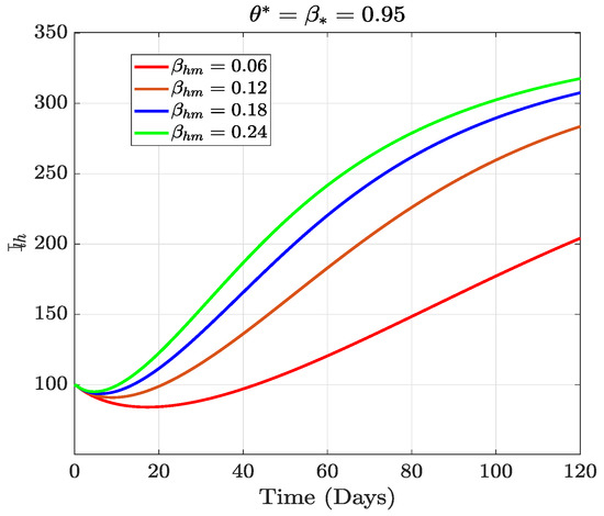
Figure 11.
The dynamical effect of varying the rate of maize streak virus transmission from infected leafhoppers to maize.
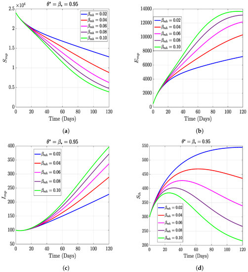
Figure 12.
The dynamical effect of varying the rate of maize streak virus transmission from infected plants to leafhoppers.
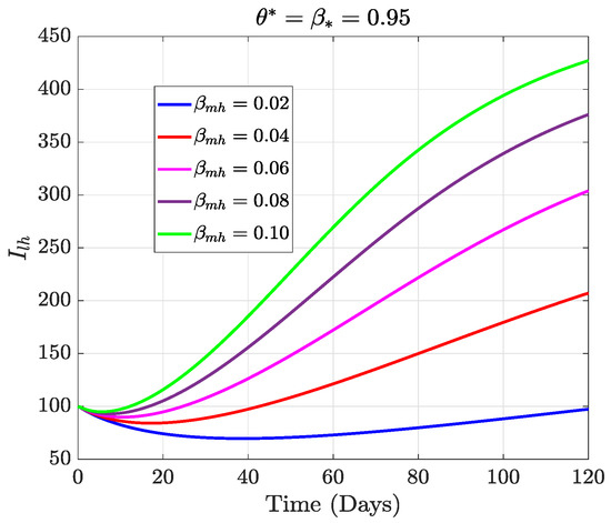
Figure 13.
The dynamical effect of varying the rate of maize streak virus transmission from infected plants to leafhoppers on infected leafhoppers.
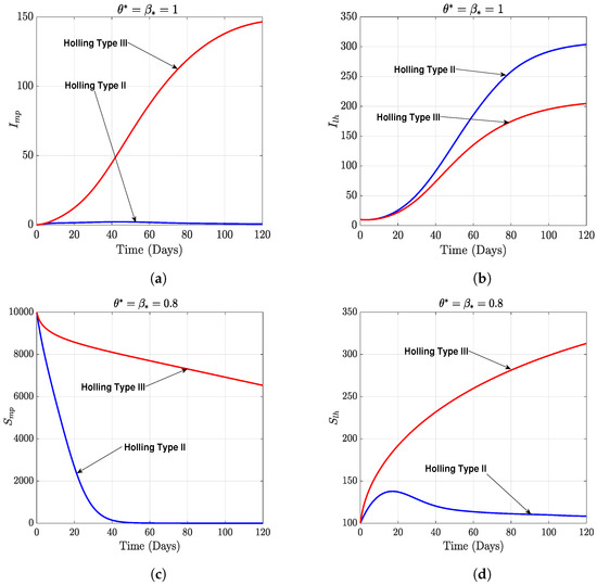
Figure 14.
The dynamical effect of Holling’s Type II and Holling’s Type III functional responses.
6. Conclusions
Epidemiological models are essential because they provide helpful biological explanations and possible ways to prevent and control infectious diseases. We used Holling’s Type III and fractal-fractional derivatives to improve the model in [7] to examine the dynamics of maize streak virus disease. The Banach principle, which shows that all continuous functions under a specific norm belong to the same subclass, was used to study whether or not there are solutions. The Lipschitz property illustrated that the Caputo fractal-fractional model of maize streak disease had a unique solution. The stability test for solutions of the given Caputo fractal-fractional model was studied using Ulam–Hyers and Ulam–Hyers–Rassias and their extended forms. The numerical strategy for the fractal-fractional maize streak model was provided by utilizing the Adams–Bashforth approach. Finally, several simulation results highlight the effect of the fractal-fractional orders and model parameters on disease dynamics. The increased leafhopper visitation of maize fields is shown to have devastating effects on healthy plants and hence efforts should be made to protect maize fields. These efforts could include the use of pesticides and MSVD-resistant strains of maize. Moreover, natural predators of leafhoppers could be introduced into the maize fields to help control the population of leafhoppers when they visit. The effect of natural predators of leafhoppers on the dynamics of MSVD is the subject of our next research on MSVD. Future research directions should aim at developing a resistant maize varieties mathematical model, using integrated pest management strategies, increase awareness and education about the disease among farmers, and develop a fractal-fractional reaction–diffusion model of maize streak virus disease.
Author Contributions
Conceptualization, J.A.-P., B.S., E.O. and J.K.K.A.; methodology, J.A.-P., B.S., E.O. and J.K.K.A.; software, J.A.-P., B.S., E.O. and J.K.K.A.; validation, J.A.-P., B.S., E.O. and J.K.K.A.; formal analysis, J.A.-P., B.S., E.O. and J.K.K.A.; investigation, J.A.-P., B.S., E.O. and J.K.K.A.; resources, J.A.-P., B.S., E.O. and J.K.K.A.; data curation, J.A.-P., B.S., E.O. and J.K.K.A.; writing—original draft preparation, J.A.-P., B.S., E.O. and J.K.K.A.; writing—review and editing, J.A.-P., B.S., E.O. and J.K.K.A.; visualization, J.A.-P., B.S., E.O. and J.K.K.A.; supervision, J.A.-P., B.S., E.O. and J.K.K.A.; project administration, J.A.-P., B.S., E.O. and J.K.K.A. All authors have read and agreed to the published version of the manuscript.
Funding
This research received no external funding.
Data Availability Statement
No data were used for this study.
Conflicts of Interest
The authors declare no conflict of interest.
Abbreviations
The following abbreviations are used in this manuscript:
| MDPI | Multidisciplinary Digital Publishing Institute |
| DOAJ | Directory of open access journals |
| TLA | Three-letter acronym |
| LD | Linear dichroism |
References
- FAO. International Year of Plant Health—Final Report; FAO: Rome, Italy, 2021. [Google Scholar]
- Collins, O.C.; Duffy, K.J. Optimal control of maize foliar diseases using the plants population dynamics. Acta Agric. Scand. Sect. B Soil Plant Sci. 2016, 66, 20–26. [Google Scholar] [CrossRef]
- Aloyce, W.; Kuznetsov, D.; Luboobi, L. A mathematical model for the mlnd dynamics and sensitivity analysis in a maize population. Asian J. Math. Appl. 2017, 2017, ama0435. [Google Scholar]
- Alemneh, H.T.; Makinde, O.D.; Theuri, D.M. Ecoepidemiological Model and Analysis of MSV Disease Transmission Dynamics in Maize Plant. Int. J. Math. Math. Sci. 2019, 2019, 7965232. [Google Scholar] [CrossRef]
- Alemneh, H.T.; Makinde, O.D.; Theuri, D.M. Optimal Control Model and Cost Effectiveness Analysis of Maize Streak Virus Pathogen Interaction with Pest Invasion in Maize Plant. Egypt. J. Basic Appl. Sci. 2020, 7, 180–193. [Google Scholar] [CrossRef]
- Alemneh, H.T.; Kassa, A.S.; Godana, A.A. An optimal control model with cost effectiveness analysis of Maize streak virus disease in maize plant. Infect. Dis. Model. 2021, 6, 169–182. [Google Scholar]
- Seidu, B.; Asamoah, J.K.K.; Wiah, E.N.; Ackora-Prah, J. A comprehensive cost-effectiveness analysis of control of maize streak virus disease with Holling’s Type II predation form and standard incidence. Results Phys. 2022, 40, 105862. [Google Scholar]
- Ayembillah, A.F.O.; Seidu, B.; Bornaa, C. Mathematical modeling of the dynamics of maize streak virus disease (MSVD). Math. Model. Control 2022, 2, 153–164. [Google Scholar]
- Asamoah, J.K.K. Fractal–fractional model and numerical scheme based on Newton polynomial for Q fever disease under Atangana–Baleanu derivative. Results Phys. 2022, 34, 105189. [Google Scholar]
- Atangana, A. Fractal-fractional differentiation and integration: Connecting fractal calculus and fractional calculus to predict complex system. Chaos Solitons Fractals 2017, 102, 396–406. [Google Scholar]
- Owolabi, K.M.; Atangana, A.; Akgul, A. Modelling and analysis of fractal-fractional partial differential equations: Application to reaction-diffusion model. Alex. Eng. J. 2020, 59, 2477–2490. [Google Scholar]
- Atangana, A.; Qureshi, S. Modeling attractors of chaotic dynamical systems with fractal–fractional operators. Chaos Solitons Fractals 2019, 123, 320–337. [Google Scholar] [CrossRef]
- Atangana, A.; Araz, S.İ. New numerical approximation for Chua attractor with fractional and fractal-fractional operators. Alex. Eng. J. 2020, 59, 3275–3296. [Google Scholar]
- Atangana, A. Modelling the spread of COVID-19 with new fractal-fractional operators: Can the lockdown save mankind before vaccination? Chaos Solitons Fractals 2020, 136, 109860. [Google Scholar] [PubMed]
- Ali, Z.; Rabiei, F.; Shah, K.; Khodadadi, T. Modeling and analysis of novel COVID-19 under fractal-fractional derivative with case study of Malaysia. Fractals 2021, 29, 2150020. [Google Scholar]
- Saad, K.M.; Alqhtani, M.; Gómez-Aguilar, J. Fractal-fractional study of the hepatitis C virus infection model. Results Phys. 2020, 19, 103555. [Google Scholar]
- Shah, K.; Arfan, M.; Mahariq, I.; Ahmadian, A.; Salahshour, S.; Ferrara, M. Fractal-fractional mathematical model addressing the situation of corona virus in Pakistan. Results Phys. 2020, 19, 103560. [Google Scholar] [PubMed]
- Abdulwasaa, M.A.; Abdo, M.S.; Shah, K.; Nofal, T.A.; Panchal, S.K.; Kawale, S.V.; Abdel-Aty, A.H. Fractal-fractional mathematical modeling and forecasting of new cases and deaths of COVID-19 epidemic outbreaks in India. Results Phys. 2021, 20, 103702. [Google Scholar] [PubMed]
- Ahmad, S.; Ullah, A.; Abdeljawad, T.; Akgül, A.; Mlaiki, N. Analysis of fractal-fractional model of tumor-immune interaction. Results Phys. 2021, 25, 104178. [Google Scholar] [CrossRef]
- Al Qurashi, M.M. Role of fractal-fractional operators in modeling of rubella epidemic with optimized orders. Open Phys. 2020, 18, 1111–1120. [Google Scholar] [CrossRef]
- Fatmawati; Khan, M.A.; Alfiniyah, C.; Alzahrani, E. Analysis of dengue model with fractal-fractional Caputo–Fabrizio operator. Adv. Differ. Equations 2020, 2020, 1–23. [Google Scholar]
- Akgül, A.; Ahmed, N.; Raza, A.; Iqbal, Z.; Rafiq, M.; Rehman, M.; Baleanu, D. A fractal fractional model for cervical cancer due to human papillomavirus infection. Fractals 2021, 29, 2140015-19. [Google Scholar] [CrossRef]
- Gomez-Aguilar, J.; Cordova-Fraga, T.; Abdeljawad, T.; Khan, A.; Khan, H. Analysis of fractal–fractional malaria transmission model. Fractals 2020, 28, 2040041. [Google Scholar] [CrossRef]
- Sinan, M.; Ahmad, H.; Ahmad, Z.; Baili, J.; Murtaza, S.; Aiyashi, M.; Botmart, T. Fractional mathematical modeling of malaria disease with treatment & insecticides. Results Phys. 2022, 34, 105220. [Google Scholar]
- Ahmad, Z.; Bonanomi, G.; di Serafino, D.; Giannino, F. Transmission dynamics and sensitivity analysis of pine wilt disease with asymptomatic carriers via fractal-fractional differential operator of Mittag-Leffler kernel. Appl. Numer. Math. 2023, 185, 446–465. [Google Scholar] [CrossRef]
- Malik, A.; Alkholief, M.; Aldakheel, F.M.; Khan, A.A.; Ahmad, Z.; Kamal, W.; Gatasheh, M.K.; Alshamsan, A. Sensitivity analysis of COVID-19 with quarantine and vaccination: A fractal-fractional model. Alex. Eng. J. 2022, 61, 8859–8874. [Google Scholar] [CrossRef]
- Rezapour, S.; Asamoah, J.K.K.; Hussain, A.; Ahmad, H.; Banerjee, R.; Etemad, S.; Botmart, T. A theoretical and numerical analysis of a fractal-fractional two-strain model of meningitis. Results Phys. 2022, 39, 105775. [Google Scholar] [CrossRef]
- Samet, B.; Vetro, C.; Vetro, P. Fixed point theorems for α–ψ-contractive type mappings. Nonlinear Anal. Theory Methods Appl. 2012, 75, 2154–2165. [Google Scholar] [CrossRef]
- Asamoah, J.K.K.; Bornaa, C.; Seidu, B.; Jin, Z. Mathematical analysis of the effects of controls on transmission dynamics of SARS-CoV-2. Alex. Eng. J. 2020, 59, 5069–5078. [Google Scholar] [CrossRef]
- Yang, X.; Chen, L.; Chen, J. Permanence and positive periodic solution for the single-species nonautonomous delay diffusive models. Comput. Math. Appl. 1996, 32, 109–116. [Google Scholar] [CrossRef]
- Granas, A.; Dugundji, J. Fixed Point Theory; Springer: Berlin/Heidelberg, Germany, 2003; Volume 14. [Google Scholar]
- Hyers, D.H. On the stability of the linear functional equation. Proc. Natl. Acad. Sci. USA 1941, 27, 222–224. [Google Scholar] [CrossRef]
- Rassias, T.M. On the stability of the linear mapping in Banach spaces. Proc. Am. Math. Soc. 1978, 72, 297–300. [Google Scholar] [CrossRef]
- Bosque-Pérez, N.A. Eight decades of maize streak virus research. Virus Res. 2000, 71, 107–121. [Google Scholar] [CrossRef] [PubMed]
- GreenLife. MAIZE: Harvesting Period: In General, Maize Requires 120 Days (12 Weeks) to Reach Maturity. However, Early Maturing Varieties Take 75–80 Days. Available online: http://gis4agricgh.net/POLICIES/commodities/Commodity%20Profile_maize.pdf (accessed on 15 December 2022).
- BioNet-Eatrinet. Cicadulina mbila (Naude)-Maize Leafhopper. Available online: https://keys.lucidcentral.org/keys/v3/eafrinet/maize_pests/key/maize_pests/Media/Html/Cicadulina_mbila_(Naude)_-_Maize_Leafhopper.htm (accessed on 15 December 2022).
- Alemneh, H.T.; Makinde, O.D.; Theuri, D.M. Mathematical modelling of msv pathogen interaction with pest invasion on maize plant. Glob. J. Pure Appl. Math. 2019, 15, 55–79. [Google Scholar]
Disclaimer/Publisher’s Note: The statements, opinions and data contained in all publications are solely those of the individual author(s) and contributor(s) and not of MDPI and/or the editor(s). MDPI and/or the editor(s) disclaim responsibility for any injury to people or property resulting from any ideas, methods, instructions or products referred to in the content. |
© 2023 by the authors. Licensee MDPI, Basel, Switzerland. This article is an open access article distributed under the terms and conditions of the Creative Commons Attribution (CC BY) license (https://creativecommons.org/licenses/by/4.0/).

