Abstract
Proper control is necessary for ensuring that UAVs successfully navigate their surroundings and accomplish their intended tasks. Undoubtedly, a perfect control technique can significantly improve the performance and reliability of UAVs in a wide range of applications. Motivated by this, in the current paper, a new data-driven-based fractional-order control technique is proposed to address this issue and enable UAVs to track desired trajectories despite the presence of external disturbances and uncertainties. The control approach combines a deep neural network with a robust fractional-order controller to estimate uncertainties and minimize the impact of unknown disturbances. The design procedure for the controller is outlined in the paper. To evaluate the proposed technique, numerical simulations are performed for two different desired paths. The results show that the control method performs well in the presence of dynamic uncertainties and control input constraints, making it a promising approach for enabling UAVs to track desired trajectories in challenging environments.
1. Introduction
Unmanned aerial vehicles (UAVs) have the potential to be used for a wide range of applications, including surveillance, transportation, and environmental monitoring, among others [1,2]. However, controlling the trajectory and behavior of UAVs can be challenging due to the presence of uncertainties and external disturbances [3]. To address this issue, this paper proposes a new neural network-based fractional-order control technique for enabling UAVs to track desired trajectories despite the presence of these challenges [4,5].
Fractional calculus is a mathematical approach that allows for the study of arbitrary-order derivatives and integrals, which can be more general and more accurate than traditional integer-order derivatives and integrals [6,7,8]. One of the main advantages of fractional calculus is its ability to more accurately model the dynamic behavior of many physical systems, which can lead to improved accuracy and precision in various applications [9]. In addition, fractional calculus has the ability to capture the complex, non-integer order relationships that may be present in real-world systems, and it can provide a more robust and stable foundation for modeling and control [10]. Overall, the use of fractional calculus can lead to improved understanding and prediction of complex systems, as well as improved performance and reliability in various applications [7,11,12,13,14].
Several recent studies have focused on the application of fractional calculus for control purposes. In ref. [15], a long-memory recursive prediction error method was proposed for recursive continuous-time system identification using fractional-order models. In ref. [16], the performances of prosthetic hands were enhanced using a fractional proportional integral (FPI) controller and ant colony optimization (ACO) algorithm. In ref. [17], an automated and simple conception of multivariable QFT using fractional-order controllers design was proposed, resulting in improved robust control of MIMO systems. Rammal et al. [18] used the flatness property for fault detection and isolation in fractional-order linear systems. In ref. [19], a method was presented for the computation of fractionally flat outputs for linear fractionally flat systems based on the notion of unimodular completion.
A data-driven approach is a method of solving a problem or making a decision in which data are collected and analyzed rather than relying on preconceived notions or predetermined theories [20]. This type of approach is often used in machine learning and artificial intelligence, where algorithms are used to learn from data rather than being explicitly programmed to perform a specific task. In a data-driven approach that uses neural networks, data are collected and used to train a neural network model [21,22,23]. The model is then able to make predictions or decisions based on new input data without being explicitly programmed to perform the task. This allows the model to adapt and improve over time as it is exposed to more data [24].
The nonlinear dynamics of neural networks have been an area of increasing interest in recent years [25,26], as they offer a promising avenue for the development of intelligent control systems. This research field is concerned with the study of how neural networks behave over time when subjected to nonlinear inputs, with inherent nonlinearities arising from the activation functions used in the neurons [27,28]. These nonlinear dynamics can be harnessed for control purposes, as neural networks are capable of approximating the underlying dynamics of a system and generating control signals based on the observed inputs [29]. By leveraging the adaptive and robust nature of neural networks, control systems can be developed that are capable of effectively dealing with complex and dynamic environments [30]. The potential applications of these methods are vast, ranging from robotics to autonomous vehicles, and they represent an exciting direction for future research in the field of intelligent control [31,32]. Neural networks can also be used to estimate uncertainties and filter out noise, which can improve the accuracy and reliability of control systems. Overall, the use of neural networks in control can lead to improved performance and robustness in a wide range of applications [33].
Sliding mode control has gained significant popularity in recent years as a viable solution for controlling nonlinear systems. This is attributed to its exceptional robustness in the presence of uncertainties and disturbances, as well as its relative simplicity in both design and implementation [34,35]. The sliding mode control technique employs a sliding manifold that constrains the system state to lie within a set of conditions, leading to a high degree of robustness against model uncertainties, disturbances, and external noise [36,37,38,39,40]. In recent works, sliding mode control has been utilized in various applications, such as synchronization of fractional-order hyperchaotic memristor oscillators [41], stabilization and tracking control of non-holonomic spherical robots [42], finite-time disturbance-observer-based integral terminal sliding mode control for three-phase synchronous rectifiers [43], control of coexisting attractors in bistable piezomagnetoelastic power generators [44], and fault-tolerant terminal sliding mode control for Euler–Bernoulli nano-beams [38]. These works have demonstrated the advantages of sliding mode control, including robustness, tracking performance, and stability of closed-loop systems, making it a promising technique for nonlinear systems.
There have been many different control techniques proposed for UAVs, and the best approach for a particular UAV will depend on its specific characteristics and the requirements of the task it is performing [33]. Some of the control techniques that have shown particular promise for UAVs include model-based techniques, such as linear [45] and nonlinear control [46,47], as well as machine learning-based techniques, such as neural networks and reinforcement learning. Other approaches that have been successful for UAV control include adaptive control [48,49], robust control [50,51], and optimal control [52,53]. These techniques can be used individually or in combination, depending on the needs of the UAV and the constraints of the task it is performing. Ultimately, the best control technique for a UAV will depend on a variety of factors, including the complexity of the system, the presence of uncertainties and disturbances, and the performance requirements of the task.
The current study aims to improve the control of UAVs in the face of external disturbances and uncertainties, with the aim of improving the performance and reliability of UAVs in a wide range of applications. The novelty of the proposed control method in this article compared to earlier works is that it combines a deep neural network with a robust fractional-order controller to estimate uncertainties and minimize the impact of unknown disturbances in UAVs. The proposed control technique uses a data-driven approach to improve the performance and reliability of UAVs in a wide range of applications, and it is based on fractional calculus, which allows for the study of arbitrary-order derivatives and integrals and can be more general and accurate than traditional integer-order derivatives and integrals. The use of fractional calculus in this control technique can lead to improved understanding and prediction of complex systems, as well as improved performance and reliability in various applications. Additionally, the use of a deep neural network in this control method allows the controller to adapt and improve over time as it is exposed to more data, leading to improved performance and robustness in the presence of external disturbances and uncertainties. The design procedure for the controller is outlined in the paper, and the technique is evaluated through numerical simulations of two different desired paths. The results show that the proposed control method performs well under dynamic uncertainties and control input constraints, making it a promising approach for enabling UAVs to track desired trajectories in challenging environments.
The rest of the paper is organized as follows. In Section 2, the dynamic model of the modified UAV is presented. In Section 3, the neural network estimator and problem formulation are delineated. In Section 4, the design procedure of the new controller is described. In Section 5, numerical simulations are presented. Finally, in Section 6, the main conclusions of the paper are summarized.
2. Modified UAV
In this section, the focus is on a specific model of an UAV that has five rotors. This model is modified to include a larger, constant-speed rotor in the center of the system in order to increase the UAV’s ability to carry payloads. The structure of this modified UAV is shown in Figure 1. It is important to note that during flight, the control of this UAV is only performed using the four side rotors, while the added, constant-speed rotor is solely responsible for enhancing the UAV’s endurance for carrying larger payloads.
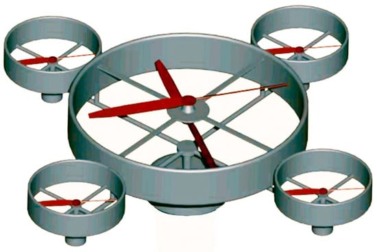
Figure 1.
The layout of the modified UAV [54].
The motion principle of the modified UAV refers to the way in which the UAV is able to move or fly through the air. The flight dynamics are crucial for the safe and efficient operation of the aircraft. It determines how the UAV moves through the air, including its speed, altitude, and direction. Understanding and controlling the motion principle is essential for navigation, maneuverability, and stability, and it is a key aspect of UAV design and control systems. Here, to reduce the gyroscopic effects and prevent the UAV from rotating around its own axis, two pairs of rotors, (1,3) and (2,4), are made to rotate in opposite directions. By adjusting the angular velocity (rotational speed) of the four side rotors, the UAV is able to move in the desired direction. Figure 2 illustrates the principle of motion for the modified UAV. In other words, the figures show how the UAV is able to fly by manipulating the rotational speeds of the side rotors.
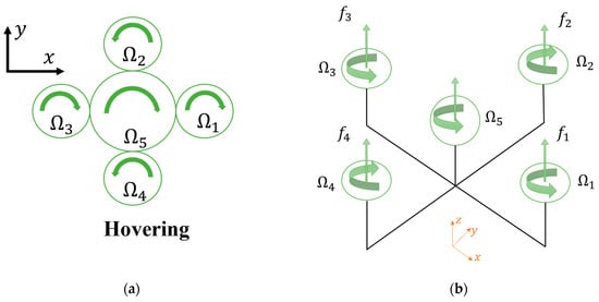
Figure 2.
(a) Scheme and (b) motion principle of the modified UAV [54].
To maintain a stable hover, the rotational speeds of the rotors that are positioned facing each other must be equal. The yaw rotation (rotation about the z-axis) is achieved by adjusting the speeds of each pair of facing rotors. Additionally, changing the speeds of all four rotors together will cause the UAV to move vertically, either upwards or downwards, along the z-axis. By altering the rotational speed of rotors 2 and 4 in opposite directions, the UAV will roll or rotate about the x-axis. Similarly, by adjusting the speeds of rotors 1 and 3 in opposite directions, the UAV will pitch or rotate about the y-axis. These rotations allow the UAV to change its orientation and move in different directions.
Based on the dynamic of the system depicted, the following equations are provided by force and torques on the vehicle’s body:
where indicates the force applying to the body along the z-axis. Additionally, , and denote the torques generated by the rotors that cause the UAV to rotate around the -axis, -axis, and -axis. denotes rotor angular velocity where represents the rotor number (). Furthermore, the thrust force produced by each rotor is represented by (). The thrust and drag factors are represented by and , respectively [54]. Based on the frame system shown in Figure 2, the modified UAV’s translational dynamics, which shows how it moves in relation to a fixed reference frame, are described as follows:
where is the total UAV’s mass, and the acceleration of the center of mass is denoted by . The air friction coefficient that affects the translational motion of the UAV is represented by . This coefficient measures the amount of resistance or drag that the air exerts on the UAV as it moves through it. Additionally, variables and represent the roll, pitch, and yaw angles, respectively. These angles describe the orientation of the UAV’s body in relation to a fixed reference frame. The relationship between the Euler rates (the rates at which the Euler angles change) and the angular body rates (the rates at which the orientation of the UAV’s body changes) is expressed as follows:
Additionaly, the rotational dynamics of modified UAVs are given by:
In this equation, H represents the angular momentum of the UAV, represents the distance between the center of mass and each particle, represents the moment of inertia, and represents the rotor inertia. The air friction coefficient that affects the rotational motion of the UAV is represented by . Furthermore, parameters and are provided by:
To derive the equations of motion, the aerodynamic effects are treated as a disturbance, and it is assumed that the Euler angles are relatively small. Under these assumptions, the rate of change of the Euler angles and the angular velocity of the UAV in the body coordinate system are equal, meaning that:
where p, q, and w are the angular velocity components around the x-axis, y-axis, and z-axis, respectively. Based on the assumption that the Euler angles are small, the equation of motion for the UAV is described as follows:
3. Neural Network Estimator and Problem Formulation
Herein, an overview of the radial basis function (RBF) neural network estimator is provided, followed by the presentation of the problem formulation for the control scheme.
3.1. RBF Neural Network Estimator
An RBF neural network estimator is a type of neural network that is used for approximating functions or making predictions. It is composed of three layers: an input layer, a hidden layer, and an output layer. The hidden layer consists of a number of “radial basis functions”, which are centered at different points and have a certain width or spread. These functions are used to transform the input data into a higher-dimensional space, where it becomes easier to separate or classify. The output layer then combines the outputs of the hidden layer using linear combinations to produce the final output. RBF neural networks are particularly useful for tasks that involve interpolation or extrapolation, and they have been applied to a wide range of fields, including control systems, pattern recognition, and function approximation. The structure of the RBF neural network estimator is shown in Figure 3, where the output of the estimator, denoted as , is calculated as follows:
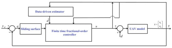
Figure 3.
Block diagram of data-driven-based TSMC for UAV model.
In this equation, represents the ideal constant weight of the RBF, which is used to adjust the strength or importance of each function in the hidden layer. The RBF of the hidden nodes is represented by . m and denote the hidden nodes’ and outputs’ numbers, respectively. represents the inputs’ number, and represents the width value of the basis function, which determines the spread or influence of the function. is the input vector for the RBF, which consists of the input data for the network. represents the bounded RBF approximation error, which measures the difference between the output of the network and the true value. is the center of the basis function, which determines its position in the input space [39].
3.2. Problem Formulation
The general form of the equation that describes the behavior of a nonlinear system can be expressed as follows:
In this equation, represents the state vector of the system. is the uncertain function of the system, which is bounded by an unknown positive constant , such that . represents the constrained control input or the input signal that is applied to the system in order to control its behavior. Furthermore, the external disturbance acting on the system is bound by ε, such that . This disturbance includes any part of the control signal that exceeds the control bounds ()) and cannot be applied to the system. It is important to consider the effect of this disturbance on the system’s behavior. Given a desired trajectory , the tracking error and its function can be defined as follows:
In this equation, are positive constants that are chosen by the user. The time derivative of the error function (11) is provided by:
in which .
4. Control Design
The general state space equation of a nonlinear system affected by disturbance is provided by
To establish the stability of the error system and the ability of the disturbance observer and terminal sliding mode control to track disturbances over a finite time period, the following lemma and theorem are utilized.
Lemma 1 ([32]).
Let be a positive definite function that is continuous. It is proven that converges to its equilibrium point in the finite time
where , and if the following inequality is hold
Additionally, in order to develop the finite-time sliding mode tracking controller, the following sliding surfaces are established.
Using a recursive technique, the jth-order derivative of is calculated as:
By taking into account (15) and (17), the following equation is derived:
where In which, denotes the fractional derivative with fractional order q. We add this term in the sliding surface and accordingly to the control signal to take into account the memory effects uncertainties and unknown function of the system. In other words, the inclusion of a fractional-order derivative term in the sliding surface allows for the control signal to take into account the effects of memory and non-local properties in the system. These effects can cause uncertainties and unknown functions in the system, which can make it difficult to control the system with traditional integer-order derivatives. Furthermore, by including the fractional-order derivative term in the sliding surface, the control signal can more accurately account for these uncertainties and unknown functions. This allows for more precise control of the system, even in the presence of these uncertainties and unknowns. This is because fractional-order derivatives are able to more accurately represent the dynamics of the system and account for the memory effects and non-local properties that can cause these uncertainties and unknowns. Additionally, the fractional-order derivative term in the sliding surface allows for the control signal to be more robust to uncertainties and unknown functions in the system. This improves the overall performance of the control system, as it is able to respond more effectively to changes in the system dynamics and account for the effects of memory and non-local properties.
It is worth mentioning that these advantages come at the cost of mathematical complexity and additional computational requirements. Therefore, the design of a fractional-order controller is more challenging and might require specialized methods and tools. In what follows, the design of this controller is delineated.
As per (13) and (18), the derivative of is represented as follows:
Finally, the data-driven-based terminal sliding mode tracking control signal is provided by:
where and are positive scalar parameters that are used to adjust the performance of the control system are positive parameters. In addition, must be greater than the absolute value of (). In the inputs of the neural network are sliding errors ( and the output of the neural network, represented as , is then combined with the control signal. This combination allows the neural network to learn the inherent behavior of the system and provide additional control signals when necessary to drive the system toward the desired behavior. The use of a neural network to generate the control signal allows for the control method to be highly flexible and adaptive to changing conditions or variations in the system. Additionally, the error of the weight estimation is defined as
The equation that governs the adaptation of the weights of the neural network controller is presented as follows:
where is a positive design parameter.
Proof.
By substituting (20) into (19) and taking into account that = , the following equation is obtained:
By taking into account (20), the following result is derived:
We can assume the Lyapunov function candidate to be:
Considering Equation (23), the derivative of the Lyapunov function with respect to time can be obtained.
Additionally, it is known that and
which leads to
Using Lemma 1 and Equation (27) as theoretical foundations, it can be deduced that when using the disturbance–observer-based terminal sliding mode tracking controller, the closed-loop system signals will reach a stable state within a specific timeframe. □
Figure 4 illustrates the data-driven -based finite time fractional-order controller process. It uses the data-driven observer’s output to estimate all uncertainties and suppress their effects. Uncertain parameters exist in real-world applications, and modeling of the system cannot consider all of them, which is why a robust and intelligent controller is designed. The data-driven-based disturbance observer is proposed to overcome the lack of accuracy due to uncertainty.

Figure 4.
The layout of an RBF neural network.
5. Simulation Results
The following states are defined for the UAV:
Without limiting the generality, the mathematical representation of the UAV’s behavior, Equation (7), is expressed in the state-space form as:
where
where, in accordance with Equation (7), , and . Furthermore, and are written as
The UAV system has six degrees of freedom, while the system has only four control inputs, making it an underactuated system. To overcome this issue, this paper defines virtual position control inputs, and . These virtual control inputs are used to produce the desired roll and pitch angles by tracking the errors of positions x and y. This approach is used to tackle the underactuated problem in the UAV system, which allows for better control of the UAV by providing additional control inputs that are derived from the system’s existing states. This improves the overall performance of the UAV by allowing it to respond more accurately to changes in the system dynamics and external disturbances. As a result, by defining these two virtual control inputs, the UAV’s flight dynamics can be reformulated as follows:
The initial conditions for the system are defined as zero for all states. The desired roll and pitch angles, and , are chosen based on the virtual control inputs, which are calculated as and . Additionally, the parameters of the dynamic model of the modified UAV are listed in Table 1 for reference.

Table 1.
The parameters of the modified UAV.
5.1. Control of UAV with Uncertain Parameters
To evaluate the effectiveness of the controller, the following uncertainties were considered for the parameters of the system.
in which these uncertain and time-varying parameters are considered for all numerical simulations. We consider the following complex a desired path for the system to follow:
MATLAB 2021-a was used for numerical simulations. Figure 5 shows the state of the system over time and how it reaches the desired values quickly. The goal of this figure is to show the proposed control scheme’s efficiency in achieving the desired state. It can be observed that the system reaches the desired values quickly, indicating the control method’s ability to stabilize the system effectively. Figure 6 and Figure 7 provide more information about the control inputs and rotor speeds, respectively. Figure 6 illustrates the control inputs obtained through the proposed control method, which were constrained. Figure 7, on the other hand, presents the speed of each rotor, which is a critical measurement to assess the system’s performance.
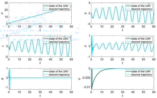
Figure 5.
Time history of system states under proposed control technique.
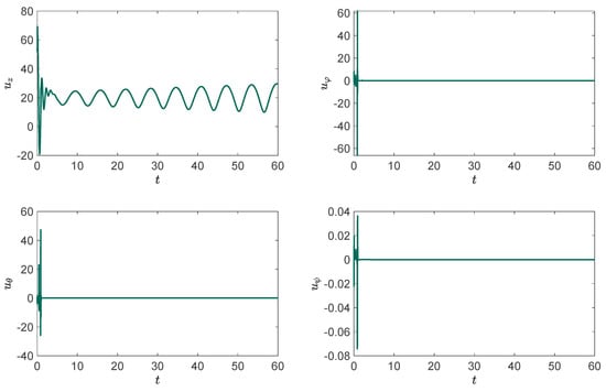
Figure 6.
Control signals obtained based on the proposed control technique.
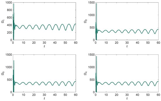
Figure 7.
Rotor’s speed under the proposed control plan.
In addition to what was stated before, Figure 8 provides a detailed representation of the system’s dynamic behavior. The three-dimensional phase plot allows for a better understanding of how the system behaves in terms of its position and velocity. This type of representation is particularly useful in visualizing the system’s trajectory over time and the impact of the disturbances and limitations on the system’s performance. As can be seen in the figure, the proposed control scheme guides the system to follow the desired trajectory, despite the presence of unknown external disturbances and control input limitations. This indicates that the proposed control method is robust and able to effectively stabilize the system in the face of these challenges. Furthermore, the proposed control scheme is able to guide the system to follow the desired path closely, which demonstrates the control method’s high precision and accuracy. Overall, Figure 8 provides a clear visual representation of the proposed control scheme’s ability to effectively stabilize the system. The three-dimensional phase plot allows for a detailed understanding of how the system is behaving, and the results demonstrate that the proposed control method is robust, precise, and able to effectively stabilize the system in the presence of unknown external disturbances and control input limitations.
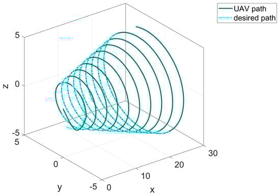
Figure 8.
Three-dimensional phase plot illustrating the trajectory of the system under the proposed control technique.
5.2. Comparison of Results
Real-world systems often exhibit uncertain dynamics that can be characterized by fractional-order functions. To address this type of uncertainty, our proposed controller is designed to be robust and capable of handling such disturbances. To evaluate the performance of the controller under such conditions, we analyze the system’s behavior in the presence of a fractional-order external disturbance. The following disturbance is applied to the system:
We subject the system to an external disturbance that varies over time according to the fractional order Equation (34), with Additionally, we compare the performance of the proposed controller to that of an integer order controller. The integer order controller is similar to the proposed controller but does not include the fractional order term (), as shown in Equation (20). The control signal of the integer order controller is determined as follows:
The sliding surface used in this controller is identical to the signal used in the proposed controller, and it also includes a neural network estimator.
Figure 9 illustrates the system state’s time history under both the proposed control technique and the integer order controller. While the neural network has significantly improved the performance of the integer order controller, its accuracy is not perfect due to the fractional nature of the external disturbance. In contrast, the proposed controller is able to easily handle the disturbance and accurately follow the desired trajectory, as evidenced by the and responses in Figure 9. Further information about the control inputs and rotor speeds can be found in Figure 10 and Figure 11, respectively. Notably, the integer order controller exhibits several jumps in rotor speed and control input, which can limit its practical applications. Therefore, the proposed controller is preferred for its superior performance and a wider range of potential applications.
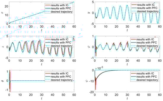
Figure 9.
Comparison of system state time history between proposed fractional order controller (PFC) and integer order controller (IC).
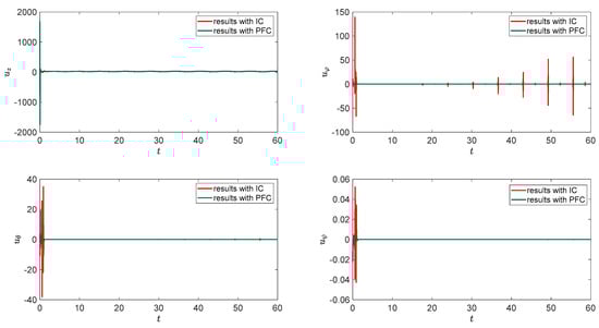
Figure 10.
Comparison of control signals between proposed fractional order controller (PFC) and integer order controller (IC).

Figure 11.
Comparison of rotor speeds between proposed fractional order controller (PFC) and integer order controller (IC).
Figure 12 presents a three-dimensional phase plot that clearly shows the superior performance of the proposed controller compared to its integer counterpart in terms of both accuracy and robustness. The proposed controller is able to effectively handle the external disturbance, resulting in a trajectory that more closely matches the desired path than that of the integer controller. This further emphasizes the effectiveness of the proposed controller and its potential for real-world applications.

Figure 12.
Comparison of three-dimensional phase plot between proposed fractional order controller (PFC) and integer order controller (IC).
It is worth noting that the proposed controller has demonstrated remarkable robustness in handling the fractional nature of the external disturbance, as evidenced by its ability to accurately follow the desired trajectory with a high degree of precision. This robustness is a key advantage of the proposed controller and highlights its potential for addressing uncertainties and disturbances in practical applications.
The numerical results obtained in our study provide clear confirmation of the robustness of our proposed controller when accounting for the memory effect of fractional calculus. Furthermore, the comparison to the integer controller sheds light on the importance of this type of controller which, in addition to the intelligent estimator, is enhanced by fractional factors, suggesting potential avenues for enhancing system performance in uncertain environments.
6. Conclusions
We proposed a new approach to control the tracking of a modified UAV through data-driven fractional-order control. Our method includes extracting the dynamic model of the UAV and providing its state-space equations. The control scheme is designed to handle the uncertainties and disturbances that are typical in UAV systems by incorporating a neural network observer. This observer uses data from the system to estimate the uncertain dynamics of the system and provide a more accurate representation of the system’s behavior. We also used a finite-time and fractional-order control scheme to reduce the impact of these uncertainties. The fractional-order terms in the sliding surface and control input improve the performance of the system in dealing with a wide range of uncertainties which the system will encounter since it can better capture the memory effects. Furthermore, by applying the Lyapunov theorem, we have ensured the finite-time convergence of the system. To conclude, the proposed control technique has been demonstrated to have excellent performance through numerical results. The proposed control technique for a modified UAV could have practical applications in a number of fields, including aerial photography, search and rescue operations, and remote sensing. For example, in aerial photography, the proposed control scheme could provide improved stability and accuracy in capturing aerial images. In search and rescue operations, the control scheme could help a UAV navigate through challenging environments and provide real-time data and images for rescue teams. In remote sensing, the control scheme could help a UAV accurately collect data from remote areas and provide improved accuracy in data analysis and interpretation. However, as a future research direction, one can study the robustness of the proposed control scheme against faults and also investigate the use of other types of neural networks to improve the closed-loop system’s performance. This could include using other types of neural networks, such as recurrent neural networks (RNNs), which have been shown to be effective in a variety of control applications.
Author Contributions
Conceptualization, F.W.A., H.J., Q.Y., M.S.A.-z. and A.S.A.; Methodology, F.W.A., H.J., Q.Y., M.S.A.-z. and A.S.A.; Software, F.W.A., H.J., Q.Y., M.S.A.-z. and A.S.A.; Validation, F.W.A., H.J., Q.Y., M.S.A.-z. and A.S.A.; Formal analysis, F.W.A., H.J., Q.Y., M.S.A.-z. and A.S.A.; Investigation, F.W.A., H.J., Q.Y., M.S.A.-z. and A.S.A.; Resources, F.W.A., H.J., Q.Y., M.S.A.-z. and A.S.A.; Data curation, F.W.A., H.J., Q.Y., M.S.A.-z. and A.S.A.; Writing—original draft, F.W.A., H.J., Q.Y., M.S.A.-z. and A.S.A.; Writing—review & editing, F.W.A., H.J., Q.Y., M.S.A.-z. and A.S.A.; Visualization, F.W.A., H.J., Q.Y., M.S.A.-z. and A.S.A.; Supervision, F.W.A., H.J., Q.Y., M.S.A.-z. and A.S.A.; Project administration, F.W.A., H.J., Q.Y., M.S.A.-z. and A.S.A.; Funding acquisition, F.W.A., H.J., Q.Y., M.S.A.-z. and A.S.A. All authors have read and agreed to the published version of the manuscript.
Funding
This study is supported by the Deanship of Scientific Research at King Faisal University under Grant No. 17122015.
Institutional Review Board Statement
Not applicable.
Informed Consent Statement
Not applicable.
Data Availability Statement
Not applicable.
Conflicts of Interest
The authors declare no conflict of interest.
References
- Paw, Y.C. Synthesis and Validation of Flight Control for UAV; University of Minnesota: Minneapolis, MN, USA, 2009; ISBN 1109558449. [Google Scholar]
- Chen, H.; Wang, X.; Li, Y. A Survey of Autonomous Control for UAV. In Proceedings of the 2009 International Conference on Artificial Intelligence and Computational Intelligence, Shanghai, China, 7–8 November 2009; Volume 2, pp. 267–271. [Google Scholar]
- Zhao, J.; Gao, F.; Ding, G.; Zhang, T.; Jia, W.; Nallanathan, A. Integrating Communications and Control for UAV Systems: Opportunities and Challenges. IEEE Access 2018, 6, 67519–67527. [Google Scholar] [CrossRef]
- Kurdel, P.; Češkovič, M.; Gecejová, N.; Adamčík, F.; Gamcová, M. Local Control of Unmanned Air Vehicles in the Mountain Area. Drones 2022, 6, 54. [Google Scholar] [CrossRef]
- Ouyang, Q.; Wu, Z.; Cong, Y.; Wang, Z. Formation Control of Unmanned Aerial Vehicle Swarms: A Comprehensive Review. Asian J. Control. 2022, 25, 570–593. [Google Scholar] [CrossRef]
- Yousefpour, A.; Yasami, A.; Beigi, A.; Liu, J. On the Development of an Intelligent Controller for Neural Networks: A Type 2 Fuzzy and Chatter-Free Approach for Variable-Order Fractional Cases. Eur. Phys. J. Spec. Top. 2022, 231, 2045–2057. [Google Scholar] [CrossRef]
- Hilfer, R. Applications of Fractional Calculus in Physics; World Scientific: Singapore, 2000; ISBN 9814496200. [Google Scholar]
- Machado, J.T.; Kiryakova, V.; Mainardi, F. Recent History of Fractional Calculus. Commun. Nonlinear. Sci. Numer. Simul. 2011, 16, 1140–1153. [Google Scholar] [CrossRef]
- Sun, H.; Zhang, Y.; Baleanu, D.; Chen, W.; Chen, Y. A New Collection of Real World Applications of Fractional Calculus in Science and Engineering. Commun. Nonlinear. Sci. Numer. Simul. 2018, 64, 213–231. [Google Scholar] [CrossRef]
- Xu, C.; Mu, D.; Liu, Z.; Pang, Y.; Liao, M.; Li, P.; Yao, L.; Qin, Q. Comparative Exploration on Bifurcation Behavior for Integer-Order and Fractional-Order Delayed BAM Neural Networks. Nonlinear. Anal. Model. Control. 2022, 27, 1–24. [Google Scholar] [CrossRef]
- Atangana, A. Application of Fractional Calculus to Epidemiology. Fract. Dyn. 2015, 2015, 174–190. [Google Scholar]
- Tenreiro Machado, J.A.; Silva, M.F.; Barbosa, R.S.; Jesus, I.S.; Reis, C.M.; Marcos, M.G.; Galhano, A.F. Some Applications of Fractional Calculus in Engineering. Math. Probl. Eng. 2010, 2010, 639801. [Google Scholar] [CrossRef]
- Kulish, V.; Lage, J.L. Application of Fractional Calculus to Fluid Mechanics. J. Fluids. Eng. 2002, 124, 803–806. [Google Scholar] [CrossRef]
- Tarasov, V.E. Mathematical Economics: Application of Fractional Calculus. Mathematics 2020, 8, 660. [Google Scholar] [CrossRef]
- Victor, S.; Duhé, J.-F.; Melchior, P.; Abdelmounen, Y.; Roubertie, F. Long-Memory Recursive Prediction Error Method for Identification of Continuous-Time Fractional Models. Nonlinear Dyn. 2022, 110, 635–648. [Google Scholar] [CrossRef]
- Jallouli-Khlif, R.; Maalej, B.; Melchior, P.; Derbel, N. Control of Prosthetic Hand Based on Input Shaping Combined to Fractional PI Controller. In Proceedings of the 2021 9th International Conference on Systems and Control (ICSC), Caen, France, 24–26 November 2021; pp. 449–454. [Google Scholar]
- Yousfi, N.; Derbel, N.; Melchior, P.; Almalki, H. Robust Motion Control Using Combined Centralized Non-Integer Pre-Filter of Type FBLFD and Fractional Order PDμ Controller. Int. J. Innov. Technol. Explor. Eng. 2019, 9, 3463. [Google Scholar] [CrossRef]
- Rammal, R.; Airimitoaie, T.-B.; Melchior, P.; Cazaurang, F. Flatness-Based Fault Detection and Isolation for Fractional Order Linear Flat Systems. 2022. Available online: https://hal.science/hal-03601386/file/Fractiona_FDI_Final_version.pdf (accessed on 8 March 2022).
- Rammal, R.; Airimitoaie, T.-B.; Melchior, P.; Cazaurang, F. Unimodular Completion for Computation of Fractionally Flat Outputs for Linear Fractionally Flat Systems. IFAC-PapersOnLine 2020, 53, 4415–4420. [Google Scholar] [CrossRef]
- Humphreys, P.C.; Raposo, D.; Pohlen, T.; Thornton, G.; Chhaparia, R.; Muldal, A.; Abramson, J.; Georgiev, P.; Santoro, A.; Lillicrap, T. A Data-Driven Approach for Learning to Control Computers. In Proceedings of the International Conference on Machine Learning, PMLR, Seoul, Republic of Korea, 17–23 July 2022; pp. 9466–9482. [Google Scholar]
- Wen, L.; Li, X.; Gao, L.; Zhang, Y. A New Convolutional Neural Network-Based Data-Driven Fault Diagnosis Method. IEEE Trans. Ind. Electron. 2017, 65, 5990–5998. [Google Scholar] [CrossRef]
- Kisvari, A.; Lin, Z.; Liu, X. Wind Power Forecasting–A Data-Driven Method along with Gated Recurrent Neural Network. Renew Energy 2021, 163, 1895–1909. [Google Scholar] [CrossRef]
- Xia, M.; Zheng, X.; Imran, M.; Shoaib, M. Data-Driven Prognosis Method Using Hybrid Deep Recurrent Neural Network. Appl. Soft. Comput. 2020, 93, 106351. [Google Scholar] [CrossRef]
- Sun, T.-C.; Yousefpour, A.; Karaca, Y.; Alassafi, M.O.; Ahmad, A.M.; Li, Y.-M. Dynamical Investigation and Distributed Consensus Tracking Control of a Variable-Order Fractional Supply Chain Network Using a Multi-Agent Neural Network-Based Control Method. Fractals 2022, 30, 1–13. [Google Scholar] [CrossRef]
- Xu, C.; Mu, D.; Liu, Z.; Pang, Y.; Liao, M.; Aouiti, C. New Insight into Bifurcation of Fractional-Order 4D Neural Networks Incorporating Two Different Time Delays. Commun. Nonlinear. Sci. Numer. Simul. 2023, 118, 107043. [Google Scholar] [CrossRef]
- Huang, C.; Wang, J.; Chen, X.; Cao, J. Bifurcations in a Fractional-Order BAM Neural Network with Four Different Delays. Neural Netw. 2021, 141, 344–354. [Google Scholar] [CrossRef]
- Huang, C.; Tang, J.; Niu, Y.; Cao, J. Enhanced Bifurcation Results for a Delayed Fractional Neural Network with Heterogeneous Orders. Phys. A Stat. Mech. Its Appl. 2019, 526, 121014. [Google Scholar] [CrossRef]
- Yousefpour, A.; Jahanshahi, H.; Castillo, O. Application of Variable-Order Fractional Calculus in Neural Networks: Where Do We Stand? Eur. Phys. J. Spec. Top. 2022, 231, 1753–1756. [Google Scholar] [CrossRef]
- Yasami, A.; Beigi, A.; Yousefpour, A. Application of Long Short-Term Memory Neural Network and Optimal Control to Variable-Order Fractional Model of HIV/AIDS. Eur. Phys. J. Spec. Top. 2022, 231, 1875–1884. [Google Scholar] [CrossRef]
- Jahanshahi, H.; Yao, Q.; Khan, M.I.; Moroz, I. Unified Neural Output-Constrained Control for Space Manipulator Using Tan-Type Barrier Lyapunov Function. Adv. Space Res. 2022; in press. [Google Scholar]
- Li, Y.; Yang, T.; Tong, S. Adaptive Neural Networks Finite-Time Optimal Control for a Class of Nonlinear Systems. IEEE Trans. Neural Netw. Learn Syst. 2019, 31, 4451–4460. [Google Scholar] [CrossRef] [PubMed]
- Ren, Y.M.; Alhajeri, M.S.; Luo, J.; Chen, S.; Abdullah, F.; Wu, Z.; Christofides, P.D. A Tutorial Review of Neural Network Modeling Approaches for Model Predictive Control. Comput. Chem. Eng. 2022, 165, 107956. [Google Scholar] [CrossRef]
- Alsaade, F.W.; Jahanshahi, H.; Yao, Q.; Al-zahrani, M.S.; Alzahrani, A.S. A New Neural Network-Based Optimal Mixed H2/H∞ Control for a Modified Unmanned Aerial Vehicle Subject to Control Input Constraints. Adv. Space Res. 2022; in press. [Google Scholar]
- Shtessel, Y.; Edwards, C.; Fridman, L.; Levant, A. Sliding Mode Control and Observation; Springer: Berlin/Heidelberg, Germany, 2014; Volume 10. [Google Scholar]
- Hu, J.; Zhang, H.; Liu, H.; Yu, X. A Survey on Sliding Mode Control for Networked Control Systems. Int. J. Syst. Sci. 2021, 52, 1129–1147. [Google Scholar] [CrossRef]
- Jahanshahi, H. Smooth Control of HIV/AIDS Infection Using a Robust Adaptive Scheme with Decoupled Sliding Mode Supervision. Eur. Phys. J. Spec. Top. 2018, 227, 707–718. [Google Scholar] [CrossRef]
- Yao, Q.; Jahanshahi, H.; Moroz, I.; Bekiros, S.; Alassafi, M.O. Indirect Neural-Based Finite-Time Integral Sliding Mode Control for Trajectory Tracking Guidance of Mars Entry Vehicle. Adv. Space Res. 2022; in press. [Google Scholar]
- Alsubaie, H.; Yousefpour, A.; Alotaibi, A.; Alotaibi, N.D.; Jahanshahi, H. Fault-Tolerant Terminal Sliding Mode Control with Disturbance Observer for Vibration Suppression in Non-Local Strain Gradient Nano-Beams. Mathematics 2023, 11, 789. [Google Scholar] [CrossRef]
- Yu, X.; Feng, Y.; Man, Z. Terminal Sliding Mode Control–an Overview. IEEE Open J. Ind. Electron. Soc. 2020, 2, 36–52. [Google Scholar] [CrossRef]
- Yousefpour, A.; Jahanshahi, H.; Munoz-Pacheco, J.M.; Bekiros, S.; Wei, Z. A Fractional-Order Hyper-Chaotic Economic System with Transient Chaos. Chaos Solitons Fractals 2020, 130, 109400. [Google Scholar] [CrossRef]
- Jahanshahi, H.; Yousefpour, A.; Munoz-Pacheco, J.M.; Kacar, S.; Pham, V.-T.; Alsaadi, F.E. A New Fractional-Order Hyperchaotic Memristor Oscillator: Dynamic Analysis, Robust Adaptive Synchronization, and Its Application to Voice Encryption. Appl. Math. Comput. 2020, 383, 125310. [Google Scholar] [CrossRef]
- Chen, S.-B.; Beigi, A.; Yousefpour, A.; Rajaee, F.; Jahanshahi, H.; Bekiros, S.; Martínez, R.A.; Chu, Y. Recurrent Neural Network-Based Robust Nonsingular Sliding Mode Control with Input Saturation for a Non-Holonomic Spherical Robot. IEEE Access 2020, 8, 188441–188453. [Google Scholar] [CrossRef]
- Eskandari, B.; Yousefpour, A.; Ayati, M.; Kyyra, J.; Pouresmaeil, E. Finite-Time Disturbance-Observer-Based Integral Terminal Sliding Mode Controller for Three-Phase Synchronous Rectifier. IEEE Access 2020, 8, 152116–152130. [Google Scholar] [CrossRef]
- Yousefpour, A.; Haji Hosseinloo, A.; Reza Hairi Yazdi, M.; Bahrami, A. Disturbance Observer–Based Terminal Sliding Mode Control for Effective Performance of a Nonlinear Vibration Energy Harvester. J. Intell. Mater. Syst. Struct. 2020, 31, 1495–1510. [Google Scholar] [CrossRef]
- Sun, C.; Liu, M.; Liu, C.; Feng, X.; Wu, H. An Industrial Quadrotor Uav Control Method Based on Fuzzy Adaptive Linear Active Disturbance Rejection Control. Electronics 2021, 10, 376. [Google Scholar] [CrossRef]
- Chen, X.; Wang, L. Cascaded Model Predictive Control of a Quadrotor UAV. In Proceedings of the 2013 Australian Control Conference, Fremantle, WA, Australia, 4–5 November 2013; pp. 354–359. [Google Scholar]
- ud Din, A.F.; Mir, I.; Gul, F.; Mir, S.; Saeed, N.; Althobaiti, T.; Abbas, S.M.; Abualigah, L. Deep Reinforcement Learning for Integrated Non-Linear Control of Autonomous UAVs. Processes 2022, 10, 1307. [Google Scholar] [CrossRef]
- Whitehead, B.; Bieniawski, S. Model Reference Adaptive Control of a Quadrotor UAV. In Proceedings of the AIAA Guidance, Navigation, and Control Conference, Toronto, ON, Canada, 2–5 August 2010; p. 8148. [Google Scholar]
- Dydek, Z.T.; Annaswamy, A.M.; Lavretsky, E. Adaptive Control of Quadrotor UAVs: A Design Trade Study with Flight Evaluations. IEEE Trans. Control Syst. Technol. 2012, 21, 1400–1406. [Google Scholar] [CrossRef]
- Min, B.-C.; Hong, J.-H.; Matson, E.T. Adaptive Robust Control (ARC) for an Altitude Control of a Quadrotor Type UAV Carrying an Unknown Payloads. In Proceedings of the 2011 11th International Conference on Control, Automation and Systems, Gyeonggi-do, Republic of Korea, 26–29 October 2011; pp. 1147–1151. [Google Scholar]
- Raffo, G.V.; de Almeida, M.M. Nonlinear Robust Control of a Quadrotor UAV for Load Transportation with Swing Improvement. In Proceedings of the 2016 American Control Conference (ACC), Boston, MA, USA, 6–8 July 2016; pp. 3156–3162. [Google Scholar]
- Santoso, F.; Liu, M.; Egan, G. Linear Quadratic Optimal Control Synthesis for a Uav. In Proceedings of the 12th Australian International Aerospace Congress, AIAC12, Melbourne, Australia, 12–16 May 2007. [Google Scholar]
- Satici, A.C.; Poonawala, H.; Spong, M.W. Robust Optimal Control of Quadrotor UAVs. IEEE Access 2013, 1, 79–93. [Google Scholar] [CrossRef]
- Tofigh, M.A.L.I.; Mahjoob, M.; Ayati, M. Feedback linearization and back stepping controller aimed at position tracking for a novel five-rotor uav. Modares Mech. Eng. 2015, 15, 247–254. [Google Scholar]


Disclaimer/Publisher’s Note: The statements, opinions and data contained in all publications are solely those of the individual author(s) and contributor(s) and not of MDPI and/or the editor(s). MDPI and/or the editor(s) disclaim responsibility for any injury to people or property resulting from any ideas, methods, instructions or products referred to in the content. |
© 2023 by the authors. Licensee MDPI, Basel, Switzerland. This article is an open access article distributed under the terms and conditions of the Creative Commons Attribution (CC BY) license (https://creativecommons.org/licenses/by/4.0/).