Studying and Simulating the Fractional COVID-19 Model Using an Efficient Spectral Collocation Approach

Abstract

We give a theoretical and numerical analysis of a coronavirus (COVID-19) infection model in this research. A mathematical model of this system is provided, based on a collection of fractional differential equations (in the Caputo sense). Initially, a rough approximation formula was created for the fractional derivative of $t^p$. Here, the third-kind Chebyshev approximations of the spectral collocation method (SCM) were used. To identify the unknown coefficients of the approximate solution, the proposed problem was transformed into a system of algebraic equations, which was then transformed into a restricted optimization problem. To evaluate the effectiveness and accuracy of the suggested scheme, the residual error function was computed. The objective of this research was to halt the global spread of a disease. A susceptible person may be moved immediately into the confined class after being initially quarantined or an exposed person may be transferred to one of the infected classes. The researchers adopted this strategy and considered both asymptomatic and symptomatic infected patients. Results acquired with the achieved results were contrasted with those obtained using the generalized Runge-Kutta method.

1. Introduction

There are many models that are used to describe many phenomena in biology and COVID-19, such as [1,2,3,4]. To understand how the pandemic spread, its effects, how it could have been prevented and controlled, and the transmission of disease, as well as the outcomes of preventive measures such as hand washing with a disinfecting hand sanitizer, increasing the distance between people, and wearing face masks, researchers have been using and developing mathematical models [5,6,7,8]. In [9], the early stages of the outbreak of COVID-19 in Nigeria was examined and assessed by the authors. Good research on preventive and therapeutic strategies to curb the epidemic were provided by researchers from a range of fields, with encouraging outcomes. Nevertheless, the most current models need to be examined more thoroughly to make a valid and satisfactory judgment [10,11,12,13].

All of the models described in the preceding investigations usually used known derivatives [14]. These differential operators have memory qualities, allowing them to be utilized to demonstrate a wide range of scientific phenomena and facts involving dynamics [15,16,17]. The concept of fractional differential equations (FDEs) in general, and ordinary differential equations (ODEs) in particular, has gained a lot of interest due to its wide-ranging improvements to and numerous applications in several disciplines [18,19]. Recent literature [20] has introduced local fractional derivative operators. These derivatives, which are local in nature, are helpful for researching the fractional differentiability characteristics of extremely irregular and nowhere-differentiable functions. Existing ideas on local fractional derivatives have some strong connections to the standard derivative function. In actuality, the first-order derivative of a function multiplied by a continuous function is the $\alpha$-derivative of that function. In addition, the majority of $\alpha$-differentiation results are trivially inferable from the conventional ones. Hence, local fractional calculus is a fascinating concept that merits more study.

Approximate solutions for FDEs were developed using SCMs [21,22,23]. The main advantage of these methods is that they can generate exact findings with fewer degrees of freedom. The Chebyshev polynomials were used as orthogonal polynomials to approximate functions in the interval $[-1,1]$. These polynomials are crucial to the development of spectral techniques for FDEs [24,25,26] due to the following reasons:

1.

Numerical programs in the suggested technique for managing the study’s model quickly produce Chebyshev coefficients for the solution;

2.

The suggested approach using these polynomials is quicker than the alternatives. Moreover, these polynomials are widely employed and have a wide range of applications due to their favorable function-approximation characteristics;

3.

The suggested approach using these polynomials is an easy-to-use numerical technique with finite and infinite domains for a variety of problems with excellent accuracy and exponential rates of convergence.

This study’s main objective was to offer a theoretical and numerical simulation of the proposed COVID-19 system. The qualitative analysis of the proposed model is presented and concerns the locally asymptotically stable endemic equilibrium point, the locally stable disease-free equilibrium, and the globally asymptotically stable endemic equilibrium. A particular focus was placed on providing a rough formula for the Caputo fractional (CF) derivative with the use of the shifted Chebyshev polynomials. The model was turned into an algebraic system of equations using the suggested method and this approximation of a formula. The system was then stated as a constrained optimization problem, and the problem was then optimized to find the unknown coefficients for the approximate solution. Finally, we gave a numerical simulation of the model under study using the proposed method with different values for the initial values, the various natality rate values, and the distinct values of the fractional derivative. In addition, the residual error function was introduced to estimate the error of the solution. In addition, we compared the solution generated by the proposed method with the generalized Runge-Kutta method of the fourth-order (GRK4).

The following is how the manuscript is organized: The definitions and approximate formula for the CF derivative are presented in Section 2, along with some ideas concerning the newly introduced shifted Chebyshev polynomials. The formulation and qualitative analysis of the model is described in Section 3, where we also look at the stability of the endemic equilibrium point and the invariant region. The solution process for the model being studied is introduced in Section 4 of this article. In Section 5, numerical simulation is also covered. We provide the conclusion and any planned follow-up work in Section 6.

2. Preliminaries and Notations

2.1. Some Definitions of Fractional Derivatives

Definition 1.

The Caputo derivative $D^{\alpha }$ of fractional-order $n-1<\alpha <n$ of a function $\zeta \left(y\right)\in H^1(0,b)$ may be defined as follows:

$$D^{\alpha }\zeta \left(y\right)=\frac{1}{\Gamma (1-\alpha )}{\int }_0^y\frac{{\zeta }^{\left(n\right)}\left(\tau \right)}{{(y-\tau )}^{\alpha }}d\tau ,y>0.$$

(1)

In the following theorem, we give an approximate formula for $t^p$ to use later to derive the main numerical scheme for the model under study.

Theorem 1.

The Caputo derivative of order $n-1<\alpha <n$ of the function $\zeta \left(t\right)=t^p$ with $p\ge n$, ($n=\lceil \alpha \rceil$) is approximated in the interval $[0,b]$ as follows:

$$\begin{array}{cc}\hfill D^{\alpha }{t}^p=& \frac{\Gamma (p+1)}{\Gamma (p+1-\lceil \alpha \rceil )\Gamma (1-\alpha )}\times \frac{h}{3}[G_{\alpha ,p}(t,{\xi }_0)+G_{\alpha ,p}(t,{\xi }_m)\hfill \\ & +4\sum _{k=1,k-odd}^{m-1}{G}_{\alpha ,p}(t,{\xi }_k)+2\sum _{k=2,k-even}^{m-2}{G}_{\alpha ,p}(t,{\xi }_k)].\hfill \end{array}$$

(2)

The domain $[0,b]$ is divided (with the length of each segment being h) into m equal segments:

$$h=\frac{b}{m},G_{\alpha ,p}(t,\xi )={\xi }^{p-\lceil \alpha \rceil }{(t-\xi )}^{-\alpha },{\xi }_k=kh,k=0,1,2,\dots ,m.$$

Proof. 

Using Formula (1) in Definition 1 (CF derivative), we obtain $D^n{t}^p=0,p=0,1,2,\dots ,\lceil \alpha \rceil -1$. Now, for $p\ge \lceil \alpha \rceil$ we have the following:

$$\begin{array}{cc}\hfill D^{\alpha }{t}^p& =\frac{1}{\Gamma (1-\alpha )}{\int }_0^t{D}^n\left({\xi }^p\right){(t-\xi )}^{-\alpha }d\xi =\frac{1}{\Gamma (1-\alpha )}{\int }_0^t\frac{\Gamma (p+1)}{\Gamma (p+1-n)}{\xi }^{p-n}{(t-\xi )}^{-\alpha }d\xi \hfill \\ & =\frac{\Gamma (p+1)}{\Gamma (p+1-n)\Gamma (1-\alpha )}{\int }_0^t{G}_{\alpha ,p}(t,\xi )d\xi .\hfill \end{array}$$

We used Simpson-$\frac{1}{3}$ to evaluate the complicated integral above. We can approximately derive Formula (2) of $D^{\alpha }{t}^p$ as follows:

$$\begin{array}{cc}\hfill D^{\alpha }{t}^p=& \frac{\Gamma (p+1)}{\Gamma (p+1-n)\Gamma (1-\alpha )}\times \frac{h}{3}[G_{\alpha ,p}(t,{\xi }_0)+G_{\alpha ,p}(t,{\xi }_m)\hfill \\ & +4\sum _{k=1,k-odd}^{m-1}{G}_{\alpha ,p}(t,{\xi }_k)+2\sum _{k=2,k-even}^{m-2}{G}_{\alpha ,p}(t,{\xi }_k)].\hfill \end{array}$$

□

For more details on the Caputo derivatives see [27].

2.2. Shifted Chebyshev Polynomial Approximation

The third type of orthogonal Chebyshev polynomial of degree n is generated by the following formula [28]:

$$V_n\left(z\right)=\frac{\cos \left(\right(n+0.5\left)\theta \right)}{\cos \left(0.5\theta \right)},z=\cos \left(\theta \right),0\le \theta \le \pi .$$

This set of polynomials is orthogonal on $[-1,1]$, with respect to the weight function $w\left(z\right)=\sqrt{(1+z)/(1-z)}$, if the following condition is satisfied:

$${\int }_{-1}^{1}w\left(z\right)V_r\left(z\right)V_s\left(z\right)dz=\left\{\begin{array}{cc}0,\hfill & \mathrm{if}r\ne s;\hfill \\ \pi ,\hfill & \mathrm{if}r=s.\hfill \end{array}\right.$$

These polynomials can be constructed directly from the following recurrence formula [29]:

$$V_{n+1}\left(z\right)=2z{V}_n\left(z\right)-V_{n-1}\left(z\right),V_0\left(z\right)=1,V_1\left(z\right)=2z-1,n=1,2,\dots .$$

By using the linear transformation $z=(2/b)t-1$, we can generate the so-called shifted Chebyshev polynomials on $[0,b]$, which are denoted and defined as ${\overline{\mathbb{T}}}_n\left(t\right)=V_n((2/b)t-1)$, where ${\overline{\mathbb{T}}}_0\left(t\right)=1,{\overline{\mathbb{T}}}_1\left(t\right)=(4/b)t-3$. The analytic form is given as follows:

$${\overline{\mathbb{T}}}_n\left(t\right)=\sum _{k=0}^n{(-1)}^k{2}^{2n-2k}\frac{(2n+1)\Gamma (2n-k+1)}{b^{n-k}\Gamma (k+1)\Gamma (2n-2k+2)}{t}^{n-k},n=2,3,\dots .$$

(3)

Note that ${\overline{\mathbb{T}}}_k\left(0\right)={(-1)}^k(2k+1),{\overline{\mathbb{T}}}_k\left(b\right)=1,k=0,1,2\dots .$ The most used of these functions expresses any function $\Omega \left(t\right)\in L_2[0,b]$ as a sum of infinite series as follows:

$$\Omega \left(t\right)=\sum _{\ell =0}^{\infty }{a}_{\ell }{\overline{\mathbb{T}}}_{\ell }\left(t\right),a_{\ell }=\frac{2}{\pi }{\int }_0^b\overline{w}\left(t\right)\Omega \left(t\right){\overline{\mathbb{T}}}_{\ell }\left(t\right)dx,\overline{w}\left(t\right)=\sqrt{\frac{t}{1-t}}.\ell =0,1,\dots .$$

(4)

The series in (4) is cut with the first $(m+1)$-terms of (3) to give the following:

$${\Omega }_m\left(t\right)=\sum _{\ell =0}^m{a}_{\ell }{\overline{\mathbb{T}}}_{\ell }\left(t\right).$$

(5)

In [30], Handan demonstrated the uniform convergence of the shifted Chebyshev expansion (finite series (5)) and generated a formula for the upper bound of the error when approximating the function $\Omega \left(t\right)$ (5).

Additionally, by the use of the expression for the shifted Chebyshev polynomials (5) and a few characteristics of the Caputo fractional (CF) derivative, we can provide a reasonable formula for $D^{\alpha }{\Omega }_i\left(t\right)$ to use later to derive the main numerical scheme for the model under study.

Theorem 2.

The α-order of the CF derivative for the function ${\Omega }_i\left(t\right)$, which is defined in Equation (5), can be evaluated as follows:

$$\begin{array}{cc}\hfill D^{\alpha }{\Omega }_i\left(t\right)& =\sum _{j=\lceil \alpha \rceil }^i{a}_j{\chi }_{i,j,\alpha }[G_{\alpha ,p}(t,{\xi }_0)+G_{\alpha ,p}(t,{\xi }_m)+4\sum _{k=1,k-odd}^{m-1}{G}_{\alpha ,p}(t,{\xi }_k)+2\sum _{k=2,k-even}^{m-2}{G}_{\alpha ,p}(t,{\xi }_k)],\hfill \end{array}$$

(6)

where

$${\chi }_{i,j,\alpha }=\frac{h\Gamma (i-j+1)}{3\Gamma (i-j+1-\lceil \alpha \rceil )}\times \frac{{(-1)}^j(2i+1)4^{i-j}\Gamma (2i-j+1)}{b^{i-j}\Gamma (j+1)\Gamma (2i-2j+2)},G_{\alpha ,p}(t,\xi )={\xi }^{p-\lceil \alpha \rceil }{(t-\xi )}_{p=i-j}^{-\alpha }.$$

Proof. 

By using Theorem 1 we have the following:

$$\begin{array}{cc}\hfill D^{\alpha }{t}^{i-j}=& \frac{\Gamma (i-j+1)}{\Gamma (i-j-\lceil \alpha \rceil +1)}\times \frac{h}{3}[G_{\alpha ,p}(t,{\xi }_0)+G_{\alpha ,p}(t,{\xi }_m)\hfill \\ & +4\sum _{k=1,k-odd}^{m-1}{G}_{\alpha ,p}(t,{\xi }_k)+2\sum _{k=2,k-even}^{m-2}{G}_{\alpha ,p}(t,{\xi }_k)].\hfill \end{array}$$

(7)

The domain $[0,b]$ is divided into m equal segments where each segment has a length of h:

$$h=\frac{b}{m},G_{\alpha ,p}(t,\xi )={\xi }^{p-\lceil \alpha \rceil }{(t-\xi )}_{p=i-j}^{-\alpha },{\xi }_k=kh,k=0,1,2,\dots ,m.$$

Connecting Equations (3), (5), and (7), we can evaluate the CF derivative of the $i^{th}$ degree, ${\Omega }_i\left(t\right)$, as follows:

$$\begin{array}{cc}\hfill D^{\alpha }{\Omega }_i\left(t\right)& =\sum _{j=0}^i\frac{{(-1)}^j(2i+1)4^{i-j}\Gamma (2i-j+1)}{b^{i-j}\Gamma (j+1)\Gamma (2i-2j+2)}{D}^{\alpha }{t}^{i-j}\hfill \\ & =\sum _{j=\lceil \alpha \rceil }^i\frac{\Gamma (i-j+1)}{\Gamma (i-j+1-\lceil \alpha \rceil )}\times \frac{{(-1)}^j(2i+1)4^{i-j}\Gamma (2i-j+1)}{b^{i-j}\Gamma (j+1)\Gamma (2i-2j+2)}\times \frac{h}{3}[G_{\alpha ,p}(t,{\xi }_0)+G_{\alpha ,p}(t,{\xi }_m)\hfill \\ & +4\sum _{k=1,k-odd}^{m-1}{G}_{\alpha ,p}(t,{\xi }_k)+2\sum _{k=2,k-even}^{m-2}{G}_{\alpha ,p}(t,{\xi }_k)].\hfill \end{array}$$

(8)

From this result, we can easily obtain the required formula, Formula (6), and this ends the proof. □

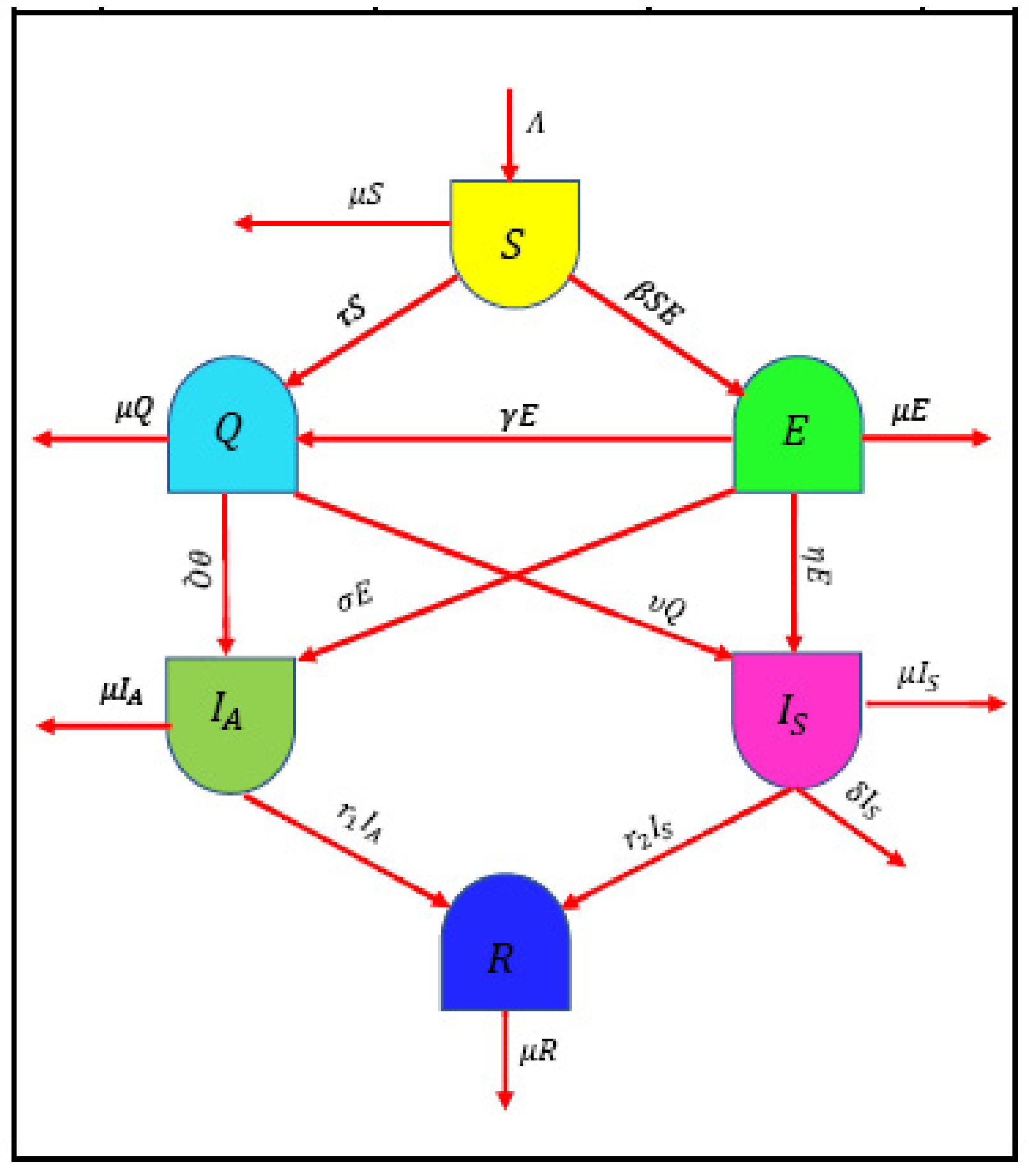
3. The Formulation and Qualitative Analysis of the Model

Let $N\left(t\right)$ be the total number of people. Individuals who are susceptible, exposed, asymptotically infected, symptomatically infected, quarantined, and removed by COVID-19 are denoted as $S\left(t\right)$, $E\left(t\right)$, $I_A\left(t\right)$, $I_S\left(t\right)$, $Q\left(t\right)$, and $R\left(t\right)$, respectively. Taking this into account, the total population is calculated as follows [31]:

$$N\left(t\right)=S\left(t\right)+E\left(t\right)+Q\left(t\right)+I_A\left(t\right)+I_S\left(t\right)+R\left(t\right).$$

A system of ODEs is generated using the schematic diagram in Figure 1 and is described in [31].

This nonlinear system of ODEs can be written as follows:

$$\begin{array}{cc}\hfill & \dot{S}\left(t\right)=\Lambda -(\tau +\mu )S\left(t\right)-\beta S\left(t\right)E\left(t\right),\hfill \\ & \dot{E}\left(t\right)=\beta S\left(t\right)E\left(t\right)-(\gamma +\mu +\eta +\sigma )E\left(t\right),\hfill \\ & \dot{Q}\left(t\right)=\tau S\left(t\right)+\gamma E\left(t\right)-(\mu +v+\theta )Q\left(t\right),\hfill \\ & {\dot{I}}_A\left(t\right)=\sigma E\left(t\right)+\theta Q\left(t\right)-\left(\mu +r_1\right)I_A\left(t\right),\hfill \\ & {\dot{I}}_S\left(t\right)=\eta E\left(t\right)+\upsilon \upsilon Q\left(t\right)-\left(\delta +\mu +r_2\right)I_S\left(t\right),\hfill \\ & \dot{R}\left(t\right)=r_1{I}_A\left(t\right)+r_2{I}_S\left(t\right)-\mu R\left(t\right),\hfill \end{array}$$

(9)

with the initial conditions

$$\begin{array}{cc}\hfill & S\left(0\right)=S_0,E\left(0\right)=E_0,Q\left(0\right)=Q_0,I_A\left(0\right)=I{A}_0,I_S\left(0\right)=I{S}_0,R\left(0\right)=R_0.\hfill \end{array}$$

(10)

All the quantities, $S_0,E_0,Q_0,I{A}_0,I{S}_0,R_0\ge 0$, and the included parameters are defined in detail in [31].

The dynamics of propagation for COVID-19 are described mathematically using a system of fractional differential equations ($\forall t\ge 0$):

$$\begin{array}{cc}\hfill & D^{\alpha }S\left(t\right)=\Lambda -(\tau +\mu )S\left(t\right)-\beta S\left(t\right)E\left(t\right),\hfill \\ & D^{\alpha }E\left(t\right)=\beta S\left(t\right)E\left(t\right)-(\gamma +\mu +\eta +\sigma )E\left(t\right),\hfill \\ & D^{\alpha }Q\left(t\right)=\tau S\left(t\right)+\gamma E\left(t\right)-(\mu +v+\theta )Q\left(t\right),\hfill \\ & D^{\alpha }{I}_A\left(t\right)=\sigma E\left(t\right)+\theta Q\left(t\right)-\left(\mu +r_1\right)I_A\left(t\right),\hfill \\ & D^{\alpha }{I}_S\left(t\right)=\eta E\left(t\right)+\upsilon Q\left(t\right)-\left(\delta +\mu +r_2\right)I_S\left(t\right),\hfill \\ & D^{\alpha }R\left(t\right)=r_1{I}_A\left(t\right)+r_2{I}_S\left(t\right)-\mu R\left(t\right),\hfill \end{array}$$

(11)

where $\alpha$ refers to the order of the Caputo fractional derivative.

Due to the memory effect of fractional derivatives, we can more accurately evaluate the effects of transmission in the COVID-19 pandemic in the past and present by using this model (11), in its fractional form. Although mathematical models with integer derivatives are essential for comprehending the dynamics of epidemiological systems, their applicability is not always the case, since these systems lack memory or nonlocal effects. As a result, it is crucial to transform different epidemiological models into FDEs to thoroughly analyze a variety of natural occurrences. The theory of complex systems, in general, and the study of exceptional events in nature both make considerable use of FDEs, which extensively consider the properties of a curve. Lastly, they explain fractal patterns, temporal delays, and other phenomena.

In this part, we include the computation and presentation of the fundamental reproduction number since it is necessary for the analysis of infection in sickness models [32]. We explore the stability of the disease-free equilibrium and the endemic equilibrium point and give the invariant region for the recommended model (10).

3.1. Region of Invariance

It is crucial to note that $S\left(t\right),E\left(t\right),Q\left(t\right),I_A\left(t\right),I_S\left(t\right),and R\left(t\right)$ are non-negative for all $t\ge 0$, which is important for characterizing the human population in the model (10). This guarantees that the system’s solution, (9), with positive initial data remains positive for all $t\ge 0$ and is bounded. It is easy to see the following:

$$\frac{dN\left(t\right)}{dt}=\Lambda -\mu N\left(t\right)-\delta I_S\left(t\right),\mathrm{and}\underset{t\to +\infty }{sup}N\left(t\right)⩽\frac{\Lambda }{\mu }.$$

Taking these assumptions into account, we can investigate this model in the following region:

$${\rm Y}=\left\{\left(S\left(t\right),E\left(t\right),Q\left(t\right),I_A\left(t\right),I_S\left(t\right),R\left(t\right)\right)\in {\mathbb{R}}_{+}^6:0⩽N\left(t\right)⩽\frac{\Lambda }{\mu }\right\}.$$

(12)

Now, we can see that the system under study, (10), is epidemiologically well-posed and that all of its components $\left(S\left(t\right),E\left(t\right),Q\left(t\right),I_A\left(t\right),I_S\left(t\right),R\left(t\right)\right)\in {\mathbb{R}}_{+}^6$ that remain in ${\rm Y}$ are well-posed as well (12).

3.2. Disease-Free Equilibrium Point

We set $E=Q=I_A=I_S=R=0$ to achieve the disease-free equilibrium (DFE), i.e., the DFE point, $\overline{{\mathbf{E}}_0}$, of the system in (9) can be defined as follows:

$$\overline{{\mathbf{E}}_0}=\left(S_0,0,0,0,0,0\right)=\left(\frac{\Lambda }{\tau +\mu },0,0,0,0,0\right).$$

Definition 2.

The expected value of infection rate per time unit is given by ${\mathfrak{R}}_0$, the fundamental reproduction number.

The major goal of this section was to deduce the condition that makes $\overline{{\mathbf{E}}_0}$ asymptotically stable locally. There are some facts [32] that will help us reach this goal.

The following equation is developed in the article using the classes of exposed populations without symptoms and infected populations with symptoms, without losing generality, as shown by the model in (9) [31]:

$$\begin{array}{cc}\hfill & \dot{E}\left(t\right)=\beta S\left(t\right)E\left(t\right)-(\gamma +\mu +\eta +\sigma )E\left(t\right),\hfill \\ & \dot{Q}\left(t\right)=\tau S\left(t\right)+\gamma E\left(t\right)-(\mu +v+\theta )Q\left(t\right),\hfill \\ & {\dot{I}}_A\left(t\right)=\sigma E\left(t\right)+\theta Q\left(t\right)-\left(\mu +r_1\right)I_A\left(t\right),\hfill \\ & {\dot{I}}_S\left(t\right)=\eta E\left(t\right)+vQ\left(t\right)-\left(\delta +\mu +r_2\right)I_S\left(t\right).\hfill \end{array}$$

(13)

We may create the following matrices, $\mathfrak{F}$ and $\mathfrak{V}$, using the equations in (13) and the same technique used in [31]:

$$\mathfrak{F}=\left(\begin{array}{c}\beta S\left(t\right)E\left(t\right)\\ 0\\ 0\\ 0\end{array}\right),\mathfrak{V}=\left(\begin{array}{c}(\gamma +\mu +\eta +\sigma )E\left(t\right)\\ -\tau S\left(t\right)-\gamma E\left(t\right)+(\mu +v+\theta )Q\left(t\right)\\ -\sigma E\left(t\right)-\theta Q\left(t\right)+\left(\mu +r_1\right)I_A\left(t\right)\\ -\eta E\left(t\right)-vQ\left(t\right)+\left(\delta +\mu +r_2\right)I_S\left(t\right)\end{array}\right).$$

As in [31], the Jacobian matrices of $\mathfrak{F}$ and $\mathfrak{V}$ at ${\overline{\mathbf{E}}}_0$, denoted by F and V, respectively, are:

$$F=\left(\begin{array}{cccc}\frac{\beta \Lambda }{\tau +\mu }& 0& 0& 0\\ 0& 0& 0& 0\\ 0& 0& 0& 0\\ 0& 0& 0& 0\end{array}\right),V=\left(\begin{array}{cccc}\gamma +\mu +\eta +\sigma & 0& 0& 0\\ -\gamma & \mu +v+\theta & 0& 0\\ -\sigma & -\theta & \mu +r_1& 0\\ -\eta & -v& 0& \delta +\mu +r_2\end{array}\right).$$

In addition, as in [32], ${\mathfrak{R}}_0$ is defined as follows:

$${\mathfrak{R}}_0=\rho \left(F{V}^{-1}\right)=\frac{\beta \Lambda }{(\gamma +\mu +\eta +\sigma )(\tau +\mu )}>0,$$

where ρ denotes the spectral radius of

$$F{V}^{-1}=\left(\begin{array}{cccc}\frac{\beta \Lambda }{A(\tau +\mu )}& 0& 0& 0\\ 0& 0& 0& 0\\ 0& 0& 0& 0\\ 0& 0& 0& 0\end{array}\right).$$

Theorem 3

(A study of ${\overline{\mathbf{E}}}_0$’s local stability [31]). If ${\mathfrak{R}}_0<1$, the disease-free equilibrium, ${\overline{\mathbf{E}}}_0$, is locally asymptotically stable.

3.3. Analysis of the Existence and Stability of an Endemic Equilibrium Point

The existence of an endemic equilibrium point is indicated by ${\overline{\mathbf{E}}}_1=$ $\left(S^{*},E^{*},Q^{*},I_A^{*},I_S^{*},R^{*}\right)$ and is discussed in this part. The following notions will be used:

$S\left(t\right)=S,E\left(t\right)=E,Q\left(t\right)=Q,I_A\left(t\right)=I_A,I_S\left(t\right)=I_S$, and $R\left(t\right)=R$.

This endemic equilibrium is known to satisfy [31]:

$$\begin{array}{cc}\hfill & 0=\Lambda -(\tau +\mu )S^{*}-\beta S^{*}{E}^{*},\hfill \\ & 0=\beta S^{*}{E}^{*}-(\gamma +\mu +\eta +\sigma )E^{*},\hfill \\ & 0=\tau S^{*}+\gamma E^{*}-(\mu +v+\theta )Q^{*},\hfill \\ & 0=\sigma E^{*}+\theta Q^{*}-\left(\mu +r_1\right)I_A^{*},\hfill \\ & 0=\eta E^{*}+v{Q}^{*}-\left(\delta +\mu +r_2\right)I_S^{*},\hfill \\ & 0=r_1{I}_A^{*}+r_2{I}_S^{*}-\mu R^{*}.\hfill \end{array}$$

(14)

We can find the solution for the system in (14) in the following way using basic computation and simplification [31]:

$$S^{\star }=\frac{\gamma +\mu +\eta +\sigma }{\beta },E^{\star }=\frac{(\tau +\mu )}{\beta }\left({\mathfrak{R}}_0-1\right),$$

$$Q^{*}=\frac{\tau \beta (\gamma +\mu +\eta +\sigma )+\gamma (\tau +\mu )}{\beta (\mu +v+\theta )}\left({\mathfrak{R}}_0-1\right),$$

$$I_A^{\star }=\frac{(\tau +\mu )\left[\sigma \right(\mu +v+\theta )+\gamma \theta ]}{\beta (\mu +v+\theta )\left(\mu +r_1\right)}\left({\mathfrak{R}}_0-1\right),$$

$$I_S^{\star }=\frac{(\tau +\mu )\left[\eta \right(\mu +v+\theta )+\tau \beta v(\gamma +v+\eta +\sigma )+\gamma ]}{\beta (\mu +v+\theta )\left(\delta +\mu +r_2\right)}\left({\mathfrak{R}}_0-1\right),$$

$$\begin{array}{cc}\hfill R^{*}=& \frac{1}{\mu }\left[\frac{\left[(\tau +\mu )[\sigma (\mu +v+\theta )+\gamma \theta ]\right]r_1}{\beta (\mu +v+\theta )\left(\mu +r_1\right)}\right.\hfill \\ & \left.+\frac{\left[(\tau +\mu )[\eta (\mu +v+\theta )+\tau \beta v(\gamma +v+\eta +\sigma )+\gamma ]\right]r_2}{\beta (\mu +v+\theta )\left(\delta +\mu +r_2\right)}\right]\left({\mathfrak{R}}_0-1\right).\hfill \end{array}$$

We can express and prove the following theorem given these components of the system solution in (14).

Theorem 4

([31]). The system in (9) has a single endemic equilibrium point, which is defined as follows:

$${\overline{\mathbf{E}}}_1=\left(\frac{\gamma +\mu +\eta +\sigma }{\beta },a\left({\mathfrak{R}}_0-1\right),b\left({\mathfrak{R}}_0-1\right),c\left({\mathfrak{R}}_0-1\right),d\left({\mathfrak{R}}_0-1\right),\frac{\left(c{r}_1+d{r}_2\right)}{\mu }\left({\mathfrak{R}}_0-1\right)\right),$$

whenever ${\mathfrak{R}}_0>1$ and

$$a=\frac{(\tau +\mu )}{\beta },b=\frac{\tau \beta (\gamma +\mu +\eta +\sigma )+\gamma (\tau +\mu )}{\beta (\mu +v+\theta )},$$

$$c=\frac{(\tau +\mu )\left[\sigma \right(\mu +v+\theta )+\gamma \theta ]}{\beta (\mu +v+\theta )\left(\mu +r_1\right)},d=\frac{(\tau +\mu )\left[\eta \right(\mu +v+\theta )+\tau \beta v(\gamma +v+\eta +\sigma )+\gamma ]}{\beta (\mu +v+\theta )\left(\delta +\mu +r_2\right)}.$$

Theorem 5

(A study of ${\overline{\mathbf{E}}}_1$’s local stability [31]). The endemic equilibrium, ${\overline{\mathbf{E}}}_1$, is locally asymptotically stable if ${\mathfrak{R}}_0>1$. As Υ is positively invariant, all solutions for the system in (9) originate and remain in Υ for all t, according to the Poincare–Bendixson theorem. As a result, this important note is wrapped up with the following theorem.

Theorem 6

(A study of ${\overline{\mathbf{E}}}_1$’s global stability [31]). When ${\mathfrak{R}}_0>1$, the system in (9)’s endemic equilibrium, ${\overline{\mathbf{E}}}_1$, is globally asymptotically stable.

4. Solution Procedure

Now, we apply the proposed method to solve the system in (11) numerically. We approximate $S\left(t\right),E\left(t\right),Q\left(t\right),IA\left(t\right),IS\left(t\right),$ and $R\left(t\right)$ by $S_N\left(t\right),E_N\left(t\right),Q_N\left(t\right),I{A}_N\left(t\right),$ $I{S}_N\left(t\right),$ and $R_N\left(t\right)$, respectively, in the following formula:

$$\begin{array}{cc}\hfill & S_N\left(t\right)=\sum _{\ell =0}^N{c}_{\ell }^1{\overline{\mathbb{T}}}_{\ell }\left(t\right),E_N\left(t\right)=\sum _{\ell =0}^N{c}_{\ell }^2{\overline{\mathbb{T}}}_{\ell }\left(t\right),Q_N\left(t\right)=\sum _{\ell =0}^N{c}_{\ell }^3{\overline{\mathbb{T}}}_{\ell }\left(t\right),\hfill \\ & I{A}_N\left(t\right)=\sum _{\ell =0}^N{c}_{\ell }^4{\overline{\mathbb{T}}}_{\ell }\left(t\right),I{S}_N\left(t\right)=\sum _{\ell =0}^N{c}_{\ell }^5{\overline{\mathbb{T}}}_{\ell }\left(t\right),R_N\left(t\right)=\sum _{\ell =0}^N{c}_{\ell }^6{\overline{\mathbb{T}}}_{\ell }\left(t\right).\hfill \end{array}$$

(15)

By substituting (6) and (15) into the system in (11), we obtain the following:

$$\begin{array}{cc}\hfill \sum _{j=\lceil \alpha \rceil }^N& c_i^1{\chi }_{N,j,\alpha }[G_{\alpha ,p}(t,{\xi }_0)+G_{\alpha ,p}(t,{\xi }_m)+4\sum _{k=1,k-odd}^{m-1}{G}_{\alpha ,p}(t,{\xi }_k)+2\sum _{k=2,k-even}^{m-2}{G}_{\alpha ,p}(t,{\xi }_k)]\hfill \\ & =\Lambda -(\tau +\mu )\left(\sum _{i=0}^N{c}_i^1{\overline{\mathbb{T}}}_i\left(t\right)\right)-\beta \left(\sum _{i=0}^N{c}_i^1{\overline{\mathbb{T}}}_i\left(t\right)\right)\left(\sum _{i=0}^N{c}_i^2{\overline{\mathbb{T}}}_i\left(t\right)\right),\hfill \end{array}$$

(16)

$$\begin{array}{cc}\hfill \sum _{j=\lceil \alpha \rceil }^N& c_i^2{\chi }_{N,j,\alpha }[G_{\alpha ,p}(t,{\xi }_0)+G_{\alpha ,p}(t,{\xi }_m)+4\sum _{k=1,k-odd}^{m-1}{G}_{\alpha ,p}(t,{\xi }_k)+2\sum _{k=2,k-even}^{m-2}{G}_{\alpha ,p}(t,{\xi }_k)]\hfill \\ & =\beta \left(\sum _{i=0}^N{c}_i^1{\overline{\mathbb{T}}}_i\left(t\right)\right)\left(\sum _{i=0}^N{c}_i^2{\overline{\mathbb{T}}}_i\left(t\right)\right)-(\gamma +\mu +\eta +\sigma )\left(\sum _{i=0}^N{c}_i^2{\overline{\mathbb{T}}}_i\left(t\right)\right),\hfill \end{array}$$

(17)

$$\begin{array}{cc}\hfill \sum _{j=\lceil \alpha \rceil }^N& c_i^3{\chi }_{N,j,\alpha }[G_{\alpha ,p}(t,{\xi }_0)+G_{\alpha ,p}(t,{\xi }_m)+4\sum _{k=1,k-odd}^{m-1}{G}_{\alpha ,p}(t,{\xi }_k)+2\sum _{k=2,k-even}^{m-2}{G}_{\alpha ,p}(t,{\xi }_k)]\hfill \\ & =\tau \left(\sum _{i=0}^N{c}_i^1{\overline{\mathbb{T}}}_i\left(t\right)\right)+\gamma \left(\sum _{i=0}^N{c}_i^2{\overline{\mathbb{T}}}_i\left(t\right)\right)-(\mu +v+\theta )\left(\sum _{i=0}^N{c}_i^3{\overline{\mathbb{T}}}_i\left(t\right)\right),\hfill \end{array}$$

(18)

$$\begin{array}{cc}\hfill \sum _{j=\lceil \alpha \rceil }^N& c_i^4{\chi }_{N,j,\alpha }[G_{\alpha ,p}(t,{\xi }_0)+G_{\alpha ,p}(t,{\xi }_m)+4\sum _{k=1,k-odd}^{m-1}{G}_{\alpha ,p}(t,{\xi }_k)+2\sum _{k=2,k-even}^{m-2}{G}_{\alpha ,p}(t,{\xi }_k)]\hfill \\ & =\sigma \left(\sum _{i=0}^N{c}_i^2{\overline{\mathbb{T}}}_i\left(t\right)\right)+\theta \left(\sum _{i=0}^N{c}_i^3{\overline{\mathbb{T}}}_i\left(t\right)\right)-\left(\mu +r_1\right)\left(\sum _{i=0}^N{c}_i^4{\overline{\mathbb{T}}}_i\left(t\right)\right),\hfill \end{array}$$

(19)

$$\begin{array}{cc}\hfill \sum _{j=\lceil \alpha \rceil }^N& c_i^5{\chi }_{N,j,\alpha }[G_{\alpha ,p}(t,{\xi }_0)+G_{\alpha ,p}(t,{\xi }_m)+4\sum _{k=1,k-odd}^{m-1}{G}_{\alpha ,p}(t,{\xi }_k)+2\sum _{k=2,k-even}^{m-2}{G}_{\alpha ,p}(t,{\xi }_k)]\hfill \\ & =\eta \left(\sum _{i=0}^N{c}_i^2{\overline{\mathbb{T}}}_i\left(t\right)\right)+\upsilon \left(\sum _{i=0}^N{c}_i^3{\overline{\mathbb{T}}}_i\left(t\right)\right)-\left(\delta +\mu +r_2\right)\left(\sum _{i=0}^N{c}_i^5{\overline{\mathbb{T}}}_i\left(t\right)\right),\hfill \end{array}$$

(20)

$$\begin{array}{cc}\hfill \sum _{j=\lceil \alpha \rceil }^N& c_i^6{\chi }_{N,j,\alpha }[G_{\alpha ,p}(t,{\xi }_0)+G_{\alpha ,p}(t,{\xi }_m)+4\sum _{k=1,k-odd}^{m-1}{G}_{\alpha ,p}(t,{\xi }_k)+2\sum _{k=2,k-even}^{m-2}{G}_{\alpha ,p}(t,{\xi }_k)]\hfill \\ & =r_1\left(\sum _{i=0}^N{c}_i^4{\overline{\mathbb{T}}}_i\left(t\right)\right)+r_2\left(\sum _{i=0}^N{c}_i^5{\overline{\mathbb{T}}}_i\left(t\right)\right)-\mu \left(\sum _{i=0}^N{c}_i^6{\overline{\mathbb{T}}}_i\left(t\right)\right).\hfill \end{array}$$

(21)

By collocation, the previous equations, Equations (16)–(21), at N of points $t_r$ (roots of ${\overline{\mathbb{T}}}_N\left(t\right)$), are reduced to the following:

$$\begin{array}{cc}\hfill \sum _{j=\lceil \alpha \rceil }^N& c_i^1{\chi }_{N,j,\alpha }[G_{\alpha ,p}(t_r,{\xi }_0)+G_{\alpha ,p}(t_r,{\xi }_m)+4\sum _{k=1,k-odd}^{m-1}{G}_{\alpha ,p}(t_r,{\xi }_k)+2\sum _{k=2,k-even}^{m-2}{G}_{\alpha ,p}(t_r,{\xi }_k)]\hfill \\ & =\Lambda -(\tau +\mu )\left(\sum _{i=0}^N{c}_i^1{\overline{\mathbb{T}}}_i\left(t_r\right)\right)-\beta \left(\sum _{i=0}^N{c}_i^1{\overline{\mathbb{T}}}_i\left(t_r\right)\right)\left(\sum _{i=0}^N{c}_i^2{\overline{\mathbb{T}}}_i\left(t_r\right)\right),\hfill \end{array}$$

(22)

$$\begin{array}{cc}\hfill \sum _{j=\lceil \alpha \rceil }^N& c_i^2{\chi }_{N,j,\alpha }[G_{\alpha ,p}(t_r,{\xi }_0)+G_{\alpha ,p}(t_r,{\xi }_m)+4\sum _{k=1,k-odd}^{m-1}{G}_{\alpha ,p}(t_r,{\xi }_k)+2\sum _{k=2,k-even}^{m-2}{G}_{\alpha ,p}(t_r,{\xi }_k)]\hfill \\ & =\beta \left(\sum _{i=0}^N{c}_i^1{\overline{\mathbb{T}}}_i\left(t_r\right)\right)\left(\sum _{i=0}^N{c}_i^2{\overline{\mathbb{T}}}_i\left(t_r\right)\right)-(\gamma +\mu +\eta +\sigma )\left(\sum _{i=0}^N{c}_i^2{\overline{\mathbb{T}}}_i\left(t_r\right)\right),\hfill \end{array}$$

(23)

$$\begin{array}{cc}\hfill \sum _{j=\lceil \alpha \rceil }^N& c_i^3{\chi }_{N,j,\alpha }[G_{\alpha ,p}(t_r,{\xi }_0)+G_{\alpha ,p}(t_r,{\xi }_m)+4\sum _{k=1,k-odd}^{m-1}{G}_{\alpha ,p}(t_r,{\xi }_k)+2\sum _{k=2,k-even}^{m-2}{G}_{\alpha ,p}(t_r,{\xi }_k)]\hfill \\ & =\tau \left(\sum _{i=0}^N{c}_i^1{\overline{\mathbb{T}}}_i\left(t_r\right)\right)+\gamma \left(\sum _{i=0}^N{c}_i^2{\overline{\mathbb{T}}}_i\left(t_r\right)\right)-(\mu +v+\theta )\left(\sum _{i=0}^N{c}_i^3{\overline{\mathbb{T}}}_i\left(t_r\right)\right),\hfill \end{array}$$

(24)

$$\begin{array}{cc}\hfill \sum _{j=\lceil \alpha \rceil }^N& c_i^4{\chi }_{N,j,\alpha }[G_{\alpha ,p}(t_r,{\xi }_0)+G_{\alpha ,p}(t_r,{\xi }_m)+4\sum _{k=1,k-odd}^{m-1}{G}_{\alpha ,p}(t_r,{\xi }_k)+2\sum _{k=2,k-even}^{m-2}{G}_{\alpha ,p}(t_r,{\xi }_k)]\hfill \\ & =\sigma \left(\sum _{i=0}^N{c}_i^2{\overline{\mathbb{T}}}_i\left(t_r\right)\right)+\theta \left(\sum _{i=0}^N{c}_i^3{\overline{\mathbb{T}}}_i\left(t_r\right)\right)-\left(\mu +r_1\right)\left(\sum _{i=0}^N{c}_i^4{\overline{\mathbb{T}}}_i\left(t_r\right)\right),\hfill \end{array}$$

(25)

$$\begin{array}{cc}\hfill \sum _{j=\lceil \alpha \rceil }^N& c_i^5{\chi }_{N,j,\alpha }[G_{\alpha ,p}(t_r,{\xi }_0)+G_{\alpha ,p}(t_r,{\xi }_m)+4\sum _{k=1,k-odd}^{m-1}{G}_{\alpha ,p}(t_r,{\xi }_k)+2\sum _{k=2,k-even}^{m-2}{G}_{\alpha ,p}(t_r,{\xi }_k)]\hfill \\ & =\eta \left(\sum _{i=0}^N{c}_i^2{\overline{\mathbb{T}}}_i\left(t_r\right)\right)+\upsilon \left(\sum _{i=0}^N{c}_i^3{\overline{\mathbb{T}}}_i\left(t_r\right)\right)-\left(\delta +\mu +r_2\right)\left(\sum _{i=0}^N{c}_i^5{\overline{\mathbb{T}}}_i\left(t_r\right)\right),\hfill \end{array}$$

(26)

$$\begin{array}{cc}\hfill \sum _{j=\lceil \alpha \rceil }^N& c_i^6{\chi }_{N,j,\alpha }[G_{\alpha ,p}(t_r,{\xi }_0)+G_{\alpha ,p}(t_r,{\xi }_m)+4\sum _{k=1,k-odd}^{m-1}{G}_{\alpha ,p}(t_r,{\xi }_k)+2\sum _{k=2,k-even}^{m-2}{G}_{\alpha ,p}(t_r,{\xi }_k)]\hfill \\ & =r_1\left(\sum _{i=0}^N{c}_i^4{\overline{\mathbb{T}}}_i\left(t_r\right)\right)+r_2\left(\sum _{i=0}^N{c}_i^5{\overline{\mathbb{T}}}_i\left(t_r\right)\right)-\mu \left(\sum _{i=0}^N{c}_i^6{\overline{\mathbb{T}}}_i\left(t_r\right)\right).\hfill \end{array}$$

(27)

Substituting Equation (15) into Equation (10), the initial conditions in (10) are converted to the following algebraic equations:

$$\begin{array}{cc}\hfill & \sum _{i=0}^N{(-1)}^i(2i+1)c_i^1=S_0,\sum _{i=0}^N{(-1)}^i(2i+1)c_i^2=E_0,\sum _{i=0}^N{(-1)}^i(2i+1)c_i^3=Q_0,\hfill \\ & \sum _{i=0}^N{(-1)}^i(2i+1)c_i^4=I{A}_0,\sum _{i=0}^N{(-1)}^i(2i+1)c_i^5=I{S}_0,\sum _{i=0}^N{(-1)}^i(2i+1)c_i^6=R_0.\hfill \end{array}$$

(28)

The previous system defined in Equations (22)–(28) can be expressed as a constrained optimization problem with the help of the following cost functions (CFs):

$$\begin{array}{cc}\hfill CF1=& \sum _{r=0}^N\left|\sum _{j=\lceil \alpha \rceil }^N{c}_i^1{\chi }_{N,j,\alpha }\right[G_{\alpha ,p}(t_r,{\xi }_0)+G_{\alpha ,p}(t_r,{\xi }_m)+4\sum _{k=1,k-odd}^{m-1}{G}_{\alpha ,p}(t_r,{\xi }_k)+2\sum _{k=2,k-even}^{m-2}{G}_{\alpha ,p}(t_r,{\xi }_k)]\hfill \\ & -\Lambda +(\tau +\mu )\left(\sum _{i=0}^N{c}_i^1{\overline{\mathbb{T}}}_i\left(t_r\right)\right)+\beta \left(\sum _{i=0}^N{c}_i^1{\overline{\mathbb{T}}}_i\left(t_r\right)\right)\left(\sum _{i=0}^N{c}_i^2{\overline{\mathbb{T}}}_i\left(t_r\right)\right)|,\hfill \end{array}$$

(29)

$$\begin{array}{cc}\hfill CF2=& \sum _{r=0}^N\left|\sum _{j=\lceil \alpha \rceil }^N{c}_i^2{\chi }_{N,j,\alpha }\right[G_{\alpha ,p}(t_r,{\xi }_0)+G_{\alpha ,p}(t_r,{\xi }_m)+4\sum _{k=1,k-odd}^{m-1}{G}_{\alpha ,p}(t_r,{\xi }_k)+2\sum _{k=2,k-even}^{m-2}{G}_{\alpha ,p}(t_r,{\xi }_k)]\hfill \\ & -\beta \left(\sum _{i=0}^N{c}_i^1{\overline{\mathbb{T}}}_i\left(t_r\right)\right)\left(\sum _{i=0}^N{c}_i^2{\overline{\mathbb{T}}}_i\left(t_r\right)\right)+(\gamma +\mu +\eta +\sigma )\left(\sum _{i=0}^N{c}_i^2{\overline{\mathbb{T}}}_i\left(t_r\right)\right)|,\hfill \end{array}$$

(30)

$$\begin{array}{cc}\hfill CF3=& \sum _{r=0}^N\left|\sum _{j=\lceil \alpha \rceil }^N{c}_i^3{\chi }_{N,j,\alpha }\right[G_{\alpha ,p}(t_r,{\xi }_0)+G_{\alpha ,p}(t_r,{\xi }_m)+4\sum _{k=1,k-odd}^{m-1}{G}_{\alpha ,p}(t_r,{\xi }_k)+2\sum _{k=2,k-even}^{m-2}{G}_{\alpha ,p}(t_r,{\xi }_k)]\hfill \\ & -\tau \left(\sum _{i=0}^N{c}_i^1{\overline{\mathbb{T}}}_i\left(t_r\right)\right)-\gamma \left(\sum _{i=0}^N{c}_i^2{\overline{\mathbb{T}}}_i\left(t_r\right)\right)+(\mu +v+\theta )\left(\sum _{i=0}^N{c}_i^3{\overline{\mathbb{T}}}_i\left(t_r\right)\right)|,\hfill \end{array}$$

(31)

$$\begin{array}{cc}\hfill CF4=& \sum _{r=0}^N\left|\sum _{j=\lceil \alpha \rceil }^N{c}_i^4{\chi }_{N,j,\alpha }\right[G_{\alpha ,p}(t_r,{\xi }_0)+G_{\alpha ,p}(t_r,{\xi }_m)+4\sum _{k=1,k-odd}^{m-1}{G}_{\alpha ,p}(t_r,{\xi }_k)+2\sum _{k=2,k-even}^{m-2}{G}_{\alpha ,p}(t_r,{\xi }_k)]\hfill \\ & -\sigma \left(\sum _{i=0}^N{c}_i^2{\overline{\mathbb{T}}}_i\left(t_r\right)\right)-\theta \left(\sum _{i=0}^N{c}_i^3{\overline{\mathbb{T}}}_i\left(t_r\right)\right)+\left(\mu +r_1\right)\left(\sum _{i=0}^N{c}_i^4{\overline{\mathbb{T}}}_i\left(t_r\right)\right)|,\hfill \end{array}$$

(32)

$$\begin{array}{cc}\hfill CF5=& \sum _{r=0}^N\left|\sum _{j=\lceil \alpha \rceil }^N{c}_i^5{\chi }_{N,j,\alpha }\right[G_{\alpha ,p}(t_r,{\xi }_0)+G_{\alpha ,p}(t_r,{\xi }_m)+4\sum _{k=1,k-odd}^{m-1}{G}_{\alpha ,p}(t_r,{\xi }_k)+2\sum _{k=2,k-even}^{m-2}{G}_{\alpha ,p}(t_r,{\xi }_k)]\hfill \\ & -\eta \left(\sum _{i=0}^N{c}_i^2{\overline{\mathbb{T}}}_i\left(t_r\right)\right)-\upsilon \left(\sum _{i=0}^N{c}_i^3{\overline{\mathbb{T}}}_i\left(t_r\right)\right)+\left(\delta +\mu +r_2\right)\left(\sum _{i=0}^N{c}_i^5{\overline{\mathbb{T}}}_i\left(t_r\right)\right)|,\hfill \end{array}$$

(33)

$$\begin{array}{cc}\hfill CF6=& \sum _{r=0}^N\left|\sum _{j=\lceil \alpha \rceil }^N{c}_i^6{\chi }_{N,j,\alpha }\right[G_{\alpha ,p}(t_r,{\xi }_0)+G_{\alpha ,p}(t_r,{\xi }_m)+4\sum _{k=1,k-odd}^{m-1}{G}_{\alpha ,p}(t_r,{\xi }_k)+2\sum _{k=2,k-even}^{m-2}{G}_{\alpha ,p}(t_r,{\xi }_k)]\hfill \\ & -r_1\left(\sum _{i=0}^N{c}_i^4{\overline{\mathbb{T}}}_i\left(t_r\right)\right)-r_2\left(\sum _{i=0}^N{c}_i^5{\overline{\mathbb{T}}}_i\left(t_r\right)\right)+\mu \left(\sum _{i=0}^N{c}_i^6{\overline{\mathbb{T}}}_i\left(t_r\right)\right)|,\hfill \end{array}$$

(34)

with the constraints (Cons)

$$\begin{array}{cc}\hfill \mathrm{Cons}=& |\sum _{i=0}^N{(-1)}^i(2i+1)c_i^1-S_0|+|\sum _{i=0}^N{(-1)}^i(2i+1)c_i^2-E_0|+|\sum _{i=0}^N{(-1)}^i(2i+1)c_i^3-Q_0|\hfill \\ & |\sum _{i=0}^N{(-1)}^i(2i+1)c_i^4-I{A}_0|+|\sum _{i=0}^N{(-1)}^i(2i+1)c_i^5-I{S}_0|+|\sum _{i=0}^N{(-1)}^i(2i+1)c_i^6-R_0|.\hfill \end{array}$$

(35)

We use the penalty leap frog procedure [33] for solving the constrained optimization problem in Equations (29)–(35) for the unknowns $c_i^1,c_i^2,c_i^3,c_i^4,c_i^5,c_i^6,i=0,1,2,\dots ,N$. This then prompts us to develop a roughly correct answer via substitution in the form of (15).

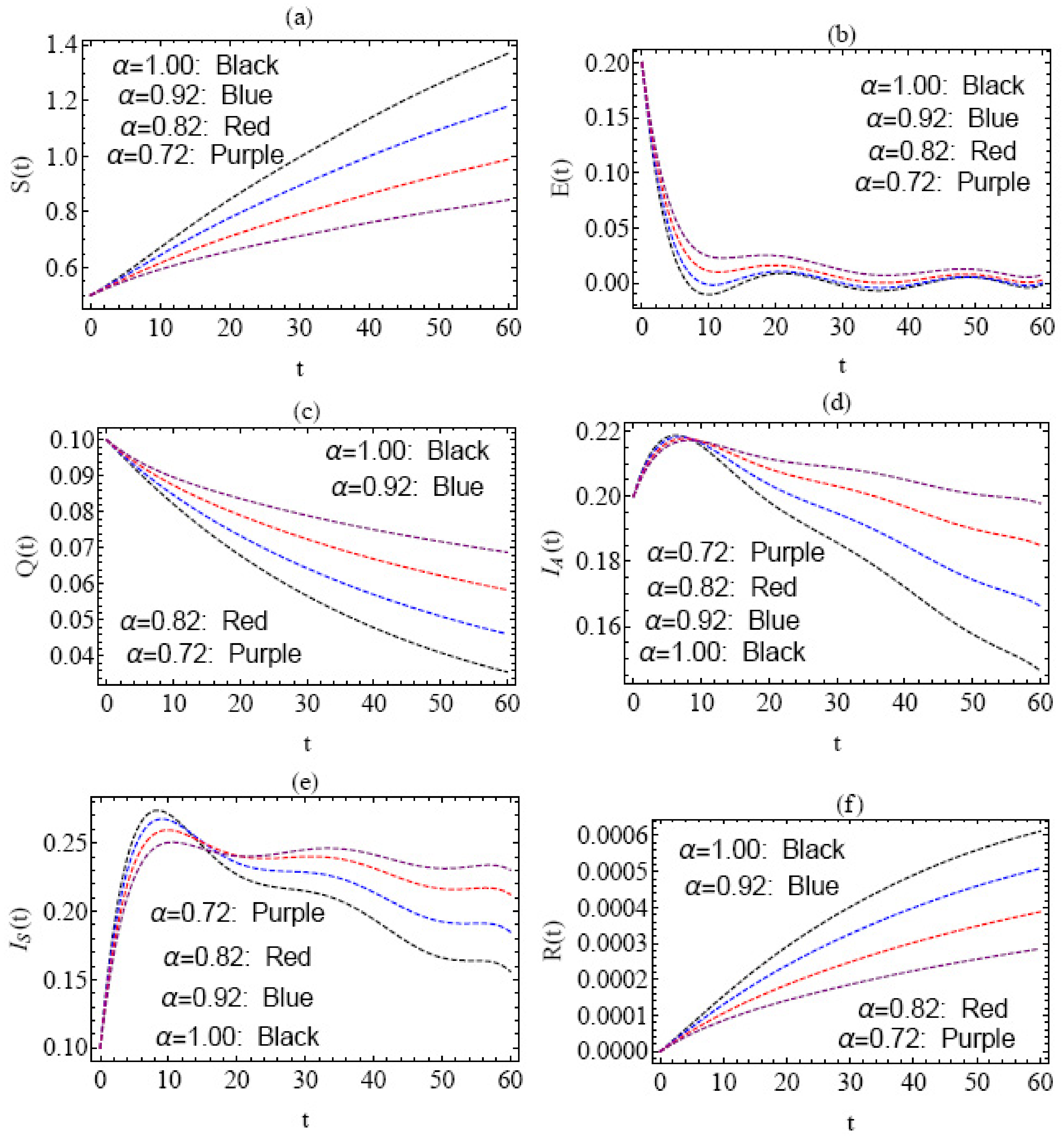
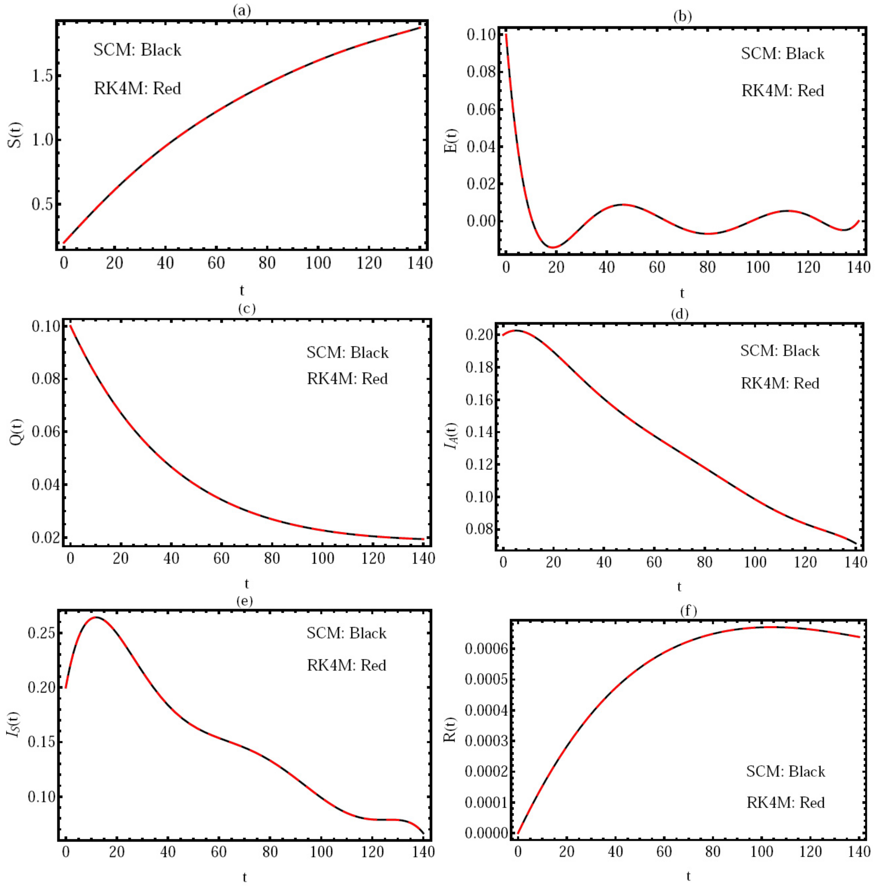
5. Numerical Simulation

We look at the proposed system in (11) with the following parameter values [31]:

$$\tau =0.0002,\beta =0.0805,\delta =0.000016728,\gamma =0.00020138,\eta =0.4478,\theta =0.0101,$$

$$\mu =0.0106,\upsilon =0.0003208,\sigma =0.0668,\Lambda =0.02537,r1=0.00005734,r2=0.00001673,$$

and different values of $S_0,E_0,Q_0,I{A}_0,I{S}_0,R_0.$ Figure 2, Figure 3, Figure 4, Figure 5 and Figure 6 show a numerical simulation of the investigated model using the proposed method. All codes were written and debugged by Mathematica 11 on a Dell Inspiron 15 (3593) Workstation (processor: 11th Gen Intel(R) Core(TM) i7-1165G7 and 2.80 GHz, 1.69 GHz, 32 GB Ram DDR3, and 1 TB storage).

Figure 2 depicts the behavior of the approximate solution for various fatality rate values $\Lambda =0.01,0.03,0.05,$ in the interval ($0,120$), with $N=7,h=0.05$, and initial conditions $S_0=0.5,E_0=0.2,Q_0=0.1,I{A}_0=0.2,I{S}_0=0.1,R_0=0.0$. In Figure 3, the solution for all components of the model via distinct values of $\alpha =1.0,0.92,0.82,0.72$ is presented in the interval ($0,60$), with $N=8,h=0.05$, and $S_0=0.5,E_0=0.2,Q_0=0.1,I{A}_0=0.2,I{S}_0=0.1,R_0=0.0$, where, in this case, ${\mathfrak{R}}_0=0.359916<1$, and in view of Theorem 3 we note that ${\xi }_0$ is locally asymptotically stable. In Figure 4, the behavior of the approximate solution in the domain ($0,120$) with $N=7,h=0.05$ is shown, where the components of solution $S\left(t\right),E\left(t\right),Q\left(t\right),IA\left(t\right),IS\left(t\right),R\left(t\right)$ are represented by different values of the initial conditions in Figure 4a–f, respectively. In this situation, we look at three scenarios:

i. 

$S_0=0.5,E_0=0.1,Q_0=0.1,I{A}_0=0.3,I{S}_0=0.3,R_0=0.0$;

ii. 

$S_0=0.3,E_0=0.2,Q_0=0.2,I{A}_0=0.1,I{S}_0=0.2,R_0=0.0$;

iii. 

$S_0=0.5,E_0=0.3,Q_0=0.3,I{A}_0=0.2,I{S}_0=0.1,R_0=0.0$.

In all of these circumstances, the fundamental reproduction number, ${\mathfrak{R}}_0<1$, is used.

The residual error function (REF) [34] is introduced in Figure 5 using the same parameters and domain as in Figure 2, at $N=8,h=0.05$, as well as the following initial conditions:

$$S_0=0.5,E_0=0.2,Q_0=0.1,I{A}_0=0.2,I{S}_0=0.1,R_0=0.0.$$

This figure demonstrates the accuracy of the theoretical stability findings found in the section above. Where, according to Theorem 3, the disease-free equilibrium point, ${\overline{\mathbf{E}}}_0$, is locally asymptotically stable in all of these circumstances (Figure 2, Figure 3, Figure 4 and Figure 5), and the fundamental reproduction number, ${\mathfrak{R}}_0<1$, is present in every instance.

We compared the solution generated by the proposed method with GRK4 [35] in Figure 6 with the same parameters and domain $(0,150)$ as in Figure 4, with $N=10,h=0.05$, and the initial conditions $S_0=0.2,E_0=0.1,Q_0=0.1,I{A}_0=0.2,I{S}_0=0.2,R_0=0.0.$ For more comparison, we estimated the CPU running times (in seconds) for the two techniques (the present method and the GRK4 method) with different values of N and h in

Table 1. The CPU running times for the present method and the GRK4 method.

$\mathit{\alpha }$	N	h	Present Method	GRK4 Method
1.0	8	0.005	25 s	24 s
		0.001	30 s	28 s
	10	0.005	28 s	26 s
		0.001	35 s	34 s
0.95	8	0.005	27 s	26 s
		0.001	32 s	30 s
	10	0.005	30 s	29 s
		0.001	37 s	35 s
0.90	8	0.005	28 s	27 s
		0.001	33 s	31 s
	10	0.005	31 s	30 s
		0.001	38 s	36 s

. From this table, we observed that our proposed method took CPU running times that were similar to the GRK4 method.

The behavior of the solution is dependent on $\Lambda$, the initial circumstances, and $\tau ,\beta ,\delta ,\gamma ,\eta ,\theta ,\mu ,$ $\upsilon ,\sigma ,$ $r_1,r_2$ are shown in Figure 2, Figure 3, Figure 4, Figure 5 and Figure 6, which demonstrates how the suggested strategy was effectively used to address the situation at hand. The expected behavior of the disease might have taken place, which would be a clear replication of the model.

The findings showed that as individuals came into contact with exposed or infected persons, their susceptibility declined at consistent rates, resulting in a bigger number of exposed individuals. The declines and increases were caused by people becoming infected after being exposed to COVID-19. Conversely, as a proportion of recovered people passed away from natural causes, fewer people were exposed, infected, or placed in quarantine. Moreover, there were fluctuations in the proportion of those quarantined to people who were exposed overall.

6. Conclusions and Remarks

We used the proposed method to simulate the COVID-19 model in this work. With the aid of the characteristics of the shifted Chebyshev polynomials, a rough formula for the Caputo fractional derivative was presented with a particular focus. The model was turned into an algebraic system of equations using the suggested method and this approximation for a formula. The system was then stated as a constrained optimization problem, and the problem was then optimized to find the unknown coefficients for the approximate solution. The presentation of the qualitative examination of the model was given particular importance. According to the results, the model had two equilibrium points: the endemic equilibrium point ${\overline{\mathbf{E}}}_1$ and the disease-free equilibrium point ${\overline{\mathbf{E}}}_0$. In addition, the equilibrium points showed that ${\overline{\mathbf{E}}}_0$ was locally and globally asymptotically stable depending on ${\mathfrak{R}}_0<1$, the fundamental reproduction number, whereas ${\overline{\mathbf{E}}}_1$ depended on ${\mathfrak{R}}_0>1$. The profile of each state variable and the fitted values of the parameters were used to illustrate the spread of the disease. The parameters in ${\mathfrak{R}}_0$ were also subjected to a sensitivity analysis. The contact rate between susceptible individuals and the transfer rate of people from exposure to symptomatically infected classes made up the most sensitive ${\mathfrak{R}}_0$ criteria.

The solutions obtained with various values for the parameters, as well as the initial conditions for the studied problem, demonstrated that the offered method is well suited to successfully explore this model. In addition, the REF was calculated to ensure that the suggested technique is genuine. The outcomes confirmed that the suggested methodology is a useful tool for examining the numerical solution for such models. By incorporating this numerical analysis, our study, on the other hand, may offer more solid physical interpretations for previous theoretical and computational studies on this subject. We intend to deal with this model in the future, but on a larger scale, by generalizing this research to include additional types of polynomials or fractional derivatives. The Mathematica software program was used to perform numerical simulation operations.

References

1. Anderson, R.M.; May, R.M. Helminth infections of humans: Mathematical models, population dynamics, and control. Adv. Parasitol. 1985, 24, 1–101. [Google Scholar]
2. Edelstein, K.L. Mathematical Models in Biology; SIAM: Philadelphia, PA, USA, 2005. [Google Scholar]
3. Khader, M.M.; Sweilam, N.H.; Mahdy, A.M.S.; Moniem, N.K.A. Numerical simulation for the fractional SIRC model and influenxa A. Appl. Math. Inf. Sci. 2014, 8, 1029–1036. [Google Scholar] [CrossRef]
4. World Health Organization. Novel Coronavirus Diseases 2019. Available online: https://www.who.int/emergencies/diseases/novel-coronavirus-2019 (accessed on 14 October 2020).
5. Ajisegiri, W.; Odusanya, O.; Joshi, R. COVID-19 outbreak situation in Nigeria and the need for effective engagement of community health workers for epidemic response. Glob. Biosecur. 2020, 1, 5–20. [Google Scholar] [CrossRef]
6. Ahmad, S.; Ullah, A.; Al-Mdallal, Q.M.; Khan, H.; Shah, K.; Khan, A. Fractional order mathematical modeling of COVID-19 transmission. Chaos Solitons Fractals 2020, 139, 110256. [Google Scholar] [CrossRef]
7. Baud, D.; Qi, X.; Nielsen-Saine, K.; Musso, D.; Pomar, L.; Favre, G. Real estimates of mortality following covid-19 infection. Lancet Infect. Dis. 2020, 11, 13–23. [Google Scholar] [CrossRef] [Green Version]
8. Koo, J.R.; Cook, A.R.; Park, M.; Sun, Y.; Sun, H.; Lim, J.T.; Tam, C.; Dickens, B.L. Interventions to mitigate early spread of sarscov-2 in singapore: A modelling study. Lancet Infect. Dis. 2020, 15, 15–25. [Google Scholar]
9. Adegboye, O.A.; Adekunle, A.I.; Gayawan, E. Early transmission dynamics of novel coronavirus (covid-19) in Nigeria. Int. J. Environ. Res. Public Health 2020, 17, 10–25. [Google Scholar] [CrossRef] [PubMed]
10. Cao, Y.; Nikan, O.; Avazzadeh, Z. A localized meshless technique for solving 2D nonlinear integro-differential equation with multi-term kernels. Appl. Numer. Math. 2023, 183, 140–156. [Google Scholar] [CrossRef]
11. Kalimbetov, B.; Abylkasymova, E.; Beissenova, G. On the asymptotic solutions of singulary perturbed differential systems of fractional order. J. Math. Comput. Sci. 2022, 24, 165–172. [Google Scholar] [CrossRef]
12. Asjad, M.I.; Ullah, N.; Rehman, H.U.; Baleanu, D. Optical solitons for conformable space-time fractional nonlinear model. J. Math. Comput. Sci. 2022, 27, 28–41. [Google Scholar] [CrossRef]
13. Xie, J.; Yan, X.; Ali, M.A.; Hammouch, Z. A linear decoupled physical-property-preserving difference method for fractional-order generalized Zakharov system. J. Comput. Appl. Math. 2023, 426, 115044. [Google Scholar] [CrossRef]
14. Danane, J.; Allali, K.; Hammouch, Z. Mathematical analysis of a fractional differential model of HBV infection with antibody immune response. Chaos Solitons Fractals 2020, 136, 109787. [Google Scholar] [CrossRef]
15. Hajji, M.A.; Al-Mdallal, Q. Numerical simulations of a delay model for immune system-tumor interaction. Sultan Qaboos Univ. J. Sci. 2018, 23, 19–31. [Google Scholar] [CrossRef] [Green Version]
16. Abd-Elhameed, W.M. New Galerkin operational matrix of derivatives for solving Lane-Emden singular-type equations. Eur. Phys. J. Plus 2015, 130, 52. [Google Scholar] [CrossRef]
17. Khader, M.M.; Adel, M. Modeling and numerical simulation for covering the fractional COVID-19 model using spectral collocation-optimization algorithms. Fractal Fract. 2022, 6, 363. [Google Scholar] [CrossRef]
18. Sweilam, N.H.; Khader, M.M.; Adel, M. On the fundamental equations for modeling neuronal dynamics. J. Adv. Res. 2014, 5, 253–259. [Google Scholar] [CrossRef] [Green Version]
19. Adel, M.; Srivastava, H.M.; Khader, M.M. Implementation of an accurate method for the analysis and simulation of electrical R-L circuits. Math. Methods Appl. Sci. 2022, 12, 8062. [Google Scholar] [CrossRef]
20. Kolwankar, K.M.; Gangal, A.D. Fractional differentiability of nowhere differentiable functions and dimensions. Chaos Interdiscip. J. Nonlinear Sci. 1996, 6, 505–513. [Google Scholar] [CrossRef] [Green Version]
21. Atta, A.G.; Youssri, Y.H. Advanced shifted first-kind Chebyshev collocation approach for solving the nonlinear time-fractional partial integro-differential equation with a weakly singular kernel. Comput. Appl. Math. 2022, 6, 381. [Google Scholar] [CrossRef]
22. Abd-Elhameed, W.M. Novel expressions for the derivatives of sixth kind chebyshev polynomials: Spectral solution of the non-linear one-dimensional burgers’ equation. Fractal Fract. 2021, 5, 53. [Google Scholar] [CrossRef]
23. Youssri, Y.H.; Atta, A.G. Spectral collocation approach via normalized shifted Jacobi polynomials for the nonlinear Lane-Emden equation with fractal-fractional derivative. Fractal Fract. 2023, 7, 133. [Google Scholar] [CrossRef]
24. Khader, M.M.; Saad, K.M. A numerical study using Chebyshev collocation method for a problem of biological invasion: Fractional Fisher equation. Int. J. Biomath. 2018, 11, 1850099. [Google Scholar] [CrossRef]
25. Atta, A.G.; Abd-Elhameed, W.M.; Moatimid, G.M.; Youssri, Y.H. Shifted fifth-kind Chebyshev Galerkin treatment for linear hyperbolic first-order partial differential equations. Appl. Numer. Math. 2021, 167, 237–256. [Google Scholar] [CrossRef]
26. Saad, K.M.; Khader, M.M.; Gomez-Aguilar, J.F.; Baleanu, D. Numerical solutions of the fractional Fisher’s type equations with Atangana-Baleanu fractional derivative by using spectral collocation methods. Chaos 2019, 29, 023116. [Google Scholar] [CrossRef] [PubMed]
27. Kumar, S.; Gomez-Aguilar, J.F.; Lavin-Delgado, J.E.; Baleanu, D. Derivation of operational matrix of Rabotnov fractional-exponential kernel and its application to fractional Lienard equation. Alex. Eng. J. 2020, 59, 991–2997. [Google Scholar] [CrossRef]
28. Snyder, M.A. Chebyshev Methods in Numerical Approximation; Prentice-Hall, Inc.: Englewood Cliffs, NJ, USA, 1966. [Google Scholar]
29. Mason, J.C.; Handscomb, D.C. Chebyshev Polynomials; Chapman and Hall: New York, NY, USA; CRC: Boca Raton, FL, USA, 2003. [Google Scholar]
30. Handan, C.Y. Numerical solution of fractional Riccati differential equation via shifted Chebyshev polynomials of the third kind. J. Eng. Technol. Appl. Sci. 2017, 28, 1–11. [Google Scholar]
31. Ahmed, I.; Modu, G.U.; Yusuf, A.; Kumam, P.; Yusuf, I. A mathematical model of coronavirus disease (COVID-19) containing asymptomatic and symptomatic classes. Results Phys. 2021, 21, 103776. [Google Scholar] [CrossRef]
32. Diekmann, O.; Heesterbeek, J.A.P.; Metz, J.A. On the definition and the computation of the basic reproduction ratio R0 in models for infectious diseases in heterogeneous populations. J. Math. Biol. 1990, 28, 365–382. [Google Scholar] [CrossRef] [Green Version]
33. El-Hawary, H.M.; Salim, M.S.; Hussien, H.S. Ultraspherical integral method for optimal control problems governed by ordinary differential equations. J. Glob. Optim. 2003, 25, 283–303. [Google Scholar] [CrossRef]
34. Parand, K.; Delkhosh, M. Operational matrices to solve nonlinear Volterra-Fredholm integro-differential equations of multi-arbitrary order. Gazi Univ. J. Sci. 2016, 29, 895–907. [Google Scholar]
35. Ibrahim, Y.F.; Khader, M.M.; Megahed, A.; Abd Elsalam, F.; Adel, M. An efficient numerical simulation for the fractional COVID-19 model by using the GRK4M together and the fractional FDM. Fractal Fract. 2022, 6, 304. [Google Scholar] [CrossRef]
Figure 1. Flowchart describing the dynamics of spread in the model for COVID-19.
Fractalfract 07 00307 g001
Figure 2. Behavior of the approximate solution via different values of Λ . (af) S ( t ) , E ( t ) , Q ( t ) , I A ( t ) , I S ( t ) , R ( t ) .
Fractalfract 07 00307 g002
Figure 3. Behavior of the approximate solution via different values of α . (af) S ( t ) , E ( t ) , Q ( t ) , I A ( t ) , I S ( t ) , R ( t ) .
Fractalfract 07 00307 g003
Figure 4. Behavior of the approximate solution via different values of initial values. (af) S ( t ) , E ( t ) , Q ( t ) , I A ( t ) , I S ( t ) , R ( t ) .
Fractalfract 07 00307 g004
Figure 5. The REF of the approximate solution. (af) S ( t ) , E ( t ) , Q ( t ) , I A ( t ) , I S ( t ) , R ( t ) .
Fractalfract 07 00307 g005
Figure 6. Comparison the solution obtained by the proposed method and the GRK4M method. (af) S ( t ) , E ( t ) , Q ( t ) , I A ( t ) , I S ( t ) , R ( t ) .
Fractalfract 07 00307 g006