Sub-Diffusion Two-Temperature Model and Accurate Numerical Scheme for Heat Conduction Induced by Ultrashort-Pulsed Laser Heating

Abstract

In this study, we propose a new sub-diffusion two-temperature model and its accurate numerical method by introducing the Knudsen number ($K_n$) and two Caputo fractional derivatives ($0<\alpha ,\beta <1$) in time into the parabolic two-temperature model of the diffusive type. We prove that the obtained sub-diffusion two-temperature model is well posed. The numerical scheme is obtained based on the $L1$ approximation for the Caputo fractional derivatives and the second-order finite difference for the spatial derivatives. Using the discrete energy method, we prove the numerical scheme to be unconditionally stable and convergent with $O({\tau }^{min\{2-\alpha ,2-\beta \}}+h^2)$, where $\tau ,h$ are time and space steps, respectively. The accuracy and applicability of the present numerical scheme are tested in two examples. Results show that the numerical solutions are accurate, and the present model and its numerical scheme could be used as a tool by changing the values of the Knudsen number and fractional-order derivatives as well as the parameter in the boundary condition for analyzing the heat conduction in porous media, such as porous thin metal films exposed to ultrashort-pulsed lasers, where the energy transports in phonons and electrons may be ultraslow at different rates.

1. Introduction

Ultrashort-pulsed laser heating technology has been widely used in thermal processing of materials, such as the structural monitoring of thin metal films, laser micro-machining, laser patterning, structural tailoring of microfilms, and laser processing in thin-film deposition [1]. The advantages of using lasers over the conventional manufacturing method are well addressed in [2]. In particular, ultrashort-pulsed lasers with pulse durations of the order of sub-picoseconds to femtoseconds possess exclusive capabilities in limiting the undesirable spread of the thermal process zone in the heated sample [3]. A better understanding of energy transfer in the thermal processing of materials by ultrafast laser heating is critical in many applications, such as the decrease in excessive heating and thermal damage to the gold-coated metal mirrors of high-power infrared-laser systems [4], effective thermal management of next-generation electron and optoelectronic devices [5].

For an ultrashort-pulsed laser, the heating involves high-rate heat flow from electrons to lattices in picosecond domains. When a metal is heated by lasers, the photon energy is primarily absorbed by the free electrons that are confined within skin depth during the excitation. Electron temperatures first shoot up to several hundreds or thousands of degrees within a few of picoseconds without significantly disturbing the metal lattices. A major portion of the thermal electron energy is then transferred to the lattices; meanwhile, another part of the energy diffuses to the electrons in the deeper region of the target. Because the pulse duration is so short, the laser is turned off before thermal equilibrium between electrons and lattices is reached. This stage is often called the non-equilibrium heating due to the large difference of temperatures between the electrons and the lattices [6,7].

Following earlier models by Kagnaov et al. [8] and Anisimov et al. [9], Qiu and Tien [4,10,11] proposed a parabolic two-step (two-temperature) energy transport method (PTTM) based on the phonon–electron interaction to analyze heat conduction in microscale metals when energy is induced by ultrashort-pulsed laser heating. The model is expressed as follows:

$$\begin{array}{c}{C}_e\frac{\partial T_e}{\partial t}(x,t)=k_e\frac{{\partial }^2{T}_e(x,t)}{\partial x^2}-G[T_e(x,t)-T_l(x,t)]+Q(x,t),\hfill \end{array}$$

(1)

$$\begin{array}{c}{C}_l\frac{\partial T_l}{\partial t}(x,t)=G[T_e(x,t)-T_l(x,t)],\hfill \end{array}$$

(2)

where $T_e$ is the electron temperature, $T_l$ is the lattice temperature, $k_e$ is the conductivity, $C_e$ and $C_l$ are the electron heat capacity and the lattice heat capacity, respectively, G is the electron–lattice coupling factor, and $Q(x,t)$ is the energy absorption rate given by [7]

$$Q(x,t)=Q_{0}exp[-\frac{x}{\delta }]I\left(t\right).$$

(3)

Here, $Q_0$ is the intensity of the laser absorption rate, $\delta$ is the optical penetration depth, and $I\left(t\right)$ is the light intensity of the laser beam. It should be pointed out that the laser absorption rate is an important parameter, which needs to be carefully calculated [12]. Qiu and Tien [4,10,11] obtained an experimentally fitted expression of $Q(x,t)$ for thin gold films as

$$Q(x,t)=0.94J\frac{1-R}{t_p\delta }exp\left[-\frac{x}{\delta }-2.77{\left(\frac{t-2t_p}{t_p}\right)}^2\right],$$

(4)

where J is the laser fluence, R is the surface reflectivity, and $t_p$ is the laser pulse duration in femtosecond.

The fractional calculus has been successfully used to modulate several models in heat conduction and other media and has gained much importance in the heat conduction and thermoelastic problems [13]. Sherief et al. [14] suggested the fractional non-Fourier law as $q(r,t)+\tau D_t^{\alpha }q(r,t)=k\nabla T(r,t)$, $0<\alpha \le 1$, where $D_t^{\alpha }$ is the Caputo time-fractional derivative. Youssef [15] assumed another form for the non-Fourier law as $q(r,t)+\tau \partial q(r,t)/\partial t=k{I}_{\alpha }\nabla T(r,t)$, $0<\alpha \le 2$, where $I_{\alpha }$ is the conventional Riemann–Louiville fractional integral. A fractional-order generalized DPL model was applied for nanoscale head transfer in electro-magneto-thermoelastic media [16,17]. More recently, we, with Sun [18,19], proposed numerical methods for solving the time-fractional dual-phase-lagging heat conduction equation with the temperature-jump boundary condition. We [20] further presented a numerical algorithm to speed up the computation for solving the time-fractional dual-phase-lagging nanoscale heat conduction equation. Shen and Dai with their collaborators [21,22] presented a fractional parabolic two-step model and fractional diffusion-wave two-step model and numerical schemes for nanoscale heat conduction, where the fractional derivatives in electron and phonon equations are in the same order. Mozafarifard et al. [23] proposed a two-temperature time-fractional model for electron–phonon coupled interfacial thermal transport, where the fractional derivative appears only in the electron equation, while the phonon equation is a common diffusion equation.

The heat conduction in porous media, such as porous thin metal films exposed to ultrashort-pulsed lasers, could be different from that in non-porous thin metal films exposed to ultrashort-pulsed lasers because of the porosity. As pointed out in [24], the model with the Caputo fractional derivative ($0<\alpha <1$) in time governs the ultraslow diffusion, which is called the sub-diffusion model and is often used to govern the heat conduction in porous materials. Thus, the purpose of this study is to propose a sub-diffusion two-temperature model and its accurate numerical method by introducing the Knudsen number ($K_n$) and two Caputo fractional derivatives ($0<\alpha ,\beta <1$) in time into the parabolic two-temperature (electron and phonon) model of the diffusive type (i.e., both electron and phonon energy transport equations are diffusion equations, which is different from the original two-temperature model). By changing values of the Knudsen number and fractional-order derivatives as well as the parameter in the boundary condition, the simulation could be a tool for analyzing the heat conduction in porous media such as porous thin metal films exposed to ultrashort-pulsed lasers, where the energy transports in phonon and free electron may be ultraslow at different rates. To this end, we first introduce two Caputo fractional derivatives ($0<\alpha ,\beta <1$) in time into the parabolic two-temperature model of the diffusive type (which we may call the sub-diffusion two-temperature (SD-TT) model) as follows:

$$\begin{array}{c}{C}_e{t}_f^{\alpha -1}·{}_0^C{D}_t^{\alpha }{T}_e(x,t)=k_e\frac{{\partial }^2{T}_e(x,t)}{\partial x^2}-G[T_e(x,t)-T_l(x,t)]+S(x,t),\hfill \end{array}$$

(5)

$$\begin{array}{c}{C}_l{t}_f^{\beta -1}·{}_0^C{D}_t^{\beta }{T}_l(x,t)=k_l\frac{{\partial }^2{T}_l(x,t)}{\partial x^2}+G[T_e(x,t)-T_l(x,t)],\hfill \end{array}$$

(6)

within the domain of $0\le x\le L_c$, $0\le t\le t_F$ and $0<\alpha ,\beta <1$, where $t_f$ is the phonon mean free time, C is the volumetric heat capacity, k is the thermal conductivity, and $S(x,t)$ is the energy absorption rate. The subscripts e and l represent the electron and lattice, respectively. ${}_0^C{D}_t^{\alpha }{T}_e(x,t)$ and ${}_0^C{D}_t^{\beta }{T}_l(x,t)$ are the Caputo fractional derivatives defined by [24]

$$\begin{array}{c}{}_0^C{D}_t^{\alpha }{T}_e(x,t)=\frac{1}{\mathsf{\Gamma }(1-\alpha )}{\int }_0^t\frac{\partial T_e(x,s)}{\partial s}\frac{ds}{{(t-s)}^{\alpha }},0<\alpha <1;\hfill \end{array}$$

(7)

$$\begin{array}{c}{}_0^C{D}_t^{\beta }{T}_l(x,t)=\frac{1}{\mathsf{\Gamma }(1-\beta )}{\int }_0^t\frac{\partial T_l(x,s)}{\partial s}\frac{ds}{{(t-s)}^{\beta }},0<\beta <1.\hfill \end{array}$$

(8)

In addition, in order to catch the effects of boundary phonon scattering inside a nano-size geometry, the temperature-jump boundary condition (a Robin boundary condition), $T-T_w=\gamma K_n{\left(\frac{\partial T}{\partial \overline{n}}\right)}_w$ was introduced to couple with the fractional two-step (FTS) model (5) and (6). Here, $T_w$ is the wall temperature, $K_n$ is the Knudsen number, and $\gamma$ should be determined in such a way that the results of the heat conduction model coincide with the solution of the BTE [25].

The SD-TT model (5) and (6) denotes a fractional form of the diffusive two-temperature model. When $\alpha =\beta =1$, the SD-TT model (5) and (6) reduces to the diffusive two-temperature model, while when $\beta =1$, the SD-TT model (5) and (6) reduces to the two-temperature time-fractional model given in [23]. The purpose of two different Caputo factional derivatives $(0<\alpha ,\beta <1)$ is to deal with the case where the energy transports in the phonon and electron may be ultraslow at different rates. Since the present SD-TT model with initial and boundary conditions is difficult to solve analytically in general, in this study, we present an accurate finite difference scheme for solving the SD-TT model (5) and (6) with initial and temperature-jump boundary conditions.

The rest of the article is organized as follows: In Section 2, we introduce non-dimensional parameters to transform the SD-TT model in dimensionless. We then derive an energy estimate for ensuring the model to be well posed. In Section 3, we construct an accurate difference scheme for solving the mathematical model. In Section 4, the unconditional stability and convergence of the scheme are rigorously analyzed. In Section 5, we test a numerical example to verify the theoretical analysis and give another example showing the applicability of the model. Finally, we summarize the main results of this study in Section 6.

2. Sub-Diffusion Two-Temperature Model

We introduce non-dimensional parameters as follows:

$$\left\{\begin{array}{c}{x}^{★}=\frac{x}{L_c},x_s^{★}=\frac{x_s}{L_c},t^{★}=\frac{t}{t_f},t_p^{★}=\frac{t_p}{t_f},\hfill \\ K_n=\frac{l_f}{L_c},B=\frac{C_l}{C_e},G^{★}=\frac{t_{f}G}{C_e},\hfill \\ T_e^{★}=\frac{T_e-T_0}{T_0},T_l^{★}=\frac{T_l-T_0}{T_0},T_w^{★}=\frac{T_w-T_0}{T_0},\hfill \end{array}\right.$$

(9)

together with $k=\frac{1}{3}C\left|v\right|l_f$, $\left|v\right|=l_f/t_f$, where $T_0$ is the reference temperature, and v is the heat carrier group velocity. Substituting Equation (9) into Equations (5) and (6) and using the fact that

$$\left.\begin{array}{c}\hfill \frac{k_e{t}_f}{L_c^2{C}_e}=\frac{C_e\left|v\right|l_f{t}_f}{3L_c^2{C}_e}\\ \hfill \frac{k_l{t}_f}{L_c^2{C}_l}=\frac{C_l\left|v\right|l_f{t}_f}{3L_c^2{C}_l}\end{array}\right\}=\frac{1}{3}{\left(\frac{l_f}{L_c}\right)}^2=\frac{1}{3}{K}_n^2,$$

(10)

we obtain the sub-diffusion two-temperature (SD-TT) dimensionless energy transport equation as follows:

$$\begin{array}{c}{}_0^C{D}_{t^{★}}^{\alpha }{T}_e^{★}=\frac{K_n^2}{3}\frac{{\partial }^2{T}_e^{★}}{\partial {x^{★}}^2}-G^{★}(T_e^{★}-T_l^{★})+S^{★}(x^{★},t^{★}),\hfill \end{array}$$

(11)

$$\begin{array}{c}B{}_0^C{D}_{t^{★}}^{\beta }{T}_l^{★}=\frac{B{K}_n^2}{3}\frac{{\partial }^2{T}_l^{★}}{\partial {x^{★}}^2}+G^{★}(T_e^{★}-T_l^{★}),x^{★}\in (0,1),t^{★}\in (0,t_F/t_f],\hfill \end{array}$$

(12)

subject to the initial condition

$$T_e^{★}(x^{★},0)=T_1\left(x^{★}\right),T_l^{★}(x^{★},0)=T_2\left(x^{★}\right),x^{★}\in [0,1]$$

(13)

and the Robin boundary conditions ( i.e., the temperature-jump condition)

$$\begin{array}{c}\left[-\gamma K_n\frac{\partial T_e^{★}}{\partial x^{★}}+T_e^{★}\right]{|}_{x^{★}=0}=T_w^e(0,t^{★}),\left[\gamma K_n\frac{\partial T_e^{★}}{\partial x^{★}}+T_e^{★}\right]{|}_{x^{★}=1}=T_w^e(1,t^{★}),t^{★}\in (0,t_F/t_f],\hfill \end{array}$$

(14)

$$\begin{array}{c}\left[-\gamma K_n\frac{\partial T_l^{★}}{\partial x^{★}}+T_l^{★}\right]{|}_{x^{★}=0}=T_w^l(0,t^{★}),\left[\gamma K_n\frac{\partial T_l^{★}}{\partial x^{★}}+T_l^{★}\right]{|}_{x^{★}=1}=T_w^l(1,t^{★}),t^{★}\in (0,t_F/t_f].\hfill \end{array}$$

(15)

We now analyze the well posedness of the SD-TT model (11)–(15). To this end, we first present a useful lemma, which will be used for obtaining an energy estimation of the governing model (11)–(15). For simplicity, we omit asterisk in Equations (11)–(15) during the derivations of the well-posedness and the finite difference scheme and the corresponding theoretical analysis in the next two sections.

Lemma 1.

For any $w\left(x\right)\in C^1[0,L]$, it holds that

$${\int }_0^L{w}^2\left(x\right)dx\le \frac{L}{2}(1+ϵ)[w^2\left(0\right)+w^2\left(L\right)]+\frac{L^2}{6}\left(1+\frac{1}{ϵ}\right){\int }_0^L{\left(w^{\prime }\left(x\right)\right)}^{2}dx,$$

where ϵ is a positive constant.

Proof of Lemma 1.

According to Lemma 2.2 in [18], for any $x\in (0,L)$, we have

$$L{w}^2\left(x\right)\le (1+ϵ)[(L-x)w^2\left(0\right)+x{w}^2\left(L\right)]+\left(1+\frac{1}{ϵ}\right)x(L-x){\int }_0^L{\left(w^{\prime }\left(s\right)\right)}^{2}ds.$$

(16)

Integrating Equation (16) with respect to x from 0 to L yields

$$\begin{array}{cc}\hfill L{\int }_0^L{w}^2\left(x\right)dx\le & (1+ϵ)\left[w^2\left(0\right)·{\int }_0^L(L-x)dx+w^2\left(L\right)·{\int }_0^{L}xdx\right]\hfill \\ & +\left(1+\frac{1}{ϵ}\right){\int }_0^L{\left(w^{\prime }\left(s\right)\right)}^{2}ds·{\int }_0^{L}x(L-x)dx\hfill \\ \hfill =& \frac{L^2}{2}(1+ϵ)[w^2\left(0\right)+w^2\left(L\right)]+\frac{L^3}{6}\left(1+\frac{1}{ϵ}\right){\int }_0^L{\left(w^{\prime }\left(s\right)\right)}^{2}ds.\hfill \end{array}$$

(17)

Dividing Equation (17) by L, we arrive at the conclusion.  □

Theorem 1.

Let $\{T_e,T_l\}$ be the solution of the SD-TT model (11)–(15), subject to the homogeneous boundary conditions. Then, it holds that

$${\int }_0^1{T}_l^2(x,t)dx\le \left(\frac{1}{G}+\frac{6c}{K_n^2}\right)F\left(t\right)+{\int }_0^t\left(\frac{1}{G}+\frac{6c}{K_n^2}{e}^{t-s}\right)F\left(s\right)ds+\frac{1}{G}{\int }_0^t{\int }_0^{s}F\left(\eta \right)e^{s-\eta }d\eta ds;$$

(18)

$${\int }_0^1{T}_e^2(x,t)dx\le \frac{3c}{K_n^2}F\left(t\right)+\frac{3c}{K_n^2}{\int }_0^{t}F\left(s\right)e^{t-s}ds;$$

(19)

and

$$\underset{0\le x\le 1}{max}{\left|T_l(x,t)\right|}^2\le \frac{3(1+4\gamma K_n)}{8B{K}_n^2}\left[F\left(t\right)+{\int }_0^{t}F\left(s\right)ds+{\int }_0^t{\int }_0^{s}F\left(\eta \right)e^{s-\eta }d\eta ds\right];$$

(20)

$$\underset{0\le x\le 1}{max}{\left|T_e(x,t)\right|}^2\le \frac{3}{4}\frac{1+4\gamma K_n}{K_n^2}\left[F\left(t\right)+{\int }_0^{t}F\left(s\right)e^{t-s}ds\right],$$

(21)

with $c=\frac{1+3\gamma K_n}{6}$, where $F\left(t\right)$ is defined by

$$\begin{array}{c}F\left(t\right)=2E_1\left(0\right)+2E_2\left(0\right)+2G{\int }_0^1{[T_e(x,0)-T_l(x,0)]}^{2}dx+\frac{K_n^2}{3c}{\int }_0^1{T}_e^2(x,0)dx\hfill \\ +\frac{12c}{K_n^2}\left[{\int }_0^1{S}^2(x,0)dx+{\int }_0^1{S}^2(x,t)dx+{\int }_0^t{\int }_0^1{\left(\frac{\partial S}{\partial \eta }(x,\eta )\right)}^{2}dxd\eta \right]\hfill \end{array}$$

(22)

and

$$\begin{array}{c}{E}_1\left(t\right)=\frac{K_n^2}{3}\left[{\int }_0^1{\left(\frac{\partial T_e}{\partial x}\right)}^{2}dx+\frac{1}{\gamma K_n}\left(T_e^2(0,t)+T_e^2(1,t)\right)\right],\hfill \end{array}$$

(23)

$$\begin{array}{c}{E}_2\left(t\right)=\frac{B{K}_n^2}{3}\left[{\int }_0^1{\left(\frac{\partial T_l}{\partial x}\right)}^{2}dx+\frac{1}{\gamma K_n}\left(T_l^2(0,t)+T_l^2(1,t)\right)\right].\hfill \end{array}$$

(24)

Proof of Theorem 1.

We multiply Equation (11) by $\frac{\partial T_e}{\partial t}$ and Equation (12) by $\frac{\partial T_l}{\partial t}$, respectively, and integrate the results with respect to x from 0 to 1. This gives

$${\int }_0^1\frac{\partial T_e}{\partial t}·{}_0^C{D}_t^{\alpha }{T}_{e}dx=\frac{K_n^2}{3}{\int }_0^1\frac{\partial T_e}{\partial t}·\frac{{\partial }^2{T}_e}{\partial x^2}dx-G{\int }_0^1\frac{\partial T_e}{\partial t}·(T_e-T_l)dx+{\int }_0^1\frac{\partial T_e}{\partial t}·Sdx;$$

(25)

$$B{\int }_0^1\frac{\partial T_l}{\partial t}·{}_0^C{D}_t^{\beta }{T}_{l}dx=\frac{B{K}_n^2}{3}{\int }_0^1\frac{\partial T_l}{\partial t}·\frac{{\partial }^2{T}_l}{\partial x^2}dx+G{\int }_0^1\frac{\partial T_l}{\partial t}·(T_e-T_l)dx.$$

(26)

We now estimate each term in Equations (25) and (26) as follows. We use Lemma 1 in [19] for the terms on the left-hand side of Equations (25) and (26) to obtain

$${\int }_0^1\frac{\partial T_e}{\partial t}·{}_0^C{D}_t^{\alpha }{T}_{e}dx\ge \frac{1}{2}\frac{d}{dt}{\int }_0^1{}_0^R{D}_t^{-\alpha }{\left({}_0^C{D}_t^{\alpha }{T}_e\right)}^{2}dx;$$

(27)

$$B{\int }_0^1\frac{\partial T_l}{\partial t}·{}_0^C{D}_t^{\beta }{T}_{l}dx\ge \frac{B}{2}\frac{d}{dt}{\int }_0^1{}_0^R{D}_t^{-\beta }{\left({}_0^C{D}_t^{\beta }{T}_l\right)}^{2}dx,$$

(28)

where ${}_0^R{D}_t^{-\alpha }$ and ${}_0^R{D}_t^{-\beta }$ denote the Riemann–Liouville fractional integral [24] of order $\alpha$ and $\beta$, respectively. For the first terms on the right-hand side of Equations (25) and (26), we use the integration by parts and the homogeneous boundary conditions to obtain

$$\frac{K_n^2}{3}{\int }_0^1\frac{\partial T_e}{\partial t}·\frac{{\partial }^2{T}_e}{\partial x^2}dx=-\frac{1}{2}\frac{d}{dt}{E}_1\left(t\right),$$

(29)

and

$$\frac{B{K}_n^2}{3}{\int }_0^1\frac{\partial T_l}{\partial t}·\frac{{\partial }^2{T}_l}{\partial x^2}dx=-\frac{1}{2}\frac{d}{dt}{E}_2\left(t\right).$$

(30)

We then rewrite the last term on the right-hand side of Equation (25) as

$${\int }_0^1\frac{\partial T_e}{\partial t}·Sdx=\frac{d}{dt}{\int }_0^1{T}_e·Sdx-{\int }_0^1{T}_e·\frac{\partial S}{\partial t}dx.$$

(31)

Inserting Equations (27), (29), (31) into Equation (25) and Equations (28), (30) into Equation (26), respectively, and adding the results, and noticing the following result

$$-G{\int }_0^1\frac{\partial T_e}{\partial t}·(T_e-T_l)dx+G{\int }_0^1\frac{\partial T_l}{\partial t}·(T_e-T_l)dx=-\frac{G}{2}\frac{d}{dt}{\int }_0^1{[T_e-T_l]}^{2}dx,$$

we have

$$\begin{array}{cc}\hfill \frac{1}{2}& \frac{d}{dt}\left[E_1\left(t\right)+E_2\left(t\right)+G{\int }_0^1{[T_e-T_l]}^{2}dx+{\int }_0^1{}_0^R{D}_t^{-\alpha }{\left({}_0^C{D}_t^{\alpha }{T}_e\right)}^{2}dx+B{\int }_0^1{}_0^R{D}_t^{-\beta }{\left({}_0^C{D}_t^{\beta }{T}_l\right)}^{2}dx\right]\hfill \\ & \le \frac{d}{dt}{\int }_0^1{T}_e·Sdx-{\int }_0^1{T}_e·\frac{\partial S}{\partial t}dx.\hfill \end{array}$$

(32)

We integrate Equation (32) with respect to t and notice the nonnegativity of the last two terms in square brackets. This gives

$$\begin{array}{cc}\hfill & E_1\left(t\right)+E_2\left(t\right)+G{\int }_0^1{[T_e(x,t)-T_l(x,t)]}^{2}dx\hfill \\ \hfill \le & E_1\left(0\right)+E_2\left(0\right)+G{\int }_0^1{[T_e(x,0)-T_l(x,0)]}^{2}dx-2{\int }_0^1{T}_e(x,0)·S(x,0)dx\hfill \\ \hfill & +2{\int }_0^1{T}_e(x,t)·S(x,t)dx-2{\int }_0^t{\int }_0^1{T}_e(x,\eta )·\frac{\partial S}{\partial \eta }(x,\eta )dxd\eta .\hfill \end{array}$$

(33)

Using the Cauchy–Schwarz inequality for the last three terms on the right-hand-side of Equation (33), we obtain

$$-2{\int }_0^1{T}_e(x,0)·S(x,0)dx\le \frac{K_n^2}{6c}{\int }_0^1{T}_e^2(x,0)dx+\frac{6c}{K_n^2}{\int }_0^1{S}^2(x,0)dx;$$

(34)

and

$$\begin{array}{cc}\hfill 2{\int }_0^1{T}_e(x,t)·S(x,t)dx\le & \frac{K_n^2}{6c}{\int }_0^1{T}_e^2(x,t)dx+\frac{6c}{K_n^2}{\int }_0^1{S}^2(x,t)dx;\hfill \end{array}$$

(35)

$$\begin{array}{cc}\hfill -2{\int }_0^t{\int }_0^1{T}_e(x,\eta )·\frac{\partial S}{\partial \eta }(x,\eta )dxd\eta \le & \frac{K_n^2}{6c}{\int }_0^t{\int }_0^1{T}_e^2(x,\eta )dxd\eta +\frac{6c}{K_n^2}{\int }_0^t{\int }_0^1{\left(\frac{\partial S}{\partial \eta }(x,\eta )\right)}^{2}dxd\eta .\hfill \end{array}$$

(36)

By Lemma 1 with $ϵ=\frac{1}{3\gamma K_n}$, we obtain the following estimate:

$${\int }_0^1{T}_e^2(x,t)dx\le \frac{3c}{K_n^2}{E}_1\left(t\right).$$

(37)

Based on Equation (37) for Equations (35) and (36), we obtain

$$\begin{array}{cc}\hfill 2{\int }_0^1{T}_e(x,t)·S(x,t)dx\le & \frac{1}{2}{E}_1\left(t\right)+\frac{6c}{K_n^2}{\int }_0^1{S}^2(x,t)dx;\hfill \end{array}$$

(38)

$$\begin{array}{cc}\hfill -2{\int }_0^t{\int }_0^1{T}_e(x,\eta )·\frac{\partial S}{\partial \eta }(x,\eta )dxd\eta \le & \frac{1}{2}{\int }_0^t{E}_1\left(\eta \right)d\eta +\frac{6c}{K_n^2}{\int }_0^t{\int }_0^1{\left(\frac{\partial S}{\partial \eta }(x,\eta )\right)}^{2}dxd\eta .\hfill \end{array}$$

(39)

Substituting Equations (34), (38) and (39) into Equation (33) yields

$$E_1\left(t\right)+E_2\left(t\right)+G{\int }_0^1{[T_e(x,t)-T_l(x,t)]}^{2}dx\le \frac{1}{2}\left[E_1\left(t\right)+{\int }_0^t{E}_1\left(s\right)ds\right]+\frac{1}{2}F\left(t\right),$$

(40)

implying that

$$E_1\left(t\right)+2E_2\left(t\right)+2G{\int }_0^1{[T_e(x,t)-T_l(x,t)]}^{2}dx\le F\left(t\right)+{\int }_0^t{E}_1\left(s\right)ds.$$

(41)

From Equation (41), we have

$$\begin{array}{cc}\hfill & E_1\left(t\right)\le F\left(t\right)+{\int }_0^t{E}_1\left(s\right)ds;\hfill \end{array}$$

(42)

$$\begin{array}{cc}\hfill & E_2\left(t\right)\le \frac{F\left(t\right)}{2}+\frac{1}{2}{\int }_0^t{E}_1\left(s\right)ds;\hfill \end{array}$$

(43)

and

$${\int }_0^1{[T_e(x,t)-T_l(x,t)]}^{2}dx\le \frac{F\left(t\right)}{2G}+\frac{1}{2G}{\int }_0^t{E}_1\left(s\right)ds.$$

(44)

Using Grownall’s inequality for Equation (42) yields

$$E_1\left(t\right)\le F\left(t\right)+{\int }_0^{t}F\left(s\right)e^{t-s}ds.$$

(45)

Thus, from Equations (42)–(45), it holds that

$$E_2\left(t\right)\le \frac{F\left(t\right)}{2}+\frac{1}{2}{\int }_0^{t}F\left(s\right)ds+\frac{1}{2}{\int }_0^t{\int }_0^{s}F\left(\eta \right)e^{s-\eta }d\eta ds,$$

(46)

and

$${\int }_0^1{[T_e(x,t)-T_l(x,t)]}^{2}dx\le \frac{F\left(t\right)}{2G}+\frac{1}{2G}{\int }_0^{t}F\left(s\right)ds+\frac{1}{2G}{\int }_0^t{\int }_0^{s}F\left(\eta \right)e^{s-\eta }d\eta ds.$$

(47)

Using the estimates in Equations (37) and (45), we obtain an estimate for $T_e(x,t)$

$${\int }_0^1{T}_e^2(x,t)dx\le \frac{3c}{K_n^2}F\left(t\right)+\frac{3c}{K_n^2}{\int }_0^{t}F\left(s\right)e^{t-s}ds.$$

(48)

Using Equations (47) and (48), we further obtain an estimate for $T_l(x,t)$ in the $L^2$-norm as

$$\begin{array}{cc}\hfill {\int }_0^1{T}_l^2(x,t)dx\le & 2{\int }_0^1{T}_e^2(x,t)dx+2{\int }_0^1{[T_e(x,t)-T_l(x,t)]}^{2}dx\hfill \\ \hfill \le & \left(\frac{1}{G}+\frac{6c}{K_n^2}\right)F\left(t\right)+{\int }_0^t\left(\frac{1}{G}+\frac{6c}{K_n^2}{e}^{t-s}\right)F\left(s\right)ds\hfill \\ \hfill & +\frac{1}{G}{\int }_0^t{\int }_0^{s}F\left(\eta \right)e^{s-\eta }d\eta ds.\hfill \end{array}$$

(49)

On the other hand, it follows from Lemma 2.2 in [19] with $ϵ=\frac{L}{4\gamma K_n}$ that

$$\underset{0\le x\le 1}{max}{\left|T_e(x,t)\right|}^2\le \frac{3(1+4\gamma K_n)}{4K_n^2}\left[F\left(t\right)+{\int }_0^{t}F\left(s\right)e^{t-s}ds\right],$$

(50)

and

$$\underset{0\le x\le 1}{max}{\left|T_l(x,t)\right|}^2\le \frac{3(1+4\gamma K_n)}{8B{K}_n^2}\left[F\left(t\right)+{\int }_0^{t}F\left(s\right)ds+{\int }_0^t{\int }_0^{s}F\left(\eta \right)e^{s-\eta }d\eta ds\right].$$

(51)

Hence, the theorem holds.  □

Theorem 1 indicates that the solution of the SD-TT model (11)–(15) is unique and the energy is continuously dependent on the energy absorption. It is clearly that the homogeneous linear system (11)–(15), i.e., no heat source, zero temperature at initial condition, and homogeneous boundary condition, has a solution of zero. This indicates that the SD-TT model (11)–(15) is well posed.

3. Numerical Method for the Sub-Diffusion Two-Temperature Model

Since the analytical solution of the SD-TT model (11)–(15) is difficult to obtain in general, we solve the SD-TT model (11)–(15) by using a finite difference method. Let M and N be two positive integers, and $h=1/M$ and $\tau =t_F/t_{f}N$ be the sizes of the space step and time step, respectively. We define the spatial partition $x_i=ih$ for $i=0,1,\cdots ,M$ and the temporal partition $t_n=k\tau$ for $k=0,1,\cdots ,N$. The computation domain is covered by ${\mathsf{\Omega }}_h\times {\mathsf{\Omega }}_{\tau }$ with ${\mathsf{\Omega }}_h\equiv \left\{x_i\right|ih,0\le i\le M\}$ and ${\mathsf{\Omega }}_{\tau }\equiv \left\{t_k\right|0\le k\le N\}$. Assume that $\{T_e(x,t),T_l(x,t)\}$ is the exact solution of the SD-TT model (11)–(15). We define ${\left({\tilde{T}}_e\right)}_i^k=T_e(x_i,t_k)$, ${\left({\tilde{T}}_l\right)}_i^k=T_l(x_i,t_k)$ and $S_i^k=S(x_i,t_k)$ on ${\mathsf{\Omega }}_h\times {\mathsf{\Omega }}_{\tau }$. Let ${\left(T_e\right)}_i^k$ be the numerical approximation of $T_e(x_i,t_k)$, and ${\left(T_l\right)}_i^k$ be the numerical approximation of $T_l(x_i,t_k)$.

To develop a finite difference scheme for the SD-TT model (11)–(15), we first introduce the following lemma in order to discretize the second-order space derivatives in Equations (11)–(15).

Lemma 2

([26]). Suppose $g\left(x\right)\in C^4[x_0,x_M]$, then it holds

$$\begin{array}{c}{g}^{″}\left(x_0\right)=\frac{2}{h}\left[\frac{g\left(x_1\right)-g\left(x_0\right)}{h}-g^{\prime }\left(x_0\right)\right]-\frac{h}{3}{g}^{‴}\left(x_0\right)-\frac{h^2}{12}{g}^{\left(4\right)}\left({\xi }_0\right),x_0<{\xi }_0<x_1;\hfill \\ g^{″}\left(x_i\right)=\frac{1}{h^2}[g\left(x_{i+1}\right)-2g\left(x_i\right)+g\left(x_{i-1}\right)]-\frac{h^2}{12}{g}^{\left(4\right)}\left({\xi }_i\right),x_{i-1}<{\xi }_i<x_{i+1},1\le i\le M-1;\hfill \\ g^{″}\left(x_M\right)=\frac{2}{h}\left[g^{\prime }\left(x_M\right)-\frac{g\left(x_M\right)-g\left(x_{M-1}\right)}{h}\right]+\frac{h}{3}{g}^{‴}\left(x_M\right)-\frac{h^2}{12}{g}^{\left(4\right)}\left({\xi }_M\right),x_{M-1}<{\xi }_M<x_M.\hfill \end{array}$$

We denote ${\mathcal{U}}_h=\left\{U\right|U=(U_0,U_1,\cdots ,U_M)\}$ as the grid function space on ${\mathsf{\Omega }}_h$. For $U^k\in {\mathcal{U}}_h$, $k=1,\cdots ,N$, for simplicity, we define the following spatial difference quotient:

$${\delta }_x^2{U}_i^k=\left\{\begin{array}{c}\frac{2}{h}({\delta }_x{U}_{\frac{1}{2}}^k-\frac{1}{\gamma K_n}{U}_0^k),i=0,\hfill \\ \frac{1}{h}\left({\delta }_x{U}_{i+\frac{1}{2}}^k-{\delta }_x{U}_{i-\frac{1}{2}}^k\right),1\le i\le M-1,\hfill \\ \frac{2}{h}\left(-\frac{1}{\gamma K_n}{U}_M^k-{\delta }_x{U}_{M-\frac{1}{2}}^k\right),i=M,\hfill \end{array}\right.$$

(52)

with ${\delta }_x{U}_{i-\frac{1}{2}}^k=\frac{1}{h}(U_i^k-U_{i-1}^k),$ where the parameters $\gamma ,K_n$ are given in the SD-TT model (11)–(15). We define two grid functions on ${\mathsf{\Omega }}_h\times {\mathsf{\Omega }}_{\tau }$ as

$$H_i^k=\left\{\begin{array}{c}{S}_0^k+\frac{2}{h}\frac{K_n^2}{3}\frac{1}{\gamma K_n}{\left(T_w^e\right)}_0^k,i=0,\hfill \\ S_i^k,1\le i\le M-1,\hfill \\ S_M^k+\frac{2}{h}\frac{K_n^2}{3}\frac{1}{\gamma K_n}{\left(T_w^e\right)}_M^k,i=M,\hfill \end{array}\right.$$

(53)

and

$$W_i^k=\left\{\begin{array}{c}\frac{2}{h}\frac{B{K}_n^2}{3}\frac{1}{\gamma K_n}{\left(T_w^l\right)}_i^k,i=0,M,\hfill \\ 0,1\le i\le M-1.\hfill \end{array}\right.$$

(54)

We now deduce the difference scheme for the SD-TT model (11)–(15). We consider Equations (11) and (12) at grid points $(x_i,t_k)$ as

$$\begin{array}{cc}\hfill & {}_0^C{D}_t^{\alpha }{T}_e(x_i,t_k)=\frac{K_n^2}{3}\frac{{\partial }^2{T}_e}{\partial x^2}(x_i,t_k)-G(T_e-T_l)(x_i,t_k)+S(x_i,t_k),\hfill \end{array}$$

(55)

$$\begin{array}{cc}\hfill & B{}_0^C{D}_t^{\beta }{T}_l(x_i,t_k)=\frac{B{K}_n^2}{3}\frac{{\partial }^2{T}_l}{\partial x^2}(x_i,t_k)+G(T_e-T_l)(x_i,t_k),0\le i\le M,0\le k\le N.\hfill \end{array}$$

(56)

We use the following $L1$ approximations:

$$\begin{array}{cc}\hfill & {\delta }_{\tau }^{\alpha }{T}_e(x,t_k)=\frac{{\tau }^{1-\alpha }}{\mathsf{\Gamma }(2-\alpha )}\sum _{j=1}^k{a}_{k-j}^{\left(\alpha \right)}\frac{T_e(x,t_j)-T_e(x,t_{j-1})}{\tau },\hfill \\ \hfill & {\delta }_{\tau }^{\beta }{T}_l(x,t_k)=\frac{{\tau }^{1-\beta }}{\mathsf{\Gamma }(2-\beta )}\sum _{j=1}^k{a}_{k-j}^{\left(\beta \right)}\frac{T_l(x,t_j)-T_l(x,t_{j-1})}{\tau },\hfill \end{array}$$

(57)

with $a_j^{\left(\mu \right)}={(j+1)}^{1-\mu }-j^{1-\mu }(\mu =\alpha ,\beta )$ for the Caputo fractional derivatives ${}_0^C{D}_t^{\alpha }{T}_e(x,t_k)$ and ${}_0^C{D}_t^{\beta }{T}_l(x,t_k)$ at $t=t_k$, and Lemma 2 for the second-order derivative in space at $x=x_i$ as well as the boundary conditions in Equations (14) and (15) for $i=0,M$. This yields

$$\begin{array}{cc}\hfill & {\delta }_{\tau }^{\alpha }{\left({\tilde{T}}_e\right)}_i^k=\frac{K_n^2}{3}{\delta }_x^2{\left({\tilde{T}}_e\right)}_i^k-G[{\left({\tilde{T}}_e\right)}_i^k-{\left({\tilde{T}}_l\right)}_i^k]+H_i^k+{\left(R_1\right)}_i^k,0\le i\le M,1\le k\le N,\hfill \end{array}$$

(58)

$$\begin{array}{cc}\hfill & B{\delta }_{\tau }^{\beta }{\left({\tilde{T}}_l\right)}_i^k=\frac{B{K}_n^2}{3}{\delta }_x^2{\left({\tilde{T}}_l\right)}_i^k+G[{\left({\tilde{T}}_e\right)}_i^k-{\left({\tilde{T}}_l\right)}_i^k]+W_i^k+{\left(R_2\right)}_i^k,0\le i\le M,1\le k\le N,\hfill \end{array}$$

(59)

where the truncation errors ${\left(R_1\right)}_i^k$ and ${\left(R_2\right)}_i^k$ satisfy

$$\begin{array}{cc}\hfill & |{\left(R_1\right)}_i^k|\le \left\{\begin{array}{c}\widehat{c}({\tau }^{2-\alpha }+h),i=0,M,\hfill \\ \widehat{c}({\tau }^{2-\alpha }+h^2),1\le i\le M-1;\hfill \end{array}\right.\hfill \end{array}$$

(60)

$$\begin{array}{cc}\hfill & |{\left(R_2\right)}_i^k|\le \left\{\begin{array}{c}\widehat{c}({\tau }^{2-\beta }+h),i=0,M,\hfill \\ \widehat{c}({\tau }^{2-\beta }+h^2),1\le i\le M-1\hfill \end{array}\right.\hfill \end{array}$$

(61)

with $\widehat{c}$ being a positive constant.

Noticing the initial conditions in Equation (13)

$${\left({\tilde{T}}_e\right)}_i^0=T_1\left(x_i\right),{\left({\tilde{T}}_l\right)}_i^0=T_2\left(x_i\right),0\le i\le M,$$

(62)

and dropping the truncation error terms ${\left(R_1\right)}_i^k$ and ${\left(R_2\right)}_i^k$ in Equations (58) and (59), and then replacing ${\left({\tilde{T}}_e\right)}_i^k$ and ${\left({\tilde{T}}_l\right)}_i^k$ with the corresponding numerical approximation ${\left(T_e\right)}_i^k$ and ${\left(T_l\right)}_i^k$, respectively, we obtain a finite difference scheme for solving the SD-TT model (11)–(15) as follows:

$$\begin{array}{cc}\hfill & {\delta }_{\tau }^{\alpha }{\left(T_e\right)}_i^k=\frac{K_n^2}{3}{\delta }_x^2{\left(T_e\right)}_i^k-G[{\left(T_e\right)}_i^k-{\left(T_l\right)}_i^k]+H_i^k,0\le i\le M,1\le k\le N,\hfill \end{array}$$

(63)

$$\begin{array}{cc}\hfill & B{\delta }_{\tau }^{\beta }{\left(T_l\right)}_i^k=\frac{B{K}_n^2}{3}{\delta }_x^2{\left(T_l\right)}_i^k+G[{\left(T_e\right)}_i^k-{\left(T_l\right)}_i^k]+W_i^k,0\le i\le M,1\le k\le N,\hfill \end{array}$$

(64)

$$\begin{array}{cc}\hfill & {\left(T_e\right)}_i^0={\left(T_1\right)}_i,{\left(T_l\right)}_i^0={\left(T_2\right)}_i,0\le i\le M.\hfill \end{array}$$

(65)

4. Stability and Error Estimate of the Difference Scheme

In this section, we analyze the stability and the error estimate of the difference scheme (63)–(65). To this end, we first introduce discrete inner products and norms. For any $u,v\in {\mathcal{U}}_h$, define the following inner products and corresponding induced norms

$$\begin{array}{cc}& (u,v)=h\left(\frac{1}{2}{u}_0{v}_0+\sum _{i=1}^{M-1}{u}_i{v}_i+\frac{1}{2}{u}_M{v}_M\right),\parallel u\parallel =\sqrt{(u,u)},\hfill \\ & ({\delta }_{x}u,{\delta }_{x}v)=h\sum _{i=0}^{M-1}\left({\delta }_x{u}_{i+\frac{1}{2}}\right){\delta }_x{v}_{i+\frac{1}{2}},\parallel {\delta }_{x}u\parallel =\sqrt{({\delta }_{x}u,{\delta }_{x}u)}{,\parallel u\parallel }_{\infty }=\underset{0\le i\le M}{max}\left|u_i\right|.\hfill \end{array}$$

The following important lemmas are provided for the subsequent theoretical derivation.

Lemma 3.

Suppose that $u\in U_h$ and the length of the domain $[x_0,x_M]$ is L, then for any $ϵ>0$, it holds that

$${\parallel u\parallel }^2\le \frac{L}{2}(1+ϵ)(u_0^2+u_M^2)+\frac{L^2}{6}\left(1+\frac{1}{ϵ}\right){\parallel {\delta }_{x}u\parallel }^2.$$

Proof of Lemma 3.

Note that

$$\begin{array}{cc}\hfill & u_i=u_0+\sum _{j=1}^i(u_j-u_{j-1})=u_0+h\sum _{j=1}^i{\delta }_x{u}_{j-\frac{1}{2}},0\le i\le M;\hfill \end{array}$$

(66)

$$\begin{array}{cc}\hfill & u_i=u_M-\sum _{j=i+1}^M(u_j-u_{j-1})=u_M-h\sum _{j=i+1}^M{\delta }_x{u}_{j-\frac{1}{2}},0\le i\le M.\hfill \end{array}$$

(67)

Squaring both sides of Equations (66) and (67) and using the Cauchy–Schwarz inequality, we have

$$\begin{array}{cc}\hfill & u_i^2\le (1+ϵ)u_0^2+(1+\frac{1}{ϵ})x_i{\parallel {\delta }_{x}u\parallel }^2,0\le i\le M;\hfill \end{array}$$

(68)

$$\begin{array}{cc}\hfill & u_i^2\le (1+ϵ)u_M^2+(1+\frac{1}{ϵ})(L-x_i){\parallel {\delta }_{x}u\parallel }^2,0\le i\le M,\hfill \end{array}$$

(69)

for any $ϵ>0$. Multiplying Equation (68) by $(L-x_i)$ and Equation (69) by $x_i$, and then adding the results leads to

$$L{u}_i^2\le (1+ϵ)[(L-x_i)u_0^2+x_i{u}_M^2]+(1+\frac{1}{ϵ})x_i(L-x_i){\parallel {\delta }_{x}u\parallel }^2.$$

(70)

We next multiply Equation (70) by h for $i=1,\cdots ,M-1$ and Equation (70) by $h/2$ for $i=0,M$, and then sum the results. This gives

$${L\parallel u\parallel }^2\le \frac{L^2}{2}(1+ϵ)(u_0^2+u_M^2)+\frac{L^3}{6}(1+\frac{1}{ϵ}){\parallel {\delta }_{x}u\parallel }^2.$$

(71)

Hence, the conclusion holds.  □

Lemma 4

([27]). Let $\{a_0,a_1,\cdots ,a_n,\cdots ,\}$ be a sequence of real numbers with the properties,

$$a_n\ge 0,a_n-a_{n-1}\le 0,a_{n+1}-2a_n+a_{n-1}\ge 0.$$

Then, for any positive integer M and for each vector $(v_1,v_2,·,v_M)$ with M real entries, it holds

$$\sum _{n=1}^M\left(\sum _{p=0}^{n-1}{a}_p·v_{n-p}\right)v_n\ge 0.$$

Theorem 2.

Suppose that $\{{\left(T_e\right)}_i^n,{\left(T_l\right)}_i^n|0\le i\le M,0\le n\le N\}$ is the solution of the difference scheme (63)–(65). Then, it holds that

$$\begin{array}{cc}\hfill & \parallel {\left(T_l\right)}^n{\parallel }^2\le \left(\frac{6c}{K_n^2}exp\left(t_n\right)+\frac{2}{G}\right){\widehat{F}}^n+\frac{2}{G}exp\left(t_n\right)\tau \sum _{k=1}^{n-1}{\widehat{F}}^k,1\le n\le N,\hfill \end{array}$$

(72)

$$\begin{array}{cc}\hfill & \parallel {\left(T_e\right)}^n{\parallel }^2\le \frac{3c}{K_n^2}exp\left(t_n\right){\widehat{F}}^n,1\le n\le N,\hfill \end{array}$$

(73)

$$\begin{array}{cc}\hfill & \parallel {\left(T_e\right)}^n{\parallel }_{\infty }^2\le \frac{3(1+4\gamma K_n)}{4K_n^2}exp\left(t_n\right){\widehat{F}}^n,1\le n\le N,\hfill \end{array}$$

(74)

$$\begin{array}{cc}\hfill & \parallel {\left(T_l\right)}^n{\parallel }_{\infty }^2\le \frac{3(1+4\gamma K_n)}{4B{K}_n^2}exp\left(t_n\right){\widehat{F}}^n,1\le n\le N,\hfill \end{array}$$

(75)

where $c=\frac{1+3\gamma K_n}{6}$, and ${\widehat{F}}^n$ is defined in (100).

Proof of Theorem 2.

In short, we denote ${\delta }_t{\left(T_e\right)}^k=\frac{{\left(T_e\right)}^k-{\left(T_e\right)}^{k-1}}{\tau }$ and ${\delta }_t{\left(T_l\right)}^k=\frac{{\left(T_l\right)}^k-{\left(T_l\right)}^{k-1}}{\tau }$, and

$$\begin{array}{cc}\hfill & E_1^n=\frac{K_n^2}{3}\left[\parallel {\delta }_x{\left(T_e\right)}^n{\parallel }^2+\frac{1}{\gamma K_n}\sum _{i=0,M}{\left({\left(T_e\right)}_i^n\right)}^2\right],\hfill \end{array}$$

(76)

$$\begin{array}{cc}\hfill & E_2^n=\frac{B{K}_n^2}{3}\left[\parallel {\delta }_x{\left(T_l\right)}^n{\parallel }^2+\frac{1}{\gamma K_n}\sum _{i=0,M}{\left({\left(T_l\right)}_i^n\right)}^2\right].\hfill \end{array}$$

(77)

Taking an inner product of Equation (63) with ${\delta }_t{\left(T_e\right)}^k$ and Equation (64) with ${\delta }_t{\left(T_l\right)}^k$, respectively, we obtain

$$\begin{array}{cc}\hfill & ({\delta }_{\tau }^{\alpha }{\left(T_e\right)}^k,{\delta }_t{\left(T_e\right)}^k)=\frac{K_n^2}{3}({\delta }_x^2{\left(T_e\right)}^k,{\delta }_t{\left(T_e\right)}^k)-G({\left(T_e\right)}^k-{\left(T_l\right)}^k,{\delta }_t{\left(T_e\right)}^k)+(H^k,{\delta }_t{\left(T_e\right)}^k),\hfill \end{array}$$

(78)

$$\begin{array}{cc}\hfill & B({\delta }_{\tau }^{\beta }{\left(T_l\right)}^k,{\delta }_t{\left(T_l\right)}^k)=\frac{B{K}_n^2}{3}({\delta }_x^2{\left(T_l\right)}^k,{\delta }_t{\left(T_l\right)}^k)+G({\left(T_e\right)}^k-{\left(T_l\right)}^k,{\delta }_t{\left(T_l\right)}^k)+(W^k,{\delta }_t{\left(T_l\right)}^k).\hfill \end{array}$$

(79)

We now estimate each term in Equations (78) and (79). We use the summation by parts for the first terms on the right-hand side of Equations (78) and (79) and the Cauchy–Schwarz inequality to obtain

$$\begin{array}{cc}\hfill \frac{K_n^2}{3}({\delta }_x^2{\left(T_e\right)}^k,{\delta }_t{\left(T_e\right)}^k)=& -\frac{K_n^2}{3}\{h\sum _{i=1}^M\left({\delta }_x{\left(T_e\right)}_{i-\frac{1}{2}}^k\right)·\left({\delta }_t{\delta }_x{\left(T_e\right)}_{i-\frac{1}{2}}^k\right)\hfill \\ \hfill & +\frac{1}{\gamma K_n}\sum _{i=0,M}{\left(T_e\right)}_i^k·{\delta }_t{\left(T_e\right)}_i^k\}\ge -\frac{E_1^k-E_1^{k-1}}{2\tau },\hfill \end{array}$$

(80)

and

$$\frac{B{K}_n^2}{3}({\delta }_x^2{\left(T_l\right)}^k,{\delta }_t{\left(T_l\right)}^k)\ge -\frac{E_2^k-E_2^{k-1}}{2\tau }.$$

(81)

Rearranging the terms gives

$$\begin{array}{cc}\hfill & \begin{array}{c}\left({\left(T_e\right)}^k,{\delta }_t{\left(T_l\right)}^k\right)+\left({\left(T_l\right)}^k,{\delta }_t{\left(T_e\right)}^k\right)\hfill \\ =\frac{1}{\tau }\left[({\left(T_e\right)}^k,{\left(T_l\right)}^k)-({\left(T_e\right)}^{k-1},{\left(T_l\right)}^{k-1})\right]+\tau \left({\delta }_t{\left(T_e\right)}^k,{\delta }_t{\left(T_l\right)}^k\right);\hfill \end{array}\hfill \end{array}$$

(82)

$$\begin{array}{cc}\hfill & \begin{array}{c}\left({\left(T_e\right)}^k,{\delta }_t{\left(T_e\right)}^k\right)+\left({\left(T_l\right)}^k,{\delta }_t{\left(T_l\right)}^k\right)\hfill \\ =\frac{1}{\tau }\left[\frac{\parallel {\left(T_e\right)}^k{\parallel }^2+{\parallel {\left(T_l\right)}^k\parallel }^2}{2}-\frac{\parallel {\left(T_e\right)}^{k-1}{\parallel }^2+{\parallel {\left(T_l\right)}^{k-1}\parallel }^2}{2}\right]+\frac{\tau }{2}\left[\parallel {\delta }_t{\left(T_e\right)}^k{\parallel }^2+{\parallel {\delta }_t{\left(T_l\right)}^k\parallel }^2\right].\hfill \end{array}\hfill \end{array}$$

(83)

With the help of Equations (82) and (83), we obtain

$$\begin{array}{cc}\hfill & \left({\left(T_e\right)}^k-{\left(T_l\right)}^k,{\delta }_t{\left(T_e\right)}^k\right)-\left({\left(T_e\right)}^k-{\left(T_l\right)}^k,{\delta }_t{\left(T_l\right)}^k\right)\hfill \\ \hfill & \ge \frac{\parallel {\left(T_e\right)}^k-{\left(T_l\right)}^k{\parallel }^2-{\parallel {\left(T_e\right)}^{k-1}-{\left(T_l\right)}^{k-1}\parallel }^2}{2\tau }.\hfill \end{array}$$

(84)

Inserting Equation (80) into Equation (78) and Equation (81) into Equation (79), respectively, and adding the result, and then using the estimate in Equation (84), we have

$$\begin{array}{cc}\hfill & \frac{1}{2\tau }\left\{\left[E_1^k+E_2^k+G{\parallel {\left(T_e\right)}^k-{\left(T_l\right)}^k\parallel }^2\right]-\left[E_1^{k-1}+E_2^{k-1}+G{\parallel {\left(T_e\right)}^{k-1}-{\left(T_l\right)}^{k-1}\parallel }^2\right]\right\}\hfill \\ \hfill & +\left({\delta }_{\tau }^{\alpha }{\left(T_e\right)}^k\right),{\delta }_t{\left(T_e\right)}^k)+B\left({\delta }_{\tau }^{\beta }{\left(T_l\right)}^k\right),{\delta }_t{\left(T_l\right)}^k)\le (H^k,{\delta }_t{\left(T_e\right)}^k)+(W^k,{\delta }_t{\left(T_l\right)}^k).\hfill \end{array}$$

(85)

Since the coefficients of the L1 approximation satisfy the conditions in Lemma 4, we see that

$$\sum _{k=1}^n\left({\delta }_{\tau }^{\alpha }{\left(T_e\right)}^k\right),{\delta }_t{\left(T_e\right)}^k)\ge 0,\sum _{k=1}^n\left({\delta }_{\tau }^{\beta }{\left(T_l\right)}^k\right),{\delta }_t{\left(T_l\right)}^k)\ge 0.$$

(86)

Next, we sum up k from 1 to n on both sides of Equation (85) and use the non-negative properties in Equation (86). This gives

$$\begin{array}{cc}\hfill & \frac{1}{2\tau }\left\{\left[E_1^n+E_2^n+G{\parallel {\left(T_e\right)}^n-{\left(T_l\right)}^n\parallel }^2\right]-\left[E_1^0+E_2^0+G{\parallel {\left(T_e\right)}^0-{\left(T_l\right)}^0\parallel }^2\right]\right\}\hfill \\ \hfill & \le \sum _{k=1}^n(H^k,{\delta }_t{\left(T_e\right)}^k)+\sum _{k=1}^n(W^k,{\delta }_t{\left(T_l\right)}^k),\hfill \end{array}$$

(87)

implying that

$$\begin{array}{cc}\hfill & E_1^n+E_2^n+G{\parallel {\left(T_e\right)}^n-{\left(T_l\right)}^n\parallel }^2\hfill \\ \hfill & \le E_1^0+E_2^0+G{\parallel {\left(T_e\right)}^0-{\left(T_l\right)}^0\parallel }^2+2\tau \sum _{k=1}^n(H^k,{\delta }_t{\left(T_e\right)}^k)+2\tau \sum _{k=1}^n(W^k,{\delta }_t{\left(T_l\right)}^k).\hfill \end{array}$$

(88)

The term next to the last term on the right-hand-side of Equation (88) can be rearranged as

$$2\tau \sum _{k=1}^n(H^k,{\delta }_t{\left(T_e\right)}^k)=2(H^n,{\left(T_e\right)}^n)-2\tau \sum _{k=1}^{n-1}({\delta }_t{H}^{k+\frac{1}{2}},{\left(T_e\right)}^k)-(H^1,{\left(T_e\right)}^0).$$

(89)

Using the expression of $L^2$ inner product and the Cauchy–Schwarz inequality yields

$$\begin{array}{cc}\hfill 2(H^n,{\left(T_e\right)}^n)=& h\sum _{i=0,M}{H}_i^n{\left(T_e\right)}_i^n+2h\sum _{i=1}^{M-1}{H}_i^n{\left(T_e\right)}_i^n\hfill \\ \hfill \le & \frac{4K_n^2}{9(1+4\gamma K_n)}{\parallel {\left(T_e\right)}^n\parallel }_{\infty }^2+\frac{9(1+4\gamma K_n)}{8K_n^2}{h}^2\sum _{i=0,M}{\left(H_i^n\right)}^2\hfill \\ \hfill & +\frac{K_n^2}{18c}h\sum _{i=1}^{M-1}{\left({\left(T_e\right)}_i^n\right)}^2+\frac{18c}{K_n^2}h\sum _{i=1}^{M-1}{\left(H_i^n\right)}^2.\hfill \end{array}$$

(90)

By Lemma 3 with $ϵ=\frac{1}{3\gamma K_n}$, we have

$$\begin{array}{cc}\hfill h\sum _{i=1}^{M-1}{\left({\left(T_e\right)}_i^n\right)}^2\le & \parallel {\left(T_e\right)}^n{\parallel }^2\hfill \\ \hfill \le & \frac{L}{2}\left(1+\frac{1}{3\gamma K_n}\right)\sum _{i=0,M}{\left({\left(T_e\right)}_i^n\right)}^2+\frac{L^2}{6}\left(1+3\gamma K_n\right){\parallel {\delta }_x{\left(T_e\right)}^n\parallel }^2=\frac{3c}{K_n^2}{E}_1^n.\hfill \end{array}$$

(91)

Using the estimate $E_1^n\ge \frac{4}{3}\frac{K_n^2}{1+4\gamma K_n}{\parallel {\left(T_e\right)}^n\parallel }_{\infty }^2$ and the estimate in Equation (91), we obtain the following inequality as

$$2(H^n,{\left(T_e\right)}^n)\le \frac{1}{2}{E}_1^n+\frac{9(1+4\gamma K_n)}{8K_n^2}{h}^2\sum _{i=0,M}{\left(H_i^n\right)}^2+\frac{18c}{K_n^2}h\sum _{i=1}^{M-1}{\left(H_i^n\right)}^2.$$

(92)

Similarly, we may obtain the following estimates for $k=1,\cdots ,n-1$,

$$-2({\delta }_t{H}^{k+\frac{1}{2}},{\left(T_e\right)}^k)\le \frac{1}{2}{E}_1^k+\frac{9(1+4\gamma K_n)}{8K_n^2}{h}^2\sum _{i=0,M}{\left({\delta }_t{H}_i^{k+\frac{1}{2}}\right)}^2+\frac{18c}{K_n^2}h\sum _{i=1}^{M-1}{\left({\delta }_t{H}_i^{k+\frac{1}{2}}\right)}^2,$$

(93)

and

$$-2(H^1,{\left(T_e\right)}^0)\le \frac{1}{2}{E}_1^0+\frac{9(1+4\gamma K_n)}{8K_n^2}{h}^2\sum _{i=0,M}{\left(H_i^1\right)}^2+\frac{18c}{K_n^2}h\sum _{i=1}^{M-1}{\left(H_i^1\right)}^2.$$

(94)

Inserting Equations (92)–(94) into Equation (89) leads to

$$\begin{array}{cc}\hfill 2\tau \sum _{k=1}^n(H^k,{\delta }_t{\left(T_e\right)}^k)\le & \frac{1}{2}{E}_1^n+\frac{\tau }{2}\sum _{k=1}^{n-1}{E}_1^k+\frac{1}{2}{E}_1^0+{\widehat{F}}_1^n,\hfill \end{array}$$

(95)

where

$$\begin{array}{cc}\hfill {\widehat{F}}_1^n=& \frac{9(1+4\gamma K_n)}{8K_n^2}{h}^2\sum _{i=0,M}\left[\sum _{k=1,n}{\left(H_i^k\right)}^2+\tau \sum _{k=1}^{n-1}{\left({\delta }_t{H}_i^{k+\frac{1}{2}}\right)}^2\right]\hfill \\ \hfill & +\frac{18c}{K_n^2}h\sum _{i=1}^{M-1}\left[\sum _{k=1,n}{\left(H_i^k\right)}^2+\tau \sum _{k=1}^{n-1}{\left({\delta }_t{H}_i^{k+\frac{1}{2}}\right)}^2\right].\hfill \end{array}$$

(96)

For the last term on the right-hand side of Equation (88), we use a similar argument for Equation (95). This gives

$$\begin{array}{cc}\hfill 2\tau \sum _{k=1}^n(W^k,{\delta }_t{\left(T_l\right)}^k)\le & \frac{1}{2}{E}_2^n+\frac{\tau }{2}\sum _{k=1}^{n-1}{E}_2^k+\frac{1}{2}{E}_2^0+{\widehat{F}}_2^n,\hfill \end{array}$$

(97)

where

$$\begin{array}{c}\hfill {\widehat{F}}_2^n=\frac{3(1+4\gamma K_n)}{4B{K}_n^2}{h}^2\sum _{i=0,M}\left[\tau \sum _{k=1}^{n-1}{\left({\delta }_t{W}_i^{k+\frac{1}{2}}\right)}^2+\sum _{k=1,n}{\left(W_i^k\right)}^2\right].\end{array}$$

(98)

Simultaneously, we substitute Equations (95) and (97) into Equation (88), and multiply the result by 2. This gives

$$E_1^n+E_2^n+G{\parallel {\left(T_e\right)}^n-{\left(T_l\right)}^n\parallel }^2\le \tau \sum _{k=1}^{n-1}(E_1^k+E_2^k)+{\widehat{F}}^n,$$

(99)

where

$${\widehat{F}}^n=3(E_1^0+E_2^0)+2G{\parallel {\left(T_e\right)}^0-{\left(T_l\right)}^0\parallel }^2+2({\widehat{F}}_1^n+{\widehat{F}}_2^n).$$

(100)

We use Grownall’s inequality for Equation (99) to obtain

$$E_1^n+E_2^n\le exp\left(t_n\right)·{\widehat{F}}^n,n\ge 1.$$

(101)

Hence, we obtain the estimate Equation (74) for ${\left(T_e\right)}^n$ in the $L_{\infty }$-norm. From Equation (91), we obtain the $L^2$-norm estimate Equation (73) for ${\left(T_e\right)}^n$. Further, according to Equations (99) and (101), we have the following estimate:

$$\parallel {\left(T_e\right)}^n-{\left(T_l\right)}^n{\parallel }^2\le \frac{1}{G}exp\left(t_n\right)\tau \sum _{k=1}^{n-1}{\widehat{F}}^k+\frac{1}{G}{\widehat{F}}^n.$$

(102)

Thus, we obtain the estimate for ${\left(T_l\right)}^n$ as

$$\begin{array}{cc}\hfill \parallel {\left(T_l\right)}^n{\parallel }^2& \le 2\parallel {\left(T_e\right)}^n{\parallel }^2+2{\parallel {\left(T_e\right)}^n-{\left(T_l\right)}^n\parallel }^2\hfill \\ \hfill & \le \left(\frac{6c}{K_n^2}exp\left(t_n\right)+\frac{2}{G}\right){\widehat{F}}^n+\frac{2}{G}exp\left(t_n\right)\tau \sum _{k=1}^{n-1}{\widehat{F}}^k,\hfill \end{array}$$

(103)

and hence we complete our proof.  □

Based on Theorem 2, we have the following theorem for the stability of the scheme (63)–(65).

Theorem 3.

Assume that $\{{\left(T_e^{\left(1\right)}\right)}_i^n,{\left(T_l^{\left(1\right)}\right)}_i^n,\}$ and $\{{\left(T_e^{\left(2\right)}\right)}_i^n,{\left(T_l^{\left(2\right)}\right)}_i^n,\}$ are two numerical solutions obtained based on the difference scheme (63)–(65) with the same initial and boundary conditions but different values for the energy absorption. Let ${\left(T_e\right)}_i^n={\left(T_e^{\left(1\right)}\right)}_i^n-{\left(T_e^{\left(2\right)}\right)}_i^n$, ${\left(T_l\right)}_i^n={\left(T_l^{\left(1\right)}\right)}_i^n-{\left(T_l^{\left(2\right)}\right)}_i^n$, $S_i^n={\left(S^{\left(1\right)}\right)}_i^n-{\left(S^{\left(2\right)}\right)}_i^n$ and $W_i^n={\left(W^{\left(1\right)}\right)}_i^n-{\left(W^{\left(2\right)}\right)}_i^n$. Then, it holds that

$$\begin{array}{cc}\hfill & \parallel {\left(T_l\right)}^n{\parallel }^2\le \left(\frac{6c}{K_n^2}exp\left(t_n\right)+\frac{2}{G}\right){\widehat{F}}^n+\frac{2}{G}exp\left(t_n\right)\tau \sum _{k=1}^{n-1}{\widehat{F}}^k,1\le n\le N,\hfill \end{array}$$

(104)

$$\begin{array}{cc}\hfill & \parallel {\left(T_e\right)}^n{\parallel }^2\le \frac{3c}{K_n^2}exp\left(t_n\right){\widehat{F}}^n,1\le n\le N,\hfill \end{array}$$

(105)

$$\begin{array}{cc}\hfill & \parallel {\left(T_e\right)}^n{\parallel }_{\infty }^2\le \frac{3(1+4\gamma K_n)}{4K_n^2}exp\left(t_n\right){\widehat{F}}^n,1\le n\le N,\hfill \end{array}$$

(106)

$$\begin{array}{cc}\hfill & \parallel {\left(T_l\right)}^n{\parallel }_{\infty }^2\le \frac{3(1+4\gamma K_n)}{4B{K}_n^2}exp\left(t_n\right){\widehat{F}}^n,1\le n\le N,\hfill \end{array}$$

(107)

where ${\widehat{F}}^n$ is defined in Equation (100). This implies that the numerical solution is bounded, and hence, the difference scheme (63)–(65) is unconditionally stable.

Next, we will prove the error estimate of the difference scheme (63)–(65). Let $e^k={\left({\tilde{T}}_e\right)}_i^k-{\left(T_e\right)}_i^k,$ ${\eta }^k={\left({\tilde{T}}_l\right)}_i^k-{\left(T_l\right)}_i^k$, $0\le i\le M$, $0\le k\le N$. We subtract Equations (63)–(65) from Equations (58) and (59), (62). Then, the error equations reads

$$\begin{array}{cc}\hfill & {\delta }_{\tau }^{\alpha }{e}_i^k=\frac{K_n^2}{3}{\delta }_x^2{e}_i^k-G(e_i^k-{\eta }_i^k)+{\left(R_1\right)}_i^k,0\le i\le M,1\le k\le N,\hfill \end{array}$$

(108)

$$\begin{array}{cc}\hfill & B{\delta }_{\tau }^{\beta }{\eta }_i^k=\frac{B{K}_n^2}{3}{\delta }_x^2{\eta }_i^k+G(e_i^k-{\eta }_i^k)+{\left(R_2\right)}_i^k,0\le i\le M,1\le k\le N,\hfill \end{array}$$

(109)

$$\begin{array}{cc}\hfill & e_i^0=0,{\eta }_i^0=0,0\le i\le M.\hfill \end{array}$$

(110)

Theorem 4.

Suppose that the solution $\{T_e(x,t),T_l(x,t)\}$ of the problem in Equations (11)–(15) is sufficiently smooth. Let $\{{\left(T_e\right)}_i^k,{\left(T_l\right)}_i^k|0\le i\le M,0\le k\le N\}$ be the solution of the difference scheme (63)–(65). Then, the following optimal error estimate holds:

$$max\{\parallel {\left({\tilde{T}}_l\right)}^k-{\left(T_l\right)}^k\parallel ,\parallel {\left({\tilde{T}}_e\right)}^k-{\left(T_e\right)}^k{\parallel }_{\infty }\}\le \tilde{c}({\tau }^{min\{2-\alpha ,2-\beta \}}+h^2),1\le k\le N,$$

(111)

which implies that the numerical solution is convergent to the analytical solution with the error $O({\tau }^{min\{2-\alpha ,2-\beta \}}+h^2)$.

Proof of Theorem 4.

Taking an inner product of Equation (108) with ${\delta }_t{e}^k$ and Equation (109) with ${\delta }_t{\eta }^k$, we obtain

$$\begin{array}{cc}\hfill & ({\delta }_{\tau }^{\alpha }{e}^k,{\delta }_t{e}^k)=\frac{K_n^2}{3}({\delta }_x^2{e}^k,{\delta }_t{e}^k)-G(e^k-{\eta }^k,{\delta }_t{e}^k)+({\left(R_1\right)}^k,{\delta }_t{e}^k),1\le k\le N,\hfill \end{array}$$

(112)

$$\begin{array}{cc}\hfill & B({\delta }_{\tau }^{\beta }{\eta }^k,{\delta }_t{\eta }^k)=\frac{B{K}_n^2}{3}({\delta }_x^2{\eta }^k,{\delta }_t{\eta }^k)+G(e^k-{\eta }^k,{\delta }_t{\eta }^k)+({\left(R_2\right)}^k,{\delta }_t{\eta }^k),1\le k\le N.\hfill \end{array}$$

(113)

Using the same argument as the derivation from Equations (80)–(88) in Theorem 2 leads to

$${\tilde{E}}_1^n+{\tilde{E}}_2^n+G{\parallel e^n-{\eta }^n\parallel }^2\le 2\tau \sum _{k=1}^n({\left(R_1\right)}^k,{\delta }_t{e}^k)+2\tau \sum _{k=1}^n({\left(R_2\right)}^k,{\delta }_t{\eta }^k),$$

(114)

where

$$\begin{array}{cc}\hfill & {\tilde{E}}_1^k=\frac{K_n^2}{3}\left[\parallel {\delta }_x{e}^k{\parallel }^2+\frac{1}{\gamma K_n}\left({\left(e_0^k\right)}^2+{\left(e_M^k\right)}^2\right)\right],\hfill \end{array}$$

(115)

$$\begin{array}{cc}\hfill & {\tilde{E}}_2^k=\frac{B{K}_n^2}{3}\left[\parallel {\delta }_x{\eta }^k{\parallel }^2+\frac{1}{\gamma K_n}\left({\left({\eta }_0^k\right)}^2+{\left({\eta }_M^k\right)}^2\right)\right].\hfill \end{array}$$

(116)

According to the technique of Equations (89)–(95), we can obtain

$$\begin{array}{cc}\hfill & 2\tau \sum _{k=1}^n({\left(R_1\right)}^k,{\delta }_t{e}^k)\le \frac{1}{2}{\tilde{E}}_1^n+\frac{\tau }{2}\sum _{k=1}^{n-1}{\tilde{E}}_1^k+{\tilde{F}}_1^n,\hfill \end{array}$$

(117)

$$\begin{array}{cc}\hfill & 2\tau \sum _{k=1}^n({\left(R_2\right)}^k,{\delta }_t{\eta }^k)\le \frac{1}{2}{\tilde{E}}_2^n+\frac{\tau }{2}\sum _{k=1}^{n-1}{\tilde{E}}_2^k+{\tilde{F}}_2^n,\hfill \end{array}$$

(118)

where

$$\begin{array}{cc}\hfill & \begin{array}{cc}\hfill {\tilde{F}}_1^n=& \frac{9(1+4\gamma K_n)}{8K_n^2}{h}^2\sum _{i=0,M}\left[\sum _{k=1,n}{\left({\left(R_1\right)}_i^k\right)}^2+\tau \sum _{k=1}^{n-1}{\left({\delta }_t{\left(R_1\right)}_i^{k+\frac{1}{2}}\right)}^2\right]\hfill \\ \hfill & +\frac{18c}{K_n^2}h\sum _{i=1}^{M-1}\left[\sum _{k=1,n}{\left({\left(R_1\right)}_i^k\right)}^2+\tau \sum _{k=1}^{n-1}{\left({\delta }_t{\left(R_1\right)}_i^{k+\frac{1}{2}}\right)}^2\right],\hfill \end{array}\hfill \end{array}$$

(119)

and

$$\begin{array}{cc}\hfill & \begin{array}{cc}\hfill {\tilde{F}}_2^n=& \frac{9(1+4\gamma K_n)}{8K_n^2}{h}^2\sum _{i=0,M}\left[\sum _{k=1,n}{\left({\left(R_2\right)}_i^k\right)}^2+\tau \sum _{k=1}^{n-1}{\left({\delta }_t{\left(R_2\right)}_i^{k+\frac{1}{2}}\right)}^2\right]\hfill \\ \hfill & +\frac{18c}{K_n^2}h\sum _{i=1}^{M-1}\left[\sum _{k=1,n}{\left({\left(R_2\right)}_i^k\right)}^2+\tau \sum _{k=1}^{n-1}{\left({\delta }_t{\left(R_2\right)}_i^{k+\frac{1}{2}}\right)}^2\right].\hfill \end{array}\hfill \end{array}$$

(120)

Inserting Equations (117) and (118) into Equation (114), we have

$${\tilde{E}}_1^n+{\tilde{E}}_2^n+G{\parallel e^n-{\eta }^n\parallel }^2\le \tau \sum _{k=1}^{n-1}({\tilde{E}}_1^k+{\tilde{E}}_2^k)+2{\tilde{F}}_1^n+2{\tilde{F}}_2^n.$$

(121)

Hence, we have

$$\begin{array}{cc}\hfill & \parallel e^n{\parallel }^2\le \frac{3c}{K_n^2}{\tilde{E}}^n\le \frac{6c}{K_n^2}exp\left(t_n\right)({\tilde{F}}_1^n+{\tilde{F}}_2^n),\hfill \end{array}$$

(122)

$$\begin{array}{cc}\hfill & \parallel e^n{\parallel }_{\infty }^2\le \frac{3}{4}\frac{1+4\gamma K_n}{K_n^2}{\tilde{E}}^n\le \frac{3}{2}\frac{1+4\gamma K_n}{K_n^2}exp\left(t_n\right)({\tilde{F}}_1^n+{\tilde{F}}_2^n),\hfill \end{array}$$

(123)

and

$$\begin{array}{cc}\hfill \parallel {\eta }^n{\parallel }^2& \le 2\parallel e^n{\parallel }^2+2{\parallel e^n-{\eta }^n\parallel }^2\hfill \end{array}$$

$$\begin{array}{cc}\hfill & \le \left(\frac{12c}{K_n^2}exp\left(t_n\right)+\frac{4}{G}\right)({\widehat{F}}_1^n+{\widehat{F}}_2^n)+\frac{4}{G}exp\left(t_n\right)\tau \sum _{k=1}^{n-1}({\widehat{F}}_1^k+{\widehat{F}}_2^k),\hfill \end{array}$$

(124)

$$\begin{array}{cc}\hfill \parallel {\eta }^n{\parallel }_{\infty }^2& \le \frac{3}{2}\frac{1+4\gamma K_n}{B{K}_n^2}exp\left(t_n\right)({\tilde{F}}_1^n+{\tilde{F}}_2^n).\hfill \end{array}$$

(125)

Combining Equations (122)–(125) and the local truncation errors in Equations (60) and (61) of ${\left(R_1\right)}^n$ and ${\left(R_2\right)}^n$, we obtain the error estimate in (111) and hence complete the proof.  □

5. Numerical Examples

In this section, we test the numerical accuracy of the difference scheme (63)–(65) and show the applicability of the SD-TT model (11)–(15).

5.1. Convergence Test of the Presented Difference Scheme

Example 1.

Consider a simple SD-TT model as

$$\begin{array}{cc}\hfill & {}_0^C{D}_t^{\alpha }{T}_e(x,t)=\frac{K_n^2}{3}\frac{{\partial }^2{T}_e(x,t)}{\partial x^2}-[T_e(x,t)-T_l(x,t)]+S(x,t),(x,t)\in [0,1]\times (0,1],\hfill \end{array}$$

(126)

$$\begin{array}{cc}\hfill & {}_0^C{D}_t^{\beta }{T}_l(x,t)=\frac{K_n^2}{3}\frac{{\partial }^2{T}_l(x,t)}{\partial x^2}+T_e(x,t)-T_l(x,t),(x,t)\in [0,1]\times (0,1],\hfill \end{array}$$

(127)

subject to the initial condition and boundary condition as

$$\begin{array}{cc}\hfill & T_e(x,0)=0,T_l(x,0)=0,\hfill \end{array}$$

(128)

$$\begin{array}{cc}\hfill & T_e(0,t)=K_n\frac{\partial T_e(0,t)}{\partial x}-\pi K_n\left(\left(1+\frac{K_n^2{\pi }^2}{3}\right)t^3+\frac{6}{\mathsf{\Gamma }(4-\beta )}{t}^{3-\beta }\right),\hfill \end{array}$$

(129)

$$\begin{array}{cc}\hfill & T_e(1,t)=-K_n\frac{\partial T_e(1,t)}{\partial x}-\pi K_n\left(\left(1+\frac{K_n^2{\pi }^2}{3}\right)t^3+\frac{6}{\mathsf{\Gamma }(4-\beta )}{t}^{3-\beta }\right),\hfill \end{array}$$

(130)

$$\begin{array}{cc}\hfill & T_l(0,t)=K_n\frac{\partial T_l(0,t)}{\partial x}-\pi K_n{t}^3,\hfill \end{array}$$

(131)

$$\begin{array}{cc}\hfill & T_l(1,t)=-K_n\frac{\partial T_l(1,t)}{\partial x}-\pi K_n{t}^3,\hfill \end{array}$$

(132)

and the source term is given as

$$\begin{array}{cc}\hfill S(x,t)=& [\frac{6}{\mathsf{\Gamma }(4-\alpha -\beta )}{t}^{3-\alpha -\beta }+\left({(1+\frac{K_n^2{\pi }^2}{3})}^2-1\right)t^3\hfill \\ & +\left(1+\frac{K_n^2{\pi }^2}{3}\right)\left(\frac{6}{\mathsf{\Gamma }(4-\alpha )}{t}^{3-\alpha }+\frac{6}{\mathsf{\Gamma }(4-\beta )}{t}^{3-\beta }\right)]sin\left(\pi x\right),\hfill \end{array}$$

where the analytical solutions of the above system are

$$T_e=\left((1+\frac{K_n^2{\pi }^2}{3})t^3+\frac{6}{\mathsf{\Gamma }(4-\beta )}{t}^{3-\beta }\right)sin\left(\pi x\right),T_l=t^{3}sin\left(\pi x\right).$$

(133)

We used the finite difference scheme (63)–(65) to compute the numerical solutions within $0\le x\le 1$ and $0\le t\le 1$. Various Knudsen numbers, $K_n=0.1,1,10$, and various time and space steps were tested to obtain the convergence order. Let ${\left(T_e\right)}^N$ and ${\left(T_l\right)}^N$ denote the N-th numerical solutions, and ${\left({\tilde{T}}_e\right)}^N$ and ${\left({\tilde{T}}_l\right)}^N$ denote the analytical solutions in the N-th level. Throughout our tests, we denote the N-th level numerical errors as follows:

$${\mathrm{Err}}_1(M,N)=\parallel {\left(T_e\right)}^N-{\left({\tilde{T}}_e\right)}^N{\parallel }_{\infty },{\mathrm{Err}}_2(M,N)={\parallel {\left(T_l\right)}^N-{\left({\tilde{T}}_l\right)}^N\parallel }_{\infty }.$$

To test the temporal convergence order, we set a sufficiently large $M=500$ such that the temporal errors dominate the spatial errors in each runs, i.e., ${\mathrm{Err}}_1(M,N)\approx {\mathrm{Err}}_1\left(N\right)$ and ${\mathrm{Err}}_2(M,N)\approx {\mathrm{Err}}_2\left(N\right)$. The temporal convergence orders are defined by ${\mathrm{Rate}}_{1,t}=log({\mathrm{Err}}_1\left(N\right)/{\mathrm{Err}}_1\left(2N\right))$ and ${\mathrm{Rate}}_{2,t}=log({\mathrm{Err}}_2\left(N\right)/{\mathrm{Err}}_2\left(2N\right))$. Similarly, we fix a sufficiently large $N=1000$ to obtain the spatial convergence order such that ${\mathrm{Err}}_1(M,N)\approx {\mathrm{Err}}_1\left(M\right)$ and ${\mathrm{Err}}_2(M,N)\approx {\mathrm{Err}}_2\left(M\right)$. The experimental convergence orders in space are defined by ${\mathrm{Rate}}_{1,s}=log({\mathrm{Err}}_1\left(M\right)/{\mathrm{Err}}_1\left(2M\right))$ and ${\mathrm{Rate}}_{2,s}=log({\mathrm{Err}}_2\left(M\right)/{\mathrm{Err}}_2\left(2M\right))$.

As seen from Table 1, Table 2 and Table 3, as the grid points in the time direction increase, the maximum-norm errors of $T_e$ and $T_l$ decrease. The temporal convergence rate of the difference scheme (63)–(65) is close to $min\{2-\alpha ,2-\beta \}$, as expected. On the other hand, Table 4, Table 5 and Table 6 display that the spatial convergence rate of the difference scheme (63)–(65) is around 2. In conclusion, the numerical convergence orders are consistent with the theoretical error estimate in Theorem 4. Because of no restriction on the mesh ratio $\tau /h^2$ in our calculation, it indicates that the present scheme is unconditionally stable, which is the same as the conclusion in Theorem 3.

Table 1. Temporal convergence rate when $M=500$ and $(\alpha ,\beta )=(0.3,0.2)$ for Example 1.

	$\mathit{K}=0.1$				$\mathit{K}=1$				$\mathit{K}=10$
	${\mathit{T}}_{\mathit{e}}$		${\mathit{T}}_{\mathit{l}}$		${\mathit{T}}_{\mathit{e}}$		${\mathit{T}}_{\mathit{l}}$		${\mathit{T}}_{\mathit{e}}$		${\mathit{T}}_{\mathit{l}}$
N	${\mathbf{Err}}_{\mathbf{1}}$	${\mathbf{Rate}}_{\mathbf{1},\mathit{t}}$	${\mathbf{Err}}_{\mathbf{2}}$	${\mathbf{Rate}}_{\mathbf{2},\mathit{t}}$	${\mathbf{Err}}_{\mathbf{1}}$	${\mathbf{Rate}}_{\mathbf{1},\mathit{t}}$	${\mathbf{Err}}_{\mathbf{2}}$	${\mathbf{Rate}}_{\mathbf{2},\mathit{t}}$	${\mathbf{Err}}_{\mathbf{1}}$	${\mathbf{Rate}}_{\mathbf{1},\mathit{t}}$	${\mathbf{Err}}_{\mathbf{2}}$	${\mathbf{Rate}}_{\mathbf{2},\mathit{t}}$
300	4.923 $\times {10}^{-5}$	-	2.997 $\times {10}^{-5}$	-	6.473 $\times {10}^{-5}$	-	2.719 $\times {10}^{-5}$	-	9.130 $\times {10}^{-4}$	-	1.063 $\times {10}^{-4}$	-
600	1.546 $\times {10}^{-5}$	1.671	9.305 $\times {10}^{-6}$	1.687	2.038 $\times {10}^{-5}$	1.667	8.494 $\times {10}^{-6}$	1.678	2.878 $\times {10}^{-4}$	1.665	3.350 $\times {10}^{-5}$	1.666
1200	4.830 $\times {10}^{-6}$	1.678	2.875 $\times {10}^{-6}$	1.694	6.386 $\times {10}^{-6}$	1.674	2.641 $\times {10}^{-6}$	1.685	9.030 $\times {10}^{-5}$	1.673	1.050 $\times {10}^{-5}$	1.673
2400	1.503 $\times {10}^{-6}$	1.684	8.852 $\times {10}^{-7}$	1.700	1.993 $\times {10}^{-6}$	1.680	8.180 $\times {10}^{-7}$	1.691	2.817 $\times {10}^{-5}$	1.680	3.275 $\times {10}^{-6}$	1.681

Table 2. Temporal convergence rate when $M=500$ and $(\alpha ,\beta )=(0.7,0.3)$ for Example 1.

	$\mathit{K}=0.1$				$\mathit{K}=1$				$\mathit{K}=10$
	${\mathit{T}}_{\mathit{e}}$		${\mathit{T}}_{\mathit{l}}$		${\mathit{T}}_{\mathit{e}}$		${\mathit{T}}_{\mathit{l}}$		${\mathit{T}}_{\mathit{e}}$		${\mathit{T}}_{\mathit{l}}$
N	${\mathbf{Err}}_{\mathbf{1}}$	${\mathbf{Rate}}_{\mathbf{1},\mathit{t}}$	${\mathbf{Err}}_{\mathbf{2}}$	${\mathbf{Rate}}_{\mathbf{2},\mathit{t}}$	${\mathbf{Err}}_{\mathbf{1}}$	${\mathbf{Rate}}_{\mathbf{1},\mathit{t}}$	${\mathbf{Err}}_{\mathbf{2}}$	${\mathbf{Rate}}_{\mathbf{2},\mathit{t}}$	${\mathbf{Err}}_{\mathbf{1}}$	${\mathbf{Rate}}_{\mathbf{1},\mathit{t}}$	${\mathbf{Err}}_{\mathbf{2}}$	${\mathbf{Rate}}_{\mathbf{2},\mathit{t}}$
300	7.702 $\times {10}^{-4}$	-	3.586 $\times {10}^{-4}$	-	1.114 $\times {10}^{-3}$	-	3.885 $\times {10}^{-4}$	-	1.730 $\times {10}^{-2}$	-	1.984 $\times {10}^{-3}$	-
600	3.132 $\times {10}^{-4}$	1.298	1.443 $\times {10}^{-4}$	1.313	4.538 $\times {10}^{-4}$	1.296	1.573 $\times {10}^{-4}$	1.304	7.046 $\times {10}^{-3}$	1.296	8.080 $\times {10}^{-4}$	1.296
1200	1.272 $\times {10}^{-4}$	1.300	5.816 $\times {10}^{-5}$	1.311	1.846 $\times {10}^{-4}$	1.298	6.369 $\times {10}^{-5}$	1.304	2.867 $\times {10}^{-3}$	1.297	3.287 $\times {10}^{-4}$	1.298
2400	5.167 $\times {10}^{-5}$	1.300	2.346 $\times {10}^{-5}$	1.309	7.502 $\times {10}^{-5}$	1.299	2.579 $\times {10}^{-5}$	1.304	1.166 $\times {10}^{-3}$	1.298	1.336 $\times {10}^{-4}$	1.299

Table 3. Temporal convergence rate when $M=500$ and $(\alpha ,\beta )=(0.5,0.5)$ for Example 1.

	$\mathit{K}=0.1$				$\mathit{K}=1$				$\mathit{K}=10$
	${\mathit{T}}_{\mathit{e}}$		${\mathit{T}}_{\mathit{l}}$		${\mathit{T}}_{\mathit{e}}$		${\mathit{T}}_{\mathit{l}}$		${\mathit{T}}_{\mathit{e}}$		${\mathit{T}}_{\mathit{l}}$
N	${\mathbf{Err}}_{\mathbf{1}}$	${\mathbf{Rate}}_{\mathbf{1},\mathit{t}}$	${\mathbf{Err}}_{\mathbf{2}}$	${\mathbf{Rate}}_{\mathbf{2},\mathit{t}}$	${\mathbf{Err}}_{\mathbf{1}}$	${\mathbf{Rate}}_{\mathbf{1},\mathit{t}}$	${\mathbf{Err}}_{\mathbf{2}}$	${\mathbf{Rate}}_{\mathbf{2},\mathit{t}}$	${\mathbf{Err}}_{\mathbf{1}}$	${\mathbf{Rate}}_{\mathbf{1},\mathit{t}}$	${\mathbf{Err}}_{\mathbf{2}}$	${\mathbf{Rate}}_{\mathbf{2},\mathit{t}}$
300	2.427 $\times {10}^{-4}$	-	1.771 $\times {10}^{-4}$	-	3.026 $\times {10}^{-4}$	-	1.457 $\times {10}^{-4}$	-	4.236 $\times {10}^{-3}$	-	4.944 $\times {10}^{-4}$	-
600	8.659 $\times {10}^{-5}$	1.487	6.320 $\times {10}^{-5}$	1.486	1.079 $\times {10}^{-4}$	1.487	5.199 $\times {10}^{-5}$	1.486	1.511 $\times {10}^{-3}$	1.488	1.763 $\times {10}^{-4}$	1.487
1200	3.080 $\times {10}^{-5}$	1.491	2.250 $\times {10}^{-5}$	1.490	3.840 $\times {10}^{-5}$	1.491	1.850 $\times {10}^{-5}$	1.490	5.373 $\times {10}^{-4}$	1.491	6.274 $\times {10}^{-5}$	1.491
2400	1.094 $\times {10}^{-5}$	1.494	7.991 $\times {10}^{-6}$	1.493	1.364 $\times {10}^{-5}$	1.494	6.572 $\times {10}^{-6}$	1.493	1.907 $\times {10}^{-4}$	1.495	2.227 $\times {10}^{-5}$	1.495

Table 4. Spatial convergence rate when $N=1000$ and $(\alpha ,\beta )=(0.3,0.2)$ for Example 1.

	$\mathit{K}=0.1$				$\mathit{K}=1$				$\mathit{K}=10$
	${\mathit{T}}_{\mathit{e}}$		${\mathit{T}}_{\mathit{l}}$		${\mathit{T}}_{\mathit{e}}$		${\mathit{T}}_{\mathit{l}}$		${\mathit{T}}_{\mathit{e}}$		${\mathit{T}}_{\mathit{l}}$
M	${\mathbf{Err}}_{\mathbf{1}}$	${\mathbf{Rate}}_{\mathbf{1},\mathit{s}}$	${\mathbf{Err}}_{\mathbf{2}}$	${\mathbf{Rate}}_{\mathbf{2},\mathit{s}}$	${\mathbf{Err}}_{\mathbf{1}}$	${\mathbf{Rate}}_{\mathbf{1},\mathit{s}}$	${\mathbf{Err}}_{\mathbf{2}}$	${\mathbf{Rate}}_{\mathbf{2},\mathit{s}}$	${\mathbf{Err}}_{\mathbf{1}}$	${\mathbf{Rate}}_{\mathbf{1},\mathit{s}}$	${\mathbf{Err}}_{\mathbf{2}}$	${\mathbf{Rate}}_{\mathbf{2},\mathit{s}}$
30	2.783 $\times {10}^{-4}$	-	1.647 $\times {10}^{-4}$	-	5.404 $\times {10}^{-3}$	-	1.705 $\times {10}^{-3}$	-	5.333 $\times {10}^0$	-	6.034 $\times {10}^{-1}$	-
60	7.297 $\times {10}^{-5}$	1.932	4.169 $\times {10}^{-5}$	1.982	1.352 $\times {10}^{-3}$	1.999	4.260 $\times {10}^{-4}$	2.001	1.333 $\times {10}^0$	2.000	1.508 $\times {10}^{-1}$	2.000
120	1.848 $\times {10}^{-5}$	1.982	1.045 $\times {10}^{-5}$	1.996	3.380 $\times {10}^{-4}$	2.000	1.065 $\times {10}^{-4}$	2.000	3.332 $\times {10}^{-1}$	2.000	3.770 $\times {10}^{-2}$	2.000
240	4.634 $\times {10}^{-6}$	1.995	2.614 $\times {10}^{-6}$	1.999	8.449 $\times {10}^{-5}$	2.000	2.662 $\times {10}^{-5}$	2.000	8.330 $\times {10}^{-2}$	2.000	9.426 $\times {10}^{-3}$	2.000

Table 5. Spatial convergence rate when $N=1000$ and $(\alpha ,\beta )=(0.7,0.3)$ for Example 1.

	$\mathit{K}=0.1$				$\mathit{K}=1$				$\mathit{K}=10$
	${\mathit{T}}_{\mathit{e}}$		${\mathit{T}}_{\mathit{l}}$		${\mathit{T}}_{\mathit{e}}$		${\mathit{T}}_{\mathit{l}}$		${\mathit{T}}_{\mathit{e}}$		${\mathit{T}}_{\mathit{l}}$
M	${\mathbf{Err}}_{\mathbf{1}}$	${\mathbf{Rate}}_{\mathbf{1},\mathit{s}}$	${\mathbf{Err}}_{\mathbf{2}}$	${\mathbf{Rate}}_{\mathbf{2},\mathit{s}}$	${\mathbf{Err}}_{\mathbf{1}}$	${\mathbf{Rate}}_{\mathbf{1},\mathit{s}}$	${\mathbf{Err}}_{\mathbf{2}}$	${\mathbf{Rate}}_{\mathbf{2},\mathit{s}}$	${\mathbf{Err}}_{\mathbf{1}}$	${\mathbf{Rate}}_{\mathbf{1},\mathit{s}}$	${\mathbf{Err}}_{\mathbf{2}}$	${\mathbf{Rate}}_{\mathbf{2},\mathit{s}}$
30	2.518 $\times {10}^{-4}$	-	1.511 $\times {10}^{-4}$	-	4.928 $\times {10}^{-3}$	-	1.485 $\times {10}^{-3}$	-	4.878 $\times {10}^0$	-	5.396 $\times {10}^{-1}$	-
60	6.753 $\times {10}^{-5}$	1.899	3.849 $\times {10}^{-5}$	1.974	1.233 $\times {10}^{-3}$	1.999	3.710 $\times {10}^{-4}$	2.001	1.219 $\times {10}^0$	2.000	1.349 $\times {10}^{-1}$	2.000
120	1.721 $\times {10}^{-5}$	1.972	9.656 $\times {10}^{-6}$	1.995	3.084 $\times {10}^{-4}$	2.000	9.273 $\times {10}^{-5}$	2.000	3.048 $\times {10}^{-1}$	2.000	3.371 $\times {10}^{-2}$	2.000
240	4.323 $\times {10}^{-6}$	1.993	2.416 $\times {10}^{-6}$	1.999	7.710 $\times {10}^{-5}$	2.000	2.318 $\times {10}^{-5}$	2.000	7.621 $\times {10}^{-2}$	2.000	8.429 $\times {10}^{-3}$	2.000

Table 6. Spatial convergence rate when $N=1000$ and $(\alpha ,\beta )=(0.5,0.5)$ for Example 1.

	$\mathit{K}=0.1$				$\mathit{K}=1$				$\mathit{K}=10$
	${\mathit{T}}_{\mathit{e}}$		${\mathit{T}}_{\mathit{l}}$		${\mathit{T}}_{\mathit{e}}$		${\mathit{T}}_{\mathit{l}}$		${\mathit{T}}_{\mathit{e}}$		${\mathit{T}}_{\mathit{l}}$
M	${\mathbf{Err}}_{\mathbf{1}}$	${\mathbf{Rate}}_{\mathbf{1},\mathit{s}}$	${\mathbf{Err}}_{\mathbf{2}}$	${\mathbf{Rate}}_{\mathbf{2},\mathit{s}}$	${\mathbf{Err}}_{\mathbf{1}}$	${\mathbf{Rate}}_{\mathbf{1},\mathit{s}}$	${\mathbf{Err}}_{\mathbf{2}}$	${\mathbf{Rate}}_{\mathbf{2},\mathit{s}}$	${\mathbf{Err}}_{\mathbf{1}}$	${\mathbf{Rate}}_{\mathbf{1},\mathit{s}}$	${\mathbf{Err}}_{\mathbf{2}}$	${\mathbf{Rate}}_{\mathbf{2},\mathit{s}}$
30	3.105 $\times {10}^{-4}$	-	1.512 $\times {10}^{-4}$	-	5.542 $\times {10}^{-3}$	-	1.490 $\times {10}^{-3}$	-	5.125 $\times {10}^0$	-	5.438 $\times {10}^{-1}$	-
60	8.237 $\times {10}^{-5}$	1.915	3.851 $\times {10}^{-5}$	1.973	1.386 $\times {10}^{-3}$	1.999	3.724 $\times {10}^{-4}$	2.001	1.281 $\times {10}^0$	2.000	1.359 $\times {10}^{-1}$	2.000
120	2.093 $\times {10}^{-5}$	1.977	9.661 $\times {10}^{-6}$	1.995	3.467 $\times {10}^{-4}$	2.000	9.308 $\times {10}^{-5}$	2.000	3.202 $\times {10}^{-1}$	2.000	3.398 $\times {10}^{-2}$	2.000
240	5.253 $\times {10}^{-6}$	1.994	2.417 $\times {10}^{-6}$	1.999	8.667 $\times {10}^{-5}$	2.000	2.327 $\times {10}^{-5}$	2.000	8.006 $\times {10}^{-2}$	2.000	8.494 $\times {10}^{-3}$	2.000

5.2. Application of the SD-TT model

Example 2.

Consider a gold thin film exposed to an ultrashort-pulsed laser heating, where the thermal properties of gold are given in Table 7 and the laser absorption in dimensionless is considered as

$$S^{★}(x^{★},t^{★})=0.94J\frac{1-R}{t_p^{★}{x}_s^{★}{L}_c{C}_e{T}_0}exp\left[-\frac{x^{★}}{x_s^{★}}-2.77{\left(\frac{t^{★}-2t_p^{★}}{t_p^{★}}\right)}^2\right],$$

(134)

where parameters ($T_p$, δ, R) in Equation (134) were chosen to be $T_p=100\left(\mathrm{fs}\right)$, $x_s=15.3\left(\mathrm{nm}\right)$, and $R=0.93$ [28,29].

Table 7. Thermal properties of gold film.

${\mathit{T}}_0\left(\mathbf{K}\right)$	${\mathit{k}}_{\mathit{e}}\left({\mathbf{Wm}}^{-1}{\mathbf{K}}^{-1}\right)$	${\mathit{C}}_{\mathit{e}}\left({\mathbf{Jm}}^{-3}{\mathbf{K}}^{-1}\right)$	${\mathit{C}}_{\mathit{l}}\left({\mathbf{Jm}}^{-3}{\mathbf{K}}^{-1}\right)$	$\mathit{G}\left({\mathbf{Wm}}^{-3}{\mathbf{K}}^{-1}\right)$	${\mathit{t}}_{\mathit{f}}\left(\mathbf{ps}\right)$
300	315	$2.1\times {10}^4$	$2.5\times {10}^6$	$2.6\times {10}^{16}$	8.5

Since the constant thermal properties are considered in the SD-TT model, we chose a lower laser fluence $J=13.4\left(\mathrm{J}/{\mathrm{m}}^2\right)$ here. In addition, based on relations $k_e=\frac{1}{3}{C}_e\left|v\right|l_f$ and $v=l_f/t_f$ and the thermal values in Table 7, we calculated the mean free path $l_f=\sqrt{3k_e{t}_f/C_e}=6.184658\times {10}^{-7}\left(\mathrm{m}\right)$ for gold. In our computation, the characteristic length $L_c$ was chosen to be ${10}^{-7}\left(\mathrm{m}\right)$, ${10}^{-8}\left(\mathrm{m}\right)$, and ${10}^{-9}\left(\mathrm{m}\right)$, respectively. Then, the corresponding Knudsen number $(K_n=l_f/L_c)$ was obtained to be 6.184658, 61.84658 and 618.4658, respectively. The initial temperatures of $T_e$ and $T_l$ were chosen to be $T_0=300\left(K\right)$. Furthermore, for simplicity, we assumed the wall temperature $T_w=T_0=300\left(K\right)$. $\gamma$ is an undetermined parameter, which indicates the type of the boundary condition.

We first tested the efficiency of the difference scheme (63)–(65). For simplicity, we fixed the parameter $\gamma =1$ in the boundary conditions (14) and (15). We calculated the numerical solution within the time domain $0\le t\le 2\left(\mathrm{ps}\right)$, i.e., the dimensionless variable $0\le t^{★}\le 2/t_f$. Since the exact solution is not available, we used

$$\begin{array}{cc}\hfill & {\mathrm{Error}}_{1,t}\left(\tau \right)=\underset{0\le i\le M}{max}\left|{\left(T_e\right)}_i^N(h,\tau )-{\left(T_e\right)}_i^N\left(h,\frac{\tau }{2}\right)\right|,{\mathrm{Error}}_{2,t}\left(\tau \right)=\underset{0\le i\le M}{max}\left|{\left(T_l\right)}_i^N(h,\tau )-{\left(T_l\right)}_i^{2N}\left(h,\frac{\tau }{2}\right)\right|,\hfill \\ \hfill & {\mathrm{Error}}_{1,s}\left(h\right)=\underset{0\le i\le M}{max}\left|{\left(T_e\right)}_i^N(h,\tau )-{\left(T_e\right)}_{2i}^N\left(\frac{h}{2},\tau \right)\right|,{\mathrm{Error}}_{2,s}\left(h\right)=\underset{0\le i\le M}{max}\left|{\left(T_l\right)}_i^N(h,\tau )-{\left(T_l\right)}_{2i}^N\left(\frac{h}{2},\tau \right)\right|\hfill \end{array}$$

to measure the numerical errors in time and in space, respectively, where ${\left(T_e\right)}_i^N(h,\tau )$ and ${\left(T_l\right)}_i^N(h,\tau )$ denote the numerical solutions at the grids $(x_i,t_N)$. The corresponding temporal and spatial convergence orders are defined by

$$\begin{array}{cc}\hfill & {\mathrm{Order}}_{1,t}={log}_2\frac{{\mathrm{Error}}_{1,t}\left(2\tau \right)}{{\mathrm{Error}}_1\left(\tau \right)},{\mathrm{Order}}_{2,t}={log}_2\frac{{\mathrm{Error}}_{2,t}\left(2\tau \right)}{{\mathrm{Error}}_2\left(\tau \right)},\hfill \\ \hfill & {\mathrm{Order}}_{1,x}={log}_2\frac{{\mathrm{Error}}_{1,x}\left(2h\right)}{{\mathrm{Error}}_2\left(h\right)},{\mathrm{Order}}_{2,x}={log}_2\frac{{\mathrm{Error}}_{2,x}\left(2h\right)}{{\mathrm{Error}}_2\left(h\right)}.\hfill \end{array}$$

In order to obtain the temporal convergence order, we took the same measure as in Example 1. We fixed a sufficiently large $M=500$ and varied the number of temporal subdivision $N=50,100,200,400,800,1600$, respectively. As seen from Table 8, the convergence order in time of the difference scheme (63)–(65) arrives at $O\left({\tau }^{\{2-\alpha ,2-\beta \}}\right)$. Similarly, we fixed a sufficiently large $N=$ 50,000 to calculate the spatial convergence order. Table 9 shows that the spatial convergence order of the difference scheme (63)–(65) is $O\left(h^2\right)$. In conclusion, the numerical convergence orders are consistent with the theoretical error estimate in Theorem 4. These results further confirm that the difference scheme (63)–(65) is effective for the solution of the governing model (11)–(15).

Table 8. Temporal convergence rate when $M=500$ and $(\alpha ,\beta )=(0.2,0.9)$ for Example 2.

	${\mathit{K}}_{\mathit{n}}=6.184658$				${\mathit{K}}_{\mathit{n}}=61.84658$				${\mathit{K}}_{\mathit{n}}=618.4658$
	${\mathit{T}}_{\mathit{e}}$		${\mathit{T}}_{\mathit{l}}$		${\mathit{T}}_{\mathit{e}}$		${\mathit{T}}_{\mathit{l}}$		${\mathit{T}}_{\mathit{e}}$		${\mathit{T}}_{\mathit{l}}$
N	${\mathbf{Error}}_{\mathbf{1},\mathit{t}}$	${\mathbf{Order}}_{\mathbf{1},\mathit{t}}$	${\mathbf{Error}}_{\mathbf{2},\mathit{t}}$	${\mathbf{Order}}_{\mathbf{2},\mathit{t}}$	${\mathbf{Error}}_{\mathbf{1},\mathit{t}}$	${\mathbf{Order}}_{\mathbf{1},\mathit{t}}$	${\mathbf{Error}}_{\mathbf{2},\mathit{t}}$	${\mathbf{Order}}_{\mathbf{2},\mathit{t}}$	${\mathbf{Error}}_{\mathbf{1},\mathit{t}}$	${\mathbf{Order}}_{\mathbf{1},\mathit{t}}$	${\mathbf{Error}}_{\mathbf{2},\mathit{t}}$	${\mathbf{Order}}_{\mathbf{2},\mathit{t}}$
50	5.891 $\times {10}^{-6}$	-	8.810 $\times {10}^{-6}$	-	5.632 $\times {10}^{-5}$	-	7.573 $\times {10}^{-5}$	-	1.035 $\times {10}^{-5}$	-	1.607 $\times {10}^{-5}$	-
100	3.033 $\times {10}^{-6}$	0.958	4.123 $\times {10}^{-6}$	1.096	2.751 $\times {10}^{-5}$	1.034	3.542 $\times {10}^{-5}$	1.096	4.404 $\times {10}^{-6}$	1.232	7.803 $\times {10}^{-6}$	1.042
200	1.489 $\times {10}^{-6}$	1.026	1.926 $\times {10}^{-6}$	1.098	1.315 $\times {10}^{-5}$	1.064	1.654 $\times {10}^{-5}$	1.099	1.980 $\times {10}^{-6}$	1.153	3.725 $\times {10}^{-6}$	1.067
400	7.146 $\times {10}^{-7}$	1.059	8.987 $\times {10}^{-7}$	1.099	6.218 $\times {10}^{-6}$	1.081	7.715 $\times {10}^{-6}$	1.100	8.915 $\times {10}^{-7}$	1.151	1.753 $\times {10}^{-6}$	1.087
800	3.387 $\times {10}^{-7}$	1.077	4.193 $\times {10}^{-7}$	1.100	2.924 $\times {10}^{-6}$	1.089	3.601 $\times {10}^{-6}$	1.099	3.769 $\times {10}^{-7}$	1.242	8.089 $\times {10}^{-7}$	1.116
1600	1.595 $\times {10}^{-7}$	1.087	1.957 $\times {10}^{-7}$	1.100	1.372 $\times {10}^{-6}$	1.092	1.682 $\times {10}^{-6}$	1.098	1.832 $\times {10}^{-7}$	1.040	3.788 $\times {10}^{-7}$	1.094

Table 9. Spatial convergence rate when $N=$ 50,000 and $(\alpha ,\beta )=(0.2,0.9)$ for Example 2.

	${\mathit{K}}_{\mathit{n}}=6.184658$				${\mathit{K}}_{\mathit{n}}=61.84658$				${\mathit{K}}_{\mathit{n}}=618.4658$
	${\mathit{T}}_{\mathit{e}}$		${\mathit{T}}_{\mathit{l}}$		${\mathit{T}}_{\mathit{e}}$		${\mathit{T}}_{\mathit{l}}$		${\mathit{T}}_{\mathit{e}}$		${\mathit{T}}_{\mathit{l}}$
M	${\mathbf{Error}}_{\mathbf{1},\mathit{s}}$	${\mathbf{Order}}_{\mathbf{1},\mathit{s}}$	${\mathbf{Error}}_{\mathbf{2},\mathit{s}}$	${\mathbf{Order}}_{\mathbf{2},\mathit{s}}$	${\mathbf{Error}}_{\mathbf{1},\mathit{s}}$	${\mathbf{Order}}_{\mathbf{1},\mathit{s}}$	${\mathbf{Error}}_{\mathbf{2},\mathit{s}}$	${\mathbf{Order}}_{\mathbf{2},\mathit{s}}$	${\mathbf{Error}}_{\mathbf{1},\mathit{s}}$	${\mathbf{Order}}_{\mathbf{1},\mathit{s}}$	${\mathbf{Error}}_{\mathbf{2},\mathit{s}}$	${\mathbf{Order}}_{\mathbf{2},\mathit{s}}$
5	2.376 $\times {10}^{-3}$	-	1.231 $\times {10}^{-3}$	-	9.452 $\times {10}^{-5}$	-	4.695 $\times {10}^{-5}$	-	3.154 $\times {10}^{-7}$	-	5.711 $\times {10}^{-8}$	-
10	6.087 $\times {10}^{-4}$	1.965	3.157 $\times {10}^{-4}$	1.963	2.364 $\times {10}^{-5}$	2.000	1.174 $\times {10}^{-5}$	2.000	7.891 $\times {10}^{-8}$	1.999	1.435 $\times {10}^{-8}$	1.993
20	1.531 $\times {10}^{-4}$	1.991	7.945 $\times {10}^{-5}$	1.990	5.909 $\times {10}^{-6}$	2.000	2.935 $\times {10}^{-6}$	2.000	1.982 $\times {10}^{-8}$	1.994	3.775 $\times {10}^{-9}$	1.927
40	3.834 $\times {10}^{-5}$	1.998	1.989 $\times {10}^{-5}$	1.998	1.477 $\times {10}^{-6}$	2.000	7.337 $\times {10}^{-7}$	2.000	5.211 $\times {10}^{-9}$	1.927	9.411 $\times {10}^{-10}$	2.004

Next, we investigated the influence of parameters $\alpha ,\beta ,K_n,\gamma$ on the heat conduction. It should be noted that a small $\gamma$ indicates a Dirichlet-like boundary condition and a large $\gamma$ indicates a Neumann-like boundary condition (or the insulated boundary condition). Here, to test the influence of the parameter $\gamma$, we chose $\gamma$ to be $0.1,1.0,1000$, respectively. This means that the boundary condition in the SD-TT model (63)–(65) varies from the Dirichlet-type to the insulated boundary condition when $\gamma$ varies from $0.1$ to 1000.

Table 10, Table 11 and Table 12 reports the maximum temperatures of $T_e$ on the surface $(x=0)$ of the gold film within $0\le t\le 2\left(\mathrm{ps}\right)$ for different values of $\gamma$, $K_n$, $\alpha$ and $\beta$. The value of $K_n$ reflects the thickness of the film. Specifically, the film becomes thinner as $K_n$ increases. Numerical results from Table 10, Table 11 and Table 12 show that when $\gamma$ is small, e.g., $\gamma =0.1$ (Dirichlet-like boundary condition), the maximum temperature of $T_e$ declines with the increase in $K_n$. Conversely, when $\gamma$ is large, e.g., $\gamma =1000$ (insulated boundary condition), the maximum temperature of $T_e$ rises with the increase in $K_n$. On the other hand, when $\gamma =1$ (the boundary being in the Dirichlet-like boundary condition and insulated boundary condition), the maximum temperature of $T_e$ first rises with the increase in $K_n$, e.g., $K_n$ varies from $6.184658$ to $61.84658$, and then declines with the increase in $K_n$, e.g., $K_n$ varies from $61.84658$ to $618.4658$. These numerical results further vindicated that the values of $\gamma$ and $K_n$ in boundary condition are important to be determined in a way that the results of the heat conduction model coincide with the solution of the BTE [25]. Furthermore, we could see from Table 10 that the smaller $\alpha$ or $\beta$ is, the higher the maximum temperature level displayed. When the fractional order $\alpha$ is small, the gold film becomes very porous. That means a small volume of gold in the porous gold film. Because of large porosity, the heat cannot be transferred quickly when exposed to the ultrashort-pulsed laser heating, which leads to a higher level temperature.

Table 10. ${\left(T_e\right)}_{max}$ with different $K_n$, $\gamma$, $\alpha$ and $\beta$ ($\alpha =\beta$) for Example 2.

$(\mathit{\alpha },\mathit{\beta })$	$\mathit{\gamma }$	${\mathit{K}}_{\mathit{n}}=6.184658$	${\mathit{K}}_{\mathit{n}}=61.84658$	${\mathit{K}}_{\mathit{n}}=618.4658$
$(0.999,0.999)$	0.1	757.42	651.67	353.96
	1.0	984.85	1598.12	761.43
	1000	1025.05	2172.28	2757.17
$(0.9,0.9)$	0.1	841.14	663.45	354.14
	1.0	1150.01	1937.69	776.67
	1000	1214.15	2925.78	3740.83
$(0.5,0.5)$	0.1	1113.91	699.34	354.51
	1.0	2171.79	3086.01	822.71
	1000	2550.34	8756.41	11,241.11
$(0.1,0.1)$	0.1	1213.70	706.58	354.61
	1.0	2977.20	3513.14	832.01
	1000	3943.96	15,031.85	18,973.40

Table 11. ${\left(T_e\right)}_{max}$ with different $K_n$, $\gamma$, $\alpha$ and $\beta$ ($\alpha >\beta$) for Example 2.

$(\mathit{\alpha },\mathit{\beta })$	$\mathit{\gamma }$	${\mathit{K}}_{\mathit{n}}=6.184658$	${\mathit{K}}_{\mathit{n}}=61.84658$	${\mathit{K}}_{\mathit{n}}=618.4658$
$(0.9,0.3)$	0.10	841.18	663.45	354.14
	1.0	1150.47	1937.89	776.68
	1000	1215.44	2933.69	3750.36
$(0.7,0.3)$	0.10	988.45	688.67	354.37
	1.0	1642.03	2613.69	809.00
	1000	1799.97	5331.86	6855.04
$(0.6,0.4)$	0.10	1057.69	695.02	354.45
	1.0	1918.58	2839.52	817.16
	1000	2174.02	6990.35	8995.89
$(0.6,0.4)$	0.10	1113.93	699.34	354.51
	1.0	2173.07	3086.08	822.71
	1000	2554.85	8777.67	11,266.18

Table 12. ${\left(T_e\right)}_{max}$ with different $K_n$, $\gamma$, $\alpha$ and $\beta$ ($\alpha <\beta$) for Example 2.

$(\mathit{\alpha },\mathit{\beta })$	$\mathit{\gamma }$	${\mathit{K}}_{\mathit{n}}=6.184658$	${\mathit{K}}_{\mathit{n}}=61.84658$	${\mathit{K}}_{\mathit{n}}=618.4658$
$(0.3,0.7)$	0.1	1181.55	704.33	354.58
	1.0	2670.49	3376.66	829.12
	1000	3302.87	12,045.75	15,400.19
$(0.3,0.9)$	0.1	1181.47	704.33	354.58
	1.0	2668.95	3376.35	829.12
	1000	3299.93	12,031.88	15,382.99
$(0.4,0.5)$	0.1	1153.86	702.30	354.55
	1.0	2450.32	3258.21	826.52
	1000	2941.02	10,362.09	13,284.13
$(0.4,0.6)$	0.1	1153.83	702.30	354.55
	1.0	2448.84	3258.11	826.52
	1000	2937.51	10,345.52	13,264.02

We denote $\mathsf{\Delta }{T}_e/{\left(\mathsf{\Delta }{T}_e\right)}_{max}=(T_e-T_0)/{(T_e-T_0)}_{max}$ on the surface $(x=0)$ of the gold film as the change in electron temperature within $0\le t\le 2\left(\mathrm{ps}\right)$. Figure 1, Figure 2, Figure 3, Figure 4, Figure 5, Figure 6, Figure 7 and Figure 8 show changes in electron temperature on the surface of the gold film. Here, two different grid sizes of $h=0.05,0.005$ were used in the computation. Figure 1, Figure 2, Figure 3, Figure 4, Figure 5, Figure 6, Figure 7 and Figure 8 show that different grid size had no significant effect on the numerical solution, implying that the difference scheme is grid independent. In addition, from those figures, one may see that when $\gamma =0.1$, the temperature rises at about $t=0.25\left(\mathrm{ps}\right)$ and decreases more quickly than the other two cases because of the Dirichlet-like boundary condition. Furthermore, when $\gamma =1000$, the change in electron temperature was affected not only by parameters $\gamma$ and $K_n$ but also by fractional orders $\alpha$ and $\beta$. Since the maximum temperature is higher with a smaller $\alpha$ and $\beta$, the relative attenuation speed becomes faster.

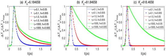
Figure 1. Changes in electron temperature $\mathsf{\Delta }{T}_e/{\left(\mathsf{\Delta }{T}_e\right)}_{max}$ and various $K_n$, $\gamma$, and $(\alpha ,\beta )=(0.999,0.999)$.

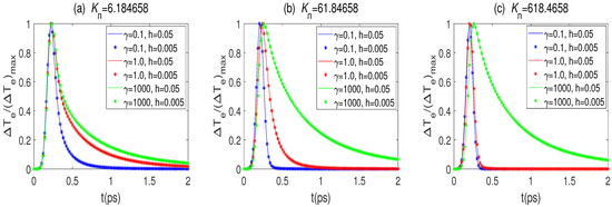
Figure 2. Changes in electron temperature $\mathsf{\Delta }{T}_e/{\left(\mathsf{\Delta }{T}_e\right)}_{max}$ and various $K_n$, $\gamma$, and $(\alpha ,\beta )=(0.9,0.9)$.

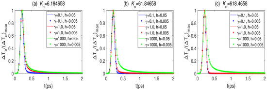
Figure 3. Changes in electron temperature $\mathsf{\Delta }{T}_e/{\left(\mathsf{\Delta }{T}_e\right)}_{max}$ and various $K_n$, $\gamma$, and $(\alpha ,\beta )=(0.5,0.5)$.

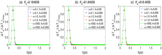
Figure 4. Changes in electron temperature $\mathsf{\Delta }{T}_e/{\left(\mathsf{\Delta }{T}_e\right)}_{max}$ and various $K_n$, $\gamma$, and $(\alpha ,\beta )=(0.1,0.1)$.

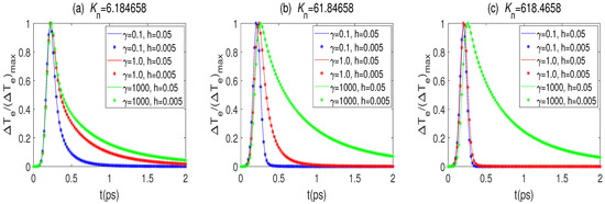
Figure 5. Changes in electron temperature $\mathsf{\Delta }{T}_e/{\left(\mathsf{\Delta }{T}_e\right)}_{max}$ and various $K_n$, $\gamma$, and $(\alpha ,\beta )=(0.9,0.3)$.

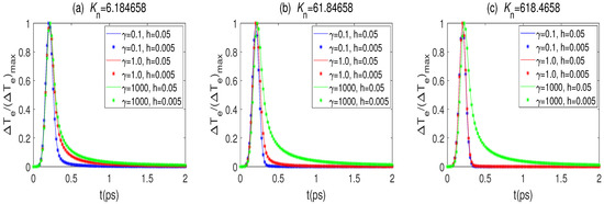
Figure 6. Changes in electron temperature $\mathsf{\Delta }{T}_e/{\left(\mathsf{\Delta }{T}_e\right)}_{max}$ and various $K_n$, $\gamma$, and $(\alpha ,\beta )=(0.6,0.4)$.

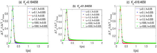
Figure 7. Changes in electron temperature $\mathsf{\Delta }{T}_e/{\left(\mathsf{\Delta }{T}_e\right)}_{max}$ and various $K_n$, $\gamma$, and $(\alpha ,\beta )=(0.3,0.9)$.

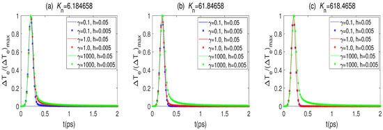
Figure 8. Changes in electron temperature $\mathsf{\Delta }{T}_e/{\left(\mathsf{\Delta }{T}_e\right)}_{max}$ and various $K_n$, $\gamma$, and $(\alpha ,\beta )=(0.4,0.6)$.

When considering the Dirichlet-like boundary condition (i.e. $\gamma =0.1$), from Figure 9 and Figure 10, the value of fractional-order $\alpha$ has a minor effect on the change in electron temperature with the fixed $\beta$, whereas, when considering the insulated boundary condition (i.e., $\gamma =1000$), one may see from Figure 11 and Figure 12 that the temperature decreases more slowly as $\alpha$ becomes large with the fixed $\beta$.

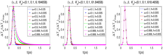
Figure 9. Changes in electron temperature $\mathsf{\Delta }{T}_e/{\left(\mathsf{\Delta }{T}_e\right)}_{max}$ and various $K_n$, $\alpha$, and $(\gamma ,\beta )=(0.1,0.1)$.

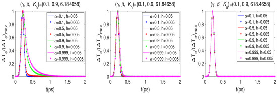
Figure 10. Changes in electron temperature $\mathsf{\Delta }{T}_e/{\left(\mathsf{\Delta }{T}_e\right)}_{max}$ and various $K_n$, $\alpha$, and $(\gamma ,\beta )=(0.1,0.9)$.

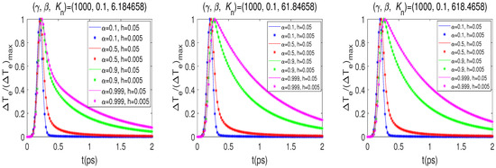
Figure 11. Changes in electron temperature $\mathsf{\Delta }{T}_e/{\left(\mathsf{\Delta }{T}_e\right)}_{max}$ and various $K_n$, $\alpha$, and $(\gamma ,\beta )=(1000,0.1)$.

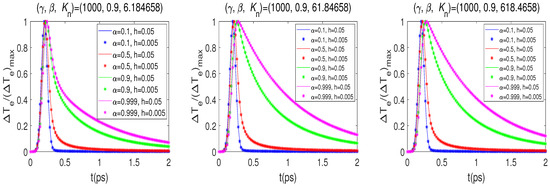
Figure 12. Changes in electron temperature $\mathsf{\Delta }{T}_e/{\left(\mathsf{\Delta }{T}_e\right)}_{max}$ and various $K_n$, $\alpha$, and $(\gamma ,\beta )=(1000,0.9)$.

Figure 13, Figure 14, Figure 15, Figure 16, Figure 17, Figure 18, Figure 19, Figure 20, Figure 21, Figure 22, Figure 23 and Figure 24 show 3D plots of temperature distributions of lattice temperature $T_l$ versus $(x,t)$ for various values of $K_n$, $\gamma$, $\alpha$ and $\beta$, respectively, which were obtained using a mesh of $N=100$ and $M=100$. When the same $\alpha$ and $\beta$ are small (see Figure 22, Figure 23 and Figure 24), $T_l$ rises quickly through the interaction between $T_e$ and $T_l$. $T_l$ rises uniformly along the x-axis through the interaction between $T_e$ and $T_l$. A similar result to that in Figure 16, Figure 17, Figure 18, Figure 19, Figure 20 and Figure 21 can be seen for the temperature $T_l$. When the same $\alpha$ and $\beta$ are large (see Figure 13, Figure 14 and Figure 15), $T_l$ rises slowly through the interaction between $T_e$ and $T_l$, and $T_l$ rises uniformly along the x-axis through the interaction between $T_e$ and $T_l$.

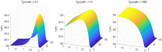
Figure 13. Temperature distributions of $T_l$ versus $(x,t)$ with various $\gamma$ when $K_n=6.184658$, $(\alpha ,\beta )=(0.9,0.9)$, $N=100$, and $M=100$ for Example 2.

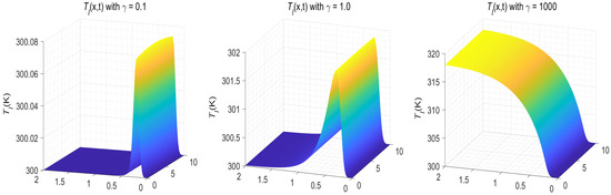
Figure 14. Temperature distributions of $T_l$ versus $(x,t)$ with various $\gamma$ when $K_n=61.84658$, $(\alpha ,\beta )=(0.9,0.9)$, $N=100$, and $M=100$ for Example 2.

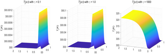
Figure 15. Temperature distributions of $T_l$ versus $(x,t)$ with various $\gamma$ when $K_n=618.4658$, $(\alpha ,\beta )=(0.9,0.9)$, $N=100$, and $M=100$ for Example 2.

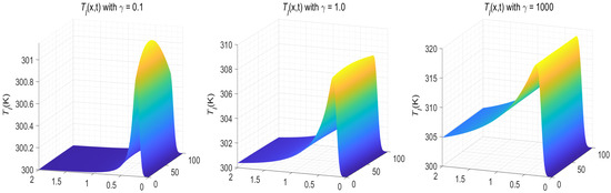
Figure 16. Temperature distributions of $T_l$ versus $(x,t)$ with various $\gamma$ when $K_n=6.184658$, $(\alpha ,\beta )=(0.8,0.3)$, $N=100$, and $M=100$ for Example 2.

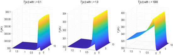
Figure 17. Temperature distributions of $T_l$ versus $(x,t)$ with various $\gamma$ when $K_n=61.84658$, $(\alpha ,\beta )=(0.8,0.3)$, $N=100$, and $M=100$ for Example 2.

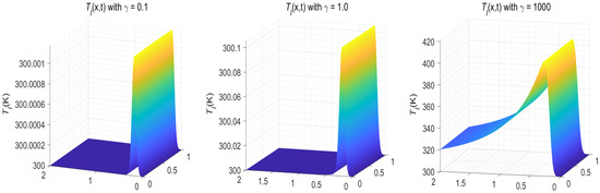
Figure 18. Temperature distributions of $T_l$ versus $(x,t)$ with various $\gamma$ when $K_n=618.4658$, $(\alpha ,\beta )=(0.8,0.3)$, $N=100$, and $M=100$ for Example 2.

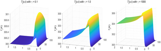
Figure 19. Temperature distributions of $T_l$ versus $(x,t)$ with various $\gamma$ when $K_n=6.184658$, $(\alpha ,\beta )=(0.3,0.8)$, $N=100$, and $M=100$ for Example 2.

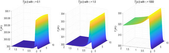
Figure 20. Temperature distributions of $T_l$ versus $(x,t)$ with various $\gamma$ when $K_n=61.84658$, $(\alpha ,\beta )=(0.3,0.8)$, $N=100$, and $M=100$ for Example 2.

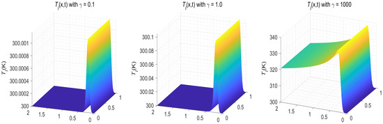
Figure 21. Temperature distributions of $T_l$ versus $(x,t)$ with various $\gamma$ when $K_n=618.4658$, $(\alpha ,\beta )=(0.3,0.8)$, $N=100$, and $M=100$ for Example 2.

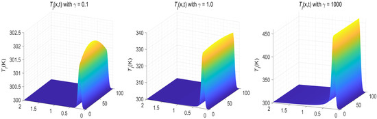
Figure 22. Temperature distributions of $T_l$ versus $(x,t)$ with various $\gamma$ when $K_n=6.184658$, $(\alpha ,\beta )=(0.1,0.1)$, $N=100$, and $M=100$ for Example 2.

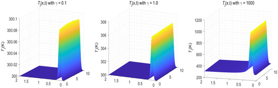
Figure 23. Temperature distributions of $T_l$ versus $(x,t)$ with various $\gamma$ when $K_n=61.84658$, $(\alpha ,\beta )=(0.1,0.1)$, $N=100$, and $M=100$ for Example 2.

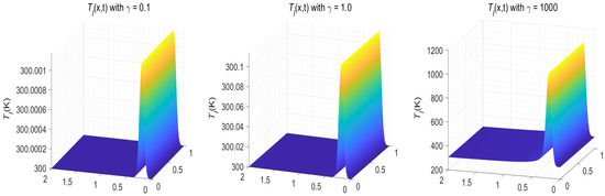
Figure 24. Temperature distributions of $T_l$ versus $(x,t)$ with various $\gamma$ when $K_n=618.4658$, $(\alpha ,\beta )=(0.1,0.1)$, $N=100$, and $M=100$ for Example 2.

6. Conclusions

In this study, we present a sub-diffusion two-temperature model by introducing the Knudsen number ($K_n$) and two Caputo fractional derivatives ($0<\alpha ,\beta <1$) in time into the parabolic two-temperature model of the diffusive type. The well posedness of the model is proved. The numerical scheme is obtained based on the $L1$ approximation for the Caputo fractional derivatives and the second-order finite difference for the spatial derivatives. The unconditional stability and convergence of the scheme are analyzed using the discrete energy method. The accuracy and the applicability of the present scheme are tested in two examples. By changing values of the Knudsen number and fractional-order derivatives as well as the parameter in the boundary condition, the simulation could be a tool for analyzing the heat conduction in porous media, such as porous thin metal films exposed to ultrashort-pulsed lasers, where the energy transports in phonon and free electron may be ultraslow at different rates.

Further research will focus on the extension of the present model and its numerical scheme to the case of three-dimensional multi-layer thin porous metal films exposed to ultrashort-pulsed lasers. The multi-layered metal thin films, for example, gold-coated metal mirrors, are often used in a high-power ultrashort pulsed laser system to avoid the problem of thermal damage since the high-power laser energy may cause thermal damage at the front surface of a single-layer film [30].

References

- Mao, Y.; Xu, M. Lattice Boltzmann numerical analysis of heat transfer in nano-scale silicon films induced by ultra-fast laser heating. Int. J. Therm. Sci. 2015, 89, 210–221. [Google Scholar]
- Khorasani, M.; Gibson, I.; Ghasemi, A.H.; Hadavi, E.; Rolfe, B. Laser subtractive and laser powder bed fusion of metals: Review of process and production features. Rapid Prototyp. J. 2023. [Google Scholar] [CrossRef]
- Tzou, D.Y.; Chen, J.K.; Beraun, J.E. Hot-electron blast induced by ultrashort-pulsed lasers in layered media. Int. J. Heat Mass Transf. 2002, 45, 3369–3382. [Google Scholar] [CrossRef]
- Qiu, T.Q.; Tien, C.L. Femtosecond laser heating of multi-layer metals-I. Analysis. Int. J. Heat Mass Transf. 1994, 37, 2789–2797. [Google Scholar] [CrossRef]
- Allu, P.; Mazumder, S. Hybrid ballistic-diffusive solution to the frequency-dependent phonon Boltzmann transport equation. Int. J. Heat Mass Transf. 2016, 100, 165–177. [Google Scholar] [CrossRef]
- Chen, J.K.; Beraun, J.E.; Tham, C.L. Investigation of thermal response caused by pulsed laser heating. Numer. Heat Transf. Part A 2003, 44, 705–722. [Google Scholar] [CrossRef]
- Bora, A.; Dai, W.; Wilson, J.P.; Boyta, J.C.; Sobolev, S.L. Neural network method for solving nonlocal two-temperature nanoscale heat conduction in gold films exposed to ultrashort-pulsed lasers. Int. J. Heat Mass Transf. 2022, 190, 122791. [Google Scholar] [CrossRef]
- Kaganov, M.I.; Lifshitz, I.M.; Tanatarov, L.V. Relaxation between electrons and crystalline lattice. Sov. Phys. JETP 1957, 4, 173–178. [Google Scholar]
- Anisimov, S.I.; Kapeliovich, B.L.; Perel’man, T.L. Electron emission from metal surfaces exposed to ultra-short laser pulses. Sov. Phys. JETP 1974, 39, 375–377. [Google Scholar]
- Qiu, T.Q.; Tien, C.L. Short-pulse laser-heating on metals. Int. J. Heat Mass Transf. 1992, 35, 719–726. [Google Scholar] [CrossRef]
- Qiu, T.Q.; Tien, C.L. Heat transfer mechanisms during short-pulse laser heating of metals. J. Heat Transf. (ASME) 1993, 115, 835–841. [Google Scholar] [CrossRef]
- Khorasani, M.; Ghasemi, A.; Leary, M.; Sharabian, E.; Cordova, L.; Gibson, I.; Downing, D.; Bateman, S.; Brandt, M.; Rolfe, B. The effect of absorption ratio on meltpool features in laser-based powder bed fusion of IN718. Opt. Laser Technol. 2022, 153, 108263. [Google Scholar] [CrossRef]
- Awad, E. On the generalized thermal lagging behavior. J. Therm. Stresses 2012, 35, 193–325. [Google Scholar] [CrossRef]
- Sherief, H.H.; EI-Sayed, A.M.A.; EI-Latief, A.M.A. Fractional order theory of thermoelasticity. Int. J. Solid Struct. 2010, 47, 269–275. [Google Scholar] [CrossRef]
- Youssef, H.M. Theory of fractional order generalized thermoelasticity. J. Heat Transfer (ASME) 2010, 132, 061301. [Google Scholar] [CrossRef]
- Yu, Y.J.; Tian, X.G.; Lu, T.J. Fractional order generalized electro-magneto-thermo-elasticity. Eur. J. Mech. A Solids 2013, 42, 188–202. [Google Scholar] [CrossRef]
- Ghazanfarian, J.; Shomali, Z.; Abbassi, A. Macro to nanoscale heat transfer: The lagging behavior. Int. J. Thermophys. 2015, 36, 1416–1467. [Google Scholar] [CrossRef]
- Ji, C.-C.; Dai, W.; Sun, Z.-Z. Numerical method for solving the time-fractional dual-phase-lagging heat conduction equation with the temperature-jump boundary condition. J. Sci. Comput. 2018, 75, 1307–1336. [Google Scholar] [CrossRef]
- Ji, C.-C.; Dai, W.; Sun, Z.-Z. Numerical schemes for solving the time-fractional dual-phase-lagging heat conduction model in a double-layered nanoscale thin film. J. Sci. Comput. 2019, 81, 1767–1800. [Google Scholar] [CrossRef]
- Ji, C.-C.; Dai, W. Numerical algorithm with fourth-order spatial accuracy for solving the time-fractional dual-phase-lagging nanoscale heat conduction equation. Numer. Math. Theor. Meth. Appl. 2023. Available online: https://www.jml.pub/intro/online/read?online_id=1928 (accessed on 2 March 2023).
- Shen, S.; Dai, W.; Cheng, J. Fractional parabolic two-step model and its numerical scheme for nanoscale heat conduction. J. Comput. Appl. Math. 2020, 345, 515–534. [Google Scholar] [CrossRef]
- Shen, S.; Dai, W.; Liu, Q.; Zhuang, P. Accurate numerical scheme for solving fractional diffusion-wave two-step model for nanoscale heat conduction. J. Comput. Appl. Math. 2023, 419, 114721. [Google Scholar]
- Mozafarifard, M.; Liao, Y.; Nian, Q.; Wang, Y. Two-temperature time-fractional model for electron-phonon coupled interfacial thermal transport. Int. Heat Mass Transf. 2023, 202, 123759. [Google Scholar] [CrossRef]
- Podlubny, I. Fractional Differential Equations; Academic Press: New York, NY, USA, 1999. [Google Scholar]
- Ghazanfarian, J.; Abbassi, A. Effect of boundary phonon scattering on dual-phase-lag model to simulate micro- and nano-scale heat conduction. Int. J. Heat Mass Transf. 2009, 52, 3706–3711. [Google Scholar] [CrossRef]
- Sun, Z.-Z. Numerical Methods for Partial Differential Equations, 2nd ed.; Science Press: Beijing, China, 2012. [Google Scholar]
- López-Marcos, J.C. A difference scheme for a nonlinear partial integrodifferential equation. SIAM J. Numer. Anal. 1990, 27, 20–31. [Google Scholar]
- Tzou, D.Y. Macro to Micro Scale Heat Transfer: The Lagging Behavior, 2nd ed.; Wiley: New York, NY, USA, 2015. [Google Scholar]
- Kaba, I.K.; Dai, W. A stable three-level finite difference scheme for solving the parabolic two-step model in a 3D micro-sphere heated by ultrashort-pulsed lasers. J. Comput. Appl. Math. 2005, 181, 125–147. [Google Scholar] [CrossRef]
- Tsai, T.W.; Lee, Y.M. Analysis of microscale heat transfer and ultrafast thermoelasticity in a multi-layered metal film with nonlinear thermal boundary resistance. Int. J. Heat Mass Transf. 2013, 62, 87–98. [Google Scholar] [CrossRef]
Disclaimer/Publisher’s Note: The statements, opinions and data contained in all publications are solely those of the individual author(s) and contributor(s) and not of MDPI and/or the editor(s). MDPI and/or the editor(s) disclaim responsibility for any injury to people or property resulting from any ideas, methods, instructions or products referred to in the content. |
© 2023 by the authors. Licensee MDPI, Basel, Switzerland. This article is an open access article distributed under the terms and conditions of the Creative Commons Attribution (CC BY) license (https://creativecommons.org/licenses/by/4.0/).