Image Edge Detection Based on Fractional-Order Ant Colony Algorithm

Abstract

Edge detection is a highly researched topic in the field of image processing, with numerous methods proposed by previous scholars. Among these, ant colony algorithms have emerged as a promising approach for detecting image edges. These algorithms have demonstrated high efficacy in accurately identifying edges within images. For this paper, due to the long-term memory, nonlocality, and weak singularity of fractional calculus, fractional-order ant colony algorithm combined with fractional differential mask and coefficient of variation (FACAFCV) for image edge detection is proposed. If we set the order of the fractional-order ant colony algorithm and fractional differential mask to $v=0$, the edge detection method we propose becomes an integer-order edge detection method. We conduct experiments on images that are corrupted by multiplicative noise, as well as on an edge detection dataset. Our experimental results demonstrate that our method is able to detect image edges, while also mitigating the impact of multiplicative noise. These results indicate that our method has the potential to be a valuable tool for edge detection in practical applications.

1. Introduction

Edges can be defined as sets of pixels located in regions of an image that exhibit pronounced changes in intensity and correspond to discernible contour characteristics of objects depicted in the image. The objective of performing edge detection on an image is to retrieve information pertaining to its edges from the source. In general terms, a grayscale image is typically used as the input for performing image edge detection. The result of image edge detection typically is a binary image that contains discrete edge information. This binary image represents edges as a composition of black and white pixels, commonly referred to as an “edge image”. Image edge detection is a critical technology in the field of digital image processing. This technique is applied in various domains such as fingerprint detection [1,2,3], face recognition [4,5,6], image segmentation [7,8,9,10], and more. Hence, the precision of edge detection is a crucial aspect of applications that rely on edge detection. At present, many basic edge detection techniques rely heavily on the gradient information of an image. As an illustration, the Sobel [11], Prewitt [12], and Roberts [13] techniques are based on first-order differentiation, whereas the Log [14] algorithm is based on second-order differentiation. Additionally, the Canny [15] algorithm also employs differential method in its implementation. In addition to the above methods, the application of the ant colony algorithm in image edge detection has gained prominence in recent years. This is mainly attributed to the fact that image edges can be viewed as regions where there is a considerable variance in gray values, which can be efficiently identified using the ant colony algorithm.

Ant colony optimization (ACO) [16] is a heuristic optimization approach that draws inspiration from the foraging behavior of ants in nature. It is designed to solve optimization problems by simulating the search for food by ants and their communication behavior using pheromones. ACO algorithms can be broadly classified into two main categories based on the use of integer or fractional calculus for implementing the transition probability or pheromone update criteria. The first category of ACO algorithms comprises integer calculus, including the ant system (AS) [17] and ant colony system (ACS) [18] developed by Dorigo, as well as the MAX–MIN ant system (MMAS) [19] proposed by Thomas Stützle, and more. The second category of ACO algorithms comprises fractional calculus. Pu et al. [20] incorporated fractional calculus into the ant colony algorithm. Pu’s experimental findings demonstrated that the fractional-order ant colony algorithm (FACA) outperformed the integer-order ant colony algorithm (IACA). However, it was also noted that the time complexity of the algorithm was high, which was a potential issue. Gong et al. [21] proposed a hybrid algorithm based on a state-adaptive slime mold model and fractional-order ant system (SSMFAS). Experimental results showed that the method was superior to the integer-order methods. Zhu et al. [22] introduced fractional-order memristive ant colony algorithm (FMAC), which was implemented on fractional-order memristors to improve the performance. The experiments further illustrated the benefits of utilizing fractional-order methods in comparison to integer-order methods. From the aforementioned facts, it can be observed that the majority of fractional-order techniques outperform their integer-order counterparts.

Image edge detection using ant colony algorithm was initially introduced by Nezamabadi-pour et al. [23] The overall concept involved the random distribution of ants across the pixels of the image. The ants’ movement was guided by transition probability, and they deposited pheromones as they traveled, which were also referred to as trail markings. Once the algorithm was completed, a pheromone matrix was generated. By applying a threshold to the pheromone matrix, an edge image was obtained in the form of a binary image. The author’s experimental findings demonstrated that this approach effectively detected the image edges. Tian et al. [24] employed various analytical functions to initialize the heuristic function and investigated how the heuristic function affected the output of the algorithm. The experimental data indicated that the heuristic function played a critical role in determining the output results. Etemad et al. [25] delegated the decision-making authority of transition probability to pheromones, which was initialized using the gradient information. They applied this approach to process images containing salt-and-pepper noise, and their experimental findings demonstrated its superiority over other edge detection methods such as Sobel, Canny, Prewitt, and Log. When it came to image without noise, the effectiveness of its algorithm could be considered to be somewhere between the Sobel and Prewitt operators on one end, and the Canny and Log operators on the other end. Liu et al. [26] introduced a novel approach to initialize the heuristic function using the integer-order gradient. A comprehensive examination of the influence of various parameters on ant colony algorithm for edge detection was carried out. Furthermore, they applied their method to images corrupted by Gaussian noise and compared their results with those obtained by Nezamabadi-pour et al. and Tian et al. Moreover, they evaluated the performance of their approach against that of conventional edge detection operators, and the findings suggested that their algorithm exhibited strong robustness. The majority of the heuristic functions or pheromones used in the aforementioned algorithms are initialized with the gradient information derived from images. Subsequently, several scholars suggested initializing the heuristic function using statistical information extracted from an image. Martínez et al. [27] initialized the heuristic function using a combination of mean and variance and compared its performance with Canny and gPb on images contaminated with Gaussian and salt-and-pepper noise. The results indicated that their approach exhibited robustness to noise. Furthermore, it demonstrated superior performance over certain aforementioned algorithms when applied to noise-free images. Sergio Baltierra et al. [28] initialized the heuristic function using the coefficient of variation (CV) or gradient to conduct experiments on images corrupted with multiplicative noise, which could severely degrade image quality. The findings indicated that the method based on the coefficient of variation was effective in mitigating the impact of noise on edge detection. However, under a high level of noise, the algorithm might cause edge image distortion. Based on the aforementioned facts, ant colony algorithm can effectively detect edges. Furthermore, it is evident that the ant colony algorithm based on statistical information of an image mostly surpasses the gradient-based method. However, at present, all methods for edge detection based on ant colony algorithm are integer-order methods that utilize IACA. In this paper, we aim to incorporate FACA into edge detection.

The theories of fractional calculus and integer calculus emerged almost simultaneously, with fractional calculus being an extension of integer calculus theory. Fractional calculus is characterized by long-term memory, non-locality, and weak singularity [29].In recent years, fractional-order methods have achieved important applications in the field of engineering, attracting more and more scholars. Research interests in the field of fractional calculus include various topics such as fractional-order image processing [30,31,32], fractional-order control theory [33,34], and fractional-order digital signal processing [35,36]. In the image processing domain, using integer-order operators can enhance the high-frequency portion of the image but also cause information loss in the low-frequency portion. Pu et al. [37] proposed six types of multiscale fractional differential masks. Theoretical analysis and results indicated that the proposed multiscale fractional differential operator had better performance than the traditional integer-order operator in preserving the information of low-frequency portion while enhancing the high-frequency portion in image processing.

Based on the aforementioned background, it is evident that previous research utilizes IACA for edge detection. Fractional calculus exhibits characteristics such as long-term memory, non-locality, and weak singularity. Therefore, exploring the applicability of FACA for image edge detection constitutes a promising area of research. Motivated by this need, fractional calculus is used to ameliorate integer-order ant colony algorithm combined with coefficient of variation (IACACV) for image edge detection in the literature [28]. As a result, fractional-order ant colony algorithm combined with fractional differential mask and coefficient of variation (FACAFCV) for image edge detection is obtained.

The text is structured as follows:

(a)

Section 2 provides an overview of fractional calculus, including its fundamental definition. Additionally, this section introduces the fundamental principles and procedures of the fractional-order ant colony algorithm.

(b)

In Section 3, a novel edge detection technique utilizing the fractional-order ant colony algorithm combined with fractional differential mask and coefficient of variation (FACAFCV) is presented. The heuristic function utilized in this approach is constructed by amalgamating the concepts of fractional differential mask and the coefficient of variation (CV).

(c)

In Section 4, a reasonable experimental strategy is designed to evaluate the results of edge detection on images with and without noise, using metrics such as recall, precision, and F-measure.

(d)

Section 5 performs a comprehensive analysis of our method through three distinct experiments. Firstly, the impact of the fractional differential mask and coefficient of variation on the edge detection performance is examined. Secondly, the performance of both fractional-order ant colony algorithm combined with fractional differential mask and coefficient of variation (FACAFCV) and fractional-order ant colony algorithm combined with coefficient of variation (FACACV) in the presence of multiplicative noise is studied. Finally, a standard benchmark evaluation is carried out on the widely-used dataset to assess the effectiveness of the proposed method.

(e)

Section 6 delves into the merits and limitations of our method, as well as future research directions. Furthermore, potential applications of our method are outlined.

2. Background

2.1. Fractional Calculus

In the realm of Euclidean measure, the widely adopted fractional calculus definitions are those of Grünwald-Letnikov [29], Riemann-Liouville [38], and Caputo [39]. These definitions are extensively employed in research and applications in related fields, providing the foundation and support for theoretical investigation and practical utilization of fractional calculus. The Grünwald-Letnikov definition is selected in this work not only because of its simplicity in form but also due to its feasibility for implementation. For a causal function $f(x)$, the Grünwald-Letnikov definition of fractional calculus of order v, in a form that is amenable for practical application, can be rendered as:

$${}_a^{G-L}{D}_x^{v}f(x)=\underset{N\to \infty }{\lim }\left\{\frac{{\left(\frac{x-a}{N}\right)}^{-v}}{\Gamma (-v)}{\displaystyle \sum _{k=0}^{N-1}\frac{\Gamma (k-v)}{\Gamma (k+1)}f\left[x-k\left(\frac{x-a}{N}\right)\right]}\right\},$$

(1)

where ${}_a^{G-L}{D}_x^v$ is a fractional differential operator based on Grünwald-Letnikov definition, $[a,x]$ is the domain of $f(x)$, $v$ is a non-integer, $f(x)$ is a differintegrable function [29], $\Gamma (-v)={\displaystyle \underset{0}{\overset{\infty }{\int }}{e}^{-x}{x}^{-v-1}dx}$ is a Gamma function, and $(x-a)/N$ is an interval of $[a,x]$. Let $\Delta x=(x-a)/N$. From (1), the Grünwald-Letnikov definition of fractional forward difference can be expressed as:

$$\begin{array}{cc}\hfill {}_a^{G-L}{Diff}_x^v& f(x)=\frac{1}{{(\Delta x)}^v}{\displaystyle \sum _{k=0}^{N-1}\frac{\Gamma (k-v)}{\Gamma (-v)\Gamma (k+1)}}f(x-k\Delta x)\hfill \\ & =\frac{1}{{(\Delta x)}^v}\left[f(x)+{\displaystyle \sum _{k=1}^{N-1}\frac{\Gamma (k-v)}{\Gamma (-v)\Gamma (k+1)}}f(x-k\Delta x)\right]\hfill \end{array},$$

(2)

where ${}_a^{G-L}Dif{f}_x^v$ is a fractional forward difference operator. When $v=1$ in (2), the first-order forward difference can be derived as:

$${}_{a}Dif{f}_x^{1}f(x)=\frac{1}{\Delta x}\left[f(x)-f(x-\Delta x)\right].$$

(3)

In (2), the absolute fractional forward difference can be derived when the coefficient in front of $f(x-k\Delta x)$ is $\left|\frac{\Gamma (k-v)}{\Gamma (-v)\Gamma (k+1)}\right|$. It is not difficult to observe that $\left|\frac{\Gamma (k-v)}{\Gamma (-v)\Gamma (k+1)}\right|$ is a decreasing function about $k$. By using Equations (1) and (2), we can obtain the three fundamental properties, namely long-term memory, non-locality, and weak singularity, which are compared with Equation (3). These properties are attributed to the ability of Equations (1) and (2) to contain a significant amount of forward information and the fact that the fractional derivative of a constant (non-zero) is not zero.

2.2. Fractional-Order Ant Colony Algorithm (FACA)

Pu et al. initially extended the concept of IACA to FACA, with the fundamental principles of FACA originating from fractional calculus. By applying the principles of fractional calculus, the characteristics of IACA can be fully optimized to encompass long-term memory, non-locality, and weak singularity. In this section, since IACA is a special case of FACA, we will provide an overview of FACA. The transition probability for the $m$th ant at the $t$th iteration can be calculated as follows:

$${}^{m}p_{i j}^v(t)=\frac{1}{f}\left\{\begin{array}{l}{p}_{i j}(t)+{\displaystyle \sum _{k=1}^{N_1-1}\left|\frac{\Gamma (k-v)}{\Gamma (-v)\Gamma (k+1)}\right|p_{(j+k-1)(j+k)}(t)\hspace{1em}if j\in C_i^m(t) and (j+k})\in C_i^m(t)\hfill \\ 0\hspace{1em}\hspace{1em}\hspace{1em}if j\notin C_i^m(t) \hfill \end{array}\right.,$$

(4)

where $f={\displaystyle \sum _{k=0}^{N_1-1}\left|\frac{\Gamma (k-v)}{\Gamma (-v)\Gamma (k+1)}\right|}$ is a normalization factor, $0\le {}^{m}p_{i j}^v(t)\le 1$, $C_i^m(t)$ is the set of neighboring nodes connected to node $i$ that represent the potential next nodes to be traversed, $N_1-1$ is the quantity of the set $C_i^m(t)$, ${}^{m}p_{i j}^v(t)$ is the fractional-order transition probability of order $v$ for the $m$th ant, which contains a series of information $p_{(j+k-1)(j+k)}(t)$ composed of adjacent edges neighboring edge $(i,j)$, and $p_{(j+k-1)(j+k)}(t)$ represents a series of future transition probabilities. $p_{i j}(t)$ and $p_{(j+k-1)(j+k)}(t)$ can be given as:

$$p_{i j}(t)=\left\{\begin{array}{l}\frac{{[{\tau }_{i j}(t)]}^{\alpha }{[{\eta }_{i j}(t)]}^{\beta }}{{\displaystyle \sum _{c\in C_i^m(t)}}{[{\tau }_{i c}(t)]}^{\alpha }{[{\eta }_{i c}(t)]}^{\beta }}\hspace{1em}if\hspace{0.17em}j\in C_i^m(t)\hfill \\ 0\hspace{1em}\hspace{1em}if\hspace{0.17em}j\notin C_i^m(t)\hfill \end{array}\right.,$$

(5)

$$p_{\left(j+k-1\right)\left(j+k\right)}(t)=\left\{\begin{array}{l}\frac{{[{\tau }_{\left(j+k-1\right)\left(j+k\right)}(t)]}^{\alpha }{[{\eta }_{\left(j+k-1\right)\left(j+k\right)}(t)]}^{\beta }}{{\displaystyle \sum _{c\in C_{\left(j+k-1\right)}^m(t)}}{[{\tau }_{\left(j+k-1\right)c}(t)]}^{\alpha }{[{\eta }_{\left(j+k-1\right)c}(t)]}^{\beta }}\hspace{1em}if\hspace{0.17em}(j+k)\in C_{(j+k-1)}^m(t)\hfill \\ 0\hspace{1em}\hspace{1em}if\hspace{0.17em}(j+k)\notin C_{(j+k-1)}^m(t)\hfill \end{array}\right.,$$

(6)

where $0\le p_{i j}(t)\le 1$, $0\le p_{(j+k-1)(j+k)}(t)\le 1$, $\alpha$ is the weight of pheromone concentration, $\beta$ is the weight of heuristic information, ${\eta }_{i j}(t)$ is the heuristic information, which is initialized with $1/d_{i j}$, where $d_{i j}=\sqrt{{(x_i-x_j)}^2+{(y_i-y_j)}^2}$ is the Euclidean distance. When $v=0$, Equation (4) becomes the classical transition probability. In order to avoid falling into local optima, we need to implement strategies to promote exploration. The group of subsequent nodes linked to the $i$th node in Equation (4), $S_i^m(t)\subset C_i^m(t)$, can be expressed as:

$$\left\{\begin{array}{l}j\hspace{1em}\hspace{1em}if p_{i j}^m=\max \left[{}^m{p}_{i c}^v(t)\right] ,j and c\in C_i^m(t)\hfill \\ l\hspace{1em}\hspace{1em}if d_{i l}(t)\le \xi d_{i j}(t) ,l and j\in C_i^m(t)\hfill \\ \varphi \hspace{1em}\hspace{1em}otherwise\hfill \end{array}\right\}\in S_i^m(t),$$

(7)

where $p_{i j}^m$ is maximum probability of fractional-order transition probability ${}^m{p}_{i c}^v(t)$, $\xi \in [1,2]$ is a relaxation coefficient, $\varphi$ denotes null set, $N_2=\left|S_i^m(t)\right|$ is the number of elements in set $S_i^m(t)$. Let $\theta$ equal the number of $\max \left[{}^m{p}_{i c}^v(t)\right]$. The $m$th ant clones itself to other $(N_2-\theta )$ ants to visit the rest of the nodes. However, the total number of ants is limited to $Q_p$, and the initial number of ants is $Q_a$. The first and the second if-cases are not mutually exclusive. Prior to presenting the pheromone update criteria, we need to sort the ants by the length of their tours and select the top $N_3$ ants with the shortest tour length as the elite ants. Then, the pheromone update criteria can be given as:

$${\tau }_{i j}(t+1)=(1-\rho ){\tau }_{i j}(t)+{\displaystyle \sum _{m=1}^{N_3}\left|\frac{\Gamma (m-v-1)}{\Gamma (-v)\Gamma (m)}\right|}\Delta {\tau }_{i j}^m(t),$$

(8)

where $0<\rho <1$ is the pheromone volatilization rate and $\Delta t=1$. $\Delta \tau$ is the increment of pheromone. ${\tau }_{i j}$ is constrained within the range $\left[{\tau }_{min},{\tau }_{max}\right]$. $N_3$ represents the number of elitist ants in an iteration. When the coefficient before $\Delta {\tau }_{i j}^m(t)$ is 1, Equation (8) becomes the classical pheromone update criteria. $\Delta \tau$ is given as:

$$\Delta {\tau }_{i j}^m(t)=\left\{\begin{array}{l}\frac{1}{L^m(t)}\hspace{1em}if the mth elitist ant visited edge (i,j) \hfill \\ 0\hspace{1em}\hspace{1em} if the mth elitist ant doesn’t visit edge (i,j) \hfill \end{array}\right.,$$

(9)

where $L^m(t)$ is the distance of the $m$th ant in iteration $t$. Once again, (8) exhibits properties of long-term memory, non-locality, and weak singularity of fractional calculus. In summary, when $v=0$ in (4) and the coefficient before $\Delta {\tau }_{i j}^m(t)$ is 1 in (8), Equations (4) and (8) become the traditional integer-order transition probability and pheromone update criteria. Thus, IACA is a special case of FACA.

3. Fractional-Order Ant Colony Algorithm Combined with Fractional Differential Mask and Coefficient of Variation (FACAFCV) for Image Edge Detection

In this section, fractional-order ant colony algorithm combined with fractional differential mask and coefficient of variation (FACAFCV) for image edge detection is proposed by using fractional calculus. In contrast to the traveling salesman problem (TSP), where the objective is to find the shortest route that visits a set of cities and returns to the starting point, an individual pixel in an image is typically represented by $(i,j)$. At the outset, the ants’ locations are initially randomized and situated above the mean value of the grayscale alterations. When the ant is on the pixel $(r,s)$, the transition probability for the $m$th ant at the $t$th iteration can be calculated as follows:

$$\begin{array}{l}{}^{m}p_{(r,s)(i,j)}^v(t)=\\ \frac{1}{f}\left\{\begin{array}{l}\begin{array}{l}{p}_{(r,s)(i,j)}(t)+\\ {\displaystyle \sum _{k=1}^{N_1-1}\left|\frac{\Gamma (k-v)}{\Gamma (-v)\Gamma (k+1)}\right|p_{(r,s)(i+k,j+k)}(t)\hspace{1em}if (i,j) \in {\Omega }_{(r,s)}^m(t) and (i+k,j+k})\in {\Omega }_{(r,s)}^m(t) \end{array}\hfill \\ \begin{array}{l}\\ 0\hspace{1em}\hspace{1em}if (i,j)\notin {\Omega }_{(r,s)}^m(t) \end{array}\hfill \end{array}\right.\end{array},$$

(10)

where $f={\displaystyle \sum _{k=0}^{N_1-1}\left|\frac{\Gamma (k-v)}{\Gamma (-v)\Gamma (k+1)}\right|}$ is a normalization factor, $0\le {}^{m}p_{(r,s)(i,j)}^v(t)\le 1$, and ${\Omega }_{(r,s)}^m(t)$ is the set of neighboring pixels connected to pixel $(r,s)$ that represent the potential next pixels in 8-connectivity neighborhood shown in Figure 1 to be traversed,

$N_1-1$ is the quantity of the set ${\Omega }_{(r,s)}^m(t)$, ${}^{m}p_{(r,s)(i,j)}^v(t)$ is the fractional-order transition probability of order $v$ for the $m$th ant, which contains a series of information $p_{(r,s)(i+k,j+k)}(t)$ composed of adjacent pixels neighboring pixel $(r,s)$. When $v=0$, Equation (10) becomes the classical transition probability. $p_{(r,s)(i,j)}(t)$ and $p_{(r,s)(i+k,j+k)}(t)$ can be given as:

$$p_{(r,s)(i,j)}(t)=\left\{\begin{array}{l}\frac{{[{\tau }_{(i,j)}(t)]}^{\alpha }{[{\eta }_{ (i,j)}(t)]}^{\beta }}{{\displaystyle \sum _{(u,z)\in {\Omega }_{(r,s)}^m(t)}}{[{\tau }_{(u,z)}(t)]}^{\alpha }{[{\eta }_{(u,z)}(t)]}^{\beta }}\hspace{1em}\hspace{1em}if\hspace{0.17em}(i,j)\in {\Omega }_{(r,s)}^m(t)\hfill \\ 0\hspace{1em}\hspace{1em}\hspace{1em}if\hspace{0.17em}(i,j)\notin {\Omega }_{(r,s)}^m(t)\hfill \end{array}\right.,$$

(11)

$$p_{\left(r,s\right)\left(i+k,j+k\right)}(t)=\left\{\begin{array}{l}\frac{{[{\tau }_{\left(i+k,j+k\right)}(t)]}^{\alpha }{[{\eta }_{\left(i+k,j+k\right)}(t)]}^{\beta }}{{\displaystyle \sum _{(u,z)\in {\Omega }_{(r,s)}^m(t)}}{[{\tau }_{\left(u,z\right)}(t)]}^{\alpha }{[{\eta }_{\left(u,z\right)}(t)]}^{\beta }}\hspace{1em}\hspace{1em}if\hspace{0.17em}\left(i+k,j+k\right)\in {\Omega }_{(r,s)}^m(t)\hfill \\ 0\hspace{1em}\hspace{1em}\hspace{1em}if\hspace{0.17em}\left(i+k,j+k\right)\notin {\Omega }_{(r,s)}^m(t)\hfill \end{array}\right.,$$

(12)

where $0\le p_{(r,s)(i,j)}(t)\le 1$, $0\le p_{(r,s)(i+k,j+k)}(t)\le 1$, $\alpha$ is the weight of pheromone concentration, $\beta$ is the weight of heuristic information, ${\eta }_{(i,j)}(t)$ is the heuristic function at pixel $(i,j)$. ${\eta }_{(i,j)}(t)$ is initialized with fractional differential mask and CV. The PU-2 operator [37] is obtained through the utilization of the Grünwald-Letnikov formula in conjunction with the Lagrange interpolation formula. The backward difference of fractional partial differential respectively on negative x- and y-coordinate can be obtained as:

$$\begin{array}{cc}\hfill \frac{{\partial }^{v}f(x,y)}{\partial x^v}& \cong \left(\frac{v}{4}+\frac{v^2}{8}\right)f(x+1,y)+\left(1-\frac{v^2}{2}-\frac{v^3}{8}\right)f(x,y)\hfill \\ \hfill & +\frac{1}{\Gamma (-v)}{\displaystyle \sum _{k=1}^{n-2}\left[\frac{\Gamma (k-v+1)}{(k+1)!}\left(\frac{v}{4}+\frac{v^2}{8}\right)+\frac{\Gamma (k-v)}{k!}\left(1-\frac{v^2}{4}\right)+\frac{\Gamma (k-v-1)}{(k-1)!}\left(-\frac{v}{4}+\frac{v^2}{8}\right)\right]}f(x-k,y)\hfill \\ \hfill & +\left[\frac{\Gamma (n-v-1)}{(n-1)!\Gamma (-v)}\left(1-\frac{v^2}{4}\right)+\frac{\Gamma (n-v-2)}{(n-2)!\Gamma (-v)}\left(-\frac{v}{4}+\frac{v^2}{8}\right)\right]f(x-n+1,y)\hfill \\ \hfill & +\frac{\Gamma (n-v-1)}{(n-1)!\Gamma (-v)}\left(-\frac{v}{4}+\frac{v^2}{8}\right)f(x-n,y)\hfill \end{array},$$

(13)

$$\begin{array}{cc}\hfill \frac{{\partial }^{v}f(x,y)}{\partial y^v}& \cong \left(\frac{v}{4}+\frac{v^2}{8}\right)f(x,y+1)+\left(1-\frac{v^2}{2}-\frac{v^3}{8}\right)f(x,y)\hfill \\ \hfill & +\frac{1}{\Gamma (-v)}{\displaystyle \sum _{k=1}^{n-2}\left[\frac{\Gamma (k-v+1)}{(k+1)!}\left(\frac{v}{4}+\frac{v^2}{8}\right)+\frac{\Gamma (k-v)}{k!}\left(1-\frac{v^2}{4}\right)+\frac{\Gamma (k-v-1)}{(k-1)!}\left(-\frac{v}{4}+\frac{v^2}{8}\right)\right]}f(x,y-k)\hfill \\ \hfill & +\left[\frac{\Gamma (n-v-1)}{(n-1)!\Gamma (-v)}\left(1-\frac{v^2}{4}\right)+\frac{\Gamma (n-v-2)}{(n-2)!\Gamma (-v)}\left(-\frac{v}{4}+\frac{v^2}{8}\right)\right]f(x,y-n+1)\hfill \\ \hfill & +\frac{\Gamma (n-v-1)}{(n-1)!\Gamma (-v)}\left(-\frac{v}{4}+\frac{v^2}{8}\right)f(x,y-n)\hfill \end{array},$$

(14)

Upon obtaining the backward difference of fractional partial differential, it is possible to apply a convolution filter respectively on the above 8 directions from the current pixel by using PU-2 operator in $5\times 5$ mask, which can be given as:

$$G=\frac{{\displaystyle \sum _{i=1}^8}\frac{{\partial }^{v}I}{\partial x_i{}^v}}{S},$$

(15)

where $I$ is the image to be processed, $\frac{{\partial }^{v}I}{\partial x_i{}^v}(i=1,2,3,\cdots ,8)$ is employed to perform fractional differentiation of the eight directions $(0^{°},{45}^{°},{90}^{°},{135}^{°},{180}^{°},{225}^{°},{270}^{°},{315}^{°})$ of the current pixel, $S$ is a normalization factor, which can be given as:

$$\begin{array}{cc}\hfill S=& \left(\frac{v}{4}+\frac{v^2}{8}\right)+\left(1-\frac{v^2}{2}-\frac{v^3}{8}\right)\hfill \\ \hfill & +\frac{1}{\Gamma (-v)}\left[\frac{\Gamma (2-v)}{2!}\left(\frac{v}{4}+\frac{v^2}{8}\right)+\frac{\Gamma (1-v)}{1!}\left(1-\frac{v^2}{4}\right)+\frac{\Gamma (-v)}{0!}\left(-\frac{v}{4}+\frac{v^2}{8}\right)\right]\hfill \\ \hfill & +\left[\frac{\Gamma (2-v)}{2!\Gamma (-v)}\left(1-\frac{v^2}{4}\right)+\frac{\Gamma (1-v)}{1!\Gamma (-v)}\left(-\frac{v}{4}+\frac{v^2}{8}\right)\right]\hfill \\ \hfill & +\frac{\Gamma (2-v)}{2!\Gamma (-v)}\left(-\frac{v}{4}+\frac{v^2}{8}\right)\hfill \end{array},$$

(16)

After applying fractional differentiation to the entire image, the original pixel information is preserved. As a result, the initialization of the heuristic function can be accomplished by calculating the CV of the masked image. CV can be given as:

$$\eta =CV(G)=\frac{\sigma }{\mu },$$

(17)

where $\sigma$ is the standard deviation and $\mu$ is the mean value. $\sigma$ and $\mu$ can be given as:

$$\mu =\frac{1}{M\times N}{\displaystyle \sum _{i=1}^M{\displaystyle \sum _{j=1}^{N}G(i,j)}},$$

(18)

$$\sigma =\sqrt{\frac{1}{M\times N}{\displaystyle \sum _{i=1}^M{\displaystyle \sum _{j=1}^N{\left[G(i,j)-\mu \right]}^2}}},$$

(19)

where $M\times N$ is the size of the 8-connectivity neighborhood. First, if the $v$ of the fractional differential mask is equal to 0, the heuristic function is initialized using the coefficient of variation, as proposed in the literature [28]. This indicates that the heuristic function initialization method in the literature [28] is a special case of our method, and consequently, FACAFCV becomes FACACV. Second, $p_{(r,s)(i+k,j+k)}(t)$ represents a series of neighbor transition probabilities. The probability of transition for a particular pixel pertains to its present rather than future transition probability. The computation of the future probability of transition is time-consuming; hence, using the current probability of transition can expedite the calculation and facilitate rapid outcome acquisition. Third, it is reasonable to argue that $\left|\frac{\Gamma (k-v)}{\Gamma (-v)\Gamma (k+1)}\right|$ demonstrates a consistently decreasing trend in relation to $k$. This implies that as the degree of grayscale fluctuations in images decreases, the significance of the information conveyed by $\left|\frac{\Gamma (k-v)}{\Gamma (-v)\Gamma (k+1)}\right|$ also decreases. Fourth, to avoid falling into a local optimum during the search for pixels, every ant possesses a memory length and a maximum distance $L$ that it can traverse. Fifth, when the number of selectable pixels is fewer than three, the algorithm generates a new random location to access the remaining pixels, thus promoting exploration and avoiding premature convergence. Moreover, we need to implement strategies to promote exploration and prevent premature convergence. The group of subsequent pixels linked to the pixel $(r,s)$ in Equation (10), $S_{(r,s)}^m(t)\subset {\Omega }_{(r,s)}^m(t)$, can be expressed as:

$$\left\{\begin{array}{l}(i.j)\hspace{1em}\hspace{1em}if p_{(r,s)(i.j)}^m=\left[th\le \frac{{}^m{p}_{(r,s)(u,z)}^v(t)}{\max \left[{}^m{p}_{(r,s)(u,z)}^v(t)\right]}\right] ,(i,j) and (u,z)\in {\Omega }_{(r,s)}^m(t)\hfill \\ l\hspace{1em}\hspace{1em}\hspace{1em} if {\eta }_{(u,z)}(t)\le \xi {\eta }_{(i,j)}(t) ,(i,j) and (u,z)\in {\Omega }_{(r,s)}^m(t)\hfill \\ \varphi \hspace{1em}\hspace{1em}\hspace{1em} otherwise\hfill \end{array}\right\}\in S_{(r,s)}^m(t),$$

(20)

where $th\in \left(0,1\right)$, ${\Omega }_{(r,s)}^m(t)$ represents the 8-connectivity neighborhood of the current pixel, $\varphi$ is an empty set, $\xi \in [1,2]$ is a loose coefficient, $N_2=\left|S_{(r,s)}^m(t)\right|$ is the number of elements in set $S_{(r,s)}^m(t)$. To enhance the exploratory capacity of ants, it is possible to clone them within a loosely defined range of coefficients to promote greater diversity in the search for pixels. In accordance with the resolution of the TSP, once the first criterion has been met, a pixel $(i,j)$ should be chosen for accessibility. Let $\theta$ equal the number of $\left[th\le \frac{{}^m{p}_{(r,s)(u,z)}^v(t)}{\max \left[{}^m{p}_{(r,s)(u,z)}^v(t)\right]}\right]$. The $m$th ant clones itself to other $(N_2-\theta )$ ants to visit the rest of the pixels. However, the total number of ants is limited to $Q_p$ and the initial number of ants is $Q_a$. The first and the second if-case are not mutually exclusive. Then, the pheromone update criteria can be given as:

$${\tau }_{(i,j)}(t+1)=(1-\rho ){\tau }_{(i,j)}(t)+{\displaystyle \sum _{m=1}^{N_3}\Delta {\tau }_{(i,j)}^m(t)},$$

(21)

where $0<\rho <1$ is the pheromone volatilization rate and $\Delta t=1$, $\Delta \tau$ is the increment of pheromone, ${\tau }_{(i,j)}$ is constrained within the range $\left[{\tau }_{min},{\tau }_{max}\right]$, the initial value of the pheromone is ${\tau }_0$, and $N_3$ represents the number of ants in the FACAFCV. In contrast to previous method, the route taken by each ant is now utilized for updating pheromone information in edge detection. $\Delta \tau$ is given as:

$$\Delta {\tau }_{(i,j)}^m(t)=\left\{\begin{array}{l}{\eta }_{(i,j)}\hspace{1em}\hspace{1em}if the mth ant visited pixel (i,j) \hfill \\ 0\hspace{1em}\hspace{1em}\hspace{1em}if the mth ant doesn’t visit pixel (i,j) \hfill \end{array}\right.,$$

(22)

where ${\eta }_{(i,j)}$ is the value of the heuristic function. Limiting the distribution of pheromones can serve as a preventative measure against ants becoming trapped in local optimal solutions. Incorporating fractional calculus imbues methods with long-term memory, non-locality, and weak singularity, endowing fractional-order techniques with a superior performance compared to integer-order approaches.

4. Experiments Methodology

In this section, the first step is to determine the appropriate set of parameters for FACAFCV. The parameters utilized in our study are largely consistent with those reported in the existing literature [20].

Table 1. Parameters of FACAFCV.

Parameters	Value
$v$	0.75
$Q_a$	$⌊\sqrt{R\times C}⌋$
$Q_p$	$⌊2Q_a⌋$
$\alpha$	1
$\beta$	5
$\rho$	0.2
${\tau }_0$	0.0001
$\xi$	1.3
memory	$⌊2\sqrt{R+C}⌋$
L	$⌊3\sqrt{R\times C}⌋$

shows the parameters of FACAFCV used in our experiment processing of an R × C sized image. The symbol $⌊•⌋$ denotes the operation of rounding down to the nearest integer. It is worth mentioning that the parameter $v$, which signifies the fractional-order transition probability of FACAFCV, has been determined and is showcased in Table 1. Meanwhile, the $v$ of the fractional differential mask will be addressed in the first experiment, which corresponds to the $v$ of the FACAFCV.

Once the parameter values have been established, the next step involves selecting an appropriate objective evaluation method to assess the performance of the algorithm. Four frequently utilized measures comprise the quantity of accurate positive predictions $TP$, the amount of accurate negative predictions $TN$, the quantity of inaccurate negative predictions $FN$, and the quantity of inaccurate positive predictions $FP$. Moreover, in order to objectively evaluate the experimental results, we have introduced three quantitative indicators, namely recall, precision, and F-measure. Their calculation formula is as follows:

$$Recall=\frac{TP}{TP+FN},$$

(23)

$$Precision=\frac{TP}{TP+FP},$$

(24)

$$F-Measure=\frac{2\times Precision\times Recall}{Precision+Recall},$$

(25)

The aforementioned three indicators are commonly used in the evaluation of edge detection [40,41,42] and are able to provide an objective assessment of edge recognition performance. To minimize subjectivity in the process of the experiment, we utilize the Canny, Roberts, and Sobel methods to generate initial edge images of the target image. We then thin [43] these edge images and employ them as the ground of truths for the experiment. The BSDS500 benchmark [44] provides a computation method for multiple grounds of truths, which facilitates accurate assessments of recall, precision, and F-measure. In order to comprehensively evaluate an edge image obtained by edge detection algorithm, it is necessary to apply a thresholding step. To determine the optimal threshold for evaluation purposes, the following formula can be utilized:

$$Threshold=\max (tau)\times p,$$

(26)

where $p\in (0,1)$. The final output edge image is given by the following formula:

$$output=tau\ge Threshold.$$

(27)

If the pheromone exceeds the threshold, the corresponding region is classified as an edge. If the pheromone falls below the threshold, the region is classified as a non-edge. It is worth noting that as the value of parameter $p$ approaches 1, the threshold becomes larger, resulting in more reduced edges and texture details. Conversely, as $p$ approaches 0, the threshold becomes smaller, which leads to a greater level of edges and texture details.

In order to assess the noise resistance ability of FACAFCV and FACACV, we introduce multiplicative noise to corrupt the image. This noise model has been extensively utilized in the literature [45,46,47]. The equation representing the multiplicative noise model is as follows:

$$I_n=I_0\times n$$

(28)

where $I_n$ is the noisy image, $I_0$ is the original image, and $n$ is the noise. In general, noise follows a specific distribution. For instance, Gaussian noise adheres to a normal distribution. To maintain generality, we also assume that the distribution of multiplicative noise follows a Gaussian distribution with a mean of 1. However, to account for varying noise intensities, we will assign different standard deviations. We hold that when $0<\sigma \le 0.05$ occurs, the image is tainted by low level of noise, while $0.05<\sigma \le 0.1$ signals that the image is afflicted by a medium level of noise, and $0.1<\sigma$ indicates that the image is marred by a high level of noise.

After designing a reasonable methodology, it is important to highlight that the algorithms in our experiments undergo three iterations in execution. The experimental setting for our research utilizes the MATLAB R2016a platform, equipped with Intel (R) Core (TM) i7-11800H CPU 2.30 GHz and 32.00 GB of RAM.

5. Result and Analysis

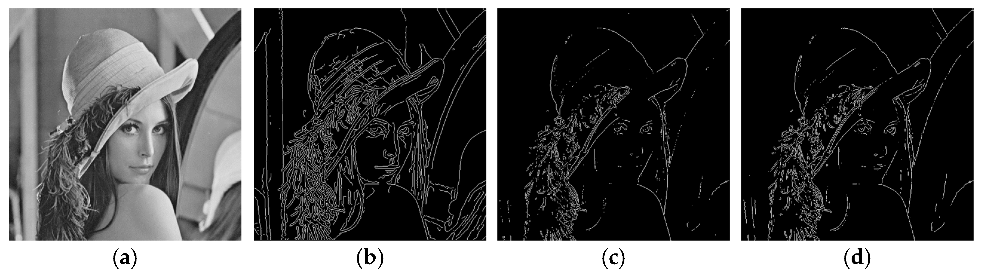
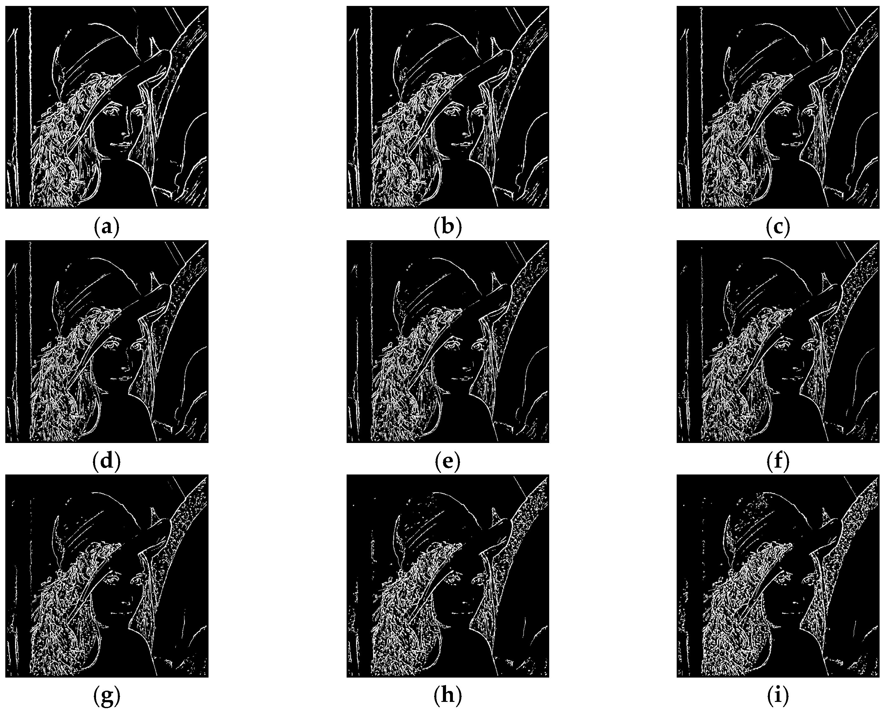
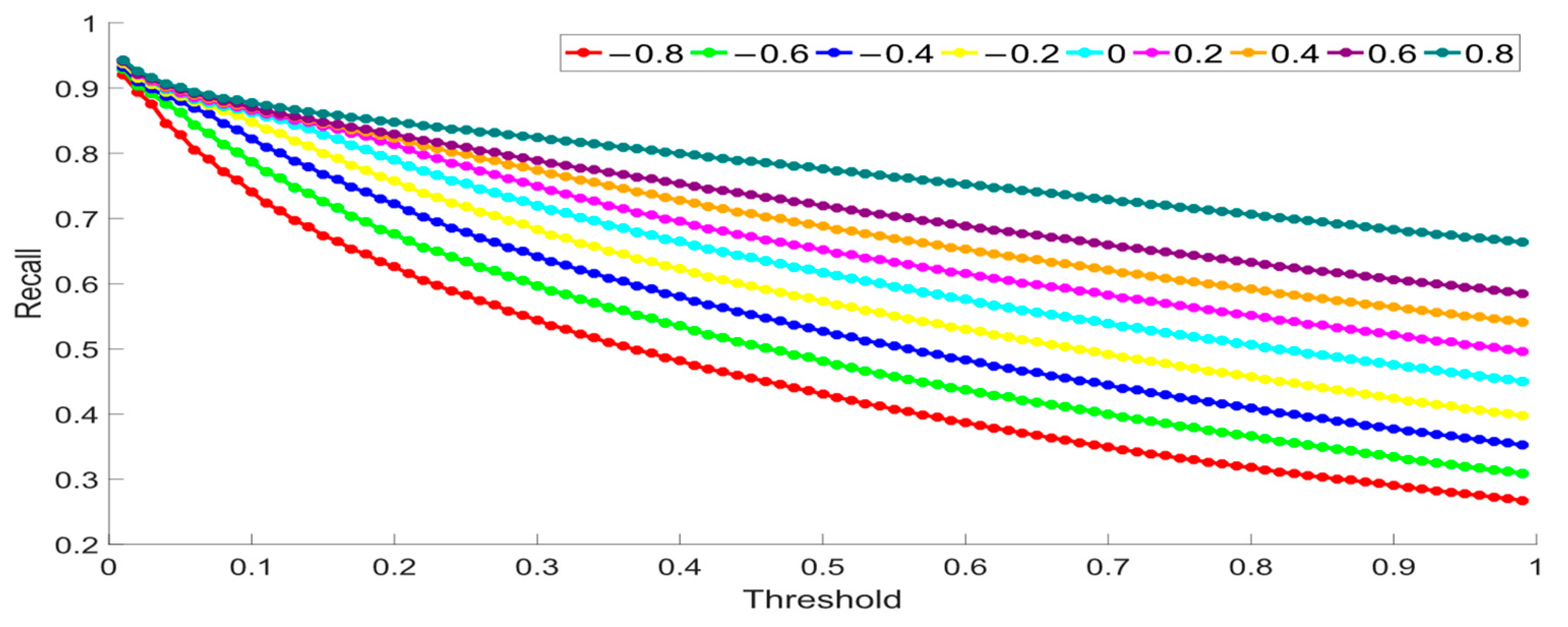
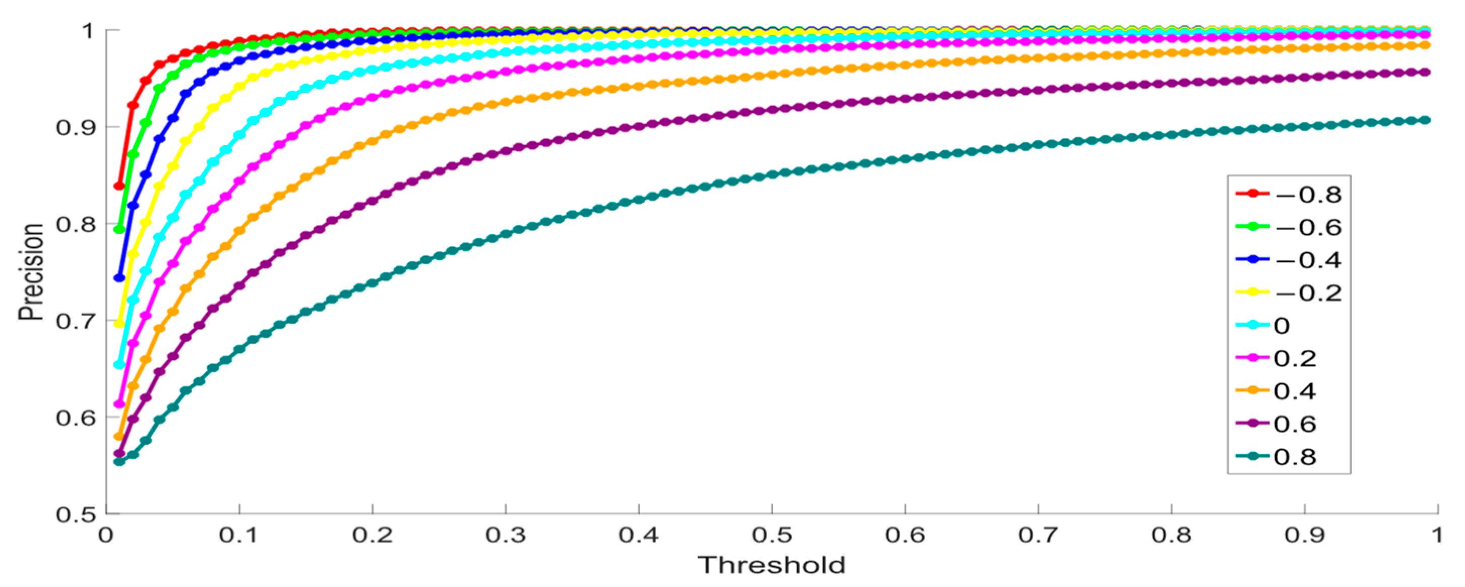
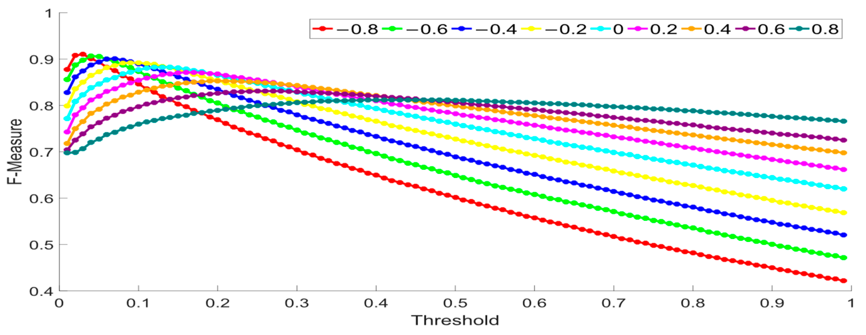
5.1. Effect of Fractional-Order Coefficients V in FACAFCV

In the first experiment, the fractional order ($-1<v<1$) of differential mask is adjusted to explore the effect on the edge detection performance. This is performed in order to gain insight into the sensitivity of the method to variations in fractional order, and to identify the optimal order for achieving the most accurate edge detection result. Moreover, by carefully varying the order of fractional differentiation and analyzing the corresponding edge detection outcomes, the experiment aims to shed light on the importance of fractional calculus in FACAFCV and its potential advantages over traditional integer-order methods.

Figure 2 shows the original image utilized for the experiment and the corresponding ground of truths obtained by the Canny, Roberts, and Sobel edge detection algorithms.

In Figure 3, the edge images for different $v$ corresponding to the optimal threshold (i.e., the threshold that maximizes F-measure) are depicted. By conducting a subjective analysis, it is found that as the fractional differential order increases, the contour of the texture region in the image becomes more pronounced while the edge information becomes less prominent. This can be attributed to the fact that fractional differential mask has the ability to amplify both the edges and texture regions of the image, with greater emphasis on texture regions as the order increases. Additionally, it is observed that as the fractional differential order decreases, the contour information of the texture region in the image gradually diminishes, while the detection of edge information becomes more prominent. This is due to the noise reduction capabilities of fractional differential mask, which allows for the preservation of edge and texture information in a balanced manner. To put it differently, if $v$ is larger than 0, the high-frequency details can be enhanced while still retaining the low-frequency information. Conversely, if $v$ is less than 0, the low-frequency information is enhanced while the high-frequency information is preserved. In the case where $v$ equals 0, FACAFCV becomes FACACV. These findings demonstrate the effectiveness of fractional differential operator in image processing.

Figure 4, Figure 5 and Figure 6 show the indicators obtained by varying the $v$ of FACAFCV. Each order is tested ten times. Firstly, an increase in the fractional differential order is associated with an increase in image recall. Secondly, a decrease in the fractional differential order leads to an increase in image precision. Thirdly, we observe that the F-measure gradually increases within the range of 0 to 0.5 about threshold, and then gradually decreases within the range of 0.5 to 1 about threshold. Each curve displays a peak value, representing the optimal F-measure. The corresponding threshold under the optimal F-measure is defined as the optimal threshold.

Table 2. The metrics correspond to the optimal F-measure of edge images obtained by FACAFCV with different fractional differential orders.

v	Threshold	Recall	Precision	F-Measure
−0.8	0.03	0.8761	0.9471	0.9102
−0.6	0.04	0.8733	0.9426	0.9066
−0.4	0.07	0.8612	0.9453	0.9013
−0.2	0.10	0.8513	0.9380	0.8925
0	0.13	0.8418	0.9280	0.8828
0.2	0.17	0.8330	0.9142	0.8717
0.4	0.20	0.8215	0.8884	0.8536
0.6	0.27	0.8011	0.8644	0.8315
0.8	0.44	0.7916	0.8355	0.8129

shows the relationship between the order of FACAFCV and indicators under the optimal threshold. With a decrease in the order of the fractional differential mask, there is less capacity to detect texture information. In general, the texture of the ground truths is constrained. Thus, it can be observed that a decrease in the order of fractional differential mask leads to an improvement in the edge detection indicators. Simultaneously, it is observable that the augmentation in the order leads to a corresponding decrease. This can be attributed to the fact that with an increase in the order of the fractional differential mask, the pertinent edge and texture information is suitably amplified, thus facilitating the extraction of more intricate details via the FACAFCV.

In conclusion, there are several key takeaways. Firstly, an increase in the order of fractional differential mask allows for detecting more texture information, which is advantageous for edge detection in blurred images. This is because fractional differential mask can amplify high-frequency information while preserving low-frequency information when $v>0$. Secondly, decreasing the order of fractional differential mask leads to the detection of less texture information while retaining most of the edge information. This is because fractional differential mask can amplify low-frequency information and retain high-frequency information when $v<0$. Thirdly, when $v$ of FACAFCV equals 0, the edge detection performance is inferior to the detection result when $v<0$. Therefore, it is possible to adjust the order of fractional differential mask adaptively to detect edge or texture information according to specific requirements.

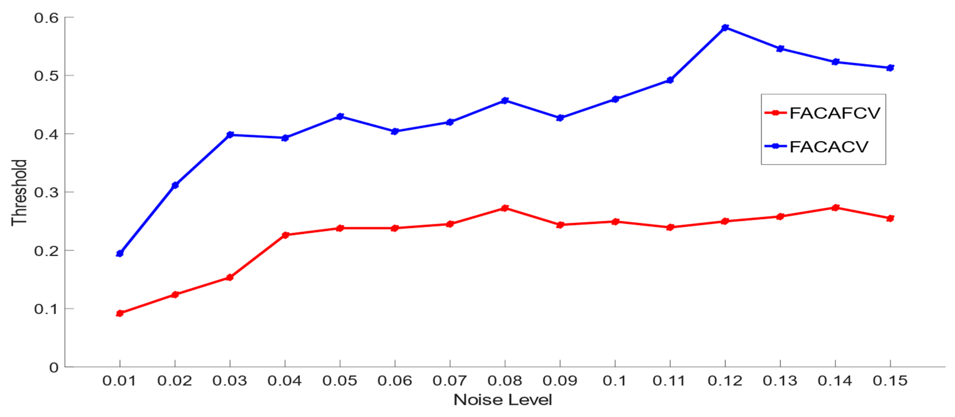
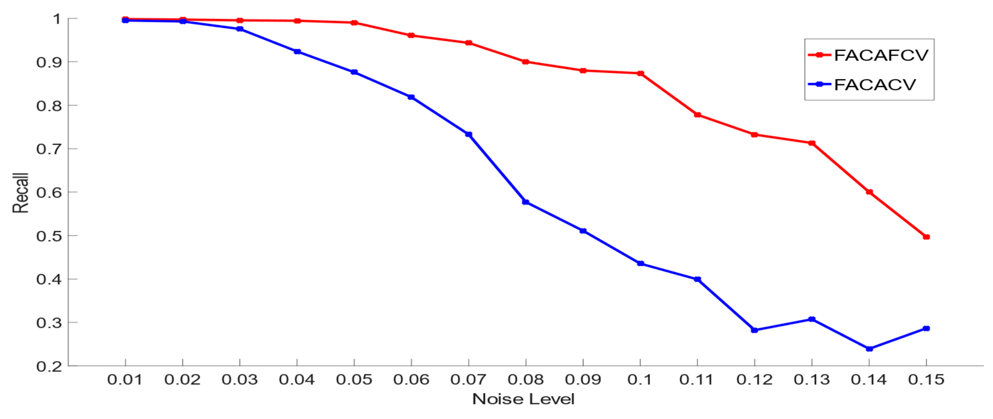
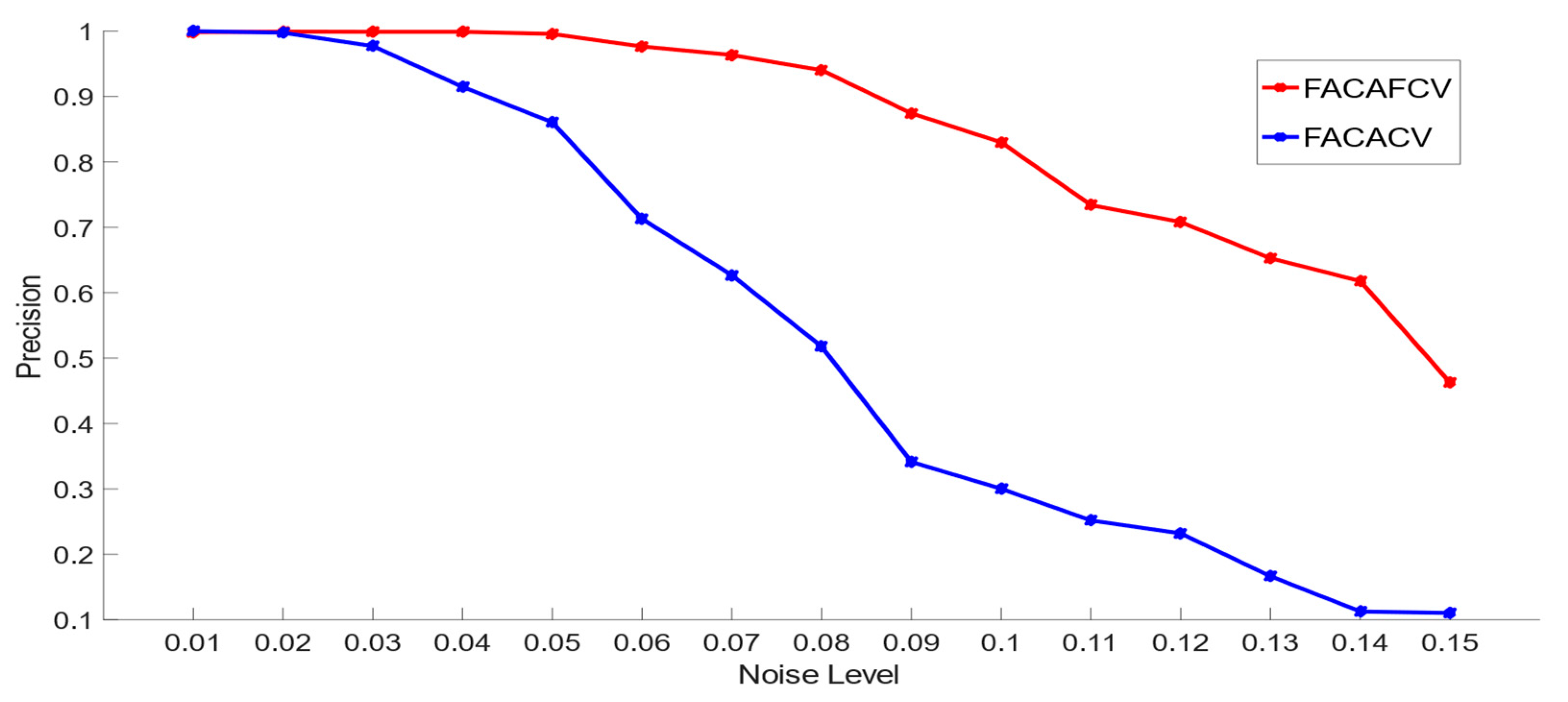
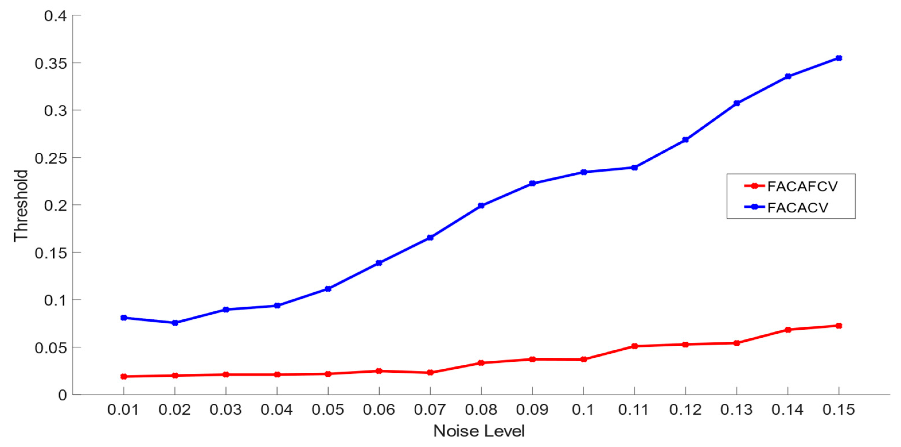
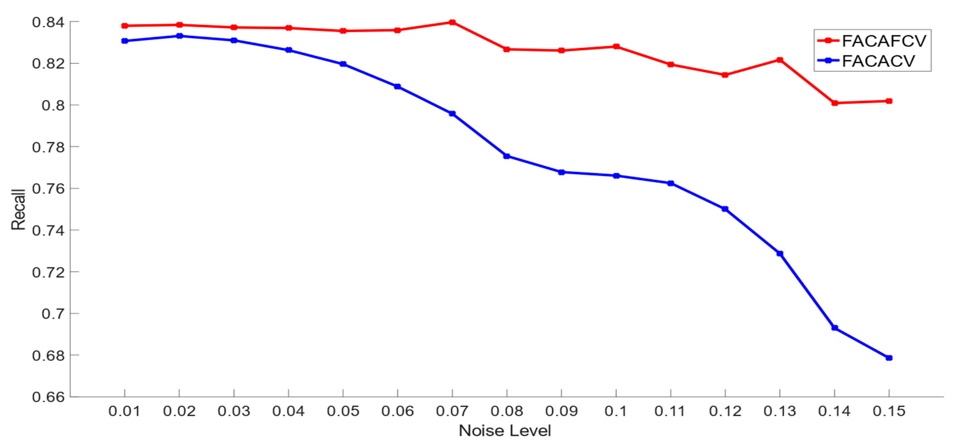
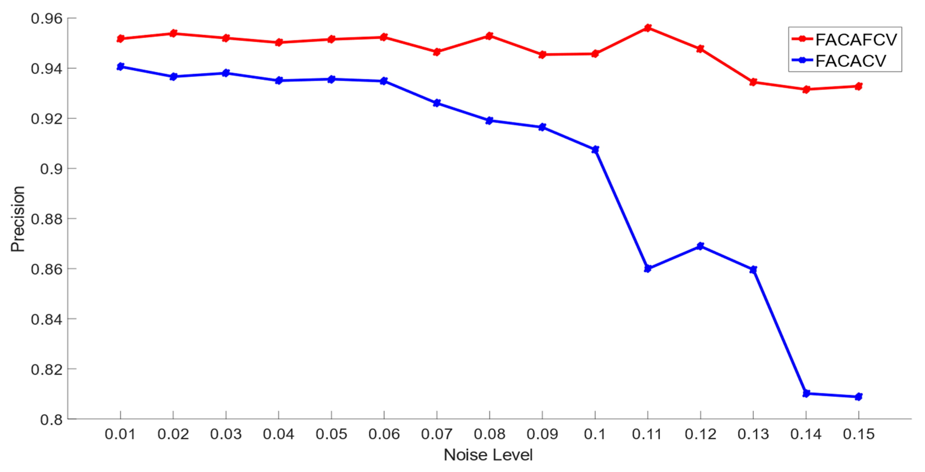
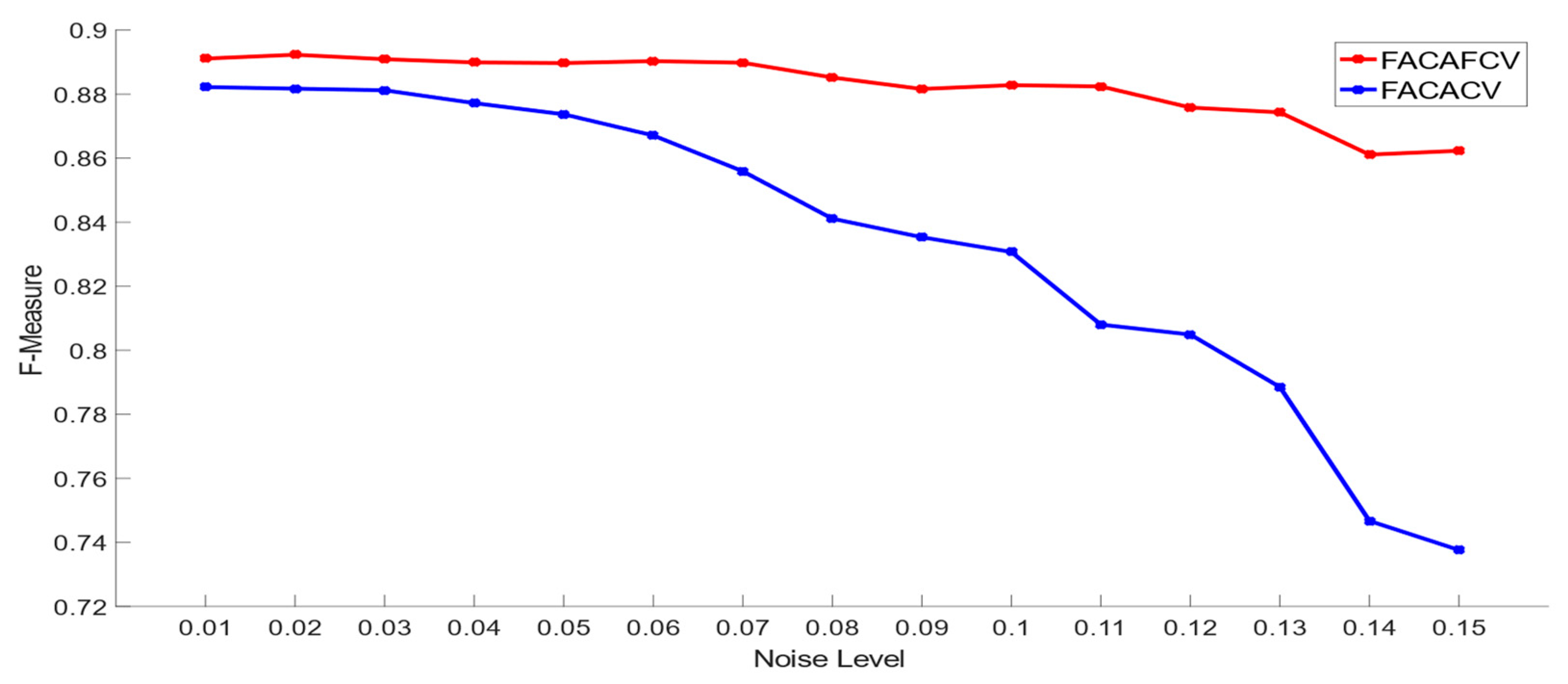
5.2. Comparison of FACAFCV and FACACV on Images with Multiplicative Noise

In the second experiment, the noise resistance of FACAFCV and FACACV is investigated. Firstly, we would like to express that the value of the parameter $v$ for FACAFCV in this experiment is −0.8 based on the results and analysis of the first experiment. In order to perform an unbiased and impartial analysis of FACAFCV and FACACV, we carry out experiments on both synthetic and real images. We then compare the results through observation and analysis.

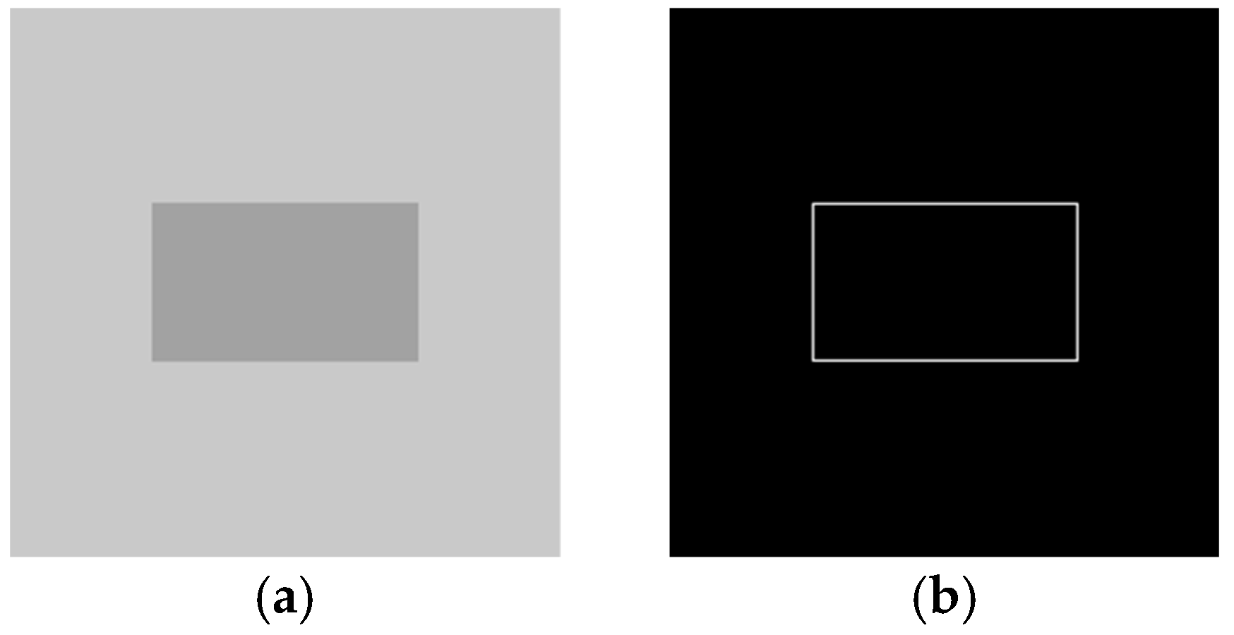
5.2.1. Synthetic Image

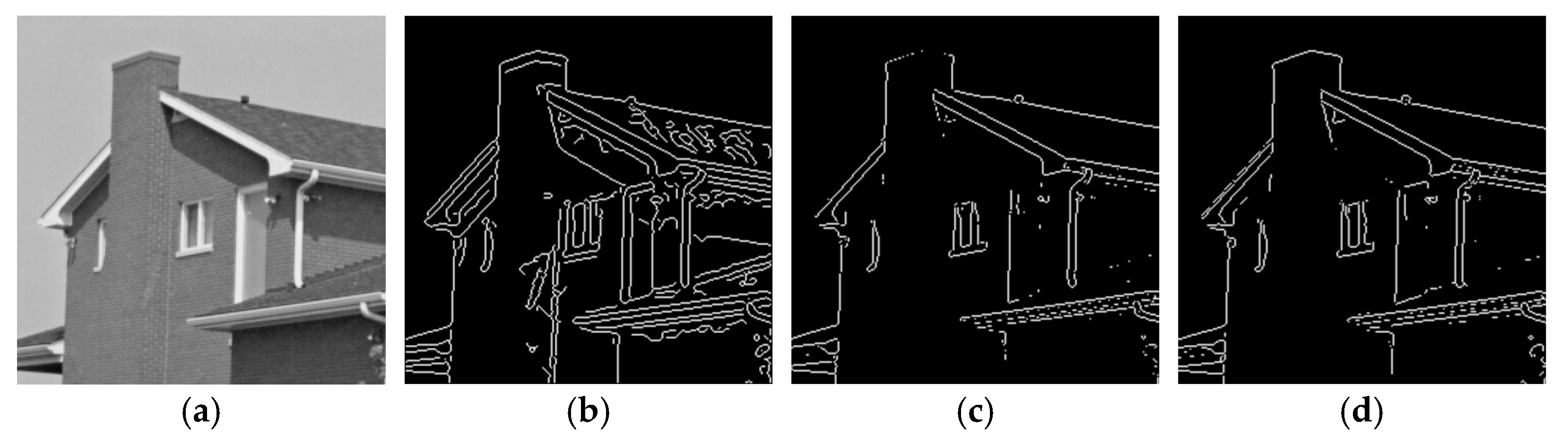
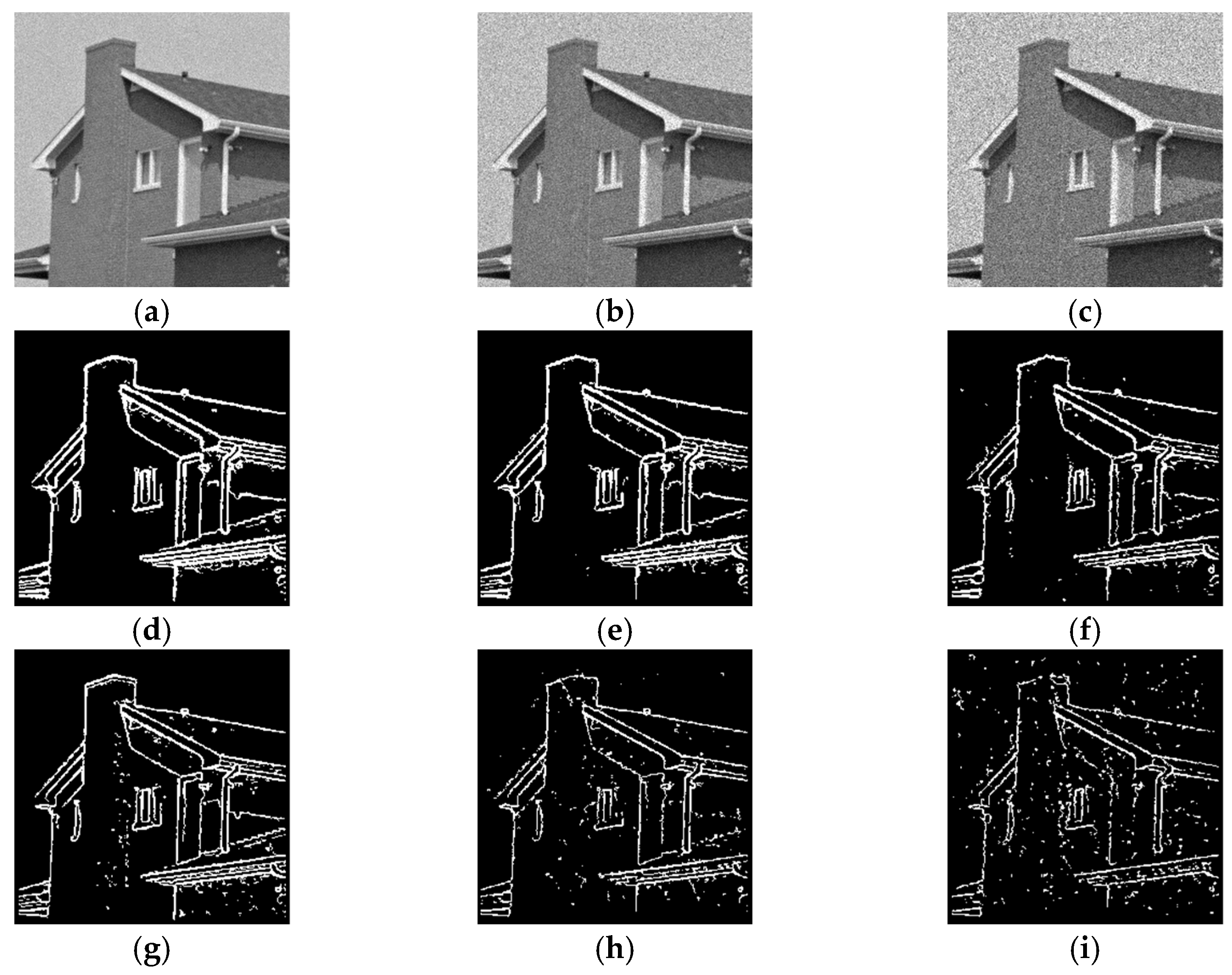
As can be seen in Figure 7, the left one is a synthetic image while the right one is an artificially marked ground truth.

In Figure 8, we present the results of processing three images with varying levels of noise, having standard deviations of 0.05, 0.1, and 0.15, respectively. A standard deviation of 0.05 indicates low level of noise, 0.1 represents medium level of noise, and 0.15 corresponds to high level of noise. As observed, both FACAFCV and FACACV exhibit good noise resistance capability when processing images with low and medium levels of noise. However, when dealing with a high level of noise, the performance of FACAFCV is significantly better than that of FACACV. Nevertheless, FACAFCV may still be affected to a certain extent.

Table 3. Metrics under optimal F-measure of synthetic images.

	Low Level of Noise		Medium Level of Noise		High Level of Noise
	FACAFCV	FACACV	FACAFCV	FACACV	FACAFCV	FACACV
Recall	0.9923	0.8776	0.9286	0.4923	0.5689	0.2857
Precision	1.0000	0.8982	0.8771	0.3333	0.5247	0.1532
F-Measure	0.9962	0.8877	0.9021	0.3975	0.5459	0.1995
Threshold	0.25	0.43	0.25	0.44	0.26	0.57

displays the indicators for the optimal F-measure of Figure 8. On the one hand, in a low level of noise, there is little difference between the recall, precision, and F-measure metrics. However, the threshold for FACAFCV is significantly lower than that for FACACV. On the other hand, when dealing with medium and high levels of noise, the recall, precision, and F-measure for FACAFCV are significantly higher than those for FACACV. Apparently, the rate of threshold adjustment for FACAFCV is lower than that for FACACV. It is apparent that FACAFCV demonstrates superior noise resistance in comparison to FACACV.

Figure 9, Figure 10, Figure 11 and Figure 12 represent the indicators obtained at different noise levels. Each noise level is tested twenty times. Our results show that the threshold of FACAFCV remains relatively stable across different noise levels. However, for FACACV, there is a clear upward trend in the threshold as the noise level increases. Moving on to recall, we observe that both FACAFCV and FACACV exhibit a decreasing trend as the noise level increases, but the curve of FACAFCV is consistently higher than that of FACACV. Similarly, in terms of precision, both FACAFCV and FACACV display a decreasing trend as the noise level increases, with the curve of FACAFCV consistently above that of FACACV. Meanwhile, with respect to F-measure, the FACAFCV curve is significantly higher and more stable than that of FACACV, indicating that FACACV exhibits some degree of noise resistance to multiplicative noise, but its noise resistance is significantly weaker than that of FACAFCV. Finally, it is demonstrated in synthetic images that FACAFCV outperforms FACACV in terms of noise resistance.

5.2.2. Real Image

To evaluate the noise resistance of FACAFCV and FACACV on real images, we conduct experiments following the same methodology as that of the synthetic image. Since there are different standards for ground of truth of real images, as can be seen from Figure 13, we use Canny, Roberts, and Sobel edge detection methods to extract edges and further thin them to obtain the final ground of truth for more objective analysis of the effects of FACAFCV and FACACV.

In Figure 14, we commence by utilizing images with three different levels of noise, having standard deviations of 0.05, 0.1, and 0.15, respectively. As observed, under low and medium levels of noise, the edge detection performance of FACAFCV is comparable to that of FACACV. However, compared to FACACV in high levels of noise, it is evident that the edge image produced by FACAFCV contains fewer significant noise points and has better image quality.

Table 4. Metrics under optimal F-measure of real images.

	Low Level of Noise		Medium Level of Noise		High Level of Noise
	FACAFCV	FACACV	FACAFCV	FACACV	FACAFCV	FACACV
Recall	0.8362	0.8278	0.8236	0.7587	0.7943	0.6799
Precision	0.9535	0.9260	0.9551	0.9138	0.9408	0.7886
F-Measure	0.8910	0.8741	0.8845	0.8291	0.8614	0.7302
Threshold	0.02	0.1	0.04	0.24	0.08	0.35

displays the indicators for the optimal F-measure of Figure 14. In low and medium levels of noise, there is little difference between the recall, precision, and F-measure metrics. The change in threshold for FACACV is more noticeable than for FACAFCV. However, when dealing with high levels of noise, the recall, precision, and F-measure for FACAFCV are higher than those for FACACV. Meanwhile, the change in FACAFCV is not significant. Furthermore, the rate of threshold adjustment for FACAFCV is lower than that of FACACV. It is evident that FACAFCV exhibits greater resistance to noise compared to FACACV.

Figure 15, Figure 16, Figure 17 and Figure 18 represent the indicators obtained at different noise levels. Initially, it is apparent that the threshold of FACAFCV exhibits a slight upward fluctuation as the noise level increases. However, as the noise level increases, the corresponding threshold of FACACV shows a clear upward trend. Secondly, concerning the recall, both FACAFCV and FACACV have a downward trend as the noise level increases, but FACAFCV consistently exceeds FACACV. Thirdly, in terms of precision, both FACAFCV and FACACV exhibit a declining trend as noise increases. Similarly, the FACAFCV curve lies above the FACACV and is more stable. Fourthly, when considering the F-measure, it is observed that the FACAFCV curve surpasses the FACACV curve by a considerable margin, indicating better performance. Moreover, the FACAFCV curve demonstrates greater stability. Finally, it is demonstrated in real images that FACAFCV outperforms FACACV in terms of noise resistance.

In conclusion, from the results obtained from our experiment involving both synthetic and real images, it is apparent that FACAFCV is superior to FACACV in the mitigation of multiplicative noise. The primary rationale behind this observation is that the fractional differential mask has the capability to preserve high-frequency details while also enhancing low-frequency features when $v$ is less than 0. This experiment also implies that FACACV possesses a certain degree of noise resistance, which is consistent with the stance proposed in the literature [28].

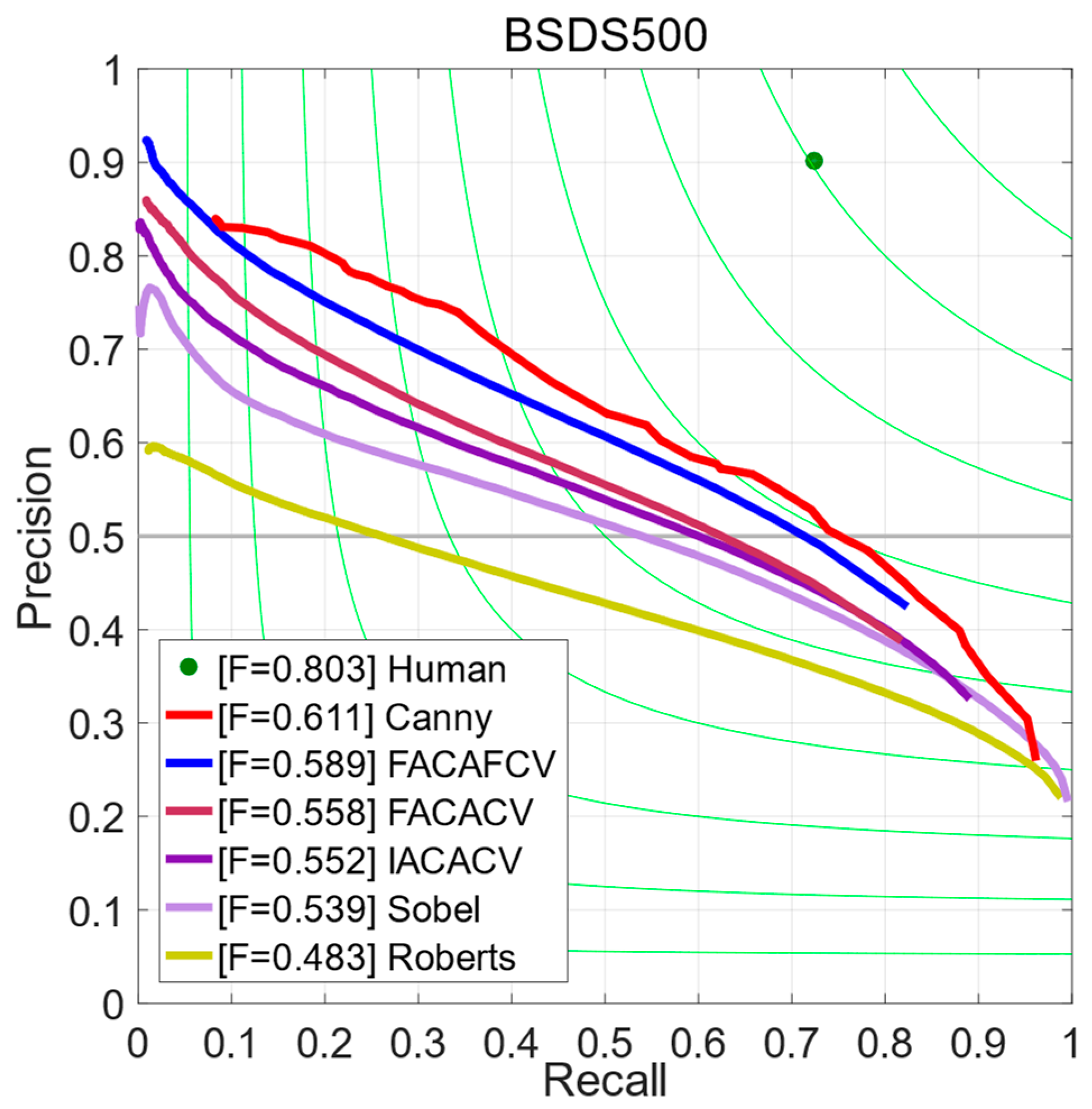
5.3. Test on BSDS500 Dataset

In the last experiment, a standard benchmark is conducted on a commonly utilized dataset. The DSDS500 dataset [44] has become widely accepted and utilized as a valuable tool for assessing the efficacy of edge detection algorithms [40,41,42]. The present experiment utilizes a set of fixed parameters, where the values of $v$ and $Q_p$ for FACAFCV are explicitly set to −0.9 and $⌊1.25Q_a⌋$, respectively, while the remaining parameters are held constant. All parameters for FACACV are identical to those of FACAFCV, except for variable $v$, which is absent in FACACV. The number of iterations, total quantity of ants, length of ant memory, and ant path length used in IACACV are in alignment with those utilized in FACAFCV. Meanwhile, the remaining parameters are consistent with those found in the relevant literature [28].

We compare the performance of our algorithm with that of several other algorithms in Figure 19, which displays the precision–recall (P-R) curves.

Table 5. The performance of different algorithms on BSDS500 dataset.

	ODS	OIS	Average Precision
Human	0.803	0.803	-
Canny	0.611	0.676	0.520
FACAFCV	0.589	0.608	0.533
FACACV	0.558	0.579	0.487
IACACV	0.552	0.571	0.497
Sobel	0.539	0.575	0.498
Roberts	0.483	0.513	0.413

presents the F-measure obtained using the ODS and OIS threshold division technologies [44].

Firstly, it is observed that FACACV demonstrates superior edge detection performance compared to IACACV [28]. The evidence once again substantiates the formidable advantages of fractional calculus. Secondly, it is worth noting that the edge detection performance of FACAFCV exhibits a noteworthy improvement over FACACV. Hence, the significance of the fractional differential mask becomes apparent. Finally, it is crucial to emphasize that the edge detection capability of FACAFCV is within the spectrum of the Sobel and Canny operators, with FACAFCV nearing the effectiveness of Canny. Furthermore, this research affirms the assertion present in earlier literature [25] that the edge detection ability of ant colony algorithm lies somewhere between the Canny and Sobel techniques.

6. Discussion and Future Directions

In this paper, due to the intrinsic characteristics of fractional calculus, such as long-term memory, non-locality, and weak singularity, we improve the edge detection capability of IACACV [28] by utilizing the theory of fractional calculus to produce FACAFCV for edge detection. In FACAFCV, we incorporate the fractional differential mask and CV during the initialization phase of heuristic function. Through numerous experiments, we first establish that varying the order of the fractional differential mask can detect distinct edge information. Then, we observe that FACAFCV displays superior noise immunity compared to FACACV when processing images with multiplicative noise. At last, we validate that FACACV surpasses IACACV in edge detection. Meanwhile, it was shown that the performance of FACAFCV is comparable to that of the Canny algorithm in detecting image edges without noise.

Despite its effectiveness, our algorithm is confronted with several limitations. Firstly, since images with different content exhibit diverse edge or texture information, FACAFCV requires the establishment of specific parameters for each image, thereby reducing generalizability of the algorithm. Therefore, an important area is adaptive parameter adjustment. Secondly, the number of ants utilized in the algorithm varies depending on the image size. Larger images necessitate a greater number of ants, resulting in more increased computational complexity and time consumption. Exploring the use of GPU-based parallel computing to accelerate the algorithm holds promise for future investigations. Thirdly, FACAFCV restricts the movement of ants to the 8-connectivity neighborhood of the current pixel, potentially leading to stagnation due to limited pixel selection. To address this issue, we have implemented preventive strategies. Meanwhile, expanding the crawling range or modifying the crawling mode of ants are potential directions for future work. Finally, Ant colony algorithm is merely one type of metaheuristic algorithm. Exploring the application of alternative metaheuristic algorithms to image processing is an essential avenue for future research.

Robust noise resistance and reliable recognition ability are demonstrated by our algorithm in detecting edges on images corrupted by multiplicative noise. This type of noise presents a common challenge in the accurate detection of edges, especially in ultrasound images. Consequently, our method provides a viable solution for image segmentation in medical ultrasound images and holds potential for future applications in non-destructive ultrasonic testing of objects.

Based on the above discussion and analysis, we have proposed a robust edge detection technique.

References

1. Chen, J.L.; Huang, C.H.; Du, Y.C.; Lin, C.H. Combining fractional-order edge detection and chaos synchronisation classifier for fingerprint identification. IET Image Process. 2014, 8, 354–362. [Google Scholar] [CrossRef]
2. Winarno, E.; Hadikurniawati, W.; Wibisono, S.; Septiarini, A. Edge Detection and Grey Level Co-Occurrence Matrix (GLCM) Algorithms for Fingerprint Identification. In Proceedings of the 2021 2nd International Conference on Innovative and Creative Information Technology (ICITech), Salatiga, Indonesia, 23–25 September 2021; pp. 30–34. [Google Scholar]
3. Anusha, K.; Siva Kumar, P. Fingerprint Image Enhancement for Crime Detection Using Deep Learning. In Proceedings of the International Conference on Cognitive and Intelligent Computing: ICCIC 2021, Hyderabad, India, 11–12 December 2021; Volume 2, pp. 257–268. [Google Scholar]
4. Chen, X.; Cheng, W. Facial expression recognition based on edge detection. Int. J. Comput. Sci. Eng. Surv. 2015, 6, 1. [Google Scholar] [CrossRef]
5. Zhao-Yi, P.; Yan-Hui, Z.; Yu, Z. Real-time facial expression recognition based on adaptive canny operator edge detection. In Proceedings of the 2010 Second International Conference on MultiMedia and Information Technology, Kaifeng, China, 24–25 April 2010; pp. 154–157. [Google Scholar]
6. Kakran, A.; Chaudhary, H.; Kumar, P.; Sharma, A.; Singh, H. Identification and Recognition of face and number Plate for Autonomous and Secure Car Parking. In Proceedings of the 2023 International Conference on Power, Instrumentation, Energy and Control (PIECON), Aligarh, India, 10–12 February 2023; pp. 1–6. [Google Scholar]
7. Al-Amri, S.S.; Kalyankar, N.; Khamitkar, S. Image segmentation by using edge detection. Int. J. Comput. Sci. Eng. 2010, 2, 804–807. [Google Scholar]
8. Arbeláez, P.; Pont-Tuset, J.; Barron, J.T.; Marques, F.; Malik, J. Multiscale combinatorial grouping. In Proceedings of the Proceedings of the IEEE Conference on Computer Vision and Pattern Recognition, Columbus, OH, USA, 23–28 June 2014; pp. 328–335. [Google Scholar]
9. Singh, K.K.; Singh, A. A study of image segmentation algorithms for different types of images. Int. J. Comput. Sci. Issues IJCSI 2010, 7, 414. [Google Scholar]
10. Tchinda, B.S.; Tchiotsop, D.; Noubom, M.; Louis-Dorr, V.; Wolf, D. Retinal blood vessels segmentation using classical edge detection filters and the neural network. Inform. Med. Unlocked 2021, 23, 100521. [Google Scholar] [CrossRef]
11. Sobel, I.E. Camera Models and Machine Perception; Stanford University: Stanford, CA, USA, 1970. [Google Scholar]
12. Prewitt, J.M. Object enhancement and extraction. Pict. Process. Psychopictorics 1970, 10, 15–19. [Google Scholar]
13. Roberts, L.G. Machine Perception of Three-Dimensional Solids; Massachusetts Institute of Technology: Cambridge, MA, USA, 1963. [Google Scholar]
14. Marr, D.; Hildreth, E. Theory of edge detection. Proc. R. Soc. Lond. Ser. B Biol. Sci. 1980, 207, 187–217. [Google Scholar]
15. Canny, J. A computational approach to edge detection. IEEE Trans. Pattern Anal. Mach. Intell. 1986, 8, 679–698. [Google Scholar] [CrossRef]
16. Dorigo, M.; Birattari, M.; Stutzle, T. Ant colony optimization. IEEE Comput. Intell. Mag. 2006, 1, 28–39. [Google Scholar] [CrossRef]
17. Dorigo, M.; Maniezzo, V.; Colorni, A. Ant system: Optimization by a colony of cooperating agents. IEEE Trans. Syst. Man Cybern. Part B Cybern. 1996, 26, 29–41. [Google Scholar] [CrossRef]
18. Dorigo, M.; Gambardella, L.M. Ant colony system: A cooperative learning approach to the traveling salesman problem. IEEE Trans. Evol. Comput. 1997, 1, 53–66. [Google Scholar] [CrossRef]
19. Stützle, T.; Hoos, H.H. MAX–MIN ant system. Future Gener. Comput. Syst. 2000, 16, 889–914. [Google Scholar] [CrossRef]
20. Yi-Fei, P.; Siarry, P.; Wu-Yang, Z.; Jian, W.; Zhang, N. Fractional-order ant colony algorithm: A fractional long term memory based cooperative learning approach. Swarm Evol. Comput. 2022, 69, 101014. [Google Scholar]
21. Gong, X.; Rong, Z.; Wang, J.; Zhang, K.; Yang, S. A hybrid algorithm based on state-adaptive slime mold model and fractional-order ant system for the travelling salesman problem. Complex Intell. Syst. 2022, 1–20. [Google Scholar] [CrossRef]
22. Zhu, W.; Pu, Y. A Study of Fractional-Order Memristive Ant Colony Algorithm: Take Fracmemristor into Swarm Intelligent Algorithm. Fractal Fract. 2023, 7, 211. [Google Scholar] [CrossRef]
23. Nezamabadi-Pour, H.; Saryazdi, S.; Rashedi, E. Edge detection using ant algorithms. Soft Comput. 2006, 10, 623–628. [Google Scholar] [CrossRef]
24. Tian, J.; Yu, W.; Xie, S. An ant colony optimization algorithm for image edge detection. In Proceedings of the 2008 IEEE congress on evolutionary computation (IEEE world congress on computational intelligence), Hong Kong, China, 1–6 June 2008; pp. 751–756. [Google Scholar]
25. Etemad, S.A.; White, T. An ant-inspired algorithm for detection of image edge features. Appl. Soft Comput. 2011, 11, 4883–4893. [Google Scholar] [CrossRef]
26. Liu, X.; Fang, S. A convenient and robust edge detection method based on ant colony optimization. Opt. Commun. 2015, 353, 147–157. [Google Scholar] [CrossRef]
27. Martínez, C.A.; Buemi, M.E. Hybrid ACO algorithm for edge detection. Evol. Syst. 2021, 12, 849–860. [Google Scholar] [CrossRef]
28. Baltierra, S.; Valdebenito, J.; Mora, M. A proposal of edge detection in images with multiplicative noise using the Ant Colony System algorithm. Eng. Appl. Artif. Intell. 2022, 110, 104715. [Google Scholar] [CrossRef]
29. Oldham, K.; Spanier, J. The Fractional Calculus Theory and Applications of Differentiation and Integration to Arbitrary Order; Elsevier: Amsterdam, The Netherlands, 1974. [Google Scholar]
30. He, N.; Wang, J.-B.; Zhang, L.-L.; Lu, K. An improved fractional-order differentiation model for image denoising. Signal Process. 2015, 112, 180–188. [Google Scholar] [CrossRef]
31. Pu, Y.-F. Fractional-order euler-Lagrange equation for fractional-order variational method: A necessary condition for fractional-order fixed boundary optimization problems in signal processing and image processing. IEEE Access 2016, 4, 10110–10135. [Google Scholar] [CrossRef]
32. Li, C.; He, C. Fractional-order diffusion coupled with integer-order diffusion for multiplicative noise removal. Comput. Math. Appl. 2023, 136, 34–43. [Google Scholar] [CrossRef]
33. Kommula, B.N.; Kota, V.R. Design of MFA-PSO based fractional order PID controller for effective torque controlled BLDC motor. Sustain. Energy Technol. Assess. 2022, 49, 101644. [Google Scholar]
34. Padula, F.; Visioli, A. Tuning rules for optimal PID and fractional-order PID controllers. J. Process Control 2011, 21, 69–81. [Google Scholar] [CrossRef]
35. Li, X.; Mou, J.; Banerjee, S.; Wang, Z.; Cao, Y. Design and DSP implementation of a fractional-order detuned laser hyperchaotic circuit with applications in image encryption. Chaos Solitons Fractals 2022, 159, 112133. [Google Scholar] [CrossRef]
36. Xu, J.; Mou, J.; Liu, J.; Hao, J. The image compression–encryption algorithm based on the compression sensing and fractional-order chaotic system. Vis. Comput. 2022, 38, 1509–1526. [Google Scholar] [CrossRef]
37. Pu, Y.-F.; Zhou, J.-L.; Yuan, X. Fractional differential mask: A fractional differential-based approach for multiscale texture enhancement. IEEE Trans. Image Process. 2009, 19, 491–511. [Google Scholar]
38. Samko, S.G.; Kilbas, A.A.; Marichev, O.I. Fractional Integrals and Derivatives; Gordon and Breach Science Publishers: Yverdon Yverdon-les-Bains, Switzerland, 1993; Volume 1. [Google Scholar]
39. Podlubny, I. An introduction to fractional derivatives, fractional differential equations, to methods of their solution and some of their applications. Math. Sci. Eng 1999, 198, 340. [Google Scholar]
40. Su, Z.; Liu, W.; Yu, Z.; Hu, D.; Liao, Q.; Tian, Q.; Pietikäinen, M.; Liu, L. Pixel difference networks for efficient edge detection. In Proceedings of the IEEE/CVF International Conference on Computer Vision, Montreal, BC, Canada, 11–17 October 2021; pp. 5117–5127. [Google Scholar]
41. Xie, S.; Tu, Z. Holistically-nested edge detection. In Proceedings of the IEEE International Conference on Computer Vision, Santiago, Chile, 7–13 December 2015; pp. 1395–1403. [Google Scholar]
42. Yang, J.; Price, B.; Cohen, S.; Lee, H.; Yang, M.-H. Object contour detection with a fully convolutional encoder-decoder network. In Proceedings of the IEEE Conference on Computer Vision and Pattern Recognition, Las Vegas, NV, USA, 26 June–1 July 2016; pp. 193–202. [Google Scholar]
43. Lam, L.; Lee, S.-W.; Suen, C.Y. Thinning methodologies-a comprehensive survey. IEEE Trans. Pattern Anal. Mach. Intell. 1992, 14, 869–885. [Google Scholar] [CrossRef]
44. Arbelaez, P.; Maire, M.; Fowlkes, C.; Malik, J. Contour detection and hierarchical image segmentation. IEEE Trans. Pattern Anal. Mach. Intell. 2010, 33, 898–916. [Google Scholar] [CrossRef]
45. Achim, A.; Bezerianos, A.; Tsakalides, P. Novel Bayesian multiscale method for speckle removal in medical ultrasound images. IEEE Trans. Med. Imaging 2001, 20, 772–783. [Google Scholar] [CrossRef]
46. Krissian, K.; Westin, C.-F.; Kikinis, R.; Vosburgh, K.G. Oriented speckle reducing anisotropic diffusion. IEEE Trans. Image Process. 2007, 16, 1412–1424. [Google Scholar] [CrossRef]
47. Mora, M.; Córdova-Lepe, F.; Del-Valle, R. A non-Newtonian gradient for contour detection in images with multiplicative noise. Pattern Recognit. Lett. 2012, 33, 1245–1256. [Google Scholar] [CrossRef]
Figure 1. 8-connectivity neighborhood.
Fractalfract 07 00420 g001
Figure 2. Original image and ground truths: (a) Original image; (b) Ground truth obtained by Canny; (c) Ground truth obtained by Roberts; (d) Ground truth obtained by Sobel.
Fractalfract 07 00420 g002
Figure 3. The impact of fractional-order coefficients v in FACAFCV: (a) −0.8; (b) −0.6; (c) −0.4; (d) −0.2; (e) 0; (f) 0.2; (g) 0.4; (h) 0.6; (i) 0.8.
Fractalfract 07 00420 g003
Figure 4. Average recall curves of edge images obtained by FACAFCV with different fractional differential orders.
Fractalfract 07 00420 g004
Figure 5. Average precision curves of edge images obtained by FACAFCV with different fractional differential orders.
Fractalfract 07 00420 g005
Figure 6. Average F-measure curves of edge images obtained by FACAFCV with different fractional differential orders.
Fractalfract 07 00420 g006
Figure 7. Synthetic image and ground truth: (a) Original image; (b) Manually labeled ground truth.
Fractalfract 07 00420 g007
Figure 8. Synthetic image: (a) Low level of noise; (b) Medium level of noise; (c) High level of noise; (d) Low level of noise of FACAFCV; (e) Medium level of noise of FACAFCV; (f) High level of noise of FACAFCV; (g) Low level of noise of FACACV; (h) Medium level of noise of FACACV; (i) High level of noise of FACACV.
Fractalfract 07 00420 g008
Figure 9. Average threshold curves of edge images obtained by FACAFCV and FACACV on synthetic images with different noise levels.
Fractalfract 07 00420 g009
Figure 10. Average recall curves of edge images obtained by FACAFCV and FACACV on synthetic images with different noise levels.
Fractalfract 07 00420 g010
Figure 11. Average precision curves of edge images obtained by FACAFCV and FACACV on synthetic images with different noise levels.
Fractalfract 07 00420 g011
Figure 12. Average F-measure curves of edge images obtained by FACAFCV and FACACV on synthetic images with different noise levels.
Fractalfract 07 00420 g012
Figure 13. Real image and ground truths: (a) Original image; (b) Ground truth obtained by Canny; (c) Ground truth obtained by Roberts; (d) Ground truth obtained by Sobel.
Fractalfract 07 00420 g013
Figure 14. Real image: (a) Low level of noise; (b) Medium level of noise; (c) High level of noise; (d) Low level of noise of FACAFCV; (e) Medium level of noise of FACAFCV; (f) High level of noise of FACAFCV; (g) Low level of noise of FACACV; (h) Medium level of noise of FACACV; (i) High level of noise of FACACV.
Fractalfract 07 00420 g014
Figure 15. Average threshold curves of edge images obtained by FACAFCV and FACACV on real images with different noise levels.
Fractalfract 07 00420 g015
Figure 16. Average recall curves of edge images obtained by FACAFCV and FACACV on real images with different noise levels.
Fractalfract 07 00420 g016
Figure 17. Average precision curves of edge images obtained by FACAFCV and FACACV on real images with different noise levels.
Fractalfract 07 00420 g017
Figure 18. Average F-measure curves of edge images obtained by FACAFCV and FACACV on real images with different noise levels.
Fractalfract 07 00420 g018
Figure 19. The precision–recall (P-R) curves of different algorithms on BSDS500 dataset.
Fractalfract 07 00420 g019