Article

Fractional-Order Model-Free Predictive Control for Voltage Source Inverters

1
Electrical Engineering Department, Faculty of Engineering, University of Tabuk, Tabuk 47913, Saudi Arabia
2
Renewable Energy and Energy Efficiency Centre (REEEC), University of Tabuk, Tabuk 47913, Saudi Arabia
3
Electrical Engineering Department, Faculty of Engineering, Aswan University, Aswan 81542, Egypt
4
Sensor Networks and Cellular Systems (SNCS) Research Center, University of Tabuk, Tabuk 71491, Saudi Arabia
5
College of Engineering, Effat University, Jeddah 21478, Saudi Arabia
*
Authors to whom correspondence should be addressed.
Fractal Fract. 2023, 7(6), 433; https://doi.org/10.3390/fractalfract7060433
Submission received: 7 April 2023 / Revised: 20 May 2023 / Accepted: 25 May 2023 / Published: 27 May 2023

Abstract

:
Currently, a two-level voltage source inverter (2L-VSI) is regarded as the cornerstone of modern industrial applications. However, the control of VSIs is a challenging task due to their nonlinear and time-varying nature. This paper proposes employing the fractional-order controller (FOC) to improve the performance of model-free predictive control (MFPC) of the 2L-VSI voltage control in uninterruptible power supply (UPS) applications. In the conventional MFPC based on the ultra-local model (ULM), the unknown variable that includes all the system disturbances is estimated using algebraic identification, which is insufficient to improve the prediction accuracy in the predictive control. The proposed FO-MFPC uses fractional-order proportional-integral control (FOPI) to estimate the unknown function associated with the MFPC. To get the best performance from the FOPI, its parameters are optimally designed using the grey wolf optimization (GWO) approach. The number of iterations of the GWO is 100, while the grey wolf’s number is 20. The proposed GWO algorithm achieves a small fitness function value of approximately 0.156. In addition, the GWO algorithm nearly finds the optimal parameters after 80 iterations for the defined objective function. The performance of the proposed FO-MFPC controller is compared to that of conventional MFPC for the three loading cases and conditions. Using MATLAB simulations, the simulation results indicated the superiority of the proposed FO-MFPC controller over the conventional MFPC in steady state and transient responses. Moreover, the total harmonic distortion (THD) of the output voltage at different sampling times proves the excellent quality of the output voltage with the proposed FO-MFPC controller over the conventional MFPC controller. The results confirm the robustness of the two control systems against parameter mismatches. Additionally, using the TMS320F28379D kit, the experimental verification of the proposed FO-MFPC control strategy is implemented for 2L-VSI on the basis of the Hardware-in-the-Loop (HIL) simulator, demonstrating the applicability and effective performance of our proposed control strategy under realistic circumstances.

1. Introduction

Voltage source inverters (VSIs) are widely used in power electronic systems for applications, such as renewable energy systems, electric vehicles, and industrial drives [1,2,3]. However, controlling VSIs is challenging due to their nonlinear and time-varying nature [4,5,6,7]. Additionally, the reliability of the VSI is at risk as a result of the likelihood of a short-circuit occurring between the two switches located on the same leg. This potential problem could compromise the overall functioning and performance of the VS. Conventional VSIs, also called two-level inverters, are limited to only two output levels and require particular features to achieve high-quality output [8]. Although it has the merit of simplicity, two-level VSI has the drawbacks of high switching frequency, high switching stresses, power losses, and electromagnetic interference. There is now multilevel architecture, which overcomes the disadvantages of conventional inverters. The famous multilevel VSI topologies are the cascaded [9], flying capacitor [10], and neutral point clamped multilevel inverters [11]. The number of output voltage levels is the primary distinction between multilevel inverters and conventional VSI topologies. Many control techniques have been implemented in the literature, such as internal model controllers, hysteresis controllers, proportional-resonant controllers, proportional-integral controllers, and deadbeat controllers [12]. The finite control set-model predictive control (FCS-MPC) has several advantages over other control methods: its simplicity, ability to handle nonlinearity, and fast response during transients [13,14,15]. However, the FCS-MPC’s performance depends on the system model’s accuracy [16]. In recent years, model-free predictive control (MFPC) has emerged as a promising approach to VSI control. It has been widely used in many applications, such as energy management and intelligent transportation [17].
MFPC is a control strategy that uses historical data to predict the future behavior of a system, then uses this information to determine the control action. Unlike traditional model-based control methods, MFPC does not require a detailed system dynamics model. This makes it suitable for complex or uncertain dynamic systems, such as VSIs [18,19,20,21]. One of the main advantages of MFPC for VSI control is its ability to handle nonlinear and time-varying system dynamics. MFPC can handle these dynamics using a prediction model updated with real-time data. This allows the control algorithm to adapt to changes in the system dynamics, resulting in improved control performance. Another advantage of MFPC for VSI control is its ability to handle constraints. MFPC can consider constraints, such as voltage, current, and power limits, and use this information to determine the optimal control action. This improves the robustness of the control algorithm and reduces the risk of system failures.
Several studies have been conducted on the application of MFPC to VSI control. For example, a study has proposed an MPC-based control strategy for a VSI in a wind energy system [22]. The authors used a prediction model based on historical data to predict the wind speed and power output of the wind turbine. The control algorithm then used this information to determine the optimal VSI control action. The authors found that the MPC-based control strategy improved the performance of the VSI compared to a traditional model-based control strategy. Another study [23] proposed a neural network-based MFPC controller for the rigorous performance of the power converters. The authors utilized a new framework named the state-space neural network to implement the MFPC controller for the 3-Φ VSI converters. Though the proposed system was robust, the architecture of the neural network structure is unavoidably affected by the nonlinearities in the system. An innovative MFPC controller has been introduced [24] for three-level grid-connected inverters. The proposal was amazing; however, the system was complex. In [25], a modified MFPC technique has been introduced for pulse width modulation (PWM) converters. To achieve excellent performance, the technique has utilized two successive current samples. A new MFPC strategy has been implemented for the DC choppers; however, it does not apply to 3-Φ converters [26]. The observer has been built to enhance the performance of the MPC against parameter uncertainty.
Fractional-order control (FOC) is a relatively new control technique that has been applied to various systems, including voltage source inverters (VSIs) [27,28,29]. FOC is an extension of traditional integer order control and offers several advantages over conventional control techniques, such as improved performance, better robustness, and increased flexibility. Additionally, FOC can improve the VSI output’s power quality, reducing harmonic and total harmonic distortion (THD). It can control current and voltage in a VSI, whereas traditional integer order control is typically used to control only one of these variables. Despite these advantages, there are also some disadvantages to FOC. The main disadvantages are the complexity, difficulty of implementation, and computationally intensive nature.
Several studies have been conducted on applying FOC to VSIs, and the results have been promising. A controller that utilizes FOC and repetition control principles has been proposed to eliminate harmonics and steady-state errors in power converters [30]. In [31], a robust FOC for VSIs was utilized in microgrid applications. Although the performance of the control system has improved, the presence of load variations has affected its robustness.
Despite the significant reduction in VSI-dependent parameters, finding the appropriate function in the MFPC’s input-output relationship still poses a challenge. This paper introduces using FOC and MFPC controllers with 2L-VSI for UPS applications. Combining these controllers allows for more accurate and efficient operation of the UPS system. The basic goal of the control system is to keep the output voltage on the load terminals sinusoidal with low harmonic distortions. The fractional-order proportional integral (FOPI) is a numerical method used to calculate the unknown function in the MFPC, representing the total disturbances of the system. Consequently, the MFPC can predict the output voltage at different voltage vectors and choose the one that results in the best performance. Moreover, the FOPI gains are optimally selected using the GWO approach. The main contributions of this study can be summarized as follows:
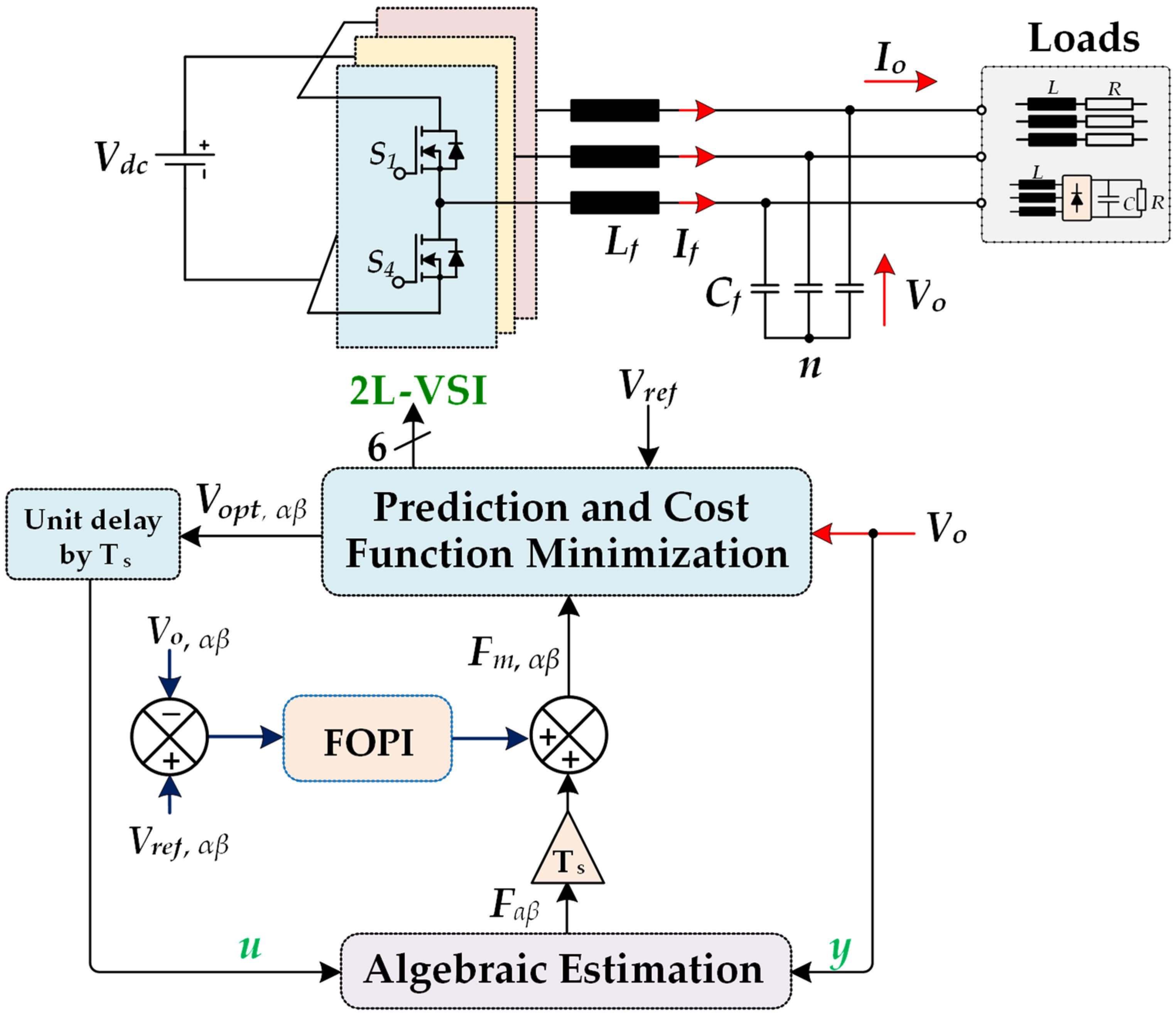
  • The FOPI controller and the MFPC controllers have been integrated to improve the performance of the 2L-VSI. This has been carried out by accurately estimating the unknown function of the MFPC for the voltage control of the 2L-VSI.
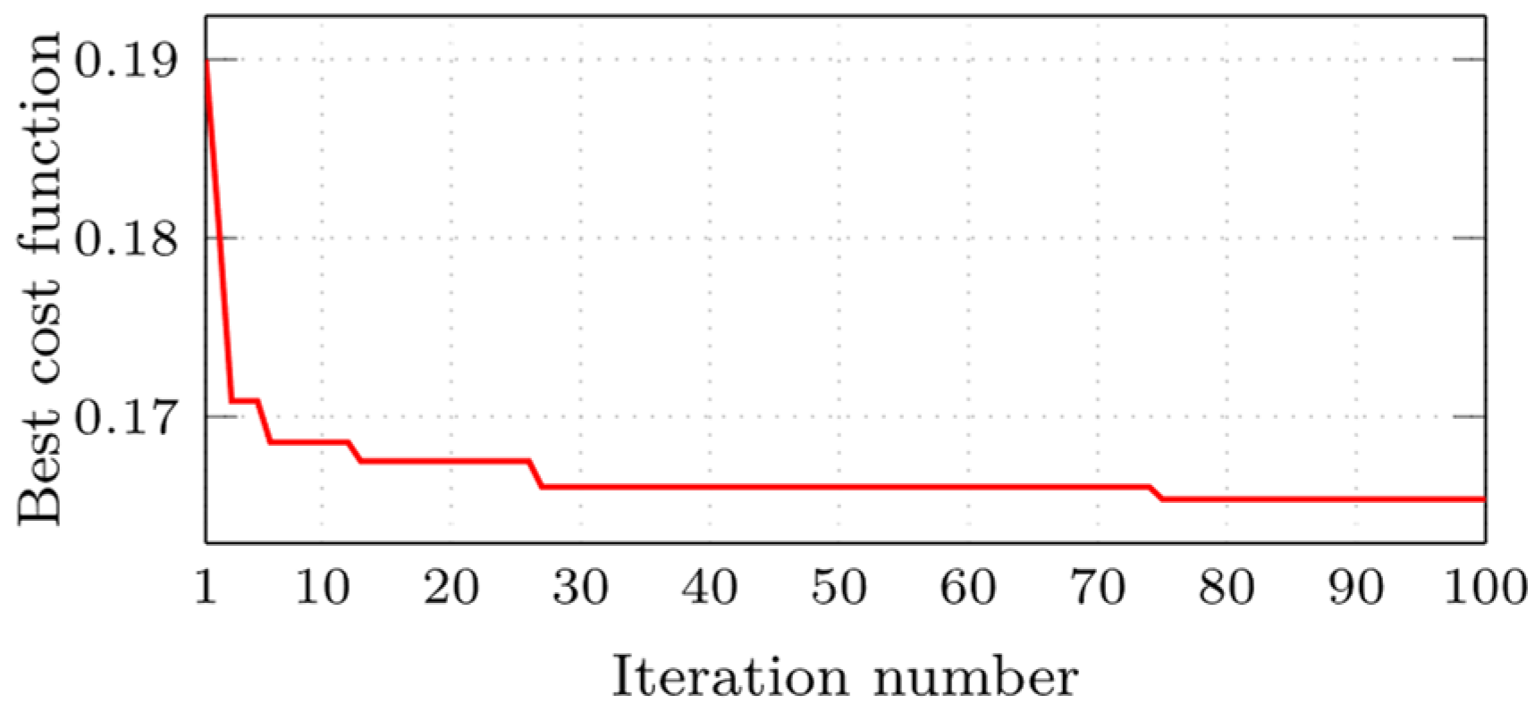
  • The metaheuristic optimization approach (GWO) has been implemented to find the optimal gains of the proposed FO-MFPC controller.
  • The performance of the proposed system utilizing the FO-MFPC controller and the conventional MFPC has been compared. The controller’s performance has been tested under linear and nonlinear load disturbances.
  • The robustness of the proposed control system under parameter uncertainty has been discussed.
  • The effect of changing the sampling period on the system performance has been studied and compared for the proposed FO-MFPC controller and the conventional MFPC.
The manuscript is arranged as follows. First, the conventional model-free predictive control based on the ultra-local model is explained in Section 2. Then, in Section 3, the proposed fractional-order model-free predictive control is described. Next, Section 4 discusses the simulation results. Finally, Section 5 presents the research conclusions.

2. Conventional Model-Free Predictive Control of UPS Based on an Ultra-Local Model

Figure 1 shows a 3-Φ VSI power circuit with the conventional MFPC controller. The converter is connected to a load via an LC filter to eliminate the current’s low-order harmonics and provide a sinusoidal 3-Φ voltage at the load terminals. All of the circuit 3-Φ variables, such as (va, vb, and vc), are represented by the space vector (Vx,αβ) notation:
V x , α β = 2 / 3 ( v a + e j ( 2 π / 3 ) v b + e j ( 4 π / 3 ) v c )
The three-phase 2L-VSI has six switched devices ( S 1 :   S 6 ) with eight possible switching states (i.e., 2^3), as listed in Table 1, in which Vdc is the value of the input dc source. The space vectors of the inverter output voltage (Vx,αβ) during the eight switching states (x ∈ [0, 7]) are shown in Figure 2. The space vector diagram is evidently comprised of six distinct sectors. In this space vector modeling, there are a total of eight vectors, out of which two are zero vectors, and the remaining six are referred to as active vectors. During the active vectors, the DC source and load are exclusively connected through a direct path. More details about the conventional MPC for the three-phase 2L-VSI in UPS applications can be found in [32].
Figure 3 depicts the fundamental building blocks of the ULM. The symbol F is the unknown function or variable in the ULM that includes the system’s overall uncertainty and disruption [33]. The system output and preceding control input are measured in order to define this unknown function F. In addition, the ULM principle can be expressed as follows:
y ( n ) = F + α u
where y ( n ) denotes the nth derivative of y (i.e., in most cases, the practitioner chooses either 1 or 2, with 1 being the most frequently chosen option in all actual circumstances) [20], u indicates the input of the controlled plant, y denotes the plant output, and α ∈ R stands for a non-physical parameter.
When using algebraic identification approaches, the value of F can be substituted with a more exact number in place of the estimate by using the letter F ^ . Finally, the value of F ^ may be determined using the Heun technique as follows [34]:
F ^ = 3 N f 3 T s i = 1 N f ( F 1 + F 2 )
where
F 1 = ( N f 2 ( i 1 ) ) y ( k 1 ) + ( N f 2 i ) y ( k )
F 2 = ( α ( i 1 ) T s ( N f ( i 1 ) ) ) u ( k 1 ) + α i T s ( N f i ) u ( k )
where Nf is the length of the window and k is the current instant of the variable.
More specifically, in the case of the UPS, the control target is the output voltage, so the ULM for the VSI with the UPS is given by:
d V o , α β ( k ) d t = F ^ α β + α u α β
where V o , α β ( k ) is the output voltage in the (αβ) coordination frame at kth instant; u α β is the optimal voltage vector from Table 1, which is applied at the instant k in the (αβ) coordination frame; and F ^ α β is the (αβ) component of the approximated unknown function F ^ .
The MFPC model can predict the output voltage at different voltage vectors Vx when applied in the next sampling interval. Euler theory can be used to solve the differential term in Equation (4) and obtain the discrete equation that can be used to predict the output voltage at any given voltage vector as below:
V o , α β ( k + 1 ) = V o , α β ( k ) + T s ( F ^ α β + α V x , α β ( k + 1 ) )
where V o , α β ( k + 1 ) is the predicted voltage across the capacitor Cf in the (αβ) coordination frame, V o , α β ( k ) is the measured output voltage, V x , α β ( k + 1 ) is the voltage vector from Table 1 and Equation (1), and Ts is the sampling period.
The multi-objective optimization of the MFPC aims to minimize the total cost functional at any voltage vector x from Table 1, which includes two terms with equal priority as in Equation (6). Consequently, the employed cost function does not need to use weighting factors as we only have one objective: the inverter output voltage. This introduces a flexible algorithm with enhanced power quality.
g ( x ) = ( V r e f , α ( k + 1 ) V o , α ( k + 1 ) ) 2 + ( V r e f , β ( k + 1 ) V o , β ( k + 1 ) ) 2
where Vref,α (k + 1) and Vref,β(k + 1) are the reference voltages in the (αβ) coordination frame and Vo,α (k + 1) and Vo,β (k + 1) are the predicted output voltages in the (αβ) coordination frame.

3. Proposed Fractional-Order Model-Free Predictive Control

3.1. Fractional-Order Calculus

When using fractional operators in the controller, every real number may be represented as a generic differential or integral notation [34]. The fundamental mathematical relationship of the FO differential or integral operators can be written as follows:
D l b , u b q f ( t ) = { d q d t q   f ( t ) q > 0 f ( t ) q = 0 l b u b f ( t ) d τ q q < 0
where q is the order of the FO calculus, lb and ub denote the lower and upper bands, respectively. It is clear that when the order is positive (i.e., q > 0), it is considered FO differential. On the other hand, when the order is negative (i.e., q < 0), it is considered FO integral. There are two different ways to figure out the principle of the FO. One is to use the Riemann–Liouville (R-L), which helps to derive the order derivative of a function f(t) [35]:
D l b , u b q f ( t ) = 1 Γ ( n q ) ( d d t ) n l b u b f ( τ ) ( t τ ) q n + 1 d τ
where Γ ( w ) = 0 t w 1 e t d t is the Gamma function, n ∈ N, and n − 1 < q < n.
The Laplace technique may be used to translate the fractional derivative of R-L found in Equation (8) to obtain the solution in Equation (9) [34]. We may also express the time domain representation of the q order of the function f(t) by using the definition of Caputo, which is a second definition connected to the idea of FO, as indicated in Equation (10).
{ D 0 q f ( t ) } = s q F ( s ) z = 0 n 1 s z ( D 0 q z 1 f ( t ) ) | t = 0
D l b , u b q f ( t ) = { 1 Γ ( n q ) ( l b u b f n ( τ ) ( t τ ) 1 n + q d τ ) n 1 < q < n ( d d t ) n f ( t ) q = n
Applying the Laplace transformation to Equation (10), the integral order has an initial condition, which indicates its physical meaning, as described in Equation (11):
{ D 0 q f ( t ) } = s q F ( s ) z = 0 n 1 s q z 1 f ( z ) ( 0 )
where s is the Laplace operator.
A FOPI controller has three parameters: the proportional gain Kp, integral gain Ki, and integral fractional order λ, as presented in Figure 4. In addition, the complete transfer function of the FOPI in Laplace form, Gc(s), is given in Equation (12). It has been found that controllers built using these specific parameters can have improved transient time, stability, and overall accuracy compared to traditional PI controllers. Additionally, the controller provides more flexibility and resilience when dealing with system disturbances. This allows it to handle a wide range of disturbances.
G c ( s ) = K p + K i ( 1 s ) λ
where λ is frequently in the range of [0, 1].

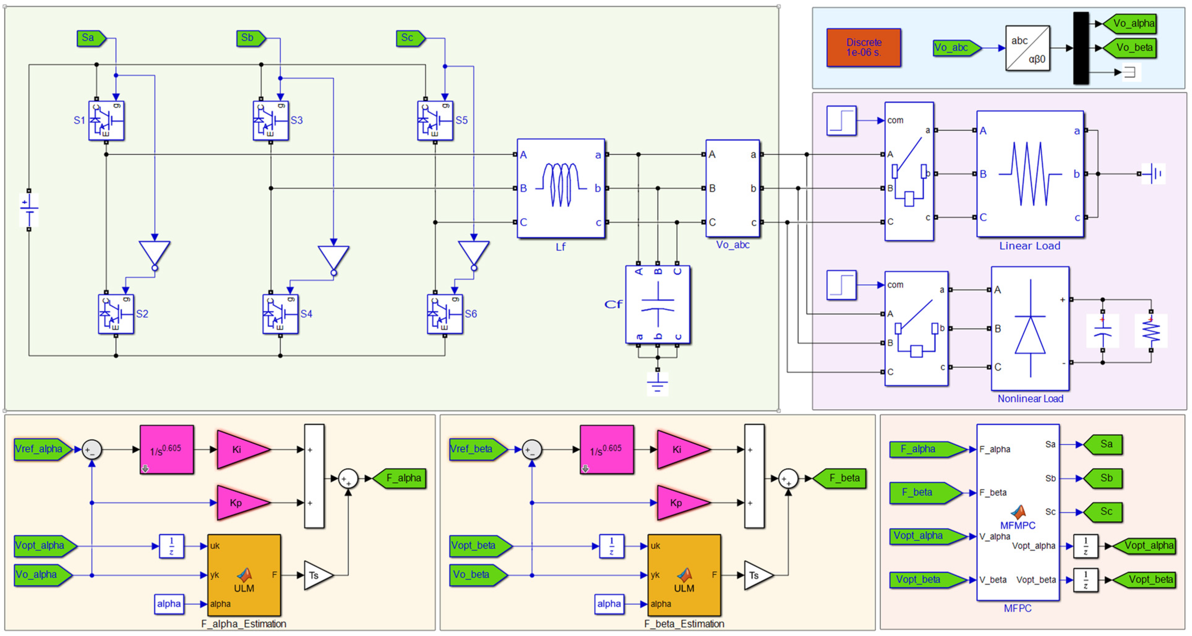
3.2. Proposed FO-MFPC for 2L-VSI in UPS Applications

The main idea behind the proposed FO-MFPC is to enhance the calculations of the unknown function F ^ compared to the algebraic identification with the conventional MFPC. The algebraic estimation for the function F ^ in the conventional MFPC will be added to the output of the FOPI controller, resulting in a modified F ^ (i.e., F ^ m,αβ) as in Equation (13). This could help improve the rejection of disturbances caused by load changes and parameter mismatches.
F ^ m , α β = T s F ^ α β + ( V r e f , α β ( k ) V o , α β ( k ) ) × ( K p + K i ( 1 s ) λ )
Then, the value of future output voltage across the capacitor of the filter by which the trajectory of the load voltage could be predicted is given as:
V o , α β ( k + 1 ) = V o , α β ( k ) + T s ( F ^ m , α β + α V x , α β ( k + 1 ) )
The complete structure of the proposed FO-MFPC is shown in Figure 5. First, the algebraic estimation of F is obtained using Equation (3) and updated every sampling interval Ts. Using this value, the predicted value of 2L-VSI at different possible voltage vectors can be calculated with Equation (5). Then, the cost function is evaluated to select the switching vector that provides the minimum value. Implementing the proposed FO-MFPC can be time-consuming, but more feasible as digital signal processors (DSPs) become more powerful. Additionally, a multiple-step prediction can decrease the influence of computational delay on control performance [36].
The complete flowchart of the proposed FO-MFPC for 2L-VSI is depicted in Figure 6. The entire procedure of the proposed FO-MFPC for 2L-VSI can be described step-by-step as follows:
(1)
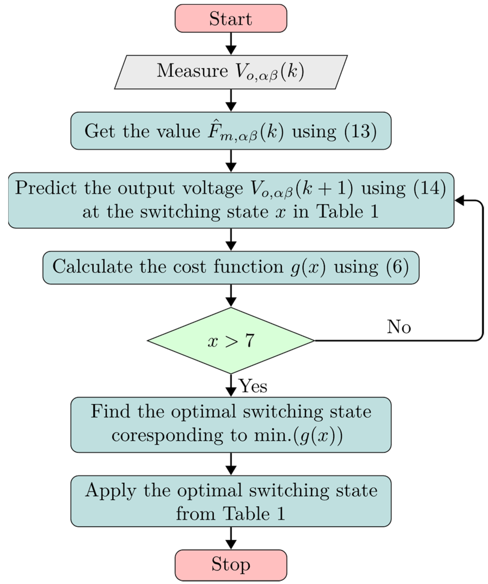
At sampling instant k, the controlled variables (Vo,αβ(k)) should be measured.
(2)
Those controlled variables are then predicted at instant k + 1 based on the discrete model of the converter given in Equation (14).
(3)
After defining a proper cost function g(x), as in Equation (6), it should be calculated for the current switching states (x) based on the desired value of the controlled variable.
(4)
As the main objective of the optimization problem is to find the optimum switching state that minimizes the cost function, the cost function of the current switching state g(x) is compared with the smallest previous value.
(5)
Steps (2) to (4) are repeated for all possible switching states given in Table 1.
(6)
Finally, the optimum switching state is applied at the next sampling instant.
The FOPI parameters can be established by trial and error, which can be challenging and dependent on the practitioner’s experience. Finding the right values for the proposed FO-MFPC parameters can be challenging. Still, it is crucial to carry it out in a manner that improves system performance and guarantees system stability against interruptions. A metaheuristic optimization technique based on GWO is utilized to determine the optimal value for the parameters of the FOPI controller.
Figure 7 depicts the FOPI parameters’ tuning procedure. The GWO algorithm runs on a personal computer employing an Intel© Core™ i5-8265U processor operating at 1.60 GHz and 16 GB of RAM. The GWO will keep going around 100 times, and the grey wolf’s number will be 20. The minimum range of the parameters is [−1,−1,0.1], while the maximum range is [1,1,1]. The employed fitness function for the GWO is the integral square error (ISE) as in Equation (15). The convergence curve of the employed GWO is shown in Figure 8, and the optimal parameters of the FOPI are summarized in Table 2. The proposed GWO algorithm achieves a small fitness function value of approximately 0.156. In addition, the GWO algorithm nearly finds the optimal parameters after 80 iterations for the ISE objective function. The parameter α is selected before running the GWO algorithm in order to ensure optimal FOPI gains at the current system parameter setting of the ULM.
I S E = 0 t s i m ( ( V r e f , α ( k ) V o , α ( k ) ) 2 + ( V r e f , β ( k ) V o , β ( k ) ) 2 )   d t
where t s i m is the simulation time.

4. Simulation Results

The proposed VSI with the investigated FO-MFPC controller, as shown in Figure 5, is simulated using MATLAB. The proposed system’s technical parameters are presented in Table 3, while Figure 9 shows the Simulink modeling for the simulation results. The proposed system has been tested under three circumstances to investigate the benefits of the control system. The first case tests the steady-state response of the proposed system under a linear resistive load. The system’s transient response under a step resistive load change is verified in the second case. In the third case, the steady-state response of the proposed system under nonlinear load has been tested. The performance of the proposed FO-MFPC controller is compared to that of the conventional MFPC for the three loading cases. Discussions and comparisons of the results are presented in the following paragraphs.

4.1. Case 1: Steady-State Response @ Linear Resistive Load

In this case, the system’s steady-state performance is demonstrated by the inverter load, which is a linear resistive load. Figure 10 displays the system’s steady-state performance utilizing the proposed FO-MFPC controller and a traditional MFPC controller. For both controllers, the 3-Φ load currents are shown in Figure 10a,b. It is seen that the currents for the two controllers are sinusoidal and balanced. Additionally, as illustrated in Figure 10c,d, the output 3-Φ voltage for both controllers is sinusoidal and balanced. However, the typical MFPC controller’s output voltage has a little bit more ripple. The αβ components of the output voltage compared to their reference values are presented in Figure 10e,f. Additionally, the performance of the proposed FO-MFPC controller is better than that of the conventional one in tracking the reference signals. The controller’s measured unknown function, which contains all the system disturbances [37,38], is presented in Figure 10g,h. It is noted that the function has serious disturbances and noise in the case of the conventional MFPC controller. Figure 10i,j present the voltage harmonic spectrum for the two controllers. The harmonic spectrum and the THD of the proposed controller are the best. Therefore, the overall response of the VSI with the proposed FO-MFPC controller is better than that with the conventional MFPC controller.

4.2. Case 2: Transient Response @ Step Resistive Load Change

In this case, the inverter load is a linear resistive load with a step change to present the transient state performance of the system. The transient performance of the system using the proposed FO-MFPC controller and the conventional MFPC controller is shown in Figure 11. The load step is applied at 0.07 s. Figure 11a,b show the 3-Φ load currents for both controllers. It is noticed that the currents are sinusoidal and balanced for the two controllers. The currents encounter some transients with each controller. However, the transients have a lower amplitude, ~50%, and shorter time, ~30%, in the case of the proposed controller. Additionally, the output 3-Φ voltages for both controllers have a sinusoidal and balanced nature, as shown in Figure 11c,d. As a result of the presence of the filter inductance, the current transients produce a transient distortion in the output voltage waves. Nevertheless, the output voltage in the case of the conventional MFPC controller has slightly higher transient distortions. The transient responses of the αβ components of the output voltage compared to their reference values are presented in Figure 11e,f. Additionally, the performance of the proposed FO-MFPC controller is better than that of the conventional one in tracking the reference signals and the transient response. The error between the output voltage and its reference value in the αβ frame is shown in Figure 11g,h. It is clear that the proposed FO-MFPC achieves the minimum error compared to the conventional MFPC. The controller’s unknown functions are presented in Figure 11i,j. It is noted that the function has high noise and spikes in the case of the conventional MFPC controller. The overall transient response of the VSI with the proposed FO-MFPC controller is better than that with the conventional MFPC controller.

4.3. Case 3: Steady-State Response @ Nonlinear Load

In this case, the inverter load is nonlinear and consists of a three-phase rectifier and a filtered capacitor at the output terminal with a 200 µF capacitance. The load resistance, in this case, is 100 Ω. The system steady state performance using the proposed FO-MFPC controller and conventional MFPC controller is shown in Figure 12. Figure 12a,b show the 3-Φ load currents for both controllers. It is noticed that the currents are highly distorted, far from sinusoidal waves, and unbalanced for the two controllers. However, the output 3-Φ voltages for both controllers have a sinusoidal and balanced nature, as shown in Figure 12c,d. Nevertheless, the output voltage in the case of the conventional MFPC controller has slightly higher ripples. The unknown function in the controller that contains all the disturbances in the system is presented in Figure 12e,f. It is noted that the function has higher noise in the case of the conventional MFPC controller. Therefore, the overall response of the VSI, which supplies the nonlinear load, with the proposed FO-MFPC controller is better than that with the conventional MFPC controller.

4.4. Case 4: Parameter Mismatch

To check the robustness of the control system under parameter uncertainty, the effect of a 50% change in the filter capacitor value (Cf) on VSI performance with the two controllers is presented in Figure 13. It is noted that the two controllers track the reference signals well. This shows the robustness of the two control systems against parameter mismatches. On the other hand, the THD of the output voltage shows a small relative increase between the two controllers.

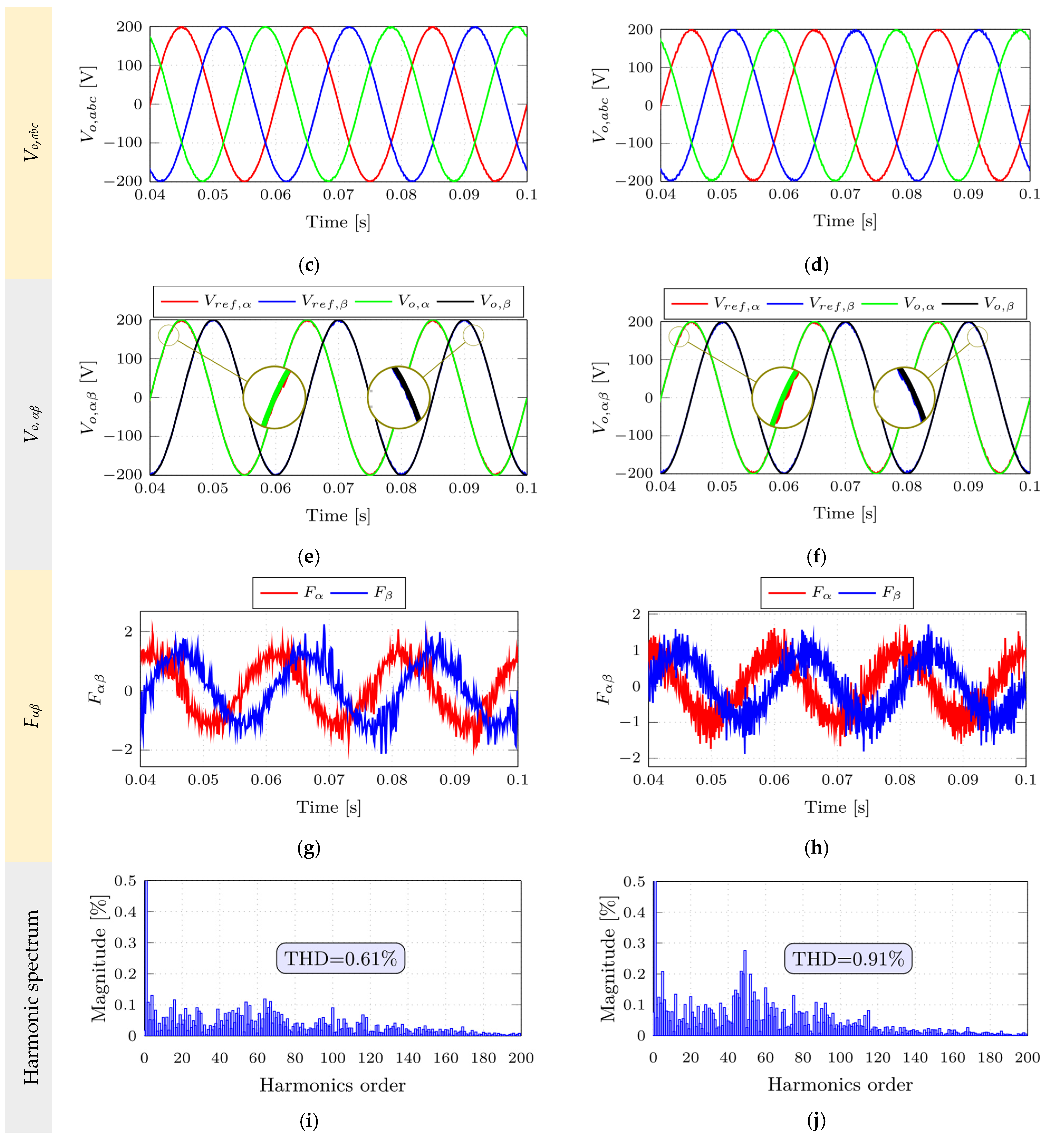
4.5. THD Evaluation at Different Sampling Intervals

The effect of varying the sampling period on the performance of the VSI controlled using the proposed FO-MFPC and the conventional MFPC has been studied. Figure 14 compares the output voltage THD for the two controllers at different sampling periods. The THDs using the two controllers are lower than the standard recommended values [39]. As expected, the THD using the two controllers increased with the sampling period. However, it is clear that the proposed FO-MFPC controller usually has the lowest THD for any sampling time. The minimum decrease in the THD when using the proposed controller is 10% and the maximum is 48%.

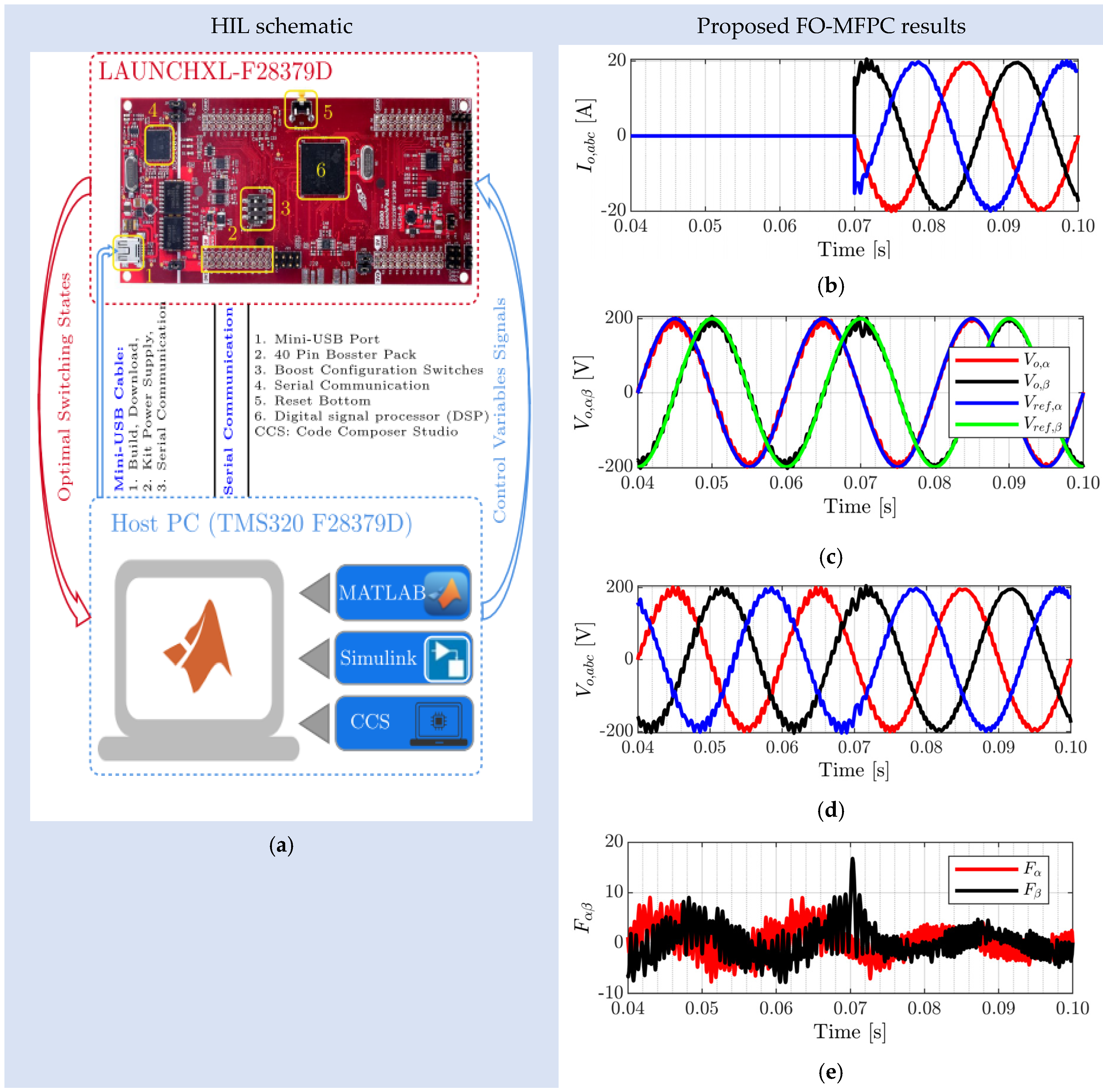
4.6. HIL Validation Results

The C2000TM-microcontroller-LaunchPadXL TMS320F28379D kit has been constructed as a Hardware-in-the-Loop (HIL) emulator to test the proposed system and confirm the researched simulation findings. The HIL emulator works by hosting a particular system component—typically the power component—in the computer as a MATLAB model. The MATLAB application simulates and hosts the planned system power units, such as the power converters and filters. On the other side, the micro-controller kit implements the control algorithms, namely, the proposed FO-MFPC. The virtual serial COM ports [6] facilitate the communication between the PC and the kit. It enables MATLAB to provide measured signals from the power circuit to the kit, including the DC bus voltage, load voltages, and load currents. To produce the 2L-VSI switching signals, the kit performs the control algorithms. Figure 15a shows a schematic diagram of the HIL implementation of the proposed 2L-VSI.
Figure 15b–e presents the results of the HIL validation of the proposed 2L-VSI with FO-MFPC for case (2): the inverter load is a linear resistive load with a step change to present the transient state performance of the system. The load currents and voltages are very close to the simulations results except for some contaminated noise on the waveforms. It is noted that the signals have higher noise and spikes in the case of the HIL implementation than the simulation results of Figure 11.

5. Conclusions

This paper proposes employing the fractional-order controller to improve the performance of the MFPC of the 2L-VSI voltage control in UPS applications. The proposed FO-MFPC uses fractional-order proportional-integral control (FOPI) to estimate the unknown function associated with the MFPC. To get the best performance from FOPI, its parameters are optimally designed using the GWO approach. For three loading cases and conditions, the performance of the proposed FO-MFPC controller is compared to that of the conventional MFPC. Using MATLAB simulations, the simulation results indicated the superiority of the proposed FO-MFPC controller over the conventional MFPC in steady state and transient responses. The results indicated that the THD of the output voltage for the two controllers is much lower than the recommended standard. However, the THD with the proposed FO-MFPC controller is lower than that with the conventional MFPC controller. Additionally, it has been noticed that the proposed FO-MFPC controller usually has the lowest THD. The suggested controller can reduce the THD by as little as 10% and as much as 48%. To check the robustness of the control system under parameter uncertainty, the effect of a 50% change in the filter capacitor value on the performance of the VSI has been determined. The results prove the robustness of the two control systems against parameter mismatches. Moreover, the effect of varying the sampling period on the performance of the VSI controlled using the proposed FO-MFPC and the conventional MFPC has been studied. As expected, the THD using the two controllers increased with the sampling period increase and the proposed FO-MFPC controller has the lowest THD for any sampling time. The future work of the paper could focus on employing the fuzzy logic controller to enhance the calculations of the disturbance function associated with the ULM. Additionally, using the TMS320F28379D kit, the experimental verification of the proposed FO-MFPC control strategy is implemented for 2L-VSI on the basis of the HIL simulator, demonstrating the applicability and effective performance of our proposed control strategy under realistic circumstances.

Author Contributions

A.B. (Abualkasim Bakeer) designed the system, and S.A.Z. derived the model and analyzed the results. H.A. helped in writing the paper. E.-H.A., A.E., A.B. (Ahmed Bensenouci), and M.A. supported the funding process. All authors have read and agreed to the published version of the manuscript.

Funding

This research was funded by Deputyship for Research and Innovation, Ministry of Education in Saudi Arabia, Grant Number 0029-1442-S.

Data Availability Statement

Data are available from the authors upon reasonable request.

Acknowledgments

The authors extend their appreciation to the Deputyship for Research and Innovation, Ministry of Education in Saudi Arabia for funding this research work through the project number (0029-1442-S). The authors also acknowledge the support of the Deanship of Scientific Research at the University of Tabuk.

Conflicts of Interest

The authors declare no conflict of interest.

Nomenclature

2L-VSITwo-level voltage source inverter
FOCFractional-order controller
MFPCModel-free predictive control
UPSUninterruptable power supply
ULMUltra-local model
FOPIFractional-order proportional-integral
GWOGrey wolf optimization
THDTotal harmonics distortion
FCS-MPCFinite control set-model predictive control
PWMPulse width modulation
LCInductor-capacitor
V x 
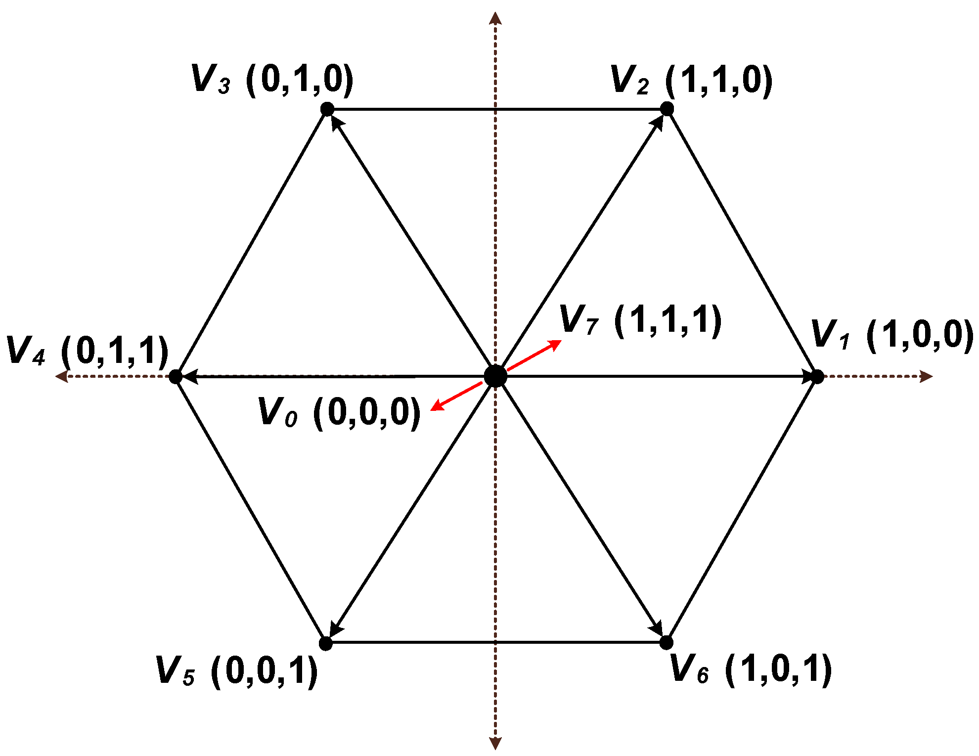
Space voltage vector
FUnknown function associated with MFPC
uPlant input
yPlant output
αNon-physical parameter
TsSampling time
NfLength of the window
F ^ Approximated value of the unknown function F
CfFilter capacitor
xVoltage vector number in Table 1
FOFractional-order
qOrder of the FO calculus
lbLower band of the FO integrator
ubUpper band of the FO integrator
R-LRiemann–Liouville
KpProportional gain of the FOPI
KiIntegral gain of the FOPI
λIntegral fractional order
PIProportional integral
Gc(s)FOPI transfer function
sLaplace operator
F ^ m,αβModified value of the unknown function F ^ αβ
ISEIntegral square error

References

  1. Yan, S.; Yang, Y.; Hui, S.Y.; Blaabjerg, F. A Review on Direct Power Control of Pulsewidth Modulation Converters. IEEE Trans. Power Electron. 2021, 36, 11984–12007. [Google Scholar] [CrossRef]
  2. Padmanaban, S.; Samavat, T.; Nasab, M.A.; Nasab, M.A.; Zand, M.; Nikokar, F. Electric Vehicles and IoT in Smart Cities. Artif. Intell.-Based Smart Power Syst. 2023, 273–290. [Google Scholar]
  3. Khalili, M.; Dashtaki, M.A.; Nasab, M.A.; Hanif, H.R.; Padmanaban, S.; Khan, B. Optimal instantaneous prediction of voltage instability due to transient faults in power networks taking into account the dynamic effect of generators. Cogent. Eng. 2022, 9, 2072568. [Google Scholar] [CrossRef]
  4. Zaid, S.A.; Albalawi, H.; AbdelMeguid, H.; Alhmiedat, T.A.; Bakeer, A. Performance Improvement of H8 Transformerless Grid-Tied Inverter Using Model Predictive Control Considering a Weak Grid. Processes 2022, 10, 1243. [Google Scholar] [CrossRef]
  5. Ahmed, A.; Biswas, S.P.; Anower, S.; Islam, R.; Mondal, S.; Muyeen, S.M. A Hybrid PWM Technique to Improve the Performance of Voltage Source Inverters. IEEE Access 2023, 11, 4717–4729. [Google Scholar] [CrossRef]
  6. Zaid, S.A.; Mohamed, I.S.; Bakeer, A.; Liu, L.; Albalawi, H.; Tawfiq, M.E.; Kassem, A.M. From MPC-Based to End-to-End (E2E) Learning-Based Control Policy for Grid-Tied 3L-NPC Transformerless Inverter. IEEE Access 2022, 10, 57309–57326. [Google Scholar] [CrossRef]
  7. Albalawi, H.; Zaid, S.A. Performance Improvement of a Grid-Tied Neutral-Point-Clamped 3-φ Transformerless Inverter Using Model Predictive Control. Processes 2019, 7, 856. [Google Scholar] [CrossRef]
  8. De Bén, A.A.E.; Alvarez-Diazcomas, A.; Rodriguez-Resendiz, J. Transformerless Multilevel Voltage-Source Inverter Topology Comparative Study for PV Systems. Energies 2020, 13, 3261. [Google Scholar] [CrossRef]
  9. Yuan, W.; Wang, T.; Diallo, D.; Delpha, C. A Fault Diagnosis Strategy Based on Multilevel Classification for a Cascaded Photovoltaic Grid-Connected Inverter. Electronics 2020, 9, 429. [Google Scholar] [CrossRef]
  10. Rana, R.A.; Patel, S.A.; Muthusamy, A.; Lee, C.W.; Kim, H.-J. Review of Multilevel Voltage Source Inverter Topologies and Analysis of Harmonics Distortions in FC-MLI. Electronics 2019, 8, 1329. [Google Scholar] [CrossRef]
  11. Anwar, M.A.; Abbas, G.; Khan, I.; Awan, A.B.; Farooq, U.; Khan, S.S. An Impedance Network-Based Three Level Quasi Neutral Point Clamped Inverter with High Voltage Gain. Energies 2020, 13, 1261. [Google Scholar] [CrossRef]
  12. Heredero-Peris, D.; Chillón-Antón, C.; Sánchez-Sánchez, E.; Montesinos-Miracle, D. Fractional proportional-resonant current controllers for voltage source converters. Electr. Power Syst. Res. 2018, 168, 20–45. [Google Scholar] [CrossRef]
  13. Carlet, P.G.; Tinazzi, F.; Bolognani, S.; Zigliotto, M. An Effective Model-Free Predictive Current Control for Synchronous Reluctance Motor Drives. IEEE Trans. Ind. Appl. 2019, 55, 3781–3790. [Google Scholar] [CrossRef]
  14. Mohamed, I.S.; Rovetta, S.; Do, T.D.; Dragicevi´c, T.; Diab, A.A.Z. A neural-network-based model predictive control of three-phase inverter with an output LC filter. IEEE Access 2019, 7, 124737–124749. [Google Scholar] [CrossRef]
  15. Mohamed-Seghir, M.; Krama, A.; Refaat, S.S.; Trabelsi, M.; Abu-Rub, H. Artificial Intelligence-BasedWeighting Factor Autotuning for Model Predictive Control of Grid-Tied Packed U-Cell Inverter. Energies 2020, 13, 3107. [Google Scholar] [CrossRef]
  16. Lucia, S.; Navarro, D.; Karg, B.; Sarnago, H.; Lucia, O. Deep Learning-Based Model Predictive Control for Resonant Power Converters. IEEE Trans. Ind. Inform. 2020, 17, 409–420. [Google Scholar] [CrossRef]
  17. Fliess, M.; Join, C. Model-free control. Int. J. Control 2013, 86, 2228–2252. [Google Scholar] [CrossRef]
  18. Stenman, A. Model-free predictive control. Proc. 38th IEEE Conf. Decis. Control. 1999, 4, 3712–3717. [Google Scholar]
  19. Rodriguez, J.; Heydari, R.; Rafiee, Z.; Young, H.A.; Flores-Bahamonde, F.; Shahparasti, M. Model-Free Predictive Current Control of a Voltage Source Inverter. IEEE Access 2020, 8, 211104–211114. [Google Scholar] [CrossRef]
  20. Zhang, Y.; Liu, X.; Liu, J.; Rodriguez, J.; Garcia, C. Model-Free Predictive Current Control of Power Converters Based on Ultra-Local Model. IEEE Int. Conf. Industrial Technol. (ICIT) 2020, 1089–1093. [Google Scholar] [CrossRef]
  21. Khalilzadeh, M.; Vaez-Zadeh, S.; Rodriguez, J.; Heydari, R. Model-Free Predictive Control of Motor Drives and Power Converters: A Review. IEEE Access 2021, 9, 105733–105747. [Google Scholar] [CrossRef]
  22. Wang, S.; Li, J.; Hou, Z.; Meng, Q.; Li, M. Composite Model-free Adaptive Predictive Control for Wind Power Generation Based on Full Wind Speed. CSEE J. Power Energy Syst. 2022, 8, 1659–1669. [Google Scholar] [CrossRef]
  23. Sabzevari, S.; Heydari, R.; Mohiti, M.; Savaghebi, M.; Rodriguez, J. Model-Free Neural Network-Based Predictive Control for Robust Operation of Power Converters. Energies 2021, 14, 2325. [Google Scholar] [CrossRef]
  24. Yin, Z.; Hu, C.; Luo, K.; Rui, T.; Feng, Z.; Lu, G.; Zhang, P. A Novel Model-Free Predictive Control for T-Type Three-Level Grid-Tied Inverters. Energies 2022, 15, 6557. [Google Scholar] [CrossRef]
  25. Zhang, Y.; Liu, J. An improved model-free predictive current control of pwm rectifiers. In Proceedings of the 20th International Conference on Electrical Machines and Systems (ICEMS), Sydney, Australia, 11–14 August 2017; pp. 1–5. [Google Scholar]
  26. Fliess, M.; Join, C. Model-free control and intelligent pid controllers: Towards a possible trivialization of nonlinear control? IFAC Proc. Vol. 2009, 42, 1531–1550. [Google Scholar] [CrossRef]
  27. Birs, I.; Muresan, C.; Nascu, I.; Ionescu, C. A Survey of Recent Advances in Fractional Order Control for Time Delay Systems. IEEE Access 2019, 7, 30951–30965. [Google Scholar] [CrossRef]
  28. Traver, J.E.; Nuevo-Gallardo, C.; Tejado, I.; Fernández-Portales, J.; Ortega-Morán, J.F.; Pagador, J.B.; Vinagre, B.M. Cardiovascular Circulatory System and Left Carotid Model: A Fractional Approach to Disease Modeling. Fractal Fract. 2022, 6, 64. [Google Scholar] [CrossRef]
  29. Shah, P.; Agashe, S. Review of fractional PID controller. Mechatronics 2016, 38, 29–41. [Google Scholar] [CrossRef]
  30. Nazir, R. Taylor series expansion based repetitive controllers for power converters, subject to fractional delays. Control Eng. Pract. 2017, 64, 140–147. [Google Scholar] [CrossRef]
  31. Pullaguram, D.; Mishra, S.; Senroy, N.; Mukherjee, M. Design and Tuning of Robust Fractional Order Controller for Autonomous Microgrid VSC System. IEEE Trans. Ind. Appl. 2017, 54, 91–101. [Google Scholar] [CrossRef]
  32. Bakeer, A.; Alhasheem, M.; Peyghami, S. Efficient Fixed-Switching Modulated Finite Control Set-Model Predictive Control Based on Artificial Neural Networks. Appl. Sci. 2022, 12, 3134. [Google Scholar] [CrossRef]
  33. Bakeer, A.; Magdy, G.; Chub, A.; Jurado, F.; Rihan, M. Optimal Ultra-Local Model Control Integrated with Load Frequency Control of Renewable Energy Sources Based Microgrids. Energies 2022, 15, 9177. [Google Scholar] [CrossRef]
  34. Zaid, S.A.; Bakeer, A.; Magdy, G.; Albalawi, H.; Kassem, A.M.; El-Shimy, M.E.; AbdelMeguid, H.; Manqarah, B. A New Intelligent Fractional-Order Load Frequency Control for Interconnected Modern Power Systems with Virtual Inertia Control. Fractal Fract. 2023, 7, 62. [Google Scholar] [CrossRef]
  35. Morsali, J.; Zare, K.; Hagh, M.T. Applying fractional order PID to design TCSC-based damping controller in coordination with automatic generation control of interconnected multi-source power system. Eng. Sci. Technol. Int. J. 2017, 20, 1–17. [Google Scholar] [CrossRef]
  36. Fawzy, A.; Bakeer, A.; Magdy, G.; Atawi, I.E.; Roshdy, M. Adaptive Virtual Inertia-Damping System Based on Model Predictive Control for Low-Inertia Microgrids. IEEE Access 2021, 9, 109718–109731. [Google Scholar] [CrossRef]
  37. Peng, Y.; Tang, S.; Huang, J.; Tang, C.; Wang, L.; Liu, Y. Fractal Analysis on Pore Structure and Modeling of Hydration of Magnesium Phosphate Cement Paste. Fractal Fract. 2022, 6, 337. [Google Scholar] [CrossRef]
  38. Tartaglione, V.; Farges, C.; Sabatier, J. Fractional Behaviours Modelling with Volterra Equations: Application to a Lithium-Ion Cell and Comparison with a Fractional Model. Fractal Fract. 2022, 6, 137. [Google Scholar] [CrossRef]
  39. ILangella, R.; Testa, A. AliiIEEE Recommended Practice and Requirements for Harmonic Control in Electric Power Systems; IEEE Std 519-2014 (Revision of IEEE Std 519-1992); IEEE: Piscataway, NJ, USA, 2014; pp. 1–29. [Google Scholar] [CrossRef]
Figure 1. The UPS-based 2L-VSI power circuit with the conventional MFPC controller.
Fractalfract 07 00433 g001
Figure 2. Space vectors of the output voltage at the 2L-VSI terminals.
Fractalfract 07 00433 g002
Figure 3. The basic implementation of the ULM.
Fractalfract 07 00433 g003
Figure 4. The FOPI controller’s fundamental structure.
Fractalfract 07 00433 g004
Figure 5. Structure of the proposed FO-MFPC of the 2L-VSI for UPS applications.
Fractalfract 07 00433 g005
Figure 6. Flowchart of the proposed FO-MFPC for one sampling interval.
Fractalfract 07 00433 g006
Figure 7. The tuning procedure of the proposed FO-MFPC for UPS.
Fractalfract 07 00433 g007
Figure 8. Convergence curve of the employed GWO to tune the FOPI gains of the proposed FO-MFPC.
Fractalfract 07 00433 g008
Figure 9. Simulink model of the proposed FO-MFPC for 2L-VSI.
Fractalfract 07 00433 g009
Figure 10. Steady-state response @ fixed resistive load for the UPS with the proposed FO-MFPC and conventional MFPC.
Fractalfract 07 00433 g010aFractalfract 07 00433 g010b
Figure 11. Transient response @ step changes from no-load to 20 A loading with the proposed FO-MFPC and conventional MFPC.
Fractalfract 07 00433 g011aFractalfract 07 00433 g011b
Figure 12. Steady-state response @ nonlinear load with the proposed FO-MFPC and conventional MFPC.
Fractalfract 07 00433 g012aFractalfract 07 00433 g012b
Figure 13. Mismatch of Cf with the proposed FO-MFPC and conventional MFPC.
Fractalfract 07 00433 g013
Figure 14. Comparisons of the THD at different sampling times of the proposed FO-MFPC and the conventional MFPC.
Fractalfract 07 00433 g014
Figure 15. The HIL validation of the proposed 2L-VSI: (a) the schematic diagram (be) the transient response @ step changes from no-load to 20 A loading using the proposed FO-MFPC.
Fractalfract 07 00433 g015
Table 1. Switching states of the 2L-VSI for UPS applications.
x V x Output Voltage Vx,αβ S 1 S 2 S 3 S 4 S 5 S 6
0V00000111
1V1 2 3 V d c 100011
2V2 1 3 V d c + j 3 3 V d c 110001
3V3 1 3 V d c + j 3 3 V d c 010101
4V4 2 3 V d c 011100
5V5 1 3 V d c j 3 3 V d c 001110
6V6 1 3 V d c j 3 3 V d c 101010
7V70111000
Table 2. The optimal parameters of the FO-MFPC using GWO.
ParameterValue
Kp0.360
Ki0.034
λ0.605
Table 3. Parameters of the studied 2L-VSI for UPS applications.
ParameterSymbolValue
Input voltageVdc500 V
Filter inductanceLf1.5 mH
Filter capacitanceCf150 µF
Nominal RMS output voltage (L-L)Vo,ref200 V
Sampling timeTs20 µs
Disclaimer/Publisher’s Note: The statements, opinions and data contained in all publications are solely those of the individual author(s) and contributor(s) and not of MDPI and/or the editor(s). MDPI and/or the editor(s) disclaim responsibility for any injury to people or property resulting from any ideas, methods, instructions or products referred to in the content.

