
New Versions of Midpoint Inequalities Based on Extended Riemann–Liouville Fractional Integrals


Abstract
:1. Introduction
2. Preliminaries
3. Main Outcomes
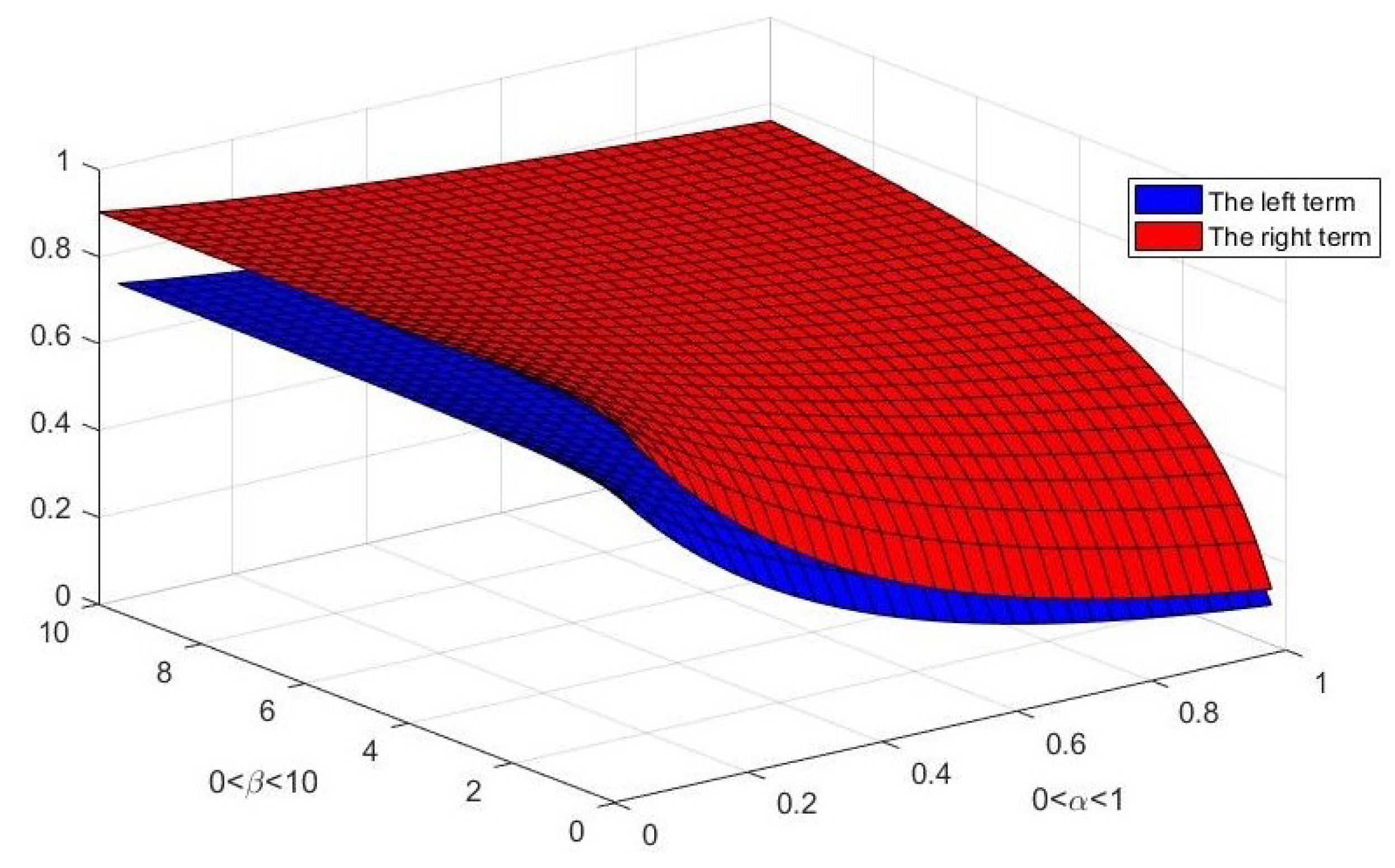
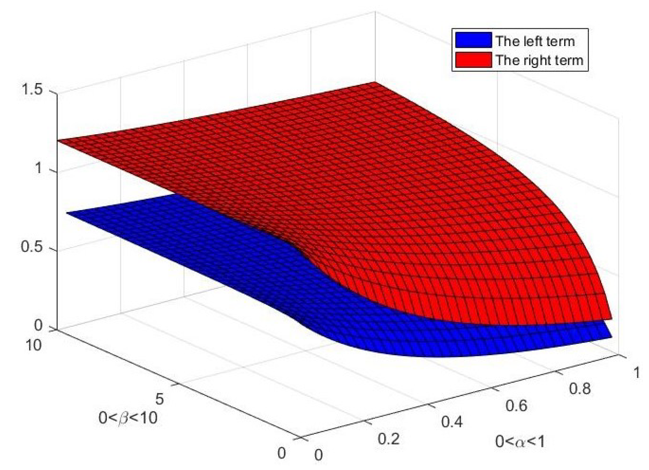
4. Examples
5. Conclusions
Author Contributions
Funding
Data Availability Statement
Acknowledgments
Conflicts of Interest
References
- Uchaikin, V.V. Fractional Derivatives for Physicists and Engineers; Springer: Berlin/Heidelberg, Germany, 2013. [Google Scholar]
- Baleanu, D.; Diethelm, K.; Scalas, E.; Trujillo, J.J. Fractional Calculus: Models and Numerical Methods; World Scientific: Singapore, 2016. [Google Scholar]
- Anastassiou, G.A. Generalized Fractional Calculus: New Advancements and Applications; Springer: Cham, Switzerland, 2021. [Google Scholar]
- Kilbas, A.A.; Srivastava, H.M.; Trujillo, J.J. Theory and Applications of Fractional Differential Equations, North-Holland Mathematics Studies; Elsevier Science B.V.: Amsterdam, The Netherlands, 2006; Volume 204. [Google Scholar]
- Magin, R.L. Fractional Calculus in Bioengineering; Begell House Publishers: Redding, CA, USA, 2006. [Google Scholar]
- Atangana, A.; Baleanu, D. New fractional derivative with non-local and non-singular kernel. Therm. Sci. 2016, 20, 757–763. [Google Scholar] [CrossRef]
- Sezer, S. The Hermite-Hadamard inequality for s-Convex functions in the third sense. AIMS Math. 2021, 6, 7719–7732. [Google Scholar] [CrossRef]
- Abdeljawad, T.; Baleanu, D. Integration by parts and its applications of a new nonlocal fractional derivative with Mittag-Leffler nonsingular kernel. J. Nonlinear Sci. Appl. 2017, 10, 1098–1107. [Google Scholar] [CrossRef]
- Krishna, V.; Maenner, E. Convex Potentials with an Application to Mechanism Design. Econometrica 2001, 69, 1113–1119. [Google Scholar] [CrossRef]
- Okubo, S.; Isihara, A. Inequality for convex functions in quantum-statistical mechanics. Physica 1972, 59, 228–240. [Google Scholar] [CrossRef]
- Peajcariaac, J.; Tong, Y. Convex Functions, Partial Orderings, and Statistical Applications; Academic Press: Cambridge, MA, USA, 1992. [Google Scholar]
- Murota, K.; Tamura, A. New characterizations of M-convex functions and their applications to economic equilibrium models with indivisibilities. Discret. Appl. Math. 2003, 131, 495–512. [Google Scholar] [CrossRef]
- Tariq, M.; Ahmad, H.; Sahoo, S.K.; Aljoufi, L.S.; Awan, S.K. A novel comprehensive analysis of the refinements of Hermite-Hadamard type integral inequalities involving special functions. J. Math. Comput. Sci. 2022, 26, 330–348. [Google Scholar] [CrossRef]
- Raees, M.; Anwar, M.; Farid, G. Error bounds associated with different versions of Hadamard inequalities of mid-point type. J. Math. Comput. Sci. 2021, 23, 213–229. [Google Scholar] [CrossRef]
- Hyder, A.; Barakat, M.A.; Fathallah, A.; Cesarano, C. Further Integral Inequalities through Some Generalized Fractional Integral Operators. Fractal Fract. 2021, 5, 282. [Google Scholar] [CrossRef]
- Sarikaya, M.Z.; Set, E.; Yaldiz, H.; Basak, N. Hermite—Hadamard’s inequalities for fractional integrals and related fractional inequalities. Math. Comput. Model. 2013, 57, 2403–2407. [Google Scholar] [CrossRef]
- Set, E. New inequalities of Ostrowski type for mappings whose derivatives are s-convex in the second sense via fractional integrals. Comput. Math. Appl. 2012, 63, 1147–1154. [Google Scholar] [CrossRef]
- Budak, H.; Hezenci, F.; Kara, H. On parameterized inequalities of Ostrowski and Simpson type for convex functions via generalized fractional integrals. Math. Methods Appl. Sci. 2021, 44, 12522–12536. [Google Scholar] [CrossRef]
- Hyder, A.; Budak, H.; Almoneef, A.A. Further midpoint inequalities via generalized fractional operators in Riemann-Liouville sense. Fractal Fract. 2022, 6, 496. [Google Scholar] [CrossRef]
- Hadamard, J. Etude sur les propriétés des fonctions entières et en particulier d’une fonction considérée par Riemann. J. Math. Pures Appl. 1893, 58, 171–215. [Google Scholar]
- Jarad, F.; Uğurlu, E.; Abdeljawad, T.; Baleanu, D. On a new class of fractional operators. Adv. Differ. Equ. 2017, 2017, 247. [Google Scholar] [CrossRef]
- Sarikaya, M.Z.; Yildirim, H. On Hermite-Hadamard type inequalities for Riemann-Liouville fractional integrals. Miskolc Math. Notes 2016, 7, 1049–1059. [Google Scholar] [CrossRef]
- Set, E.; Choi, J.; Gözpinar, A. Hermite–Hadamard Type Inequalities for New Conformable Fractional Integral Operator, Research- Gate Preprint. 2018. Available online: https://www.researchgate.net/publication/322936389 (accessed on 8 May 2012).
- Gözpınar, A. Some Hermite-Hadamard type inequalities for convex functions via new fractional conformable integrals and related inequalities. AIP Conf. Proc. 2018, 1991, 020006. [Google Scholar]
- Budak, H.; Kapucu, R. New generalization of midpoint type inequalities for fractional integral. An. Stiint¸. Univ. Al. I. Cuza Ia¸si. Mat. (N.S.) 2021. [Google Scholar] [CrossRef]
- Qaisar, S.; Hussain, S. On Hermite-Hadamard type inequalities for functions whose first derivative absolute values are convex and concave. Fasc. Math. 2017, 58, 155–166. [Google Scholar] [CrossRef]

Disclaimer/Publisher’s Note: The statements, opinions and data contained in all publications are solely those of the individual author(s) and contributor(s) and not of MDPI and/or the editor(s). MDPI and/or the editor(s) disclaim responsibility for any injury to people or property resulting from any ideas, methods, instructions or products referred to in the content. |
© 2023 by the authors. Licensee MDPI, Basel, Switzerland. This article is an open access article distributed under the terms and conditions of the Creative Commons Attribution (CC BY) license (https://creativecommons.org/licenses/by/4.0/).
Share and Cite
Hyder, A.-A.; Budak, H.; Barakat, M.A. New Versions of Midpoint Inequalities Based on Extended Riemann–Liouville Fractional Integrals. Fractal Fract. 2023, 7, 442. https://doi.org/10.3390/fractalfract7060442
Hyder A-A, Budak H, Barakat MA. New Versions of Midpoint Inequalities Based on Extended Riemann–Liouville Fractional Integrals. Fractal and Fractional. 2023; 7(6):442. https://doi.org/10.3390/fractalfract7060442
Chicago/Turabian StyleHyder, Abd-Allah, Hüseyin Budak, and Mohamed A. Barakat. 2023. "New Versions of Midpoint Inequalities Based on Extended Riemann–Liouville Fractional Integrals" Fractal and Fractional 7, no. 6: 442. https://doi.org/10.3390/fractalfract7060442