Dynamical Behaviour, Control, and Boundedness of a Fractional-Order Chaotic System

Abstract

In this paper, the fractional-order chaotic system form of a four-dimensional system with cross-product nonlinearities is introduced. The stability of the equilibrium points of the system and then the feedback control design to achieve this goal have been analyzed. Furthermore, further dynamical behaviors including, phase portraits, bifurcation diagrams, and the largest Lyapunov exponent are presented. Finally, the global Mittag–Leffler attractive sets (MLASs) and Mittag–Leffler positive invariant sets (MLPISs) of the considered fractional order system are presented. Numerical simulations are provided to show the effectiveness of the results.

1. Introduction

In recent years, fractional-order calculus has become a prominent part of applied research. Since applied sciences are naturally related to systems with memory, which dominates most physical and scientific systems, modeling with fractional order equations has been an undeniable necessity [1,2,3,4,5]. Fractional-order differential equations, which are actually generalizations of integer order calculus, deal with derivatives and integrals with non-integer orders. These equations have a unique feature which is the description of the memory effect [6,7,8]. Fractional derivative chaotic systems are now an important topic of study in nonlinear dynamics. The fractional-order chaotic system is considered a new alternative for which significant attention has been focused on developing techniques for modelling, synchronization, and control of the generalized dynamical systems [9,10,11,12,13]. Recently, fractional-order calculus has been applied to financial market changes. Investigations have indicated that economics and finance are extremely complex nonlinear systems involving many subjective factors, and there are many characteristics that cannot be modeled by integer-order calculus. Therefore, it is necessary to try to use the bifurcation and chaos of fractional nonlinear dynamics [14,15,16].

A chaotic system is a bounded nonlinear deterministic system with a long-term nature depending on the initial condition. The importance of the boundedness of a dynamical system can be found from the definition of chaos. Therefore, estimating the ultimate bound and positive invariant set of a chaotic system plays an important role in predicting its behavior, controlling chaos and preventing possible failures in physical and engineering systems. It can be clearly seen that the existence of the global attractor set for a system means the absence of hidden attractors outside this set [17,18,19,20].

By studying the ultimate bound of chaotic systems by Leonov [18], a new direction for research in this field was introduced. Many efforts have been made to develop methods for estimating the ultimate bound and the global attractive set of chaotic systems [21,22,23,24]. Despite many problems in determining the ultimate bound of some dynamical systems, various methods were presented that generally used optimization and the method of Lagrange coefficients [25,26,27]. Among the interesting studies that have been carried out so far, we can mention the calculation of the ultimate bound for various classical and generalized Lorenz systems [28], autonomous high-dimensional systems [29], complex Lorenz system [30], financial risk system [14], etc.

The four-dimensional autonomous system that indicates the equations related to the laser is defined as follows:

$$\begin{array}{ccc}\hfill & & \dot{y_1}=-k{y}_1+k{y}_2,\hfill \\ & & \dot{y_2}=r{y}_1-y_2-e{y}_3-y_1{y}_4,\hfill \\ & & \dot{y_3}=e{y}_2-y_3,\hfill \\ & & \dot{y_4}=-b{y}_4+y_1{y}_2,\hfill \end{array}$$

(1)

where $k,r,b,e$ are real system parameters. The dynamical behaviour of this system such as stability of equilibria, Hopf bifurcations and randomness of multistability regions were studied by Natiq et al. [31]. One of the subjects that is necessary to investigate for this system is the estimation of the bound set. Of course, the ultimate bound set for system (1) has not been taken into account neither in the integer-order nor fractional-order. In order to develop methods for fractional-order systems, in this article we introduce the four-dimensional fractional-order chaotic system.

In this paper, a four-dimensional fractional-order system with cross-product nonlinearities has been introduced and analyzed. Using the concept of stability in fractional-order systems, the stability of equilibrium points and chaos control are performed theoretically and numerically. Furthermore, the dynamical characteristics of the considered system, such as the existence or absence of chaos, bifurcation diagrams, and Lyapunov exponents are investigated. The calculation of the ultimate bound called Mittag–Leffler bound set for chaotic dynamical systems has been implemented for a small number of systems. The MLASs and MLPISs for the chaotic fractional systems have been estimated so far [32,33,34]. The main contribution of this research work is to estimate the MLASs and MLPISs for a fractional system that belongs to a special class of nonlinear systems with only cross-product nonlinearities. By constructing a suitable generalized Lyapunov function and using the extremum principle of function, we obtain the new 3D ellipsoid estimations of the bounds for the presented fractional system, which improve the earlier publications and can deduce some new estimations.

This article is organized in the following sections. Section 2 presents a fractional-order chaotic system and its dynamical behaviors are theoretically and numerically investigated. In Section 3, we apply the feedback control method to study chaos control. In Section 4, we will study the Mittag–Leffler attractive sets (MLASs) and Mittag–Leffler positive invariant sets (MLPISs) of the fractional-order chaotic system. Conclusions are drawn in Section 5.

2. Fractional-Order Chaotic System

In this section, we present a fractional-order system derived from system (1). This four-dimensional system has nonlinear terms in the product form, which we define in a special class of chaotic systems. The new fractional-order chaotic system can be expressed as follows:

$$\begin{array}{ccc}\hfill & & D_t^q{y}_1\left(t\right)=-k{y}_1+k{y}_2,\hfill \\ & & D_t^q{y}_2\left(t\right)=r{y}_1-y_2-e{y}_3-y_1{y}_4,\hfill \\ & & D_t^q{y}_3\left(t\right)=e{y}_2-y_3,\hfill \\ & & D_t^q{y}_4\left(t\right)=-b{y}_4+y_1{y}_2,\hfill \end{array}$$

(2)

where $D_t^q$ is q-order Caputo differential operator and q is the derivative order:

$$D_t^q{y}_i\left(t\right)=\frac{1}{\mathsf{\Gamma }(n-q)}{\int }_0^t{(t-s)}^{n-q-1}{y}_i^{\left(n\right)}\left(s\right)ds,i=1,2,3.$$

(3)

Definition 1

([32]). The Mittag–Leffler function $E_{{\eta }_1,{\eta }_2}(.)$ with two parameters is defined as

$$\begin{array}{c}\hfill E_{{\eta }_1,{\eta }_2}\left(c\right)=\sum _{i=0}^{\infty }\frac{c^i}{\mathsf{\Gamma }(i{\eta }_1+{\eta }_2)},\end{array}$$

(4)

where ${\eta }_1>0,{\eta }_2>0,$ and c is a complex number. Obviously,

$$\begin{array}{c}\hfill E_{{\eta }_1}\left(c\right)=E_{{\eta }_1,1}\left(c\right),E_{0,1}\left(c\right)=\frac{1}{1-c},E_{1,1}\left(c\right)=e^c.\end{array}$$

2.1. Stability Analysis of Equilibrium Points

Here, we consider the stability of the fractional-order nonlinear system (2). The equilibrium points of fractional-order system (2) can be obtained by solving

$$\begin{array}{ccc}\hfill & & -k{y}_1+k{y}_2=0,\hfill \\ & & r{y}_1-y_2-e{y}_3-y_1{y}_4=0,\hfill \\ & & e{y}_2-y_3=0,\hfill \\ & & -b{y}_4+y_1{y}_2=0.\hfill \end{array}$$

(5)

If selecting the parameters as $k=4,e=0.5,r=27,$ and $b=1$, there are three equilibrium points of system (2), which as follows:

$$\begin{array}{ccc}\hfill & & E_1=\left(0,0,0,0\right),\hfill \\ & & E_2=\left(5.074445783,5.074445783,2.537222891,25.75\right),\hfill \\ & & E_3=\left(-5.074445783,-5.074445783,-2.537222891,25.75\right).\hfill \end{array}$$

(6)

Then, we have the following conclusions for the stability of these equilibrium points.

Theorem 1

([4]). Consider the fractional-order nonlinear dynamical system

$$\begin{array}{c}\hfill D_t^{q}y\left(t\right)=f\left(y\left(t\right)\right),0<q<1,\end{array}$$

(7)

where $f={\left[f_1,f_2,\cdots ,f_n\right]}^T,$ is a vector function and $f_i(i=1,2,\cdots ,n)$ are continuous differential nonlinear functions. The equilibrium points $E*$ of system (7) are asymptotically stable if all the eigenvalues ${\lambda }_i(i=1,2,\cdots ,n)$ of the Jacobian matrix $J=\frac{\partial f}{\partial y}$, satisfy the following condition:

$$\begin{array}{c}\hfill |arg\left({\lambda }_i\right)|>\frac{q\pi }{2}(i=1,2,\cdots ,n).\end{array}$$

The Jacobian matrix of the system (2) at the equilibrium point of $E*$ is

$$J\left(E*\right)=\left[\begin{array}{cccc}-k& k& 0& 0\\ \\ r-y_4^{*}& -1& -e& -y_1^{*}\\ \\ 0& e& -1& 0\\ \\ y_2^{*}& y_1^{*}& 0& -b\end{array}\right].$$

The characteristic equation of the Jacobian matrix $J\left(E*\right)$ is given by

$$\begin{array}{ccc}& & C\left(\lambda \right)=\left|\begin{array}{cccc}\lambda +k& -k& 0& 0\\ \\ y_4^{*}-r& \lambda +1& e& y_1^{*}\\ \\ 0& -e& \lambda +1& 0\\ \\ -y_2^{*}& -y_1^{*}& 0& \lambda +b\end{array}\right|\hfill \end{array}$$

$$\begin{array}{ccc}& & ={\lambda }^4+\left(b+k+2\right){\lambda }^3+\left(\left(b-r+y_4^{*}+2\right)k+e^2+y_1^{*}{}^2+2b+1\right){\lambda }^2\hfill \\ & & +\left(\left(\left(-r+y_4^{*}+2\right)b+e^2+y_1^{*}{}^2+y_2^{*}{y}_1^{*}-r+y_4^{*}+1\right)k+e^{2}b+y_1^{*}{}^2+b\right)\lambda \hfill \\ & & +k\left(\left(e^2-r+y_4^{*}+1\right)b+y_1^{*}\left(y_1^{*}+y_2^{*}\right)\right)=0.\hfill \end{array}$$

At the equilibrium point $E_1$ and parameters $k=4,e=0.5,r=27,$ and $b=1$ the characteristic equation, becomes

$$\begin{array}{c}\hfill C\left(\lambda \right)={\lambda }^4+7{\lambda }^3+36{\lambda }^2+236\lambda +206=0,\end{array}$$

(8)

and eigenvalues of Equation (10) are

$$\begin{array}{ccc}& & {\lambda }_1=0.1842463692-5.68443459i,{\lambda }_2=-1,\hfill \\ & & {\lambda }_3=0.1842463692+5.684434590i,{\lambda }_4=-6.368492738.\hfill \end{array}$$

Since,

$$\begin{array}{ccc}& & |arg\left({\lambda }_1\right)|=1.538395235,|arg\left({\lambda }_2\right)|=\pi ,\hfill \\ & & |arg\left({\lambda }_3\right)|=1.538395235,|arg\left({\lambda }_4\right)|=1.538395235,\hfill \end{array}$$

by Theorem 1, equilibrium point $E_1$ is asymptotically stable, when $q<\frac{2|arg({\lambda }_{1,4}\left)\right|}{\pi }=0.9793$.

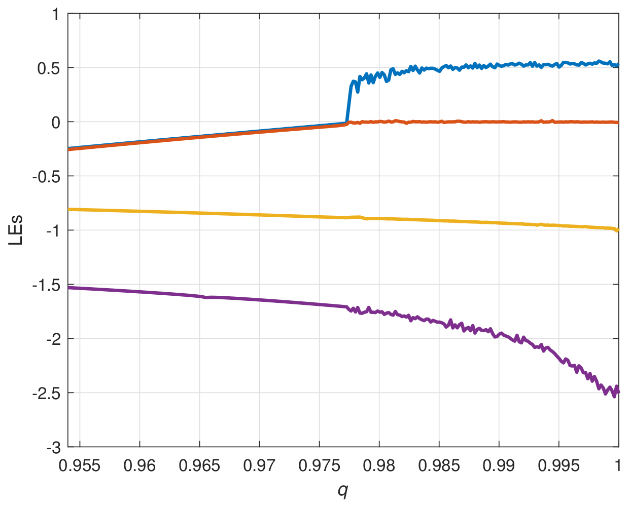
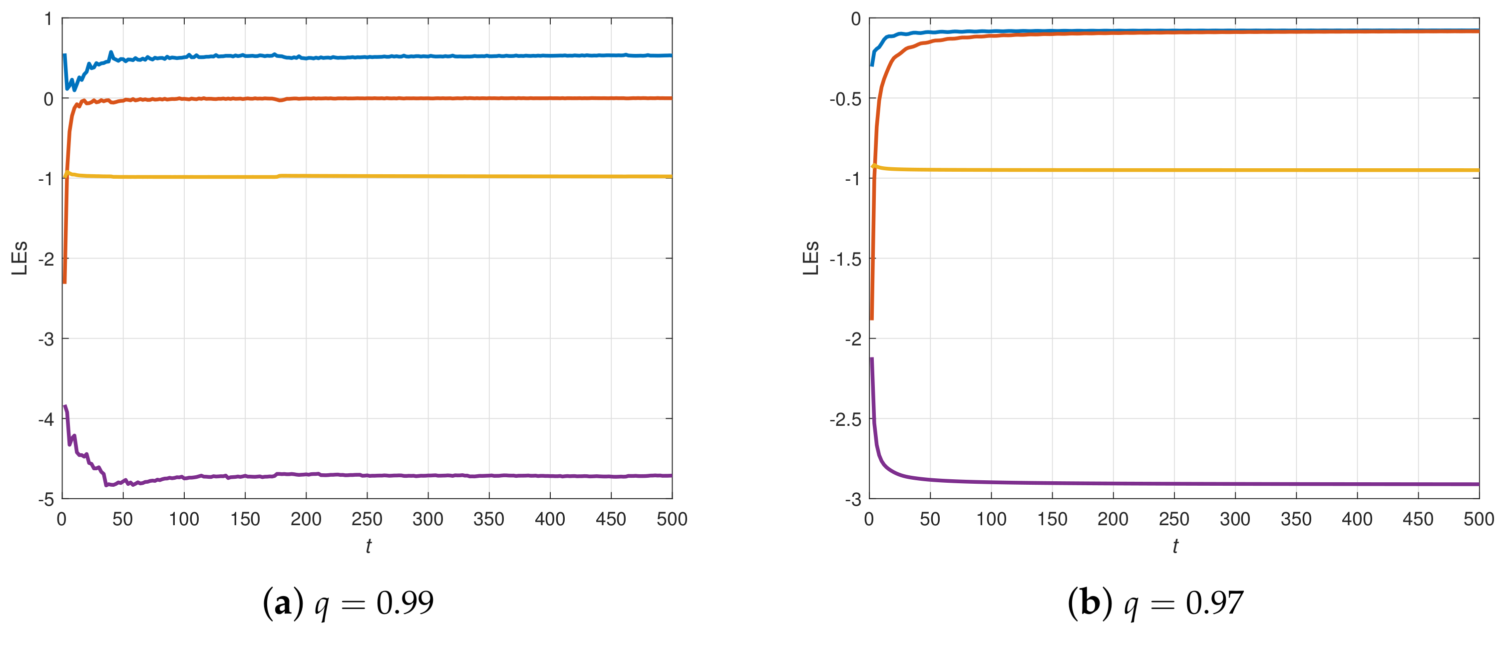
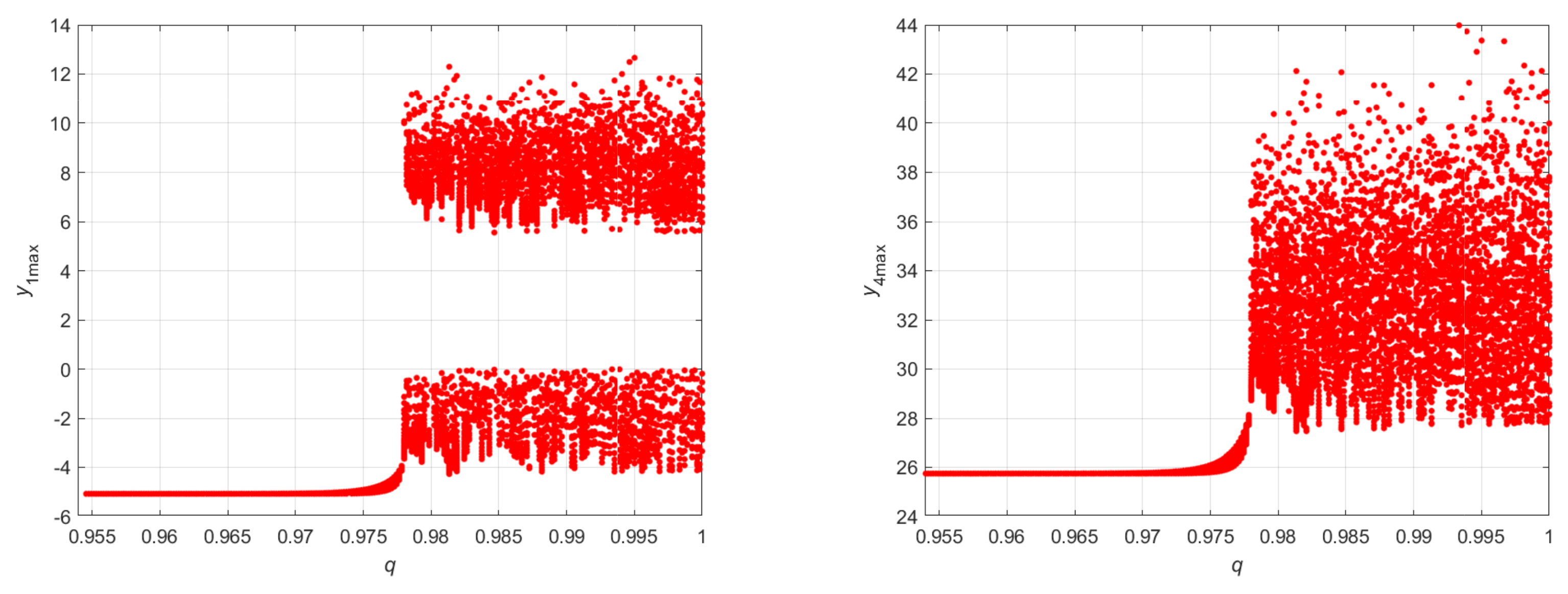
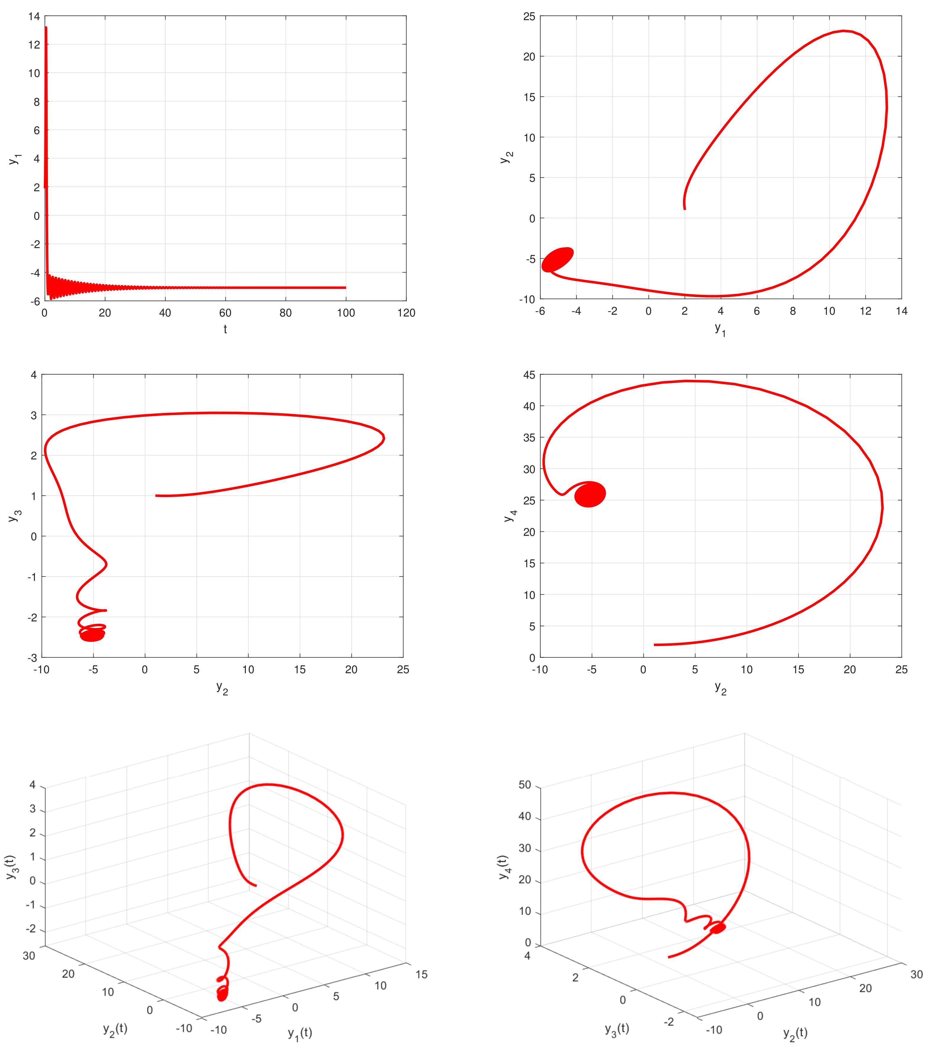
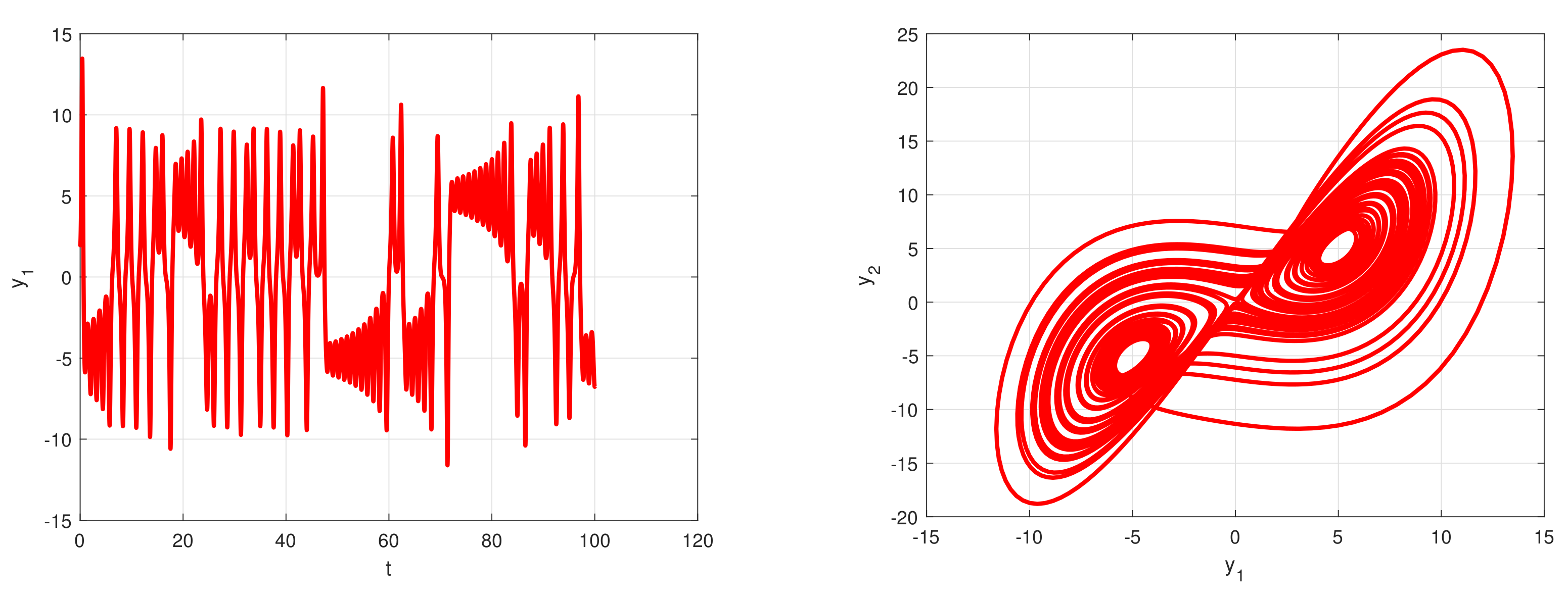
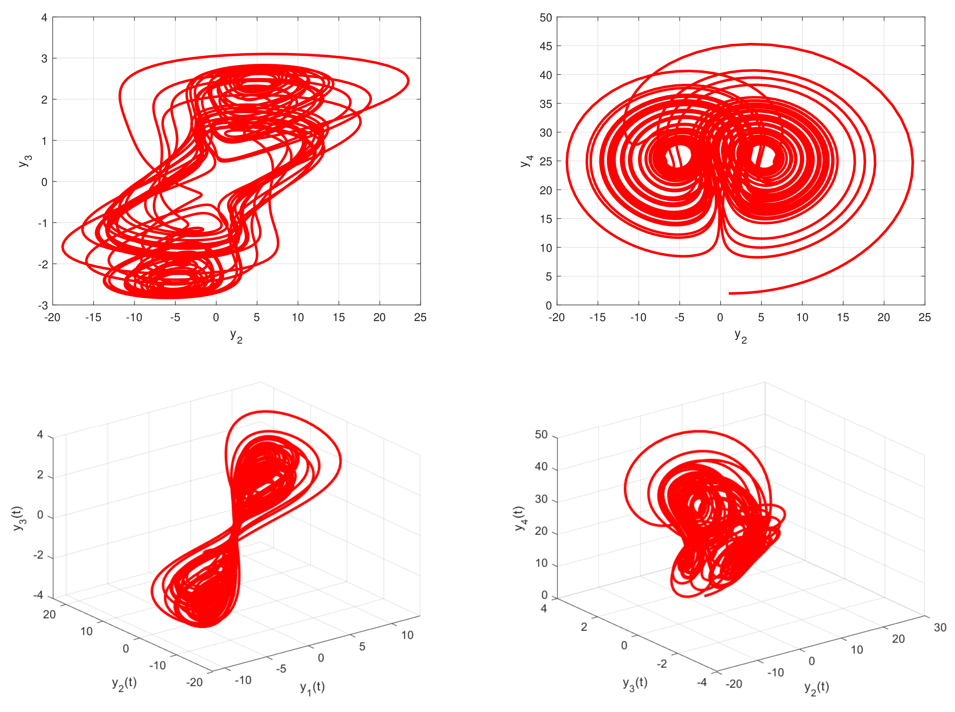
2.2. Dynamical Behaviors

In this section, the basic dynamical properties such as phase portraits, bifurcation diagram, Lyapunov exponents and chaos diagram of the fractional-order chaotic system (2) are presented.

Selecting the parameters $k=4,e=0.5,r=27,$ and $b=1$, Figure 1 depicts Lyapunov exponents. When $q=0.999,$ the values of Lyapunov exponents at 500th second are $L_1=0.5291$, $L_2=-0.0022$, $L_3=-0.9789$, and $L_4=-4.7122$.

The Benettin–Wolf algorithm to determine all Lyapunov exponents for the fractional-order systems modeled by Caputo’s derivative is used [35]. The values of Lyapunov exponents at 500th second are obtained as $L_1=-0.0783$, $L_2=-0.0839$, $L_3=-0.9501$, and $L_4=-2.9103$. As it is clear from Figure 1 and Figure 2, for some values of q, system (2) has positive Lyapunov exponent and therefore is in a chaotic state and for different values of q, system (2) converges to the equilibrium point.

The bifurcation diagram of system (2) is drawn based on the change of the derivative order parameter and by fixing the values of other parameters as $k=4,e=0.5,r=27,$ and $b=1$. Figure 3, shows the effect of varying parameter q in the interval $(0.954,1).$ It is obvious that with different values of the derivative order of q, the system (2) is in stable, periodic and chaotic state and the bifurcation diagram is well consistent with the Lyapunov exponent spectrum. The system is stable in $q\in (0.954,0.978)$ and the system exhibits chaotic behavior when $q\in (0.978,1)$.

When $k=4,e=0.5,r=27,$ and $b=1$, the phase portraits of system (2) are shown in Figure 4, that indicates for the value of $q=0.97,$ the trajectories of the system converge to the equilibrium point.

When $q=0.99,k=4,e=0.5,r=27,$ and $b=1$, the phase portraits of system (2) are shown in Figure 5. The system exhibits the chaotic behavior and the equilibrium point is not stable.

3. Chaos Control

In this section, we apply the linear feedback control method to stabilize system (2) to its equilibrium points. Let consider the following controlled form of fractional-order system (2):

$$\begin{array}{ccc}\hfill & & D_t^q{y}_1\left(t\right)=-k{y}_1+k{y}_2-w_1(y_1-y_1^{*}),\hfill \\ & & D_t^q{y}_2\left(t\right)=r{y}_1-y_2-e{y}_3-y_1{y}_4-w_2(y_2-y_2^{*}),\hfill \\ & & D_t^q{y}_3\left(t\right)=e{y}_2-y_3-w_3(y_3-y_3^{*}),\hfill \\ & & D_t^q{y}_4\left(t\right)=-b{y}_4+y_1{y}_2-w_4(y_4-y_4^{*}),\hfill \end{array}$$

(9)

where $w_1,w_2,w_3,w_4$ are control parameters and $E*$ is the equilibrium point of the system (2).

The Jacobian matrix at $E*$ for the system (9) is obtained as

$$J\left(E*\right)=\left[\begin{array}{cccc}-k-w_1& k& 0& 0\\ \\ r-y_4^{*}& -1-w_2& -e& -y_1^{*}\\ \\ 0& e& -1-w_3& 0\\ \\ y_2^{*}& y_1^{*}& 0& -b-w_4\end{array}\right].$$

The characteristic equation of the Jacobian matrix $J\left(E*\right)$ is given by

$$\begin{array}{ccc}& & f\left(\lambda \right)=\left|\begin{array}{cccc}\lambda +k+w_1& -k& 0& 0\\ \\ y_4^{*}-r& \lambda +1+w_2& e& y_1^{*}\\ \\ 0& -e& \lambda +1+w_3& 0\\ \\ -y_2^{*}& -y_1^{*}& 0& \lambda +b+w_4\end{array}\right|=0.\hfill \end{array}$$

Selecting $k_1=1,k_2=2,k_3=3$ and $k_4=4,$ the characteristic polynomial of for the equilibrium point $E_1$ with the parameters $k=4,e=0.5,r=27,$ and $b=1$ is given as

$$\begin{array}{c}\hfill C\left(\lambda \right)={\lambda }^4+17{\lambda }^3+128{\lambda }^2+587.25\lambda +1133.25=0,\end{array}$$

(10)

and the characteristic roots of Equation (10) are calculated as

$$\begin{array}{ccc}& & {\lambda }_1=-2.539703887-5.413874345i,{\lambda }_2=-7.918563161,\hfill \\ & & {\lambda }_3=-4.002029066, {\lambda }_4=-2.539703887+5.413874345i.\hfill \end{array}$$

Since, all the eigenvalues of Equation (10) are negative real numbers and complex numbers with negative real parts, therefore the equilibrium point $E_1$ is asymptotically stable for all $0<q<1$. When $q=0.99,k=4,e=0.5,r=27,$ and $b=1$, the phase portraits and time series of the controlled system (9) are shown in Figure 6.

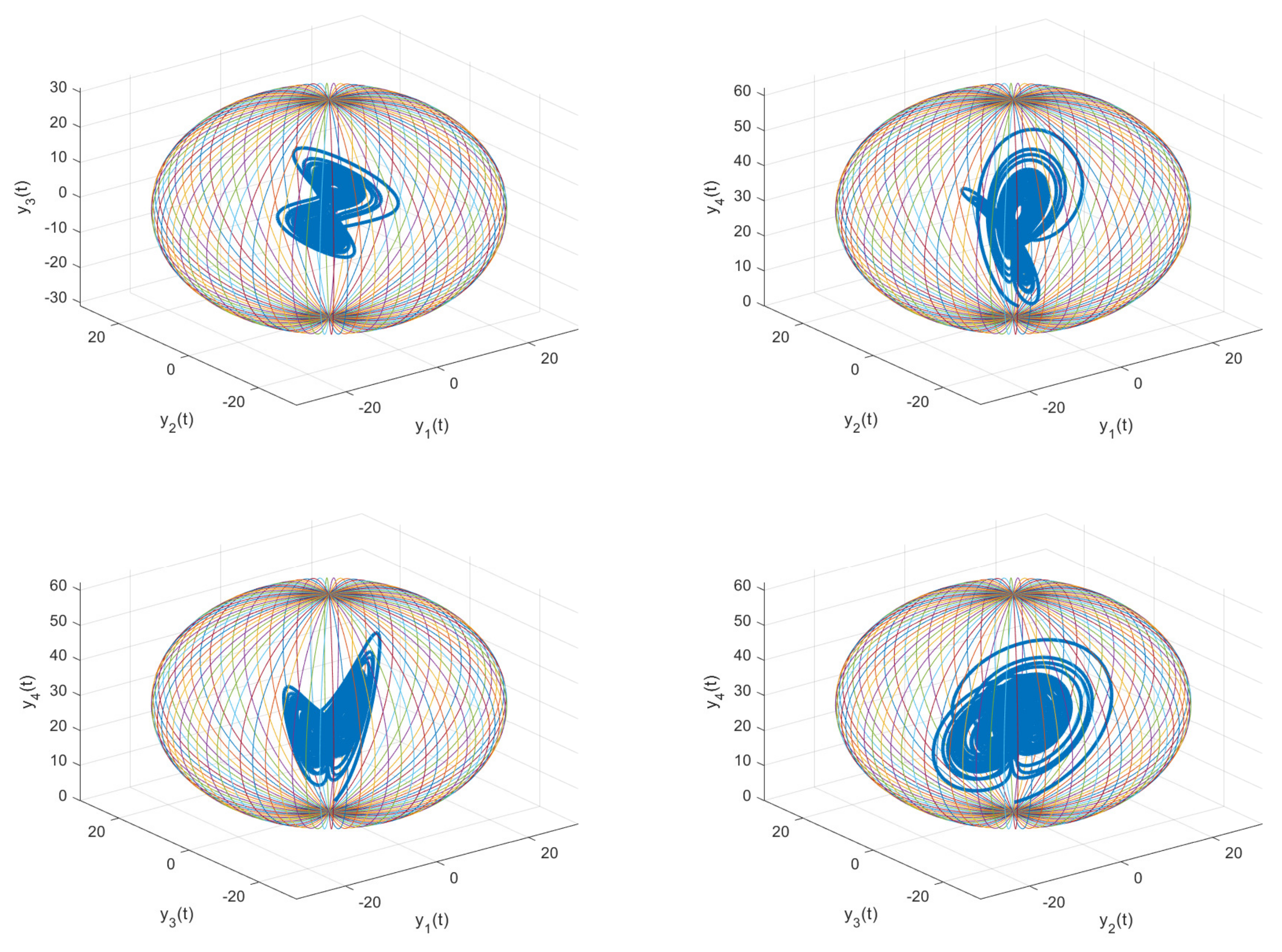
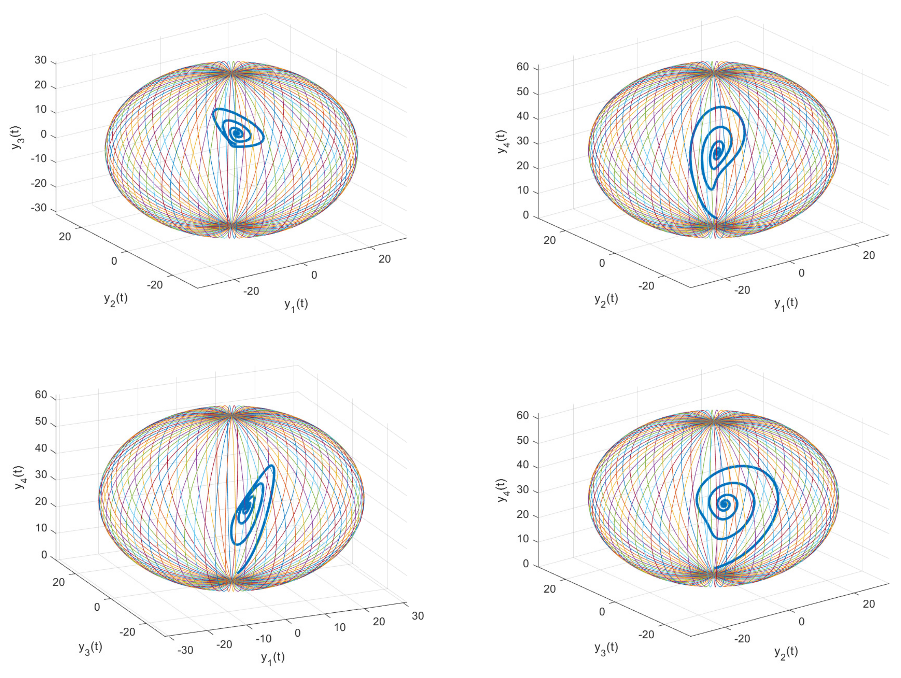
4. Global Mittag–Leffler Attractive Sets

In this section, our main aim is to estimate the global Mittag–Leffler attractive sets (MLASs) and Mittag–Leffler positive invariant sets (MLPISs) for the fractional-order chaotic system (2). Firstly, we introduce some definitions for calculating the MLAS and MLPIS of fractional-order systems with only cross-product nonlinearities.

Lemma 1

([32]). Let $y\left(t\right)\in \mathbb{R},$ is the continuous and differentiable functions, then

$$\begin{array}{c}\hfill \frac{1}{2}{D}^q\left(y^2\left(t\right)\right)\le y\left(t\right)D^q\left(y\right(t\left)\right),\end{array}$$

(11)

Lemma 2

([32]). For $q\in (0,1)$ and constant $\gamma \in \mathbb{R}$, if a continuous function $y\left(t\right)$ meets

$$\begin{array}{c}\hfill D^q\left(y\right(t\left)\right)\le \gamma y\left(t\right),t\ge 0,\end{array}$$

(12)

then

$$\begin{array}{c}\hfill y\left(t\right)\le y\left(0\right)E_q\left(\gamma t^q\right),t\ge 0.\end{array}$$

(13)

Definition 2

([32]). Let us consider the following fractional-order system

$$\begin{array}{c}\hfill D_t^q{y}_i=f\left(y_i\right),y_i\left(t_0\right)=y_{i,0},i=1,2,\cdots ,n,\end{array}$$

(14)

where $y_i\in {\mathbb{R}}^n$, $f:{\mathbb{R}}^n\to {\mathbb{R}}^n$ is sufficiently smooth, and $y_i(t,t_0,y_{i,0})$ is the solution.

For a given Lyapunov function $\mathcal{L}\left(Y\right(t\left)\right)$, if there exist constants ${\mathcal{K}}_{\gamma }>0$ and $\gamma >0 for all$$Y_0\in {\mathbb{R}}^n$ such that

$$\begin{array}{c}\hfill \mathcal{L}\left(Y\left(t\right)\right)-{\mathcal{K}}_{\gamma }\le (\mathcal{L}\left(Y\left(t_0\right)\right)-{\mathcal{K}}_{\gamma })E_q\left(-\gamma {(t-t_0)}^q\right),t\ge t_0,\end{array}$$

(15)

for $\mathcal{L}\left(Y\left(t\right)\right)>{\mathcal{K}}_{\gamma }$, then $\mathcal{G}=\left\{(y_1,y_2,\cdots ,y_n)\right|\mathcal{L}\left(Y\left(t\right)\right)\le {\mathcal{K}}_{\gamma }\}$ is said to be the global Mittag–Leffler attractive sets (MLASs) of system (14). If for any $Y_0\in \mathcal{G}$ and any $t>t_0,Y(t,t_0,Y_0)\in \mathcal{G}$, then $\mathcal{G}$ is said to be a Mittag–Leffler positive invariant sets (MLPISs).

4.1. Main Results

Here we will discuss the ultimate bound of a class of the fractional-order chaotic systems with only cross-product nonlinearities:

$$D_t^q{y}_1\left(t\right)=\sum _{j=1}^4{\alpha }_{1j}{y}_j+\sum _{j=1}^4\sum _{k=1}^4{\beta }_{1jk}{y}_j{y}_k+r_1,$$

$$D_t^q{y}_2\left(t\right)=\sum _{j=1}^4{\alpha }_{2j}{y}_j+\sum _{j=1}^4\sum _{k=1}^4{\beta }_{2jk}{y}_j{y}_k+r_2,$$

(16)

$$D_t^q{y}_3\left(t\right)=\sum _{j=1}^4{\alpha }_{3j}{y}_j+\sum _{j=1}^4\sum _{k=1}^4{\beta }_{3jk}{y}_j{y}_k+r_3,$$

$$D_t^q{y}_4\left(t\right)=\sum _{j=1}^4{\alpha }_{4j}{y}_j+\sum _{j=1}^4\sum _{k=1}^4{\beta }_{4jk}{y}_j{y}_k+r_4.$$

(17)

The candidate Lyapunov function for this problem is defined as follows

$$\begin{array}{c}\hfill \mathcal{L}\left(Y\left(t\right)\right)=\frac{1}{2}{({\omega }_1{y}_1-s_1)}^2+\frac{1}{2}{({\omega }_2{y}_2-s_2)}^2+\frac{1}{2}{({\omega }_3{y}_3-s_3)}^2+\frac{1}{2}{({\omega }_4{y}_4-s_4)}^2,\end{array}$$

(18)

where ${\omega }_i,s_i,i=1,2,3,4$ are known parameters. The function $h(Y,\delta )$ is considered as follows

$$\begin{array}{ccc}\hfill & & h(Y,\delta )={\omega }_1({\omega }_1{y}_1-s_1)\left(\sum _{j=1}^4{\alpha }_{1j}{y}_j+\frac{{\delta }_1}{{\omega }_1}({\omega }_1{y}_1-s_1)+\sum _{j=1}^4\sum _{k=1}^4{\beta }_{1jk}{y}_j{y}_k+r_1\right)\hfill \\ & & +{\omega }_2({\omega }_2{y}_2-s_2)\left(\sum _{j=1}^4{\alpha }_{2j}{y}_j+\frac{{\delta }_2}{{\omega }_2}({\omega }_2{y}_2-s_2)+\sum _{j=1}^4\sum _{k=1}^4{\beta }_{2jk}{y}_j{y}_k+r_2\right)\hfill \\ & & +{\omega }_3({\omega }_3{y}_3-s_3)\left(\sum _{j=1}^4{\alpha }_{3j}{y}_j+\frac{{\delta }_3}{{\omega }_3}({\omega }_3{y}_3-s_3)+\sum _{j=1}^4\sum _{k=1}^4{\beta }_{3jk}{y}_j{y}_k+r_3\right)\hfill \\ & & +{\omega }_4({\omega }_4{y}_4-s_4)\left(\sum _{j=1}^4{\alpha }_{4j}{y}_j+\frac{{\delta }_4}{{\omega }_4}({\omega }_4{y}_4-s_4)+\sum _{j=1}^4\sum _{k=1}^4{\beta }_{4jk}{y}_j{y}_k+r_4\right),\hfill \end{array}$$

(19)

where $\delta =({\delta }_1,{\delta }_2,{\delta }_3,{\delta }_4)$.

Theorem 2.

Let $h(Y_0,\delta )>0$ is the supremum of function $h(Y,\delta )$ on $Y\in {\mathbb{R}}^4$ defined in (19), $\gamma =min\{{\delta }_1,{\delta }_2,{\delta }_3,{\delta }_4\}.$ Then the following inequality is fulfilled:

$$\begin{array}{c}\hfill \mathcal{L}\left(Y\left(t\right)\right)-\frac{1}{2\gamma }h(Y_0,\delta )\le \left(\mathcal{L}\left(Y\left(t_0\right)\right)-\frac{1}{2\gamma }h(Y_0,\delta )\right)E_q\left(-2\gamma {(t-t_0)}^q\right),t\ge t_0.\end{array}$$

(20)

Furthermore,

$$\begin{array}{ccc}\hfill & & \mathcal{G}=\{Y|\mathcal{L}\left(Y\left(t\right)\right)\le \frac{1}{2\gamma }h(Y_0,\delta )\}\hfill \\ & & =\{Y|{({\omega }_1{y}_1-s_1)}^2+{({\omega }_2{y}_2-s_2)}^2+{({\omega }_3{y}_3-s_3)}^2+{({\omega }_4{y}_4-s_4)}^2\le \frac{1}{\gamma }h(Y_0,\delta )\},\hfill \end{array}$$

(21)

is the Mittag–Leffler attractive sets (MLASs) and Mittag–Leffler positive invariant sets (MLPISs) of system (2).

Proof. 

Computing the fractional derivative of $\mathcal{L}\left(Y\right(t\left)\right)$ along the trajectory of system (16) and using Lemma 1, we have

$$\begin{array}{ccc}& & D^q\mathcal{L}\left(Y\left(t\right)\right)\le ({\omega }_1{y}_1-s_1)D^q{\omega }_1{y}_1+({\omega }_2{y}_2-s_2)D^q{\omega }_2{y}_2+({\omega }_3{y}_3-s_3)D^q{\omega }_3{y}_3\hfill \\ & & +({\omega }_4{y}_4-s_4)D^q{\omega }_4{y}_4\hfill \\ & & ={\omega }_1({\omega }_1{y}_1-s_1)\left(\sum _{j=1}^4{\alpha }_{1j}{y}_j+\sum _{j=1}^4\sum _{k=1}^4{\beta }_{1jk}{y}_j{y}_k+r_1\right)\hfill \\ & & +{\omega }_2({\omega }_2{y}_2-s_2)\left(\sum _{j=1}^4{\alpha }_{2j}{y}_j+\sum _{j=1}^4\sum _{k=1}^4{\beta }_{2jk}{y}_j{y}_k+r_2\right)\hfill \\ & & +{\omega }_3({\omega }_3{y}_3-s_3)\left(\sum _{j=1}^4{\alpha }_{3j}{y}_j+\sum _{j=1}^4\sum _{k=1}^4{\beta }_{3jk}{y}_j{y}_k+r_3\right)\hfill \end{array}$$

$$\begin{array}{ccc}\hfill & & +{\omega }_4({\omega }_4{y}_4-s_4)\left(\sum _{j=1}^4{\alpha }_{4j}{y}_j+\sum _{j=1}^4\sum _{k=1}^4{\beta }_{4jk}{y}_j{y}_k+r_4\right)\hfill \\ & & =-{\delta }_1{({\omega }_1{y}_1-s_1)}^2-{\delta }_2{({\omega }_2{y}_2-s_2)}^2-{\delta }_3{({\omega }_3{y}_3-s_3)}^2-{\delta }_4{({\omega }_4{y}_4-s_4)}^2\hfill \\ & & +h(Y,\delta )\le -\gamma \sum _{j=1}^4{({\omega }_j{y}_j-s_j)}^2+h(Y,\delta )\hfill \\ & & \le -\gamma \sum _{j=1}^4{({\omega }_j{y}_j-s_j)}^2+h(Y_0,\delta ).\hfill \end{array}$$

(22)

From there we have

$$\begin{array}{c}\hfill D^q\mathcal{L}\left(Y\left(t\right)\right)\le -2\gamma \mathcal{L}\left(Y\left(t\right)\right)+h(Y_0,\delta ),\end{array}$$

(23)

i.e.,

$$\begin{array}{c}\hfill D^q\left(\mathcal{L}\left(Y\left(t\right)\right)-\frac{1}{2\gamma }h(Y_0,\delta )\right)\le -2\gamma \left[\mathcal{L}\left(Y\left(t\right)\right)-\frac{1}{2\gamma }h(Y_0,\delta )\right].\end{array}$$

(24)

According to Lemma 2, we obtain

$$\begin{array}{c}\hfill \mathcal{L}\left(Y\left(t\right)\right)-\frac{1}{2\gamma }h(Y_0,\delta )\le (\mathcal{L}\left(Y_0\right)-\frac{1}{2\gamma }h(Y_0,\delta ))E_q(-2\gamma t^q),t\ge 0.\end{array}$$

(25)

Finally, Definition 2, indicates that the ellipsoid $\mathcal{G}$ is the Mittag–Leffler attractive sets (MLASs) and Mittag–Leffler positive invariant sets (MLPISs) of the system (2). □

4.2. MLAS and MLPIS for the Fractional-Order System (2)

To investigate the correctness of Theorem 4.1, we consider the calculation of the bound set for the fractional-order system (2). The following theorem determines the necessary conditions for estimating the MLAS and MLPIS for the system (2).

Theorem 3. 

Let consider ${\delta }_1<k,{\delta }_2<1,{\delta }_3<1,{\delta }_4<b,$ and $E_0=(y_1^0,y_2^0,y_3^0,y_4^0)$ be the stable point of $h(Y,\delta )$ defined by (19). Moreover, the Hessian Matrix of $h(Y,\delta )$ is a negative definite matrix on $E_0$. Then,

$$\begin{array}{c}\hfill \mathcal{G}=\left\{Y\left(t\right)\in {\mathbb{R}}^4\mid {\omega }_1{y}_1^2+{\omega }_2{y}_2^2+{\omega }_3{y}_3^2+{\omega }_2{(y_4-\frac{k{\omega }_1+r{\omega }_2}{{\omega }_2})}^2\le \frac{b^2{(k{\omega }_1+r{\omega }_2)}^2}{4\gamma (b-{\delta }_4)}\right\},\end{array}$$

(26)

is the Mittag–Leffler attractive sets (MLASs) and Mittag–Leffler positive invariant sets (MLPISs) of the system (2).

Proof. 

Let ${\alpha }_{11}=-k,{\alpha }_{12}=k,{\alpha }_{21}=r,{\alpha }_{22}=-1,{\alpha }_{23}=-e,{\alpha }_{32}=e,{\alpha }_{33}=-1$, ${\alpha }_{44}=-b,{\beta }_{214}=-1,{\beta }_{412}=1,r_1=r_2=r_3=r_4=0,$ else ${\alpha }_{ij}=0,{\beta }_{ijk}=0,$ and $s_1=s_2=s_3=0,s_4=k{\omega }_1+r{\omega }_2.$

Thus, $\mathcal{L}\left(Y\right(t\left)\right)$ can be rewritten as:

$$\begin{array}{c}\hfill \mathcal{L}\left(Y\left(t\right)\right)=\frac{1}{2}{\omega }_1{y}_1^2+\frac{1}{2}{\omega }_2{y}_2^2+\frac{1}{2}{\omega }_3{y}_3^2+\frac{1}{2}{\omega }_2{(y_4-\frac{k{\omega }_1+r{\omega }_2}{{\omega }_2})}^2,\end{array}$$

(27)

and

$$\begin{array}{ccc}\hfill & & h(Y,\delta )={\omega }_1^2{y}_1\left(-k{y}_1+k{y}_2+{\delta }_1{y}_1\right)+{\omega }_2^2{y}_2\left(r{y}_1-y_2-e{y}_3-y_1{y}_4+{\delta }_2{y}_2\right)\hfill \\ & & +{\omega }_3^2{y}_3\left(e{y}_2-y_3+{\delta }_3{y}_3\right)+{\omega }_2\left({\omega }_2{y}_4-(k{\omega }_1+r{\omega }_2)\right)\hfill \\ & & (-b{y}_4+y_1{y}_2+\frac{{\delta }_4}{{\omega }_2}({\omega }_2{y}_4-(k{\omega }_1+r{\omega }_2))).\hfill \end{array}$$

Since $E_0$ is the stable point of the $h(Y,\delta )$, we have

$$\begin{array}{c}\hfill \nabla {\left(h\right)}_{E_0}=(h_{y_1}^{\prime },h_{y_2}^{\prime },h_{y_3}^{\prime },h_{y_4}^{\prime })=0.\end{array}$$

(28)

and the Hessian Matrix H of the $h(Y,\delta )$ is a negative definite matrix. Therefore,

$$\begin{array}{ccc}\hfill & & h_{y_1}^{\prime }={\omega }_1^2(-k{y}_1+k{y}_2+{\delta }_1{y}_1)+{\omega }_1^2{y}_1(-k+{\delta }_1)+{\omega }_2^2{y}_2(r-y_4)\hfill \\ & & +{\omega }_2(-k{\omega }_1-r{\omega }_2+{\omega }_2{y}_4)y_2,\hfill \\ & & \\ & & h_{y_2}^{\prime }={\omega }_1^2{y}_{1}k+{\omega }_2^2(-e{y}_3+r{y}_1+{\delta }_2{y}_2-y_1{y}_4-y_2)+{\omega }_2^2{y}_2({\delta }_2-1)+{\omega }_3^2{y}_{3}e\hfill \\ & & +{\omega }_2(-k{\omega }_1-r{\omega }_2+{\omega }_2{y}_4)y_1,\hfill \\ & & \\ & & h_{y_3}^{\prime }=-{\omega }_2^2{y}_{2}e+{\omega }_3^2(e{y}_2+{\delta }_3{y}_3-y_3)+{\omega }_3^2{y}_3({\delta }_3-1),\hfill \\ & & \\ & & h_{y_4}^{\prime }=-{\omega }_2^2{y}_2{y}_1+{\omega }_2^2(-b{y}_4+y_1{y}_2+{\delta }_4(-k{\omega }_1-r{\omega }_2+{\omega }_2{y}_4)/{\omega }_2)\hfill \\ & & +{\omega }_2(-k{\omega }_1-r{\omega }_2+{\omega }_2{y}_4)(-b+{\delta }_4),\hfill \\ & & h_{y_1{y}_1}^{\prime \prime }=2{\omega }_1^2(-k+{\delta }_1),\hfill \\ & & h_{y_2{y}_2}^{\prime \prime }=2{\omega }_2^2({\delta }_2-1),\hfill \\ & & h_{y_3{y}_3}^{\prime \prime }=2{\omega }_3^2({\delta }_3-1),\hfill \\ & & h_{y_4{y}_4}^{\prime \prime }=2{\omega }_2^2(-b+{\delta }_4),\hfill \\ & & h_{y_1{y}_2}^{\prime \prime }=h_{y_2{y}_1}^{\prime \prime }=k{\omega }_1^2-k{\omega }_1{\omega }_2,\hfill \end{array}$$

$$\begin{array}{ccc}& & h_{y_1{y}_3}^{\prime \prime }=h_{y_3{y}_1}^{\prime \prime }=0,\hfill \\ & & h_{y_1{y}_4}^{\prime \prime }=h_{y_4{y}_1}^{\prime \prime }=0,\hfill \\ & & h_{y_2{y}_3}^{\prime \prime }=h_{y_3{y}_2}^{\prime \prime }=-e{\omega }_2^2+e{\omega }_3^2,\hfill \\ & & h_{y_2{y}_4}^{\prime \prime }=h_{y_4{y}_2}^{\prime \prime }=0,\hfill \\ & & h_{y_3{y}_4}^{\prime \prime }=h_{4y_3}^{\prime \prime }=0,\hfill \end{array}$$

$$\left|\begin{array}{cc}{h}_{y_1{y}_1}^{″}& h_{y_1{y}_2}^{″}\\ \\ h_{y_2{y}_1}^{″}& h_{y_2{y}_2}^{″}\end{array}\right|=\left|\begin{array}{cc}2{\omega }_1^2(-k+{\delta }_1)& k{\omega }_1^2-k{\omega }_1{\omega }_2\\ \\ k{\omega }_1^2-k{\omega }_1{\omega }_2& 2{\omega }_2^2({\delta }_2-1)\end{array}\right|>0,$$

$$\left|\begin{array}{ccc}{h}_{y_1{y}_1}^{″}& h_{y_1{y}_2}^{″}& h_{y_1{y}_3}^{″}\\ \\ h_{y_2{y}_1}^{″}& h_{y_2{y}_2}^{″}& h_{y_2{y}_3}^{″}\\ \\ h_{y_3{y}_1}^{″}& h_{y_3{y}_2}^{″}& h_{y_3{y}_3}^{″}\end{array}\right|=\left|\begin{array}{ccc}2{\omega }_1^2(-k+{\delta }_1)& k{\omega }_1^2-k{\omega }_1{\omega }_2& 0\\ \\ k{\omega }_1^2-k{\omega }_1{\omega }_2& 2{\omega }_2^2({\delta }_2-1)& -e{\omega }_2^2+e{\omega }_3^2\\ \\ 0& -e{\omega }_2^2+e{\omega }_3^2& 2{\omega }_3^2({\delta }_3-1)\end{array}\right|<0.$$

And

$$\left|\begin{array}{cccc}{h}_{y_1{y}_1}^{″}& h_{y_1{y}_2}^{″}& h_{y_1{y}_3}^{″}& h_{y_1{y}_4}^{″}\\ \\ h_{y_2{y}_1}^{″}& h_{y_2{y}_2}^{″}& h_{y_2{y}_3}^{″}& h_{y_2{y}_4}^{″}\\ \\ h_{y_3{y}_1}^{″}& h_{y_3{y}_2}^{″}& h_{y_3{y}_3}^{″}& h_{y_3{y}_4}^{″}\\ \\ h_{y_4{y}_1}^{″}& h_{y_4{y}_2}^{″}& h_{y_4{y}_3}^{″}& h_{y_4{y}_4}^{″}\end{array}\right|=\left|\begin{array}{cccc}2{\omega }_1^2(-k+{\delta }_1)& k{\omega }_1^2-k{\omega }_1{\omega }_2& 0& 0\\ \\ k{\omega }_1^2-k{\omega }_1{\omega }_2& 2{\omega }_2^2({\delta }_2-1)& -e{\omega }_2^2+e{\omega }_3^2& 0\\ \\ 0& -e{\omega }_2^2+e{\omega }_3^2& 2{\omega }_3^2({\delta }_3-1)& 0\\ \\ 0& 0& 0& 2{\omega }_2^2(-b+{\delta }_4)\end{array}\right|>0.$$

By solving the following system we will have

$$\begin{array}{c}\hfill \left\{\begin{array}{c}{h}_{y_1}^{\prime }=0,\hfill \\ h_{y_2}^{\prime }=0,\hfill \\ h_{y_3}^{\prime }=0,\hfill \\ h_{y_4}^{\prime }=0.\hfill \end{array}\right.\end{array}$$

(29)

$y_1=y_2=y_3=0,y_4=\frac{(b-2{\delta }_4)(k{\omega }_1+r{\omega }_2)}{2{\omega }_2(b-{\delta }_4)},$ and ${\displaystyle h(Y,\delta )\le \underset{Y\in {\mathbb{R}}^4}{sup}h(Y,\delta )=\frac{b^2{(k{\omega }_1+r{\omega }_2)}^2}{4(b-{\delta }_4)}.}$

Using Lemma 2, gives the following result

$$\begin{array}{c}\hfill \mathcal{L}\left(Y\left(t\right)\right)-\frac{b^2{(k{\omega }_1+r{\omega }_2)}^2}{8\gamma (b-{\delta }_4)}\le \left[\mathcal{L}\left(Y\left(0\right)\right)-\frac{b^2{(k{\omega }_1+r{\omega }_2)}^2}{8\gamma (b-{\delta }_4)}\right]E_q(-2\gamma t^q),t\ge 0.\end{array}$$

and the Mittag–Leffler attractive sets (MLASs) and Mittag–Leffler positive invariant sets (MLPISs) of the system (2) is

$$\begin{array}{c}\hfill \mathcal{G}=\left\{Y\left(t\right)\in {\mathbb{R}}^4\mid {\omega }_1{y}_1^2+{\omega }_2{y}_2^2+{\omega }_3{y}_3^2+{\omega }_2{(y_4-\frac{k{\omega }_1+r{\omega }_2}{{\omega }_2})}^2\le \frac{b^2{(k{\omega }_1+r{\omega }_2)}^2}{4\gamma (b-{\delta }_4)}\right\},\end{array}$$

(30)

□

Remark 1.

It is obvious that by changing the parameters ${\omega }_1,{\omega }_2,{\omega }_3,{\delta }_1,{\delta }_2,{\delta }_3,$ and ${\delta }_4$, different estimates of the global attractive set and the positive reliable set for system (2) can be obtained.

Let us take ${\omega }_1={\omega }_2={\omega }_3=1,{\delta }_1=1,{\delta }_2={\delta }_3={\delta }_4=0.999,$ $q=0.99,k=4$, $e=0.5,r=27,$ and $b=1.$ Then

$$\begin{array}{c}\hfill \mathcal{G}=\left\{(y_1,y_2,y_3,y_4)|y_1^2+y_2^2+y_3^2+{(y_4-31)}^2\le {\left(31\right)}^2\right\}.\end{array}$$

is the Mittag–Leffler MLAS and Mittag–Leffler MLPIS of system (2). Figure 7 shows the Mittag–Leffler MLAS and phase portrait of system (2).

When $q=0.9,k=4,e=0.5,r=27,$ and $b=1,$ Figure 8 shows the phase portrait and Mittag–Leffler MLAS of system (2).

5. Conclusions

In this paper, we present a four-dimensional fractional-order system with cross-product nonlinearities. Using the concept of stability in fractional-order systems, the stability of equilibrium points and chaos control were performed theoretically and numerically. Furthermore, the dynamical characteristics of the considered system, such as the existence or absence of chaos, bifurcation diagrams, and Lyapunov exponents are investigated. Finally, the estimation of the MLASs and MLPISs for a fractional system that belongs to a special class of nonlinear systems is presented.

References

1. Hilfer, R. Applications of Fractional Calculus in Physics; World Scientific: Singapore, 2000. [Google Scholar]
2. Tavazoei, M.S.; Haeri, M. Synchronization of chaotic fractional-order systems via active sliding mode controller. Physica A 2008, 387, 57–70. [Google Scholar] [CrossRef]
3. He, Y.; Peng, J.; Zheng, S. Fractional-order financial system and fixed-time synchronization. Fractal Fract. 2022, 6, 507. [Google Scholar] [CrossRef]
4. Ahmed, E.; El-Sayed, A.M.A.; El-Saka, H.A.A. On some Routh-Hurwitz conditions for fractional order differential equations and their applications in Lorenz, Rössler, Chua and Chen systems. Phys. Lett. A 2006, 358, 1–4. [Google Scholar] [CrossRef]
5. He, Y.; Zheng, S.; Yuan, L. Dynamics of fractional-order digital manufacturing supply chain system and its control and synchronization. Fractal Fract. 2021, 5, 128. [Google Scholar] [CrossRef]
6. Zhou, P.; Ma, J.; Tang, J. Clarify the physical process for fractional dynamical systems. Nonlinear Dyn. 2020, 100, 2353–2364. [Google Scholar] [CrossRef]
7. Aghababa, M.P. Comments on “H synchronization of uncertain fractional order chaotic systems: Adaptive fuzzy approach” [ISA Trans 50, 548–556 (2011)]. ISA Trans. 2012, 51, 11–12. [Google Scholar] [CrossRef]
8. Chen, Y.; Wang, B.; Chen, Y.; Wang, Y. Sliding mode control for a class of nonlinear fractional order systems with a fractional fixed-time reaching law. Fractal Fract. 2022, 6, 678. [Google Scholar] [CrossRef]
9. Mahmoud, G.M.; Arafa, A.A.; Abed-Elhameed, T.M.; Mahmoud, E.E. Chaos control of integer and fractional orders of chaotic Burke–Shaw system using time delayed feedback control. Chaos Solitons Fractals 2017, 104, 680–692. [Google Scholar] [CrossRef]
10. Pham, V.T.; Kingni, S.T.; Volos, C.; Jafari, S.; Kapitaniak, T. A simple three-dimensional fractional-order chaotic system without equilibrium: Dynamics, circuitry implementation, chaos control and synchronization. Int. J. Electron. Commun. 2017, 78, 220–227. [Google Scholar] [CrossRef]
11. Wang, S.; He, S.; Yousefpour, A.; Jahanshahi, H.; Repnik, R.; Perc, M. Chaos and complexity in a fractional-order financial system with time delays. Chaos Solitons Fractals 2020, 131, 109521. [Google Scholar] [CrossRef]
12. Sayed, W.S.; Roshdy, M.; Said, L.A.; Herencsar, N.; Radwan, A.G. CORDIC-based FPGA realization of a spatially rotating translational fractional-order multi-scroll grid chaotic system. Fractal Fract. 2022, 6, 432. [Google Scholar] [CrossRef]
13. Qi, F.; Qu, J.; Chai, Y.; Chen, L.; Lopes, A.M. Synchronization of incommensurate frractional-order chaotic systems based on linear feedback control. Fractal Fract. 2022, 6, 221. [Google Scholar] [CrossRef]
14. Gao, W.; Yan, L.; Saeedi, M.H.; Saberi Nik, H. Ultimate bound estimation set and chaos synchronization for a financial risk system. Math. Comput. Simul. 2018, 154, 19–33. [Google Scholar] [CrossRef]
15. Lin, Z.; Wang, H. Modeling and application of fractional-order economic growth model with time delay. Fractal Fract. 2021, 5, 74. [Google Scholar] [CrossRef]
16. Wen, C.; Yang, J. Complexity evolution of chaotic financial systems based on fractional calculus. Chaos Solitons Fractals 2019, 128, 242–251. [Google Scholar] [CrossRef]
17. Kuznetsov, N.; Leonov, G. Hidden attractors in dynamical systems: Systems with no equilibria, multistability and coexisting attractors. IFAC Proc. 2014, 47, 5445–5454. [Google Scholar] [CrossRef] [Green Version]
18. Leonov, G.; Kuznetsov, N. Hidden attractors in dynamical systems. From hidden oscillations in Hilbert-Kolmogorov, Aizerman, and Kalman problems to hidden chaotic attractor in Chua circuits. Int. J. Bifurc. Chaos 2013, 23, 1330002. [Google Scholar] [CrossRef] [Green Version]
19. Ouannas, A.; Khennaoui, A.A.; Momani, S.; Pham, V.T.; El-Khazali, R. Hidden attractors in a new fractional-order discrete system: Chaos, complexity, entropy, and control. Chin. Phys. B 2022, 29, 050504. [Google Scholar] [CrossRef]
20. Leonov, G.; Bunin, A.; Koksch, N. Attractor localization of the Lorenz system. Z. Angew. Math. Mech. 1987, 67, 649–656. [Google Scholar] [CrossRef]
21. Liao, X.; Fu, Y.; Xie, S. On the new results of global attractive set and positive invariant set of the Lorenz chaotic system and the applications to chaos control and synchronization. Sci. China Ser. F-Inf. Sci. 2005, 48, 304–321. [Google Scholar] [CrossRef]
22. Li, D.; Lu, J.A.; Wu, X.; Chen, G. Estimating the bounds for the Lorenz family of chaotic systems. Chaos Solitons Fractals 2005, 23, 529–534. [Google Scholar] [CrossRef]
23. Zhao, X.; Jiang, F.; Hu, J. Globally exponentially attractive sets and positive invariant sets of three-dimensional autonomous systems with only cross-product nonlinearities. Int. J. Bifurc. Chaos 2013, 23, 1350007. [Google Scholar] [CrossRef]
24. Kumar, D.; Kumar, S. Ultimate numerical bound estimation of chaotic dynamical finance model. In Modern Mathematical Methods and High Performance Computing in Science and Technology; Springer: Singapore, 2016; pp. 71–81. [Google Scholar]
25. Chien, F.; Chowdhury, A.R.; Saberi-Nik, H. Competitive modes and estimation of ultimate bound sets for a chaotic dynamical financial system. Nonlinear Dyn. 2021, 106, 3601–3614. [Google Scholar] [CrossRef]
26. Wang, H.; Dong, G. New dynamics coined in a 4-D quadratic autonomous hyper-chaotic system. Appl. Math. Comput. 2019, 346, 272–286. [Google Scholar] [CrossRef]
27. Chien, F.; Inc, M.; Yosefzade, H.R.; Saberi Nik, H. Predicting the chaos and solution bounds in a complex dynamical system. Chaos Solitons Fractals 2021, 153, 111474. [Google Scholar] [CrossRef]
28. Zhang, F.; Liao, X.; Chen, Y.A. On the dynamics of the chaotic general Lorenz system. Int. J. Bifurc. Chaos. 2017, 27, 1750075. [Google Scholar] [CrossRef]
29. Wang, P.; Zhang, Y.; Tan, S.; Wan, L. Explicit ultimate bound sets of a new hyper-chaotic system and its application in estimating the Hausdorff dimension. Nonlinear Dyn. 2013, 74, 133–142. [Google Scholar] [CrossRef]
30. Saberi Nik, H.; Effati, S.; Saberi-Nadjafi, J. New ultimate bound sets and exponential finite-time synchronization for the complex Lorenz system. J. Complex. 2015, 31, 715–730. [Google Scholar] [CrossRef]
31. Natiq, H.; Said, M.R.M.; Al-Saidi, N.M.G.; Kilicman, A. Dynamics and complexity of a new 4D chaotic Laser system. Entropy 2019, 21, 34. [Google Scholar] [CrossRef] [Green Version]
32. Jian, J.; Wu, K.; Wang, B. Global Mittag–Leffler boundedness and synchronization for fractional-order chaotic systems. Phys. A Stat. Mech. Appl. 2020, 540, 123166. [Google Scholar] [CrossRef]
33. Peng, Q.; Jian, J. Estimating the ultimate bounds and synchronization of fractional-order plasma chaotic systems. Chaos Solitons Fractals 2021, 150, 111072. [Google Scholar] [CrossRef]
34. Huang, M.; Lu, S.; Shateyi, S.; Saberi-Nik, H. Ultimate boundedness and finite time stability for a high dimensional fractional-order Lorenz model. Fractal Fract. 2022, 6, 630. [Google Scholar] [CrossRef]
35. Danca, M.; Kuznetsov, N. Matlab code for Lyapunov exponents of fractional-order systems. Int. J. Bifurc. Chaos 2018, 28, 1850067. [Google Scholar] [CrossRef] [Green Version]
Figure 1. Lyapunov exponent spectra for system (2) with k = 4 , e = 0.5 , r = 27 ,  and  b = 1 .
Fractalfract 07 00492 g001
Figure 2. Lyapunov exponent spectra for system (2) with k = 4 , e = 0.5 , r = 27 ,  and  b = 1 .
Fractalfract 07 00492 g002
Figure 3. Bifurcation diagram with fixed values k = 4 , e = 0.5 , r = 27 , b = 1 ,  and  q ( 0.954 , 1 ) .
Fractalfract 07 00492 g003
Figure 4. Phase portraits for (2) with q = 0.97 , k = 4 , e = 0.5 , r = 27 ,  and  b = 1 .
Fractalfract 07 00492 g004
Figure 5. Phase portraits for (2) with q = 0.99 , k = 4 , e = 0.5 , r = 27 ,  and  b = 1 .
Fractalfract 07 00492 g005aFractalfract 07 00492 g005b
Figure 6. Phase portraits and time series of the controlled system (9) with q = 0.99 , k = 4 , e = 0.5 , r = 27 ,  and  b = 1 .
Fractalfract 07 00492 g006
Figure 7. The estimated Mittag–Leffler MLAS of system (2), where q = 0.99 , k = 4 , e = 0.5 , r = 27 ,  and  b = 1 .
Fractalfract 07 00492 g007
Figure 8. The estimated Mittag–Leffler MLAS of system (2), where q = 0.9 , k = 4 , e = 0.5 , r = 27 ,  and  b = 1 .
Fractalfract 07 00492 g008
Disclaimer/Publisher’s Note: The statements, opinions and data contained in all publications are solely those of the individual author(s) and contributor(s) and not of MDPI and/or the editor(s). MDPI and/or the editor(s) disclaim responsibility for any injury to people or property resulting from any ideas, methods, instructions or products referred to in the content.