Abstract
Chaotic signals generated by chaotic oscillators based on memory elements are suitable for use in the field of confidential communications because of their very good randomness. But often their maximum Lyapunov exponent is not high enough, so the degree of randomness is not enough. It can be chaos enhanced by transforming it to fractional order using the Caputo differential definition. In this paper, based on the proposed hyperchaotic oscillator, it is extended to a fractional-order form to obtain a chaos-enhanced fractional-order memcapacitor meminductor system, in which several different styles of chaotic and hyperchaotic attractors are found. The dynamical behaviour of the system is studied using bifurcation diagrams, Lyapunov exponent spectrums and Lyapunov dimensions. The multistability of the system is explored in different initial orbits, and the spectral entropy complexity of this system is examined. Finally, a hardware implementation of the memcapacitor meminductor system is given, which demonstrates the effectiveness of the system. This study provides a reference for the study of chaos-enhanced.
1. Introduction
Research on memristors has been emerging for more than half a century since the concept of memristors was introduced [1]. The memristor has become a hot research topic due to its good memory properties and non-volatility. Subsequently, a memcapacitor and meminductor were proposed [2], and memory elements have been widely used to improve the performance of chaotic systems [3] and to construct various chaotic circuits [4] and neural networks [5]. Ma et al. greatly increased the complexity of the map by coupling a discrete memristor into a two-dimensional generalised map [6]. Bao et al. constructed a two-memristor dynamical system by adding two different memristors to a chaotic system to explore the multi-stability behaviour of the system [7]. Ma et al. constructed the Rulkov neural network model by taking into account local active memristor memory and local activity properties and using it to simulate biological synapses [8]. Guo et al. designed a Pavlovian associative memory circuit based on the proposed physical memristor model. The feasibility of the memristor as a synapse was verified by simulating various stimulus experiments [9]. Ma et al. verified the complex dynamical behaviour of the model by replacing neuronal synapses with two memristors in a Hopfield neural network [10].
Since chaotic systems have a high degree of randomness, they have a wide range of applications in the field of cryptography [11] and in pseudo-random number generators [12]. Echenausía-Monroy et al. realized Brownian motion, and the result has random Brownian behaviour [13]. L. G et al. constructed a pseudo random number generator based on chaotic mapping and a fixed-point algorithm [14]. Wang et al. proposed a colour-image-encryption algorithm by introducing the designed two-layer Joseph algorithm into a laser chaotic system [15]. Ma et al. proposed a hyper-chaotic image-encryption algorithm based on ring shrinkage with a variable modulo algorithm, which greatly reduces the time cost of encryption [16]. Sha et al. cleverly used the concept of three-input majority gate to design an image-encryption algorithm that can flexibly encrypt multiple images [17]. Zhu et al. optimised the artificial fish Swarms algorithm for use in a chaotic encryption scheme, resulting in a significant increase in key space and attack resistance [18]. Ma et al. introduced an improved Joseph algorithm into chaotic encryption in order to make the encryption algorithm more difficult to crack, making the algorithm very sensitive to the original image [19]. Gao et al. creatively combined BP neural networks with chaotic systems to achieve multi-size and multi-image encryption schemes [20]. Sha et al. designed an encryption algorithm using a hopfield neural network, and the results showed superior performance [21]. Sheng et al. proposed a multi-scale adjustment method for the amplitude and frequency of chaotic signals in order to better control chaotic systems [22]. However, as the research progresses, it was found that the maximum Lyapunov exponent of integer-order chaotic systems with the introduction of memory elements was not high enough, leading to the limitation of their chaotic properties. It has become an urgent problem to solve how to perform chaos-enhanced for chaotic systems.
Fractional-order(FO) calculation has excellent global memory and can more fully and accurately represent the essential relationships of natural models [23]. The extension of integer-order chaotic systems to FO makes them more free due to the introduction of the Caputo operator and thus can better reflect the properties of chaotic systems. Therefore, in recent years, researchers have developed a great interest in FO systems [24]. Xu et al. proposed a FO Hopfield neural network and designed a new image-encryption algorithm based on a multiple hash index chain [25]. Huang et al. used the FO Chen chaotic system for the fault detection of aircraft sensors based on the noise immunity of chaotic systems and the experimental verification of three types of fault detections under strong Gaussian noise, non-Gaussian noise and unknown disturbances [26]. A. Akgul et al. designed an FO chaotic system based on a memcapacitor and memristor to achieve secure communication in FO chaotic systems using a synchronisation method [27]. Ma et al. explored the dynamical behaviour of hopfield neural networks in the fractional order form [28]. Zhou et al. proposed a discrete FO map cross-coupled chaotic encryption scheme that can resist common attacks [29]. Liu et al. designed chaotic circuits based on a memcapacitor and meminductor with circuits consisting of only three elements, generalising them to the fractional order form. Unfortunately, the homogeneous multistability of the system was not explored [30].
Multistability is an interesting phenomenon in chaotic systems [31]. Ren et al. designed a new discrete memristor and constructed a chaotic map with multi-stability based on it and used it in the field of encryption [3]. Liu et al. proposed a new high-dimensional chaotic map with multiple stability based on a discrete memristor and meminductor and introduced a high-dimensional chaotic map into encryption schemes to greatly improve the effectiveness of encryption [32]. Generally, chaotic systems with a periodic function term control can often produce homogeneous extreme multistability. And in recent studies, it is referred to as the attractor self-reproduction phenomenon [33]. It provides multiple initial orbits with the same Lyapunov exponent, and this phenomenon offers a variety of possibilities in engineering applications [34]. Bao et al. performed the lossless control of chaotic sequences by varying the initial orbit in a simple two-dimensional sine map [35]. However, the attractor self-reproduction phenomenon has rarely been reported in FO hyperchaotic systems.
Based on the above problems, a new FO hyperchaotic system is constructed by extending the designed hyperchaotic oscillator based on the memcapacitor and meminductor to the FO form, which exhibits significant chaos-enhancing phenomena, and the system has a large Lyapunov exponent. The attractor self-reproduction phenomenon is also found and the direction of attractor growth can be controlled.
The rest of the paper is structured as follows. In Section 2, a dimensionless model of the hyperchaotic oscillator based on the memcapacitor and meminductor is presented and a new memcapacitor meminductor system(FOMMS) is obtained using the Caputo differential definition. The stability of the equilibrium point of the constructed FOMMS is analysed, and the numerical solution of the system is obtained using the Adomian decomposition method(ADM) algorithm. The dynamical behaviour of this system with different orders and parameters is analysed, and the rich multi-stability of this system is demonstrated in Section 3. The complexity of this system is examined using the spectral entropy(SE) algorithm in Section 4. The results of the hardware implementation of FOMMS are given in Section 5. Conclusions are given in the final section.
2. Circuit Models and System Equations
2.1. Caputo Differential Definition
The Caputo fractional differential is defined as [36]:
Fractional order nonlinear systems can be quickly solved with high accuracy and approximate numerical solutions using the ADM. Based on the ADM, the proposed fractional order differential equation can be expressed as
where * denotes the Caputo derivative operator of order q. L, N and c represent the linear, nonlinear and constant terms of the system, respectively. x(t) = [x1(t), x2(t), …, xn(t)]T is the state variable. Application of the R-L fractional integral operator representing q-order to both sides of Equation (2) will give
where the initial value is given by x(). The integral operator has the following properties
The nonlinear term can be decomposed by [37]:
The nonlinear term N is denoted as
The numerical solution of the system is expressed as
where the iterative relation for xi is calculated as
2.2. Numerical Solution for FOMMS
In this work, a memcapacitor and meminductor hyperchaotic oscillator was proposed. The circuit consists of a meminductor LM, a memcapacitor CM, a resistor R, a negative resistor G and a capacitor C. The circuit schematic diagram of the hyperchaotic oscillator is shown in Figure 1.
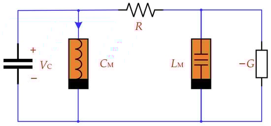
Figure 1.
Circuit schematic diagram of the hyperchaotic oscillator.
The equation for the state of the circuit can be expressed as [38]:
let x1 = vC, x2 = qM, x3 = φM, x4 = σ, x5 = ρ, the final dimensionless model of the circuit is obtained as
By introducing the Caputo differential definition, the fractional order form of the dimensionless equation for the above circuit can be written:
where q is the order of the FOMMS. Using the ADM algorithm, the linear and nonlinear terms of the FOMMS are decomposed as
According to Equation (7), the nonlinear terms of the system can be decomposed as
The initial condition is given as x0 = [x1(), x2(), x3(), x4(), x5()], and the first term can be written as
Letting = , = , = , = , = , it can be obtained that x0 = c0 = [ ]. By means of the iteration relation and the properties of the integral operator, it follows that
Let
Thus, x1 can be expressed as x1 = c1(t − t0)q/Γ(q + 1), and using the same method, the decomposition of the other term coefficients is shown in Appendix A.
Thus, the six-term numerical solution of FOMMS is
Setting the parameters q = 0.506, r = 0.2, g = 2, k = 1, a = 0.4, b = 2.8, d = 10, e = 3, the initial conditions are (1, 1, 0, 0, 0), and the iteration step h=0.001, it is obtained that the Lyapunov exponents of the system are LE1 = 7.3885, LE2 = 0.1046, LE3 = 0, LE4 = −6.0704 and LE5 = −171.3690, and the Lyapunov dimension is DL = 4.0622. The system has two positive Lyapunov exponents and can generate hyperchaotic attractors. The phase trajectories of hyperchaotic attractors of the system are illustrated in Figure 2. To demonstrate the diversity of attractors, the three-dimensional(3D) phase trajectories of chaotic attractors of this system and their projection to the two-dimensional(2D) plane are given in the figure.
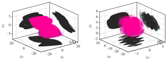
Figure 2.
3D phase diagram of the system and its projection in the 2D plane. (A) x1-x2-x3 phase space; (B) x3-x4-x5 phase space.
2.3. Dissipation and Stability of the System
The dissipation of the system can be solved by
Taking the given system parameters into Equation (22)
To obtain the equilibrium point of the system, let the left-hand side of the five-dimensional equation be equal to 0. The equation can be expressed as
Clearly, the system has a planar equilibrium point set E(0, 0, 0, m, n), and the Jacobian matrix of the system is deduced as
The characteristic equation for the equilibrium point is
where
A fractional order system is stable if the eigenvalues of the Jacobian matrix satisfy [39]
obviously E(0, 0, 0, 0, 0) is an equilibrium point of the system. Substituting the system parameters into the characteristic equations, the eigenvalues are obtained as λ1 = 0, λ2 = 0, λ3 = −5.3089 and λ4,5 = −0.5055 ± 1.7253i. At this time, the system is stable. When the equilibrium point is E(0, 0, 0, −π/2, −π/2), the eigenvalues of the system are obtained as λ1 = 0, λ2 = 0, λ3 = 2.104 and λ4,5 = −0.012 ± 5.8009i. The eigenvalue λ3 is a positive real number that falls on the real axis of the complex plane, so the equilibrium point is unstable.
3. Dynamical Analysis
3.1. Existence of Asymptotic Periodic Solutions for FO Systems
It has been shown that there are no exact periodic solutions for fractional order systems, but there are asymptotic periodic features in some fractional order systems.
Theorem 1
([40]). For fractional order differential equations
where i = 1, 2, …, n, 0 < q < 1. When the trajectory of the system in phase space satisfies limt→∞vi(t + T) − vi(t) = 0, T > 0, it is called an asymptotic periodic oscillation(A-P-O).
In this section, three typical parameters q, e and b of the FOMMS are chosen to investigate the effect of different orders and parameters on the dynamical behaviour of the system.
3.2. Bifurcation Diagrams (BD) and Lyapunov Exponent Spectrums (LEs) for Relevant Parameters
FO systems introduce integral operators and have more parameter choices compared to integer-order systems, and the maximum Lyapunov exponent becomes very large, i.e., chaotic enhancement occurs. This section examines the BD, LEs and fractional dimension of the three typical parameters, q, e and b, of the system in their adjustable intervals.
Case I: When the parameters r = 0.2, g = 2, k = 1, a = 0.4, b = 2.8, d = 10, e = 3, initial conditions are (1, 1, 0, 0, 0) and q varies in [0.5, 1], the system undergoes a tangent bifurcation evolution, including hyperchaos, asymptotic periodic oscillations and chaos, as shown in Figure 3. When q is in [0.5, 0.521], the system shows hyperchaotic behaviour and has the maximum Lyapunov value in the system, at which point it is a hyperchaotic state of type (I). When q is in [0.521, 0.553], the system enters (I)-type asymptotic periodic oscillations. When q is in [0.553, 1], the system exhibits chaotic phenomena, and the maximum Lyapunov exponent shows a decreasing trend as the value of q increases, exhibiting a chaotic phase space trajectory of type (I-IV) in turn. It should be noted that since the system LE5 is a very small negative value, it has been removed from the LEs in order to show the other four Lyapunov exponents of the system more clearly, as is the case in all the LEs below. The three types of dynamical behaviour in the system are summarised in Table 1, and the corresponding phase diagrams are depicted in Figure 4. As the value of q increases, the system completes the evolution from a hyperchaotic state to chaotic states. From the phase diagram, it can be found that the phase space trajectory of the hyperchaotic state is a superposition of the phase space trajectories of several chaotic states. It is clear from the LEs that the maximum Lyapunov exponent is much larger for FO systems than for integer-order systems.
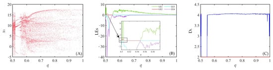
Figure 3.
Dynamical behaviour when the order q is varied. (A) BD; (B) LEs; (C) Lyapunov dimension.

Table 1.
Dynamical behaviour with respect to order q.
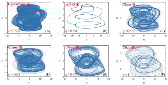
Figure 4.
The state of the attractor corresponding to a typical q value. (A) q = 0.506, Hyperchaos(I); (B) q = 0.531, A-P-O(I); (C) q = 0.572, Chaos(I); (D) q = 0.601, Chaos(II); (E) q = 0.677, Chaos(III); (F) q = 1, Chaos(IV).
Case II: When the parameters q = 0.7, r = 0.2, g = 2, k = 1, a = 0.4, b = 2.8, d = 10, initial conditions are (1, 1, 0, 0, 0), and the dynamical evolutionary behaviour of the system as e varies in [−5, 5] is given in Figure 5. Different system dynamical states are indicated in the bifurcation diagram by different zone colours, while arrows point out the bifurcation pattern when the bifurcation state of the system is changed. When e is in [−5, −4.14], the system exhibits asymptotic periodic oscillations of type (II). When e is in [−4.14, −3.84], the system exhibits (I)-type of asymptotic periodic oscillations. The jump switching between the two types of asymptotic periodic oscillations can be clearly seen in the BD. When e is in [−3.84, 0.7], the system transitions to a chaotic state via tangent bifurcation, exhibiting a (V)-type chaotic phase space trajectory during which there is a short asymptotic periodic window. When e is in [0.7, 1.04], the system exhibits (III)-type asymptotic periodic oscillations before transitions to a chaotic state via tangent bifurcation again. When e is in [1.04, 1.42], the system exhibits a (VI)-type chaotic phase space trajectory. When e is in [1.42, 5], the system exhibits a (III)-type chaotic phase space trajectory, and at e = 1.42, there is an interior crisis bifurcation that causes the chaotic state of the system to change in the range around this value. The resolution of typical states in the system is listed in Table 2, and the corresponding typical phase trajectory diagrams are shown in Figure 6. The (I)-type asymptotic periodic oscillations and (III)-type chaotic phase space trajectories are illustrated in Figure 3 and will not be shown repeatedly.
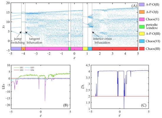
Figure 5.
Dynamical analysis in relation to parameter e. (A) BD; (B) LEs; (C) Lyapunov dimension.
Table 2.
Chaotic state with typical parameter e.
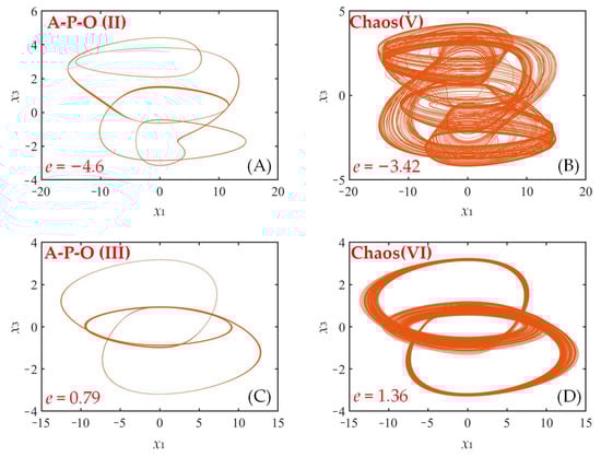
Figure 6.
Phase diagrams for different parameters e of FOMMS. (A) e = −4.6, A-P-O(II); (B) e = −3.42, Chaos(V); (C) e = 0.79, A-P-O(III); (D) e = 1.36, Chaos(VI).
Case III: The dynamical evolution of the system is shown in Figure 7; when the parameters are q = 0.7, r = 0.2, g = 2, k = 1, a = 0.4, d = 10, e = 3, the initial conditions are (1, 1, 0, 0, 0), and b varies in [2, 10]. When b is in [2, 2.252], the system exhibits (IV)-type asymptotic periodic oscillations. When b is in [2.252, 2.336], the system undergoes a very brief chaotic state, exhibiting (VII)-type chaotic phase space trajectories, and b enters (V)-type asymptotic periodic oscillations again when it is in [2.336, 2.476]. Then, the system transitions to a chaotic state through a tangent bifurcation, with the phase diagram evolving from (III) to (II) to (I)-type chaotic states when b is in [2.476, 3.696], and finally the system enters a hyperchaotic state when b is in [3.696, 10], exhibiting a (II)-type hyperchaotic phase space trajectory. A typical resolution of the system with respect to the parameter b is given by Table 3, while the corresponding phase diagram is plotted in Figure 8.
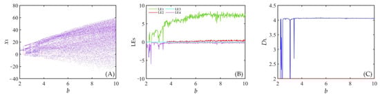
Figure 7.
Dynamical behaviour under changes in parameter b. (A) BD; (B) LEs; (C) Lyapunov dimension.
Table 3.
Dynamical behaviour of parameter b.
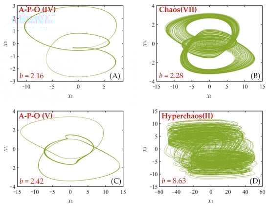
Figure 8.
Typical phase trajectory diagram for parameter b variation. (A) b = 2.16, A-P-O(IV); (B) b = 2.28, Chaos(VII); (C) b = 2.42, A-P-O(V); (D) b = 8.63, Hyperchaos(II).
3.3. Multiple Stability
3.3.1. Self-Reproduction of Attractors
The presence of the sine and cosine functions in the system makes the system inherently self-reproducing. The parameters are set to q = 0.7, r = 0.2, g = 2, k = 1, a = 0.4, b = 2.8, d = 10, e = 3. In this self-reproducing system, an infinite number of self-reproducing coexisting attractors can be generated, and only five sets of initial conditions are chosen symmetrically in the analysis. The state of the system controlled by the sine function manifested in x4 dimensions is shown in Figure 9. The initial conditions are x4(0) = kπ, k = (−8, −4, 0, 4, 8). The phase trajectory of the self-reproducing attractor in 3D space is shown in Figure 9A, while its projection in the 2D plane is plotted in Figure 9C, where the attractor can be seen to be periodically aligned along the x4 dimension. The corresponding BD for x4(0) in the (−8π, 8π) interval is shown in Figure 9B, where the dynamical evolution of the BD is linearly conditioned upwards in the intercepted interval. The corresponding time-domain waveforms are also depicted in Figure 9D, and the comparison shows that the mode of attractor reproduction and its time series signal are consistent with the performance of the BD. And the self-reproducing attractor controlled by the cosine function manifested in x5 dimensions is shown in Figure 10. The initial conditions are x5(0) = kπ, k = (−4, −2, 0, 2, 4). Similar to the x4 dimensional case, the combined analysis of Figure 10A–D, one by one, corresponds to the reproduction in the x5 dimensional system.
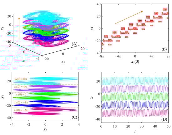
Figure 9.
Self-reproduction of attractors associated with the initial value x4. (A) 3D phase diagram; (B) BD for initial values; (C) 2D projection; (D) time-domain waveforms.
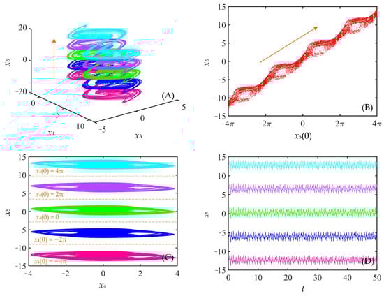
Figure 10.
Self-reproduction of attractors related to the initial value x5. (A) 3D phase diagram; (B) BD for initial values; (C) 2D projection; (D) time-domain waveforms.
3.3.2. Coexisting Attractors
Setting parameters q = 0.7, r = 0.2, g = 2, k = 1, a = 0.4, b = 2.8, d = 10, e = 3, and initial conditions of (1, x2(0), 0, 0, 0), the system has conditional coexistence behaviour, at which point the system exhibits coexistence behaviour of attractors different from the self-reproducing mode. The particular initial parameters chosen for the system in x2 dimensions cause the system to produce conditional homogeneous and heterogeneous multistability in phase space, with attractors advancing in either consistent or unequal steps. The coexistence of unequal-step heterogeneous attractors is shown in Figure 11A. Style (I) chaotic attractors alternate with style (II) chaotic attractors, and the attractors advance in the x2 direction in unequal steps. The coexistence of homogeneous style (I) chaotic attractors is shown in Figure 11B, where the system produces style (I) chaotic attractors and the attractors advance in the x2 direction in equal steps. The coexistence of homogeneous style (II) attractors is illustrated in Figure 11C, where this system produces style (II) chaotic attractors, and the attractors advance in the x2 dimension with unequal steps. The initial value of x2 at this point is indicated at the corresponding position of each attractor in the figure. Chaotic attractors with different initial conditions are shown in different colours, and the direction of advance of the chaotic attractor is indicated by the corresponding coloured arrow.
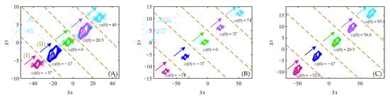
Figure 11.
The different types of coexisting attractors with respect to the initial condition x2 are shown in the x4-x5 phase. (A) Coexisting heterogeneous attractors with an unequal step; (B) Type (I) chaotic attractor coexistence; (C) Type (II) chaotic attractor coexistence.
3.4. State Transition
State transition is a special and complex phenomenon that occurs in chaotic systems. As time changes, the system state manifests itself as a transient or stable periodic or chaotic state, as a transition from one state to another. The process may be a transition from one periodic state to another periodic or chaotic (hyperchaotic) state or from one chaotic state to another periodic or chaotic (hyperchaotic) state. Given the initial conditions of (1, 1, 0, 0, 0), parameters q = 0.63, a = 0.32, b = 2.8, d = 10, e = 3, r = 0.2, g = 2, k = 1, the system state transition relationship is shown in Figure 12 and is composed of the time-domain waveform and x3-x4 phase diagram of the system. It is interesting to note that three chaotic state evolutions of the system occur during t at [0, 100]. When t is in [0, 42.263), this system is in chaotic state (I), indicated by light red. When t is in [42.263, 77.456), this system is in chaotic state (II), indicated by light blue. When t is in [77.456, 100], this system is in chaotic state (III), indicated in dark green. Therefore, the final chaotic attractor produced by the system is a light red double-scrolls chaotic attractor first, followed by a light blue double-scrolls chaotic attractor immediately based on it, which eventually manifests as a dark green four-scrolls chaotic attractor.
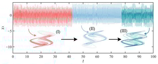
Figure 12.
State transition relations of the FOMMS.
4. Complexity Analysis
In the above analysis of a range of dynamical characteristics of the system, it can be seen that dynamical behaviour of the system is very complex. The complexity of FOMMS can be obtained using the SE algorithm. It provides convenience for the selection of system parameters in engineering applications. The darker the colour in the complexity diagram, the higher the complexity, indicating that the chaotic signal generated by the system in this parameter interval is closer to a random signal. Fixed parameters r = 0.2, g = 2, k = 1, a = 0.4, d = 10 with initial values of (1, 1, 0, 0, 0) were investigated for parameters (q, b, e) in the adjustable parameter interval with the two-parameter complexity diagram shown in Figure 13A–C. The initial complexity of the parameters r = 0.2, g = 2, k = 1, a = 0.4, d = 10, with initial conditions x4 in the interval [−8π, 8π] and x5 in the interval [−4π, 4π] was also examined as shown in Figure 13D. The 3D complexity gives an intuitive view of the variation in the high and low complexity of the system, while the 2D complexity diagram is better for the details of the different parameter intervals. Therefore, all things considered, the 3D complexity diagram of the system and its projection in the 2D phase space is given. It can be seen that the system has a relatively high complexity and a wide range of high complexity parameters.
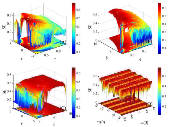
Figure 13.
Two-parameter complexity diagrams of the system in 3D, and its 2D projection. (A) q-e plane; (B) q-b plane; (C) b-e plane; (D) x4-x5 plane.
5. Hardware Implementation Based on DSP
The hardware implementation of chaotic systems is a prerequisite for their practical engineering application. In this section, the DSPF28335 is used as the core controller to implement the acquisition and transmission of FO chaotic systems. The DAC8552 is selected as the digital-to-analogue converter, and the corresponding phase trajectories are displayed via an oscilloscope. The equations of the FO chaotic system are written into the main function of the CCS integrated development environment. Setting parameters q = 0.7, r = 0.2, g = 2, k = 1, a = 0.4, b = 2.8, d = 10, e = 3 and initial conditions of (1, 1, 0, 0, 0), the processed chaotic signal is converted to analogue voltage through a digital-to-analogue converter and output to a two-channel oscilloscope. The hardware connection schematic of the experiment is shown in Figure 14, and the DSP hardware implementation platform is shown in Figure 15. The final experimental results obtained are shown in Figure 16 and Figure 17, which can prove that the simulation results are consistent with the results of the DSP hardware implementation.
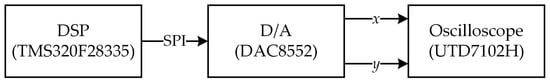
Figure 14.
The hardware connection schematic.
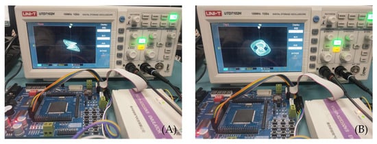
Figure 15.
DSP hardware implementation platform. (A) x1-x2 plane; (B) x3-x5 plane.
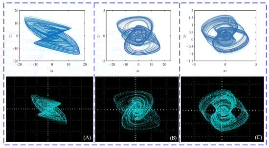
Figure 16.
Hardware implementation results. (A) x1-x2 plane; (B) x1-x3 plane; (C) x3-x5 plane.
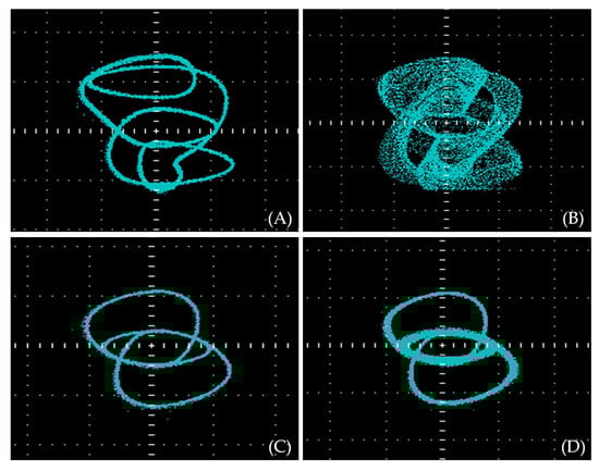
Figure 17.
Hardware implementation of typical phase trajectories under the variation of parameter e. (A) A-P-O(II); (B) Chaos(V); (C) A-P-O(III); (D) Chaos(VI).
6. Conclusions
The proposed memcapacitor meminductor hyperchaotic oscillator circuit is extended to a fractional order form and solved using the ADM algorithm. There are five types of A-P-O attractors, two types of hyperchaotic attractors and seven types of chaotic attractors that can be generated in the newly obtained FOMMS. The generation of hyperchaotic phenomena depends on the order of this system and the system parameters. Compared to the integer order system, the degrees of freedom of the system are extended and the maximum Lyapunov exponent is enhanced very significantly, verifying the chaos-enhancing behaviour of the fractional order system. Secondly, this system is multi-stable, and the system has the attractor coexistence behaviour in a self-reproducing manner. At the same time, there is a state transition phenomenon in the system; in a certain time interval, the system state has a chaotic state (I) to chaotic state (II) and finally to chaotic state (III), and chaotic state (I) and (II) exhibit double-scolls chaotic attractors, while chaotic state (III) exhibits four-scolls chaotic attractors, revealing the formation pattern of chaotic attractors. It is shown that FOMMS has a very complex dynamical behaviour. Finally, hardware implementation of the FOMMS based on DSP is carried out. The FOMMS proposed in this paper has good applications in the field of cryptography, and it is sincerely hoped that it can provide guidance for the study of high-dimensional FO chaotic systems. Next, it will be considered for application to the field of confidential communication.
Author Contributions
X.W.: Data curation, Formal analysis, Writing—original draft; B.L.: Conceptualisation, Project administration, Writing—review & editing; Y.C. and H.L.: Writing—review & editing. All authors have read and agreed to the published version of the manuscript.
Funding
This research received no external funding.
Data Availability Statement
Not applicable.
Acknowledgments
The authors thank the referees for their detailed reading and comments that were both helpful and insightful.
Conflicts of Interest
The authors declare no conflict of interest.
Appendix A
References
- Chua, L. Memristor-the missing circuit element. IEEE Trans. Circuit Theory 1971, 18, 507–519. [Google Scholar] [CrossRef]
- Di Ventra, M.; Pershin, Y.V.; Chua, L.O. Circuit elements with memory: Memristors, memcapacitors, and meminductors. Proc. IEEE 2009, 97, 1717–1724. [Google Scholar] [CrossRef]
- Ren, L.; Mou, J.; Banerjee, S.; Zhang, Y. A hyperchaotic map with a new discrete memristor model: Design, dynamical analysis, implementation and application. Chaos Solitons Fractals 2023, 167, 113024. [Google Scholar] [CrossRef]
- Xu, Q.; Lin, Y.; Bao, B.; Chen, M. Multiple attractors in a non-ideal active voltage-controlled memristor based Chua’s circuit. Chaos Solitons Fractals 2016, 83, 186–200. [Google Scholar] [CrossRef]
- Lin, H.; Wang, C.; Yu, F.; Sun, J.; Du, S.; Deng, Z.; Deng, Q. A review of chaotic systems based on memristive Hopfield neural networks. Mathematics 2023, 11, 1369. [Google Scholar] [CrossRef]
- Ma, Y.; Mou, J.; Lu, J.; Banerjee, S.; Cao, Y. A Discrete Memristor Coupled Two-Dimensional Generalized Square Hyperchaotic Maps. Fractals 2023, 31, 2340136. [Google Scholar] [CrossRef]
- Bao, H.; Chen, M.; Wu, H.; Bao, B. Memristor initial-boosted coexisting plane bifurcations and its extreme multi-stability reconstitution in two-memristor-based dynamical system. Sci. China Technol. Sci. 2020, 63, 603–613. [Google Scholar] [CrossRef]
- Ma, M.-L.; Xie, X.-H.; Yang, Y.; Li, Z.-J.; Sun, Y.-C. Synchronization coexistence in a Rulkov neural network based on locally active discrete memristor. Chin. Phys. B 2023, 32, 058701. [Google Scholar] [CrossRef]
- Guo, M.; Zhu, Y.; Liu, R.; Zhao, K.; Dou, G. An associative memory circuit based on physical memristors. Neurocomputing 2022, 472, 12–23. [Google Scholar] [CrossRef]
- Ma, T.; Mou, J.; Yan, H.; Cao, Y. A new class of Hopfield neural network with double memristive synapses and its DSP implementation. Eur. Phys. J. Plus 2022, 137, 1135. [Google Scholar] [CrossRef]
- Gao, X.; Sun, B.; Cao, Y.; Banerjee, S.; Mou, J. A color image encryption algorithm based on hyperchaotic map and DNA mutation. Chin. Phys. B 2023, 32, 030501. [Google Scholar] [CrossRef]
- de la Fraga, L.G.; Ovilla-Martínez, B. A chaotic PRNG tested with the heuristic Differential Evolution. Integration 2023, 90, 22–26. [Google Scholar] [CrossRef]
- Echenausía-Monroy, J.L.; Campos, E.; Jaimes-Reátegui, R.; García-López, J.H.; Huerta-Cuellar, G. Deterministic Brownian-like motion: Electronic approach. Electronics 2022, 11, 2949. [Google Scholar] [CrossRef]
- De la Fraga, L.G. Analyzing All the Instances of a Chaotic Map to Generate Random Numbers. Comput. Sci. Math. Forum 2022, 4, 6. [Google Scholar]
- Wang, L.; Cao, Y.; Jahanshahi, H.; Wang, Z.; Mou, J. Color image encryption algorithm based on Double layer Josephus scramble and laser chaotic system. Optik 2023, 275, 170590. [Google Scholar] [CrossRef]
- Ma, X.; Wang, C.; Qiu, W.; Yu, F. A fast hyperchaotic image encryption scheme. Int. J. Bifurc. Chaos 2023, 33, 2350061. [Google Scholar] [CrossRef]
- Sha, Y.; Mou, J.; Banerjee, S.; Zhang, Y. Exploiting Flexible and Secure Cryptographic Technique for Multi-Dimensional Image Based on Graph Data Structure and Three-Input Majority Gate. IEEE Trans. Ind. Inform. 2023. [Google Scholar] [CrossRef]
- Zhu, Y.; Wang, C.; Sun, J.; Yu, F. A chaotic image encryption method based on the artificial fish swarms algorithm and the DNA coding. Mathematics 2023, 11, 767. [Google Scholar] [CrossRef]
- Ma, X.; Wang, C. Hyper-chaotic image encryption system based on N+ 2 ring Joseph algorithm and reversible cellular automata. Multimed. Tools Appl. 2023. [Google Scholar] [CrossRef]
- Gao, X.; Mou, J.; Banerjee, S.; Zhang, Y. Color-Gray Multi-Image Hybrid Compression–Encryption Scheme Based on BP Neural Network and Knight Tour. IEEE Trans. Cybern. 2023, 53, 5037–5047. [Google Scholar] [CrossRef]
- Sha, Y.; Mou, J.; Wang, J.; Banerjee, S.; Sun, B. Chaotic image encryption with Hopfield neural network. Fractals 2023, 31, 2340107. [Google Scholar] [CrossRef]
- Sheng, Z.; Li, C.; Gao, Y.; Li, Z.; Chai, L. A Switchable Chaotic Oscillator with Multiscale Amplitude/Frequency Control. Mathematics 2023, 11, 618. [Google Scholar] [CrossRef]
- Ghanbari, B.; Günerhan, H.; Srivastava, H. An application of the Atangana-Baleanu fractional derivative in mathematical biology: A three-species predator-prey model. Chaos Solitons Fractals 2020, 138, 109910. [Google Scholar] [CrossRef]
- Han, X.; Mou, J.; Lu, J.; Banerjee, S.; Cao, Y. Two discrete memristive chaotic maps and its DSP implementation. Fractals 2023, 31, 2340104. [Google Scholar] [CrossRef]
- Xu, S.; Wang, X.; Ye, X. A new fractional-order chaos system of Hopfield neural network and its application in image encryption. Chaos Solitons Fractals 2022, 157, 111889. [Google Scholar] [CrossRef]
- Huang, P.; Chen, X.; Chai, Y.; Ma, L. A unified framework of fault detection and diagnosis based on fractional-order chaos system. Aerosp. Sci. Technol. 2022, 130, 107871. [Google Scholar] [CrossRef]
- Akgul, A.; Rajagopal, K.; Durdu, A.; Pala, M.A.; Yldz, M.Z. A simple fractional-order chaotic system based on memristor and memcapacitor and its synchronization application. Chaos Solitons Fractals 2021, 152, 111306. [Google Scholar] [CrossRef]
- Ma, T.; Mou, J.; Li, B.; Banerjee, S.; Yan, H. Study on the complex dynamical behavior of the fractional-order hopfield neural network system and its implementation. Fractal Fract. 2022, 6, 637. [Google Scholar] [CrossRef]
- Zhou, N.-R.; Tong, L.-J.; Zou, W.-P. Multi-image encryption scheme with quaternion discrete fractional Tchebyshev moment transform and cross-coupling operation. Signal Process. 2023, 211, 109107. [Google Scholar] [CrossRef]
- Liu, X.; Mou, J.; Wang, J.; Banerjee, S.; Li, P. Dynamical analysis of a novel fractional-order chaotic system based on memcapacitor and meminductor. Fractal Fract. 2022, 6, 671. [Google Scholar] [CrossRef]
- Echenausía-Monroy, J.; Jafari, S.; Huerta-Cuellar, G.; Gilardi-Velázquez, H. Predicting the emergence of multistability in a Monoparametric PWL system. Int. J. Bifurc. Chaos 2022, 32, 2250206. [Google Scholar] [CrossRef]
- Liu, X.; Mou, J.; Zhang, Y.; Cao, Y. A New Hyperchaotic Map Based on Discrete Memristor and Meminductor: Dynamics Analysis, Encryption Application, and DSP Implementation. IEEE Trans. Ind. Electron. 2023. [Google Scholar] [CrossRef]
- Li, Y.; Li, C.; Zhang, S.; Chen, G.; Zeng, Z. A self-reproduction hyperchaotic map with compound lattice dynamics. IEEE Trans. Ind. Electron. 2022, 69, 10564–10572. [Google Scholar] [CrossRef]
- Gao, X.; Mou, J.; Li, B.; Banerjee, S.; Sun, B. Multi-image hybrid encryption algorithm based on pixel substitution and gene theory. Fractals 2023, 31, 2340111. [Google Scholar] [CrossRef]
- Bao, H.; Hua, Z.; Wang, N.; Zhu, L.; Chen, M.; Bao, B. Initials-boosted coexisting chaos in a 2-D sine map and its hardware implementation. IEEE Trans. Ind. Inform. 2020, 17, 1132–1140. [Google Scholar] [CrossRef]
- Kilbas, A.A.; Marzan, S.A. Nonlinear differential equations with the Caputo fractional derivative in the space of continuously differentiable functions. Differ. Equ. 2005, 41, 84–89. [Google Scholar] [CrossRef]
- Cherruault, Y.; Adomian, G. Decomposition methods: A new proof of convergence. Math. Comput. Model. 1993, 18, 103–106. [Google Scholar] [CrossRef]
- Wang, X.; Mou, J.; Jahanshahi, H.; Alotaibi, N.D.; Bi, X. Extreme multistability arising from periodic repetitive bifurcation behavior in a hyperchaotic oscillator. Nonlinear Dyn. 2023, 111, 13561–13578. [Google Scholar] [CrossRef]
- Matignon, D. Stability results for fractional differential equations with applications to control processing. In Proceedings of the Computational Engineering in Systems Applications, Lille, France, 9–12 July 1996; pp. 963–968. [Google Scholar]
- Danca, M.-F.; Fečkan, M.; Kuznetsov, N.V.; Chen, G. Complex dynamics, hidden attractors and continuous approximation of a fractional-order hyperchaotic PWC system. Nonlinear Dyn. 2018, 91, 2523–2540. [Google Scholar] [CrossRef]


Disclaimer/Publisher’s Note: The statements, opinions and data contained in all publications are solely those of the individual author(s) and contributor(s) and not of MDPI and/or the editor(s). MDPI and/or the editor(s) disclaim responsibility for any injury to people or property resulting from any ideas, methods, instructions or products referred to in the content. |
© 2023 by the authors. Licensee MDPI, Basel, Switzerland. This article is an open access article distributed under the terms and conditions of the Creative Commons Attribution (CC BY) license (https://creativecommons.org/licenses/by/4.0/).