Evolution Analysis of Strain Waves for the Fractal Nonlinear Propagation Equation of Longitudinal Waves in a Rod

Abstract

Based on the layered and porous characteristics of functionally graded materials and the finite deformation assumption of solids, the fractal nonlinear propagation equation of longitudinal waves in a functionally graded rod is derived. A large number of exact displacement gradient traveling wave solutions of the fractal equation are obtained by using an equivalent simplified extended (G′/G) expansion method. Three sets of existing and different displacement gradient solutions are obtained by analyzing these exact solutions, and then three corresponding fractal dimension strain waves are derived. The results of numerical simulation of the evolution of these three strain waves with fractal dimension show that when the strain wave propagates in the rod, the smaller the fractal dimension or, the larger the radius of the rod, the higher the tensile strength of the material.

1. Introduction

Due to the good performance and designability of functionally graded materials, it is widely used in engineering structures in the aerospace industry, defense industry, electronics industry, chemical engineering, biomedical engineering, and other fields [1,2]. When the wave propagates in functionally graded materials, it is bound to carry information about its internal structural properties, which will be reflected by waveform, amplitude, and wave velocity. The study of wave propagation in functionally graded materials has attracted the attention of scholars at home and abroad. For example, Gupta [3] conducted research on the propagation behavior of Love waves in layered structures of functionally graded materials, Kielczynski [4] discussed the propagation behavior of ultrasonic Love waves in inhomogeneous functionally graded elastic materials, and Chen [5] studied the propagation characteristics of linear waves in functionally graded materials with layered structure by using the layered theory. In fact, due to the lack of preparation methods and processes, the prepared functionally graded materials often have many tiny pores [6,7]. Some scholars have studied the static and dynamic response of porous functionally graded materials based on porous volume fraction, functional gradient index, and porosity distribution patterns [8,9,10,11]. According to fractal geometry, a layered structure or porous media can be seen as a fractal medium [12]. The fractal derivative proposed by He [13,14] based on the analysis of the distance change between two points in fractal media is a new powerful modeling tool, which has been applied to the establishment of differential models in hierarchical structures or porous media and the analysis of some phenomena [15,16,17,18,19].

The constant cross-section elastic rod is the most important structural element in the application. The linear wave theory is an approximation under many assumptions. For high-speed or heavy-load impact, it is found that the finite deformation assumption will be more reasonable [20]. Many new phenomena can only be understood at the nonlinear level [21,22]. In nonlinear wave problems, it is very important to find the exact solutions of nonlinear wave equations because the exact solutions of nonlinear wave equations can not only graphically display many complex nonlinear phenomena but also allow the interpretation of their mechanism. It is also an important basis for the study of other problems [23]. In engineering wave problems, the exact solution of the high-dimensional model of wave propagation has more significant applications [24,25,26,27]. For the solution of nonlinear equations, after the efforts of relevant scholars in recent decades, many accurate methods have been developed, such as inverse scattering method [28], hyperbolic tangent method [29], extended hyperbolic function method [30,31,32], Jacobi elliptic function expansion method and its extended form [33,34,35], F-function expansion method [36], exponential function method [37], Kudryashov method [38], Riccati function expansion method [39], Khater method [40], sine-cosine method [41], (G′/G) function expansion method [42,43], (G′/G,1/G) function expansion method [44], (1/G) function expansion method [45], (1/G’) function expansion method [46], (G′/G2) function expansion method [47], extended (G′/G) function expansion method [48,49]. Among these methods, the extended (G′/G) expansion method [48] is relatively simple, but the author of this method has not carefully studied the mechanism of the extended (G′/G) expansion method to obtain new forms of exact solutions compared with the (G′/G) expansion method.

Due to the complexity of mathematics, the research results of nonlinear wave propagation in functionally graded materials are rare, and there are fewer analytical studies. However, the study of nonlinear wave propagation will reveal many interesting and important phenomena [50,51,52]. And because media with layered structure and porous characteristics can be approximated as fractal media [12,15,16,17,18,19], the research work in this article has been carried out. Different from previous studies, this paper studies the propagation of nonlinear longitudinal waves in functional gradient bars with layered structure and porous characteristics based on fractal, which mainly involves the derivation of the fractal nonlinear propagation model equation of longitudinal waves and the acquisition of the exact solution of the equation, the acquisition of existing and independent fractal dimension strain waves, and the numerical simulation analysis of fractal dimension strain waves. This will help to further study the dynamic behavior and performance of mechanical components with rod-shaped structures based on wave propagation. The main contributions are as follows.

• Based on the layered and porous characteristics of functionally graded materials, a fractal nonlinear propagation equation for longitudinal waves in a functionally graded rod is established for the first time using fractal derivatives. Due to the joint intervention of nonlinearity and fractal, the derivation of the longitudinal wave propagation equation in the rod is more technical.
• An equivalent simplified extension (G′/G) expansion method is proposed and used to obtain the exact displacement gradient traveling wave solution of the fractal nonlinear propagation equation of longitudinal waves in the functional gradient rod. This equivalent simplification makes the solution process more concise.
• By comparing and discussing all the exact solutions obtained and analyzing the mechanism of the solution method, it is clarified which forms of exact solutions of the nonlinear wave equation can be obtained by the extended (G′/G) expansion method. This makes the understanding of the extended (G’ G) expansion method more profound.
• Through numerical simulation, the evolution law of three kinds of fractal dimension strain waves in functionally graded rods with space-time fractal dimension is shown, and the performance requirements of the materials when the strain waves propagate in functionally graded materials are found. This makes the presentation of the conclusion more intuitive.

The rest of this paper is arranged as follows: In Section 2, the fractal nonlinear longitudinal wave propagation equation in the rod is derived. In Section 3, the exact displacement gradient traveling wave solution of the fractal nonlinear longitudinal wave propagation equation in the rod is obtained by using the equivalent simplified extended (G′/G) expansion method. In Section 4, the 26 exact solutions obtained by the extended (G′/G) method are compared and discussed, and the results obtained from the discussion are theoretically analyzed from the perspective of the solution method. In Section 5, the evolution of nonlinear strain wave with space-time fractal dimension is discussed by numerical simulation. Finally, in Section 6, the conclusion of this paper is given.

2. Fractal Nonlinear Propagation Equation of Longitudinal Waves in a Rod

In this section, considering the finite deformation, Poisson effect, layered and porous characteristics of functionally graded materials and fractal derivatives, the Lagrange material description and cylindrical coordinate system $(x,r,\theta )$ are used to derive the fractal nonlinear propagation equation of longitudinal waves in a functionally graded circular cross-section thin rod in fractal space-time, where x is the axial coordinate, and r and θ are radial and circumferential coordinates, respectively. The fractal derivative used is defined as follows [14].

$$\frac{df}{d{x}^{\alpha }}=\underset{\Delta x=x_A-x_B\to L_0}{\lim }\frac{f(A)-f(B)}{x_A^{\alpha }-x_B^{\alpha }},$$

(1)

the definition of Formula (1) regards the fractal medium as a fractal space. The distance between A and B in the fractal space will no longer be the straight line distance $x_A-x_B$ in the continuous medium space, but $x_A^{\alpha }-x_B^{\alpha }$ (see Equation (47) of [12]).

It is assumed that the time fractal dimension index is $\alpha$, the space fractal dimension index is $\beta$, the radius of the fractal thin rod (functional gradient circular cross-section thin rod) is R, and the material density is ρ. Based on the fractal invariance and fractal equivalence assumptions [53,54], the fractal thin rod is in an axisymmetric compression state during the longitudinal motion (displacement, strain, and stress are independent of θ), and the Navier-Bernolli and Love assumptions are still used. Therefore, the axial displacement $D=D(x,t)={}_{x}D(x,t)$ is independent of r, and the radial displacement can be taken as ${}_{r}D=-\nu r^{\beta }{D}_x^{\beta }$, where $D_x^{\beta }=\partial D/\partial x^{\beta }$, $\nu$ is the Poisson ratio, and t is the time coordinate. Considering that the radial displacement is a higher order quantity of the axial displacement, the transverse shear strain expressed by the displacement is $\gamma ={}_{r}D{}_x^{\beta }=-\nu r^{\beta }{D}_{xx}^{\beta \beta }$.

The motion of the fractal thin rod is axisymmetric compression. Because the transverse effect is considered, the kinetic energy per unit length of the fractal elastic rod is the sum of the longitudinal kinetic energy and the transverse kinetic energy.

$$\begin{array}{ll}\hfill T& ={\displaystyle {\int }_0^R{(D_t{}^{\alpha })}^2\frac{1}{2}}\rho 2\pi r^{\beta }d{r}^{\beta }+{\displaystyle {\int }_0^R{(-\nu r{D}_{tx}{}^{\alpha \beta })}^2\frac{1}{2}}\rho 2\pi r^{\beta }d{r}^{\beta }\\ & =\frac{1}{2}\rho A^{\beta }{(D_t{}^{\alpha })}^2+\frac{1}{4}\rho A^{\beta }{R}^2{\nu }^2{(D_{tx}{}^{\alpha \beta })}^2,\end{array}$$

(2)

where $A^{\beta }=\pi R^{2\beta }$ is the cross-sectional area of the fractal thin rod.

In the one-dimensional case, considering the influence of finite deformation, the axial strain-displacement relationship is as follows.

$${\epsilon }_x=D_x{}^{\beta }+0.5{(D_x{}^{\beta })}^2$$

(3)

The stress-strain relationship is based on Hooke’s law. Due to the transverse effect, the strain energy per unit length of the finite deformation fractal elastic rod is composed of longitudinal compressive strain energy and transverse shear strain energy.

$$\begin{array}{ll}\hfill W& ={\displaystyle {\int }_0^{{\epsilon }_x}{\displaystyle {\int }_0^R\sigma ({\epsilon }_x)}2\pi r^{\beta }d{r}^{\beta }}d{\epsilon }_x+{\displaystyle {\int }_0^R{\displaystyle {\int }_0^{\gamma }G\gamma }}d\gamma 2\pi r^{\beta }d{r}^{\beta }\\ & =\frac{1}{2}{A}^{\beta }E{\left(D_x{}^{\beta }+\frac{1}{2}{(D_x{}^{\beta })}^2\right)}^2+\frac{1}{4}G{\nu }^2{A}^{\beta }{R}^{2\beta }{\left(D_{xx}{}^{\beta \beta }\right)}^2,\end{array}$$

(4)

where $\sigma$ is the axial stress, E is the elastic modulus, and G is the shear modulus.

According to Hamilton’s variational principle, there are

$$\delta {\displaystyle {\int }_{t_1}^{t_2}{\displaystyle {\int }_{x_1}^{x_2}L}d{x}^{\beta }d{t}^{\alpha }}=\delta {\displaystyle {\int }_{t_1}^{t_2}{\displaystyle {\int }_{x_1}^{x_2}(T-V)}d{x}^{\beta }d{t}^{\alpha }}=0,$$

(5)

where $L=T-W$ is the Lagrange density function. Bringing Equations (2) and (4) into Equation (5) and then variational operation item by item, the longitudinal wave equation of the finite deformation fractal elastic thin rod is obtained as follows.

$$\rho D_{tt}{}^{\alpha \alpha }-\frac{1}{2}\rho R^{2\beta }{\nu }^2{D}_{xttx}{}^{\beta \alpha \alpha \beta }-\frac{1}{2}E{\left(2D_x{}^{\beta }+3{(D_x{}^{\beta })}^2+{(D_x{}^{\beta })}^3\right)}_x{}^{\beta }+\frac{1}{2}G{\nu }^2{R}^{2\beta }{D}_{xxxx}{}^{\beta \beta \beta \beta }=0.$$

(6)

Equation (6) is a wave equation with double nonlinear and double dispersion. It contains not only two geometric dispersion effects of transverse inertia and transverse shear but also two nonlinear terms. The second term is the dispersion term caused by transverse inertia caused by the Poisson effect. The two nonlinear terms in the third term are caused by longitudinal geometric nonlinearity. The fourth term is the dispersion term caused by transverse shear caused by the Poisson effect. Under the condition of model derivation, we can try to apply our model in the field of mechanical dynamics, such as studying the dynamic behavior of mechanical components with rod structure. Take the displacement gradient $D_x{}^{\beta }=u$, and then sort out Equation (6) to obtain

$$u_{tt}{}^{\alpha \alpha }-\frac{E}{\rho }{u}_{xx}{}^{\beta \beta }-{\left(\frac{3E}{2\rho }{u}^2+\frac{E}{2\rho }{u}^3+\frac{1}{2}{R}^{2\beta }{\nu }^2(u_{tt}{}^{\alpha \alpha }-\frac{G}{\rho }{u}_{xx}{}^{\beta \beta })\right)}_{xx}{}^{\beta \beta }=0,$$

(7)

Here, we equate the influence of the ‘anomaly’ of the functionally graded rod compared with the ordinary rod on the mechanical properties of the rod with the influence of the fractal space-time transformation, thus establishing the fractal nonlinear longitudinal wave propagation equation. When the wave propagates in the functionally graded rod, it is bound to carry information about its internal structural properties, which will be reflected by the waveform, amplitude, and wave velocity. In the traveling wave solution of Equation (7), there must be space-time fractal dimension indexes $\alpha$ and $\beta$, which means that we can study the evolution of the longitudinal wave through the fractal dimension index. Furthermore, the dynamic performance of functionally graded rod-shaped mechanical components can be studied by studying this longitudinal wave.

3. Exact Displacement Gradient Traveling Wave Solutions of the Fractal Nonlinear Longitudinal Wave Propagation Equation

In this section, we will use the extended (G′/G) expansion method to obtain the exact traveling wave solution of Equation (7). In the solution process, the more concise equivalent auxiliary equation $G^{″}+hG=0$ is used. Through the general solution of the auxiliary equation, the solutions of (G′/G) under different conditions are obtained as follows.

$$\left(\frac{G^{\prime }}{G}\right)=\{\begin{array}{l}\sqrt{-h}\left(C_1\sinh \left(\sqrt{-h}\xi \right)+C_2\cosh \left(\sqrt{-h}\xi \right)\right)/\left(C_1\cosh \left(\sqrt{-h}\xi \right)+C_2\sinh \left(\sqrt{-h}\xi \right)\right),h<0\\ \sqrt{h}\left(-C_1\sin \left(\sqrt{h}\xi \right)+C_2\cos \left(\sqrt{h}\xi \right)\right)/\left(C_1\cos \left(\sqrt{h}\xi \right)+C_2\sin \left(\sqrt{h}\xi \right)\right),h>0\\ C_2/(C_1+C_2\xi ),h=0\end{array},$$

(8)

where C₁ and C₂ are free constants, the results of (8) can be rewritten as follows.

$$\left(\frac{G^{\prime }}{G}\right)=\{\begin{array}{l}\sqrt{-h}\tanh \left(\sqrt{-h}\xi +{\xi }_0\right),h<0,\tanh ({\xi }_0)=C_2/C_1,\left|C_2/C_1\right|<1\\ \sqrt{-h}\coth \left(\sqrt{-h}\xi +{\xi }_0\right),h<0,\coth ({\xi }_0)=C_2/C_1,\left|C_2/C_1\right|>1\\ \sqrt{h}\cot \left(\sqrt{h}\xi +{\xi }_0\right),h>0,\cot ({\xi }_0)=C_2/C_1\\ -\sqrt{h}\tan \left(\sqrt{h}\xi +{\xi }_0\right),h>0,\tan ({\xi }_0)=-C_2/C_1\\ C_2/(C_1+C_2\xi ),h=0\end{array}.$$

(9)

The fractal traveling wave transformation $u(x,t)=U(\xi ),\xi =x^{\beta }-{(ct)}^{\alpha }$ is made for Equation (7), and then

$$R^{2\beta }{\nu }^2(c^{2\alpha }-\frac{G}{\rho })U^{⁗}-2(c^{2\alpha }-\frac{E}{\rho })U^{″}+\frac{3E}{\rho }2({(U^{\prime })}^2+U{U}^{″})+\frac{E}{\rho }3(U^2{U}^{″}+2U{(U^{\prime })}^2)=0.$$

(10)

Taking

$$p_1=\left(-2(c^{2\alpha }-E/\rho )\right)/\left(R^{2\beta }{\nu }^2(c^{2\alpha }-G/\rho )\right),p_2=3E/\rho R^{2\beta }{\nu }^2(c^{2\alpha }-G/\rho ),$$

(11)

then the Equation (10) becomes

$$U^{⁗}+p_1{U}^{″}+2p_2({(U^{\prime })}^2+U{U}^{″})+p_2(U^2{U}^{″}+2U{(U^{\prime })}^2)=0.$$

(12)

According to the homogeneous balance principle, the highest order derivative term $U^{″″}$ and the nonlinear term $U^2{U}^{″}$ are balanced, and the proposed solution of the extended (G′/G) expansion method can be obtained as

$$U(\xi )=a_0+a_1\frac{G^{\text{'}}}{G}+b_1{\left(\frac{G^{\text{'}}}{G}\right)}^{-1}.$$

(13)

Bring Equation (13) into Equation (12), collect the coefficients of all power terms of the (G′/G) function, and let them be zero. The following nonlinear algebraic equations are obtained.

$${\left(G^{\prime }/G\right)}^{-5}:4h^2{b}_1^3{p}_2+24h^4{b}_1=0, {\left(G^{\prime }/G\right)}^{-4}:6h^2{a}_0{b}_1^2{p}_2+6h^2{b}_1^2{p}_2=0,$$

$${\left(G^{\prime }/G\right)}^{-3}:2h^2{a}_0^2{b}_1{p}_2+2h^2{a}_1{b}_1^2{p}_2+4h^2{a}_0{b}_1{p}_2+6h{b}_1^3{p}_2+40h^3{b}_1+2h^2{b}_1{p}_1=0,$$

$${\left(G^{\prime }/G\right)}^{-2}:8h{a}_0{b}_1^2{p}_2+8h{b}_1^2{p}_2=0,$$

$${\left(G^{\prime }/G\right)}^{-1}:2h{a}_0^2{b}_1{p}_2+2h{a}_1{b}_1^2{p}_2+4h{a}_0{b}_1{p}_2+2b_1^3{p}_2+16h^2{b}_1+2h{b}_1{p}_1=0,$$

$${\left(G^{\prime }/G\right)}^0:2h^2{a}_0{a}_1^2{p}_2+2h^2{a}_1^2{p}_2+2a_0{b}_1^2{p}_2+2b_1^2{p}_2=0,$$

$${\left(G^{\prime }/G\right)}^1:2h^2{a}_1^3{p}_2+2h{a}_0^2{a}_1{p}_2+2h{a}_1^2{b}_1{p}_2+4h{a}_0{a}_1{p}_2+16h^2{a}_1+2h{a}_1{p}_1=0,$$

$${\left(G^{\prime }/G\right)}^2:8h{a}_0{a}_1^2{p}_2+8h{a}_1^2{p}_2=0,$$

$${\left(G^{\prime }/G\right)}^3:6h{a}_1^3{p}_2+2a_0^2{a}_1{p}_2+2a_1^2{b}_1{p}_2+4a_0{a}_1{p}_2+40h{a}_1+2a_1{p}_1=0,$$

$${\left(G^{\prime }/G\right)}^4:6a_0{a}_1^2{p}_2+6a_1^2{p}_2=0,$$

$${\left(G^{\prime }/G\right)}^5:4a_1^3{p}_2+24a_1=0.$$

The following four groups of nontrivial solutions are obtained by solving the nonlinear algebraic equations composed of the above 11 equations.

$$a_0=-1,a_1=\pm \sqrt{-6/p_2},b_1=\pm \sqrt{-6h^2/p_2},2h-6\left|h\right|=p_2-p_1.$$

(14)

$$a_0=-1,a_1=\pm \sqrt{-6/p_2},b_1=\mp \sqrt{-6h^2/p_2},2h+6\left|h\right|=p_2-p_1.$$

(15)

$$a_0=-1,a_1=\pm \sqrt{-6/p_2},b_1=0,2h=p_2-p_1.$$

(16)

$$a_0=-1,a_1=0,b_1=\pm \sqrt{-6h^2/p_2},2h=p_2-p_1.$$

(17)

By substituting the values of Equations (14)–(17) into Equation (13) respectively and combining Equation (8) or Equation (9), different exact solutions of Equation (12) under different parameter conditions are obtained. Combined with the fractal traveling wave transformation, the exact traveling wave solutions of Equation (7) can be obtained.

For the coupled solution set of Equation (14):

(1)

When h < 0, using Equation (8) or Equation (9), the exact hyperbolic function solutions of Equation (7) are obtained as follows.

$$u_{1,2}(x,t)=-1\pm 2\sqrt{6h/p_2}\coth \left(2(\sqrt{-h}(x^{\beta }-{(ct)}^{\alpha })+{\xi }_0)\right).$$

(2)

When h > 0, using Equation (8) or Equation (9), the exact solution of the trigonometric function of Equation (7) is obtained as follows.

$$u_{3,4}(x,t)=-1\pm 2\sqrt{-6h/p_2}\csc \left[2\left(\sqrt{h}(x^{\beta }-{(ct)}^{\alpha })+{\xi }_0\right)\right].$$

(18)

(3)

When h = 0, then b₁ = 0, the rational solution of Equation (7) is

$$u_{5,6}(x,t)=-1\pm \sqrt{-6/p_2}{C}_2/\left(C_1+C_2(x^{\beta }-{(ct)}^{\alpha })\right).$$

For the coupled solution set of Equation (15):

(1)

When h < 0, using Equation (8) or Equation (9), the exact hyperbolic function solutions of Equation (7) are obtained as follows.

$$u_{7,8}(x,t)=-1\pm 2\sqrt{6h/p_2}\csc \mathrm{h}\left[2\left(\sqrt{-h}(x^{\beta }-{(ct)}^{\alpha })+{\xi }_0\right)\right].$$

(2)

When h > 0, using Equation (8) or Equation (9), the exact solution of the trigonometric function of Equation (7) is obtained as follows.

$$u_{9,10}(x,t)=-1\pm 2\sqrt{-6h/p_2}\tan \left(2\sqrt{h}(x^{\beta }-{(ct)}^{\alpha })+2{\xi }_0\right).$$

(3)

When h = 0, then $b_1=0$, the solution is the previous solution $u_{5,6}(x,t)$.

For the solution group of Equation (16):

(1)

When h < 0, using Equation (8) or Equation (9), the exact hyperbolic function solutions of Equation (7) are obtained as follows.

$$u_{11,12}(x,t)=-1\pm 2\sqrt{6h/p_2}\coth \left(2\sqrt{-h}(x^{\beta }-{(ct)}^{\alpha })+{\xi }_0\right),\left|C_2/C_1\right|>1,$$

$$u_{13,14}(x,t)=-1\pm 2\sqrt{6h/p_2}\tanh \left(2\sqrt{-h}(x^{\beta }-{(ct)}^{\alpha })+{\xi }_0\right),\left|C_2/C_1\right|<1.$$

(19)

(2)

When h > 0, using Equation (8) or Equation (9), the exact solution of the trigonometric function of Equation (7) is obtained as follows.

$$u_{15,16}(x,t)=-1\pm 2\sqrt{-6h/p_2}\cot \left(2\sqrt{h}(x^{\beta }-{(ct)}^{\alpha })+{\xi }_0\right),{\xi }_0=arc\cot (C_2/C_1),$$

$$u_{17,18}(x,t)-1\pm 2\sqrt{-6h/p_2}\tan \left(2\sqrt{h}(x^{\beta }-{(ct)}^{\alpha })+{\xi }_0\right),{\xi }_0=-\arctan (C_2/C_1).$$

(3)

When h = 0, the solution is the previous solution $u_{5,6}(x,t)$.

For the solution group of Equation (17):

(1)

When h < 0, using Equation (8) or Equation (9), the exact hyperbolic function solutions of Equation (7) are obtained as follows.

$$u_{19,20}(x,t)=-1\pm 2\sqrt{6h/p_2}\tanh \left(2\sqrt{-h}(x^{\beta }-{(ct)}^{\alpha })+{\xi }_0\right),\left|C_2/C_1\right|>1,$$

$$u_{21,22}(x,t)=-1\pm 2\sqrt{6h/p_2}\coth \left(2\sqrt{-h}(x^{\beta }-{(ct)}^{\alpha })+{\xi }_0\right),\left|C_2/C_1\right|<1.$$

(20)

(2)

When h > 0, using Equation (8) or Equation (9), the exact solution of the trigonometric function of Equation (7) is obtained as follows.

$$u_{23,24}(x,t)=-1\pm 2\sqrt{-6h/p_2}\tan \left(2\sqrt{h}(x^{\beta }-{(ct)}^{\alpha })+{\xi }_0\right),{\xi }_0=arc\cot (C_2/C_1),$$

$$u_{25,26}(x,t)=-1\pm 2\sqrt{-6h/p_2}\cot \left(2\sqrt{h}(x^{\beta }-{(ct)}^{\alpha })+{\xi }_0\right),{\xi }_0=-\arctan (C_2/C_1).$$

(3)

When h = 0, then b₁ = 0, the solution degenerates into a constant.

4. Discussion of Exact Solution and Solving Method

In this section, we first compare and discuss the 26 accurate displacement gradient solutions obtained by the extended (G′/G) method in the previous section and draw some phenomena conclusions. Secondly, these conclusions are theoretically analyzed from the perspective of the solution method.

4.1. Comparative Discussion of Exact Displacement Gradient Solutions

It can be seen that Equation (16) is the solution group obtained by the (G′/G) expansion method, and Equation (17) is the solution group obtained by the (G/G′) open method.

The parameters C₁ and C₂ are arbitrary, and the phase ${\xi }_0$ causes the translation of the traveling wave. Therefore, when considering whether the two traveling waves are equivalent, the phase ${\xi }_0$ is ignored. It follows that, firstly, the solutions u_11,12 and u_17,18 obtained by the (G′/G) expansion method are equal to the solutions u_1,2 and u_9,10 obtained by the extended (G′/G) expansion method, but the solutions u_3,4 and u_7,8 obtained by the extended (G′/G) function expansion method are default. Secondly, the solutions u_21,22 and u_23,24 obtained by the (G/G′) expansion method are also equal to the solutions u_1,2 and u_9,10, and the default solutions u_3,4 and u_7,8 are also equal. Thirdly, the (G′/G) expansion method and the (G/G′) expansion method are equivalent to each other except for the solution when h = 0.

More specifically, u_1,2 and u_9,10 are solutions under different coupled solution groups obtained by using the extended (G′/G) function expansion method, and the solutions u_3,4 and u_7,8 obtained by the extended (G′/G) function expansion method cannot be obtained by the (G′/G) function expansion method or the (G/G′) expansion method. Therefore, for the (G′/G) or (G/G′) function expansion method, it is considered that u_3,4 and u_7,8 are additional coupled solutions obtained by adding negative or positive power terms to the traveling wave proposed solution. Ignoring the phase ${\xi }_0$, the (G′/G) method and the (G/G′) method have the same hyperbolic function and trigonometric function solutions, but the extended (G′/G) method composed of them has obtained the new forms of solutions u_3,4 and u_7,8 of the fractal nonlinear longitudinal wave propagation model equation.

4.2. Theoretical Analysis of Comparative Discussion Results of Exact Displacement Gradient Solutions

For the extended (G′/G) expansion method, the form of the proposed solution is as follows.

$$U(\xi )=a_0+{\displaystyle \sum _{i=1}^m\left[a_i{\left(G^{\prime }/G\right)}^i+b_i{\left(G/G^{\prime }\right)}^i\right]}.$$

(21)

When the coefficient $b_i(i=1,\dots ,m)$ is zero, it degenerates to the (G′/G) expansion method. Further,

$${\left(G^{\prime }/G\right)}^{\prime }=\left(G^{″}G-{\left(G^{\prime }\right)}^2\right)/G^2(\xi )=-{\left(G^{\prime }/G\right)}^2-h.$$

(22)

When the coefficient in Equation (21) is zero, it is reduced to the (G/G′) expansion method. Further,

$${\left(G/G^{\prime }\right)}^{\prime }=\left({\left(G^{\prime }\right)}^2-G{G}^{″}\right)/{\left(G^{\prime }\right)}^2=1+GhG/{\left(G^{\prime }\right)}^2=1+h{\left(G/G^{\prime }\right)}^2.$$

(23)

It can be seen from Equations (22) and (23) that when G satisfies a simpler equivalent auxiliary equation $G^{″}+hG=0$, (G′/G) and (G/G′) satisfy a generalized Ricatti equation, respectively. Therefore, we give an explanation of the extended (G′/G) expansion method. The extended (G′/G) expansion method can fuse the solutions of the two Ricatti equations in some form as the exact solution of the nonlinear wave equation. It can also be said that the extended (G′/G) expansion method decomposes the solution of the nonlinear wave equation into the solution of the two Ricatti equations.

5. Fractal Dimension Nonlinear Strain Wave and Numerical Simulation

In this section, firstly, under the premise that the real domain and the material parameters are positive, the independent displacement gradient exact solution of the fractal nonlinear longitudinal wave propagation equation is selected from the 26 exact displacement gradient solutions obtained. Secondly, the corresponding fractal dimension strain wave is numerically simulated and analyzed to study the evolution of fractal dimension strain wave with space-time fractal dimension.

5.1. Existence Analysis of Exact Displacement Gradient Solutions

Existence analysis of the solution u_3,4: When h > 0, the expressions of p₁ and p₂ in Equation (11) are introduced into Equation (14), and we obtain

$$-4h=p_2-p_1=3E/\left(\rho R^{2\beta }{\nu }^2\left(c^{2\alpha }-G/\rho \right)\right)+2\left(c^{2\alpha }-E/\rho \right)/R^{2\beta }{\nu }^2\left(c^{2\alpha }-G/\rho \right).$$

$$\Rightarrow c^{2\alpha }={(c^{\alpha })}^2=0.5\left(8G{R}^{2\beta }h{\nu }^2+E\right)/\left(4R^{2\beta }h{\nu }^2\rho -\rho \right).$$

Since $c^{2\alpha }$ is greater than 0, considering the material with parameters $E,G,\rho$ greater than 0, it is derived that

$$\frac{E}{4G{R}^{2\beta }{\nu }^2}<h.$$

(24)

Since h > 0, p₂ is less than 0 if u_3,4 is a solution in the real number field. Thus pushed out

$$c^{2\alpha }<G/\rho \Rightarrow h>-\frac{1}{2R^{2\beta }{\nu }^2}.$$

(25)

In summary, in the real number domain, the condition for allowing wave propagation in the form of hyperbolic functions such as u_3,4 in the fractal rod is $h>E/\left(4G{R}^{2\beta }{\nu }^2\right)$. For the 26 exact displacement gradient solutions of Equation (7), some of them are the same, and some have no solutions in the real number field under the positive material parameters. Under the condition of a real number field and positive material parameters, the existence analysis of them is carried out in turn. The results are shown in

Table 1. The distribution of exact solutions under the premise of a real number field and positive material parameters.

Nonexistent Solution	Solution of Existence	Existence Condition	Existence and Same Solutions	Existence and Different Solutions
$u_{5,6}(\xi )$	$u_{1,2}(\xi )$	$\begin{array}{l}h<0,\\ h<-E/8G{R}^{2\beta }{\nu }^2\end{array}$	$\begin{array}{l}{u}_{1,2}(\xi )=u_{11,12}(\xi )\\ =u_{21,22}(\xi )\end{array}$	$u_{21,22}(\xi )$
$u_{7,8}(\xi )$	$u_{11,12}(\xi )$
$u_{9,10}(\xi )$	$u_{21,22}(\xi )$
$u_{15,16}(\xi )$	$u_{13,14}(\xi )$		$u_{13,14}(\xi )=u_{19,20}(\xi )$	$u_{13,14}(\xi )$
$u_{17,18}(\xi )$	$u_{19,20}(\xi )$
$u_{23,24}(\xi )$	$u_{3,4}(\xi )$	$h>0,h>E/4G{R}^{2\beta }{\nu }^2$		$u_{3,4}(\xi )$
$u_{25,26}(\xi )$

. It can be seen from Table 1 that the solutions existing and different in the real number field can be taken as u_13,14, u_21,22, u_3,4, which will be used for numerical simulation analysis.

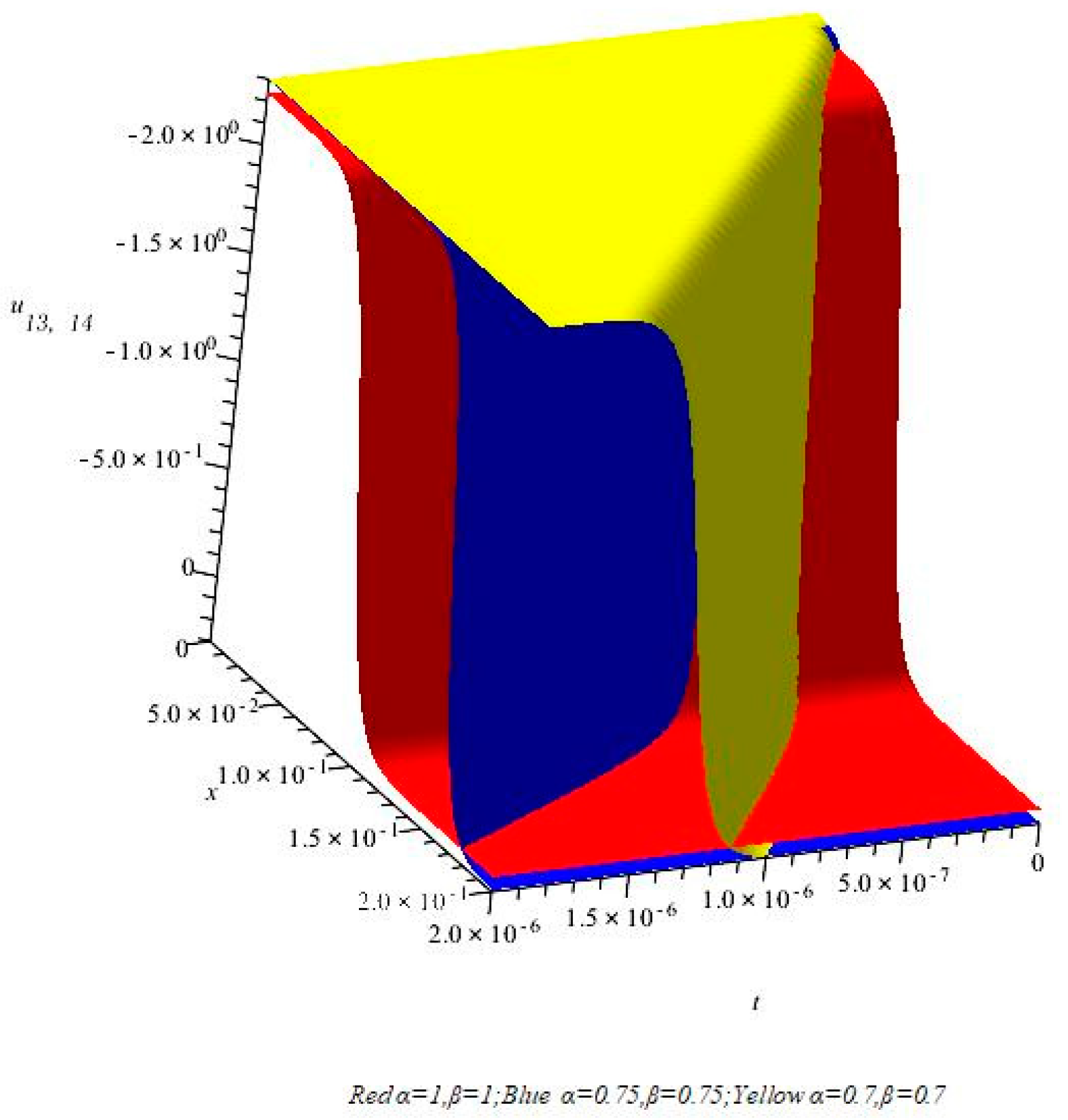
5.2. Numerical Simulation Analysis of u_13,14 and Its Corresponding Fractal Dimension Bell-Shaped Strain Solitary Wave

Considering the rod with a cross-sectional radius R = 0.1 m processed from 35CrMnSi steel, the material parameters of 35CrMnSi steel are taken as

$$E=214.0\mathrm{Gpa},\nu =0.274,\rho {=7600\mathrm{kg}/\mathrm{m}}^3,G=0.5E/(1+\nu )=84.0\mathrm{Gpa},$$

(26)

From the results of the existence analysis of the solution, combined with the Formula (26) and R = 0.14 m, and taking $\beta =1$, $h<-E/8G{R}^2{\nu }^2=-216.5$ is calculated. In the case of $h<0$, from Equations (16) and (11), the fractal dimension wave velocity in Equation (19) is

$$c^{\alpha }=\sqrt{0.5(8G{R}^{2\beta }h{\nu }^2+E)/(4R^{2\beta }h{\nu }^2\rho -\rho )}.$$

(27)

Taking $0<x<0.2,0<t<0.000002,h=-1000,{\xi }_0=-5$, combined with the material parameters in Formula (26), the three-dimensional numerical simulation diagrams of u_13,14 with positive coefficients under different space-time fractal dimensions are drawn, as shown in Figure 1. It can be seen that it is a kink solitary wave. The kink solitary wave rotates with the decrease of the space-time fractal dimension, the waveform is steeper, and the amplitude becomes larger.

For Equation (7), the relation between axial displacement gradient u and axial strain is ${\epsilon }_x=u+0.5u^2$, so the axial nonlinear strain wave function corresponding to solution u_13,14 is

$$\begin{array}{ll}\hfill {\epsilon }_1(x,t)& ={\epsilon }_1(\xi )=-0.5+\frac{12.0h{\tanh }^2\left(2\sqrt{-h}\left(x^{\beta }-{(ct)}^{\alpha }\right)+{\xi }_0\right)}{p_2}\\ & =-0.5+12\frac{2c^{2\alpha }\rho +E}{E}{\tanh }^2\left(\sqrt{\frac{1}{2}\frac{2c^{2\alpha }\rho +E}{R^{2\beta }{\nu }^2\left(-c^{2\alpha }\rho +G\right)}}\left(x^{\beta }-{(ct)}^{\alpha }\right)+{\xi }_0\right),\end{array}$$

(28)

Taking $0<x<0.2,0<t<0.000002,h=-1000,{\xi }_0=-5$, combined with the material parameters in Formula (26), the three-dimensional numerical simulation diagram of fractal dimension strain ${\epsilon }_1(x,t)$ under different space-time fractal dimensions is drawn, as shown in Figure 2. It can be seen that it is a fractal dimension bell-shaped strain solitary wave. As the space-time fractal dimension decreases, the fractal dimension bell-shaped strain solitary wave rotates, the waveform is steeper, and the positive strain amplitude becomes larger. This means that for the rod with a smaller fractal dimension, a higher tensile strength of the material is required when the fractal dimension bell-shaped strain solitary wave propagates in it. In addition, it can be seen from Figure 2 that as the space-time fractal dimension decreases, the fractal dimension of bell-shaped strain solitary wave waveform changes from a solitary waveform to a local periodic form, which indicates that for some wave solutions, the fractal dimension can change the structure of the waveform. In other words, the fractal dimension can modulate the local periodicity of some solitary waves. To illustrate this conclusion more clearly, based on Figure 2, a snapshot of Equation (28) with the change of space-time fractal dimension is given, as shown in Figure 3.

Analysis of ordinary rod. Taking h = −1000, combined with the material parameters in Formula (26), for $\alpha =\beta =1,\alpha =\beta =0.8,\alpha =\beta =0.75$, according to Formula (27), the results of calculating fractal dimension wave velocity are $c^{\alpha }\approx 2720.83,3040.99,3090.39\mathrm{m}/\mathrm{s}$, respectively. For the radius of the thin rod R = 0.14, as the spatial fractal dimension $\beta$ decreases, the fractal dimension radius $R^{\beta }$ gradually increases. It can be concluded that for ordinary rods ($\alpha =\beta =1$), the radius increases, and the nonlinear wave velocity increases. From the expression of Equation (28), the nonlinear wave velocity increases, and the amplitude increases. Combined with Figure 2, it can be seen that the increase in amplitude corresponds to the increase in positive strain amplitude. This means that when the bell-shaped strain solitary wave propagates in an ordinary rod, the larger the radius, the higher the tensile strength of the material.

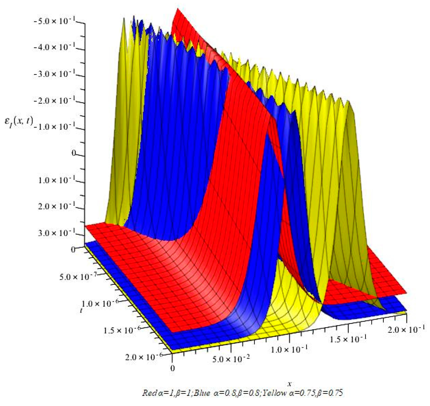
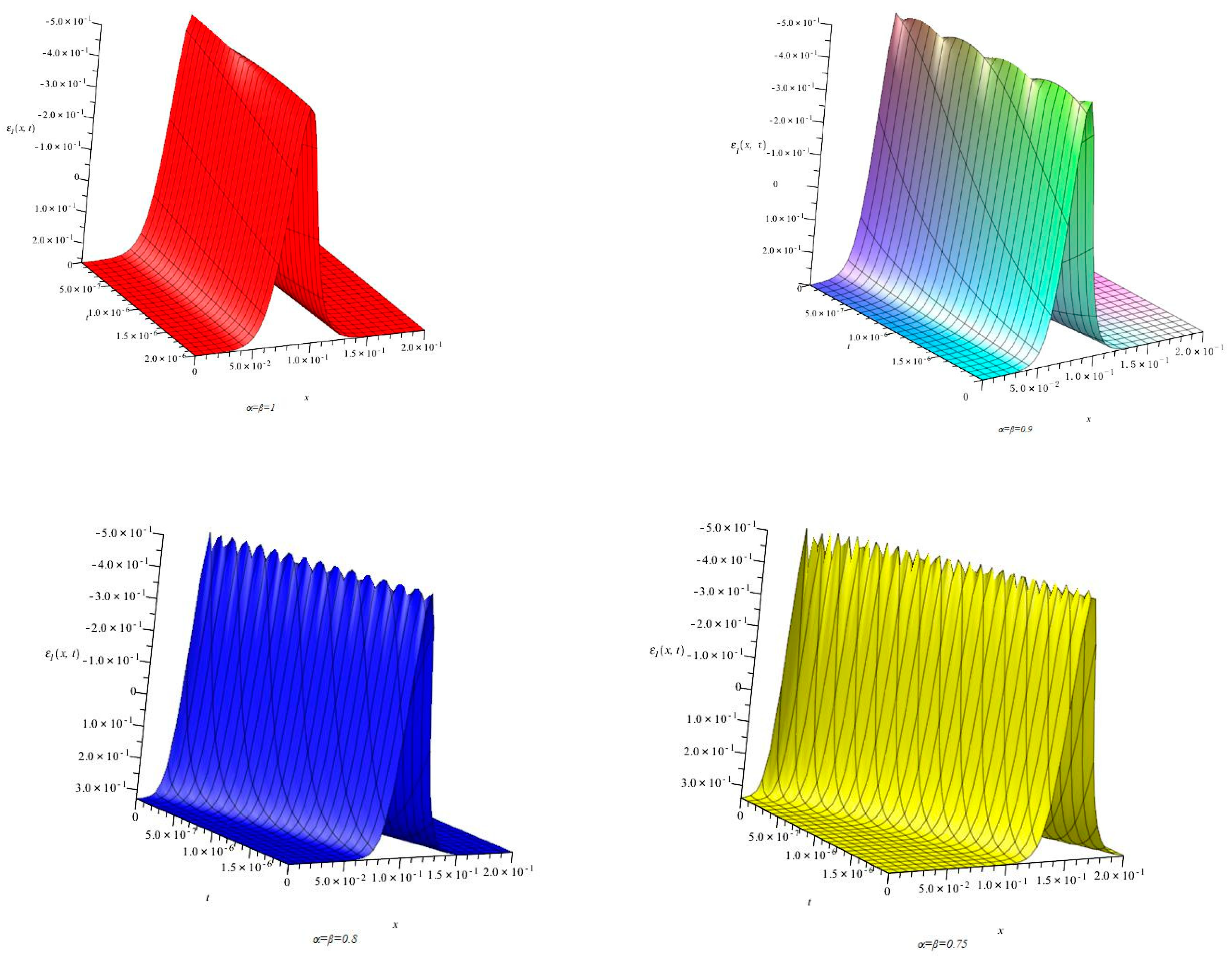
5.3. Numerical Simulation Analysis of Fractal Dimension Strain Blasting Wave Based on u_21,22

Similarly, the fractal dimension wave velocity formula of the exact displacement gradient traveling wave solutions u_21,22 is the same as that of u_13,14, and the axial nonlinear strain wave function corresponding to the solutions u_21,22 is

$$\begin{array}{ll}\hfill {\epsilon }_2(x,t)& ={\epsilon }_2(\xi )=-0.5+\frac{12h{\coth }^2\left(2\sqrt{-h}\left(x^{\beta }-{(ct)}^{\alpha }\right)+{\xi }_0\right)}{p_2}\\ & =-0.5+12\frac{2c^{2\alpha }\rho +E}{E}{\coth }^2\left(\sqrt{\frac{1}{2}\frac{2c^{2\alpha }\rho +E}{R^{2\beta }{\nu }^2\left(-c^{2\alpha }\rho +G\right)}}\left(x^{\beta }-{(ct)}^{\alpha }\right)+{\xi }_0\right),\end{array}$$

(29)

Taking $0<x<0.04,0<t<0.000002,h=-2500,{\xi }_0=-1$, combined with the material parameters in Formula (26), the three-dimensional numerical simulation diagram of fractal dimension strain wave ${\epsilon }_2(x,t)$ under different space-time fractal dimensions is drawn, as shown in Figure 4. It can be seen that it is a fractal dimension strain blasting wave.

In Figure 4, the red represents the strain blasting wave when the space-time fractal dimension index $\alpha =\beta =1$, the blue represents the strain blasting wave when the space-time fractal dimension index $\alpha =\beta =0.85$ and the yellow represents the strain blasting wave when the space-time fractal dimension index $\alpha =\beta =0.75$. It can be seen that with the decrease of the space-time fractal dimension, the fractal dimension strain blasting wave rotates, the waveform is steeper, the wave width is smaller, and the energy is more concentrated. That is to say when the fractal dimension strain blasting wave propagates in the fractal thin rod, the smaller the fractal dimension, the greater the destructive force on the material, and the higher the tensile strength of the material.

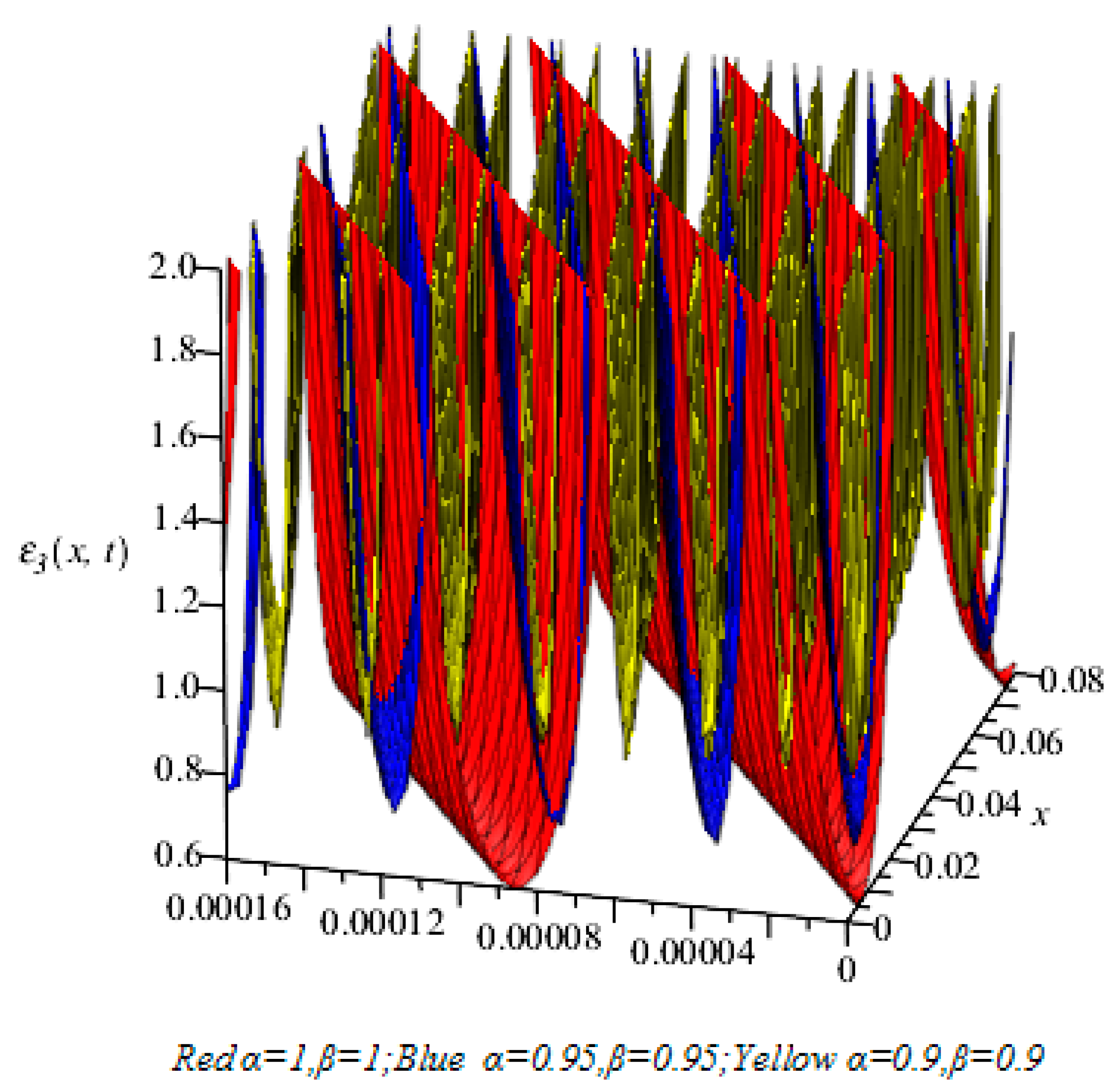
5.4. Numerical Simulation Analysis of Fractal Dimension Strain Periodic Wave Based on u_3,4

It can be seen from Table 1 that for the wave propagation model Equation (7), to make the longitudinal wave propagation model in the fractal thin rod have a displacement gradient periodic wave solution like u_3,4, the parameter h should satisfy $h>E/4G{R}^{2\beta }{\nu }^2$. Taking $\beta =1$, the material parameter data in Formula (26) and $R=0.14m$, $h>E/4G{R}^2{\nu }^2=432.9$ is calculated. In the case of h > 0, from Equations (14) and (11), the fractal dimension wave velocity in Equation (18) is

$$c^{\alpha }=\sqrt{0.5(E-4G{R}^{2\beta }h{\nu }^2)/\left[\rho \left(2R^{2\beta }h{\nu }^2+1\right)\right]}.$$

(30)

Similarly, the axial fractal dimension strain wave function corresponding to u_3,4 is

$${\epsilon }_3(x,t)=-0.5-\frac{12.0h{\csc }^2\left(2\sqrt{h}\left(x^{\beta }-{(ct)}^{\alpha }\right)+{\delta }_0\right)}{p_2}.$$

(31)

Taking $0<x<0.08,0<t<0.00016,h=500,{\xi }_0=-5$, combined with the material parameters in Formula (26), the three-dimensional numerical simulation diagram of fractal dimension strain wave ${\epsilon }_3(x,t)$ under different space-time fractal dimensions is drawn, as shown in Figure 5. It can be seen that it is a fractal dimension strain periodic wave. In Figure 5, the red represents the strain periodic wave when the space-time fractal dimension index $\alpha =\beta =1$, the blue represents the strain periodic wave when the space-time fractal dimension index $\alpha =\beta =0.95$ and the yellow represents the strain periodic wave when the space-time fractal dimension index $\alpha =\beta =0.9$. It can be seen that with the decrease of the space-time fractal dimension, the period of the fractal dimension strain periodic wave becomes smaller, the minimum positive amplitude value increases, the waveform becomes steeper, and the wave width becomes smaller. This means that when the fractal dimension strain periodic wave propagates in the fractal thin rod, the smaller the fractal dimension, the greater the damage to the material and the higher the tensile strength of the material.

6. Conclusions

The model was derived, and its exact solution was obtained. The derivation of the fractal nonlinear propagation model equation of longitudinal wave in rod was completed, and a large number of hyperbolic function, trigonometric function, and rational function forms of exact displacement gradient traveling wave solutions of the equation were obtained. Through the comparative discussion of these solutions and the mechanism analysis of the solution method, it was clarified that the extended (G′/G) expansion method could not only obtain the exact solutions obtained by the (G′/G) expansion method and the (G/G′) expansion method but also obtain new forms of solutions coupled by the exact solutions of the two Riccati equations.

Three existing and independent fractal dimension strain waves are obtained. Under the condition that the real number field and the material parameters are positive, the existence of all the exact displacement gradient solutions was analyzed. It was found that there were three groups of different exact displacement gradient solutions u_13,14, u_21,22, u_3,4, and then the corresponding three fractal dimension strain waves were obtained. They were fractal dimension bell-shaped strain solitary wave, fractal dimension strain burst wave, and fractal dimension strain periodic wave.

The numerical simulation of three kinds of fractal dimension strain waves is studied. As the space-time fractal dimension decreases, the fractal dimension bell-shaped strain solitary wave rotates, the waveform becomes steeper, the positive strain amplitude increases, and the waveform changes from an isolated waveform to a local periodic form. With the decrease of space-time fractal dimension, the fractal dimension strain blasting wave rotates, the waveform is steeper, and the energy is more concentrated. With the decrease of space-time fractal dimension, the period of fractal dimension strain periodic wave becomes smaller, the minimum positive amplitude value increases, the waveform is steeper, and the wave width becomes smaller. These results show that the fractal dimension can modulate the waveform of the longitudinal wave in the functionally graded rod. When the fractal dimension strain wave propagates in the fractal thin rod, the smaller the fractal dimension is, the higher the tensile strength of the material that is required.

The model equation established in this paper is helpful to the further study of the dynamic behavior of rod-shaped mechanical components under high-speed impact or heavy-load impact. In addition, the evolution analysis of strain waves with fractal dimension contributed to the study of the dynamic performance of functionally graded rod-shaped mechanical components. By setting the space-time fractal dimensions $(\alpha ,\beta )$ as functions of coordinates x and t, the evolution of longitudinal waves in rods under variable fractal dimensions can be further studied, which provides a certain reference value for the preparation and dynamic performance study of functionally graded rod-shaped components.

References

1. Minoo, N.; Kamyar, S. Functionally graded materials: A review of fabrication and properties. Appl. Mater. Today 2016, 5, 223–245. [Google Scholar]
2. Barbaros, I.; Yang, Y.; Safaei, B.; Yang, Z.; Qin, Z.; Asmael, M. State-of-the-art review of fabrication, application, and mechanical properties of functionally graded porous nanocomposite materials. Nanotechnol. Rev. 2022, 11, 321–371. [Google Scholar] [CrossRef]
3. Gupta, S.; Bhengra, N. Study of the surface wave vibrations in a functionally graded material layered structure: A WKB method. Math. Mech. Solids 2019, 24, 1204–1220. [Google Scholar] [CrossRef]
4. Kiełczyński, P.; Szalewski, M.; Balcerzak, A.; Wieja, K. Propagation of ultrasonic Love waves in nonhomogeneous elastic functionally graded materials. Ultrasonics 2015, 65, 220–227. [Google Scholar] [CrossRef]
5. Chen, W.Q.; Wang, H.M.; Bao, R.H. On calculating dispersion curves of waves in a functionally graded elastic plat. Compos. Struct. 2007, 81, 233–242. [Google Scholar] [CrossRef]
6. Lee, J.C.; Ahn, S.H. Bulk Density Measurement of Porous Functionally Graded Materials. Int. J. Precis. Eng. Man. 2018, 19, 31–37. [Google Scholar] [CrossRef]
7. Wu, H.L.; Yang, J.; Kitipornchai, S. Mechanical analysis of functionally graded porous structures: A review. Int. J. Struct. Stab. Dyn. 2020, 20, 2041015. [Google Scholar] [CrossRef]
8. Shafiei, N.; Kazemi, M. Buckling analysis on the bidimensional functionally graded porous tapered nano-micscale beams. Aerosp. Sci. Technol. 2017, 66, 1–11. [Google Scholar] [CrossRef]
9. Akbas, S.D. Forced vibration analysis of functionally graded porous deep beams. Compos. Struct. 2018, 186, 293–302. [Google Scholar] [CrossRef]
10. Mesbaha, A.; Belabed, Z.; Amara, K.; Tounsi, A.; Bousahla, A.A.; Bourada, F. Formulation and evaluation a finite element model for free vibration and buckling behaviours of functionally graded porous (FGP) beams. Struct. Eng. Mech. 2023, 86, 291–309. [Google Scholar]
11. Katiyar, V.; Gupta, A.; Tounsi, A. EMicrostructural/geometric imperfection sensitivity on the vibration response of geometrically discontinuous bi-directional functionally graded plates (2D-FGPs) with partial supports by using FEM. Steel Compos. Struct. 2022, 45, 621–640. [Google Scholar]
12. He, J.H. Fractal calculus and its geometrical explanation. Results Phys. 2018, 10, 272–276. [Google Scholar] [CrossRef]
13. He, J.H. A new fractal derivation. Therm. Sci. 2011, 15, 145–147. [Google Scholar] [CrossRef]
14. He, J.H.; Ain, Q.T. New promises and future challenges of fractal calculus from two-scale thermodynamics to fractal variational principle. Therm. Sci. 2020, 24, 659–681. [Google Scholar] [CrossRef]
15. Lin, Y.Q.; Feng, J.W.; Zhang, C.C.; Teng, Y.; Liu, Z.; He, J.H. Air permeability of nanofiber membrane with hierarchical structure. Therm. Sci. 2018, 22, 1637–1643. [Google Scholar]
16. Li, X.X.; Tian, D.; He, C.H.; He, J.H. A fractal modification of the surface coverage model for an electrochemical arsenic sensor. Electrochim. Acta 2019, 296, 491–493. [Google Scholar] [CrossRef]
17. Wang, Q.; Shi, X.; He, J.H.; Li, Z.B. Fractal Calculus and its Application to Explanation of Biomechanism of Polar Bear Hairs. Fractals 2018, 26, 1850086. [Google Scholar] [CrossRef]
18. Wang, Y.; Deng, Q. Fractal derivative Model for Tsunami Travelling. Fractals 2019, 27, 1950017. [Google Scholar] [CrossRef]
19. Yan, W.; An, J.Y. Amplitude-frequency relationship to a fractional Duffing oscillator arising in microphysics and tsunami motion. J. Low Freq. Noise Vib. Act. Control. 2019, 38, 1008–1012. [Google Scholar]
20. Liu, Z.F.; Zhang, S.Y. Three Kinds of Nonlinear Dispersive Waves in Elastic Rods with Finite Deformation. Appl. Math. Mech. 2008, 29, 909–917. [Google Scholar]
21. Liu, J.K.; Wei, W.; Wang, J.B.; Xu, W. Limit behavior of the solution of Caputo-Hadamard fractional stochastic differential equations. Appl. Math. Lett. 2023, 140, 108586. [Google Scholar] [CrossRef]
22. Liu, J.K.; Wei, W.; Xu, W. An averaging principle for stochastic fractional differential equations driven by fBm involving impulses. Fractal. Fract. 2022, 6, 256. [Google Scholar] [CrossRef]
23. Khan, K.; Akba, M.A.; Salam, M.A.; Islam, M.H. A note on enhanced (G’/G)-expansion method in nonlinear physics. Ain. Shams Eng. J. 2014, 5, 877–884. [Google Scholar] [CrossRef] [Green Version]
24. Shahzad, S. New soliton wave structures of nonlinear (4 + 1)-dimensional Fokas dynamical model by using different methods. Alex. Eng. J. 2021, 60, 795–803. [Google Scholar]
25. Ullah, N.; Asjad, M.I.; Awrejcewicz, J.; Muhammad, T.; Baleanu, D. On soliton solutions of fractional-order nonlinear model appears in physical sciences. AIMS Math. 2022, 7, 7421–7440. [Google Scholar] [CrossRef]
26. Jiang, Z.; Zhang, Z.G.; Li, J.J.; Yang, H.W. Analysis of Lie Symmetries with Conservation Laws and Solutions of Generalized (4 + 1)-Dimensional Time-Fractional Fokas Equation. Fractal. Fract. 2022, 6, 108. [Google Scholar] [CrossRef]
27. Hu, X.R.; Lin, S.N.; Wang, L. Integrability, multiple-cosh, lumps and lump-soliton solutions to a (2 + 1)-dimensional generalized breaking soliton equation. Commun. Nonlinear Sci. 2020, 91, 105447. [Google Scholar] [CrossRef]
28. Gardner, C.S.; Greene, J.M.; Kruskal, M.D.; Miura, R.M. Method for solving the Kortweg-de Vries equation. Phys. Rev. Lett. 1967, 19, 1095–1097. [Google Scholar] [CrossRef]
29. Malfliet, W. Solitary wave solutions of nonlinear wave equations. Am. J. Phys. 1992, 60, 650–654. [Google Scholar] [CrossRef]
30. Fan, E.G. Extended tanh-function method and its applications to nonlinear equations. Phys. Lett. A 2000, 277, 212–218. [Google Scholar] [CrossRef]
31. Khuri, S.A. A complex tanh-function method applied to nonlinear equations of Schrödinger typ. Chaos Soliton. Fract. 2004, 20, 1037–1040. [Google Scholar] [CrossRef]
32. Elwakil, S.A.; Labany, S.K.; Zahran, M.A.; Sabry, R. Modified extended tanh-function method and its applications to nonlinear equations. Appl. Math. Comput. 2005, 161, 403–412. [Google Scholar] [CrossRef]
33. Liu, S.K.; Fu, Z.T.; Liu, S.D. Jacobi elliptic function expansion method and periodic wave solutions of nonlinear wave equations. Phys. Lett. A 2001, 289, 69–74. [Google Scholar] [CrossRef]
34. Chen, H.T.; Zhang, H.Q. Improved Jacobi elliptic function method and its applications. Chaos Soliton. Fract. 2003, 15, 585–591. [Google Scholar] [CrossRef]
35. Wang, Q.; Chen, Y.; Zhang, H.Q. A new Jacobi elliptic function rational expansion method and its application to (1 + 1)-dimensional dispersive long wave equation. Chaos Soliton. Fract. 2005, 23, 477–483. [Google Scholar] [CrossRef]
36. Yomba, E. The extended F-expansion method and its application for solving the nonlinear wave, CKGZ, GDS, DS and GZ equations. Phys. Lett. A 2005, 340, 149–160. [Google Scholar] [CrossRef]
37. Kudryashov, N.A.; Loguinova, N.B. Be careful with the exp-function method. Commun. Nonlinear Sci. 2009, 14, 1881–1890. [Google Scholar] [CrossRef] [Green Version]
38. Kudryashov, N.A. One method for finding exact solutions of nonlinear differential equations. Commun. Nonlinear Sci. 2012, 17, 2248–2253. [Google Scholar] [CrossRef] [Green Version]
39. Sirendaoreji. Unified Riccati equation expansion method and its application to two new classes of Benjamin-Bona-Mahony equations. Nonlinear Dynam. 2017, 89, 333–344. [Google Scholar] [CrossRef]
40. Yue, C.; Lu, D.C.; Khater, M.M.A. On explicit wave solutions of the fractional nonlinear DSW system via the modified Khater method. Fractals 2020, 28, 204034. [Google Scholar] [CrossRef]
41. Guo, P.; Tang, R.G.; Sun, X.W. Explicit exact solutions to the wave equation for nonlinear elastic rods. Appl. Math. Mech. 2022, 43, 869–875. [Google Scholar]
42. Wang, M.L.; Li, X.Z.; Zhang, J.L. The (G’/G)-expansion method and travelling wave solutions of nonlinear evolution equations in mathematical physics. Phys. Let. A 2008, 372, 417–423. [Google Scholar] [CrossRef]
43. Ekici, M.; Mirzazadeh, M.; Eslami, M. Solitons and other solutions to Boussinesq equation with power law nonlinearity and dual dispersion. Nonlinear Dynam. 2016, 84, 669–676. [Google Scholar] [CrossRef]
44. Khatuna, M.A.; Arefin, M.A.; Uddin, M.H.; Baleanu, D.; Akbar, M.A.; Inc, M. Explicit wave phenomena to the couple type fractional order nonlinear evolution equations. Results Phys. 2021, 28, 104597. [Google Scholar] [CrossRef]
45. Ali, M.N.; Husnine, S.M.; Saha, A.; Bhowmik, S.K.; Dhawan, S.; Ak, T. Exact solutions, conservation laws, bifurcation of nonlinear and supernonlinear traveling waves for Sharma-Tasso-Olver equation. Nonlinear Dynam. 2018, 94, 1791–1801. [Google Scholar] [CrossRef]
46. Kaplan, M.; Ünsal, Ö.; Bekir, A. Exact solutions of nonlinear Schrödinger equation by using symbolic computation. Math. Method. Appl. Sci. 2016, 39, 2093–2099. [Google Scholar] [CrossRef]
47. Bibi, S.; Mohyud, D.S.T.; Ullah, R.; Ahmed, N.; Khan, U. Exact solutions for STO and (3 + 1)-dimensional KdV-ZK equations using (G’/G2)-expansion method. Results Phys. 2017, 7, 4434–4439. [Google Scholar] [CrossRef]
48. Pang, J.; Bian, C.Q. A new auxiliary equation method for finding travelling wave solutions to KdV equation. Appl. Math. Mech. 2010, 33, 929–936. [Google Scholar] [CrossRef]
49. Fan, K.; Zhou, C.L. Mechanical Solving a Few Fractional Partial Differential Equations and Discussing the Effects of the Fractional Order. Adv. Math. Phys. 2020, 2020, 3758353. [Google Scholar] [CrossRef]
50. Jia, H.X.; Zuo, D.W.; Tian, X.S.; Guo, Z.F. Characteristics of coexisting rogue wave and breather in vector nonlinear Schrödinger system. Appl. Math. Lett. 2023, 136, 108461. [Google Scholar] [CrossRef]
51. Bukhari, M.A.; Barry, O.R.; Vakakis, A.F. Breather propagation and arrest in a strongly nonlinear locally resonant lattice. Mech. Syst. Signal Pr. 2023, 183, 109623. [Google Scholar] [CrossRef]
52. Zhong, W.P.; Yang, Z.P.; Milivoj, B.; Zhong, W.Y. Rogue wave excitations of the (2 + 1)-dimensional nonlinear Zakharov system. Nonlinear Dynam. 2023, 111, 6621–6628. [Google Scholar]
53. Chen, W. Time-space fabric underlying anomalous diffusion. Chaos Soliton. Fract. 2006, 28, 923–929. [Google Scholar]
54. Chen, W.; Liang, Y.J. New methodologies in fractional and fractal derivatives modeling. Chaos Soliton. Fract. 2017, 102, 72–77. [Google Scholar] [CrossRef]
Figure 1. Three-dimensional numerical simulation of kink solitary waves with positive coefficients in Equation (19) under different space-time fractal dimensions.
Fractalfract 07 00586 g001
Figure 2. Three-dimensional numerical simulation of Equation (28) under different space-time fractal dimensions.
Fractalfract 07 00586 g002
Figure 3. Snapshots of soliton solution to local periodic solution of Equation (28) for various values of (α, β).
Fractalfract 07 00586 g003
Figure 4. Three-dimensional numerical simulation of Equation (29) under different space-time fractal dimensions.
Fractalfract 07 00586 g004
Figure 5. Three-dimensional numerical simulation of Equation (31) under different space-time fractal dimensions.
Fractalfract 07 00586 g005