Article

Fractional Transformation-Based Decentralized Robust Control of a Coupled-Tank System for Industrial Applications

1
Department of Mechanical, Mechatronics and Manufacturing Engineering, University of Engineering and Technology Lahore, Faisalabad Campus, Faisalabad 38000, Pakistan
2
School of Industrial Engineering, Pontificia Universidad Católica de Valparaíso, Valparaíso 2362807, Chile
3
Faculty of Natural Sciences and Mathematics, Escuela Superior Politécnica del Litoral ESPOL, Guayaquil 090902, Ecuador
4
Faculty of Engineering, Universidad Espíritu Santo, Samborondón 0901952, Ecuador
5
Department of Electrical, Electronics and Telecommunication Engineering, University of Engineering and Technology Lahore, Faisalabad Campus, Faisalabad 38000, Pakistan
6
Centro de Estudios e Investigaciones Estadísticas, Escuela Superior Politécnica del Litoral ESPOL, Guayaquil 090902, Ecuador
7
Centre of Mathematics, Universidade do Minho, 4710-057 Braga, Portugal
*
Authors to whom correspondence should be addressed.
Fractal Fract. 2023, 7(8), 590; https://doi.org/10.3390/fractalfract7080590
Submission received: 6 June 2023 / Revised: 21 July 2023 / Accepted: 25 July 2023 / Published: 30 July 2023

Abstract

:
Petrochemical and dairy industries, waste management, and paper manufacturing fall under the category of process industries where flow and liquid control are essential. Even when liquids are mixed or chemically treated in interconnected tanks, the fluid and flow should constantly be observed and controlled, especially when dealing with nonlinearity and imperfect plant models. In this study, we propose a nonlinear dynamic multiple-input multiple-output (MIMO) plant model. This model is then transformed through linearization, a technique frequently utilized in the analysis and modeling of fractional processes, and decoupling for decentralized fixed-structure H-infinity robust control design. Simulation tests based on MATLAB and SIMULINK are subsequently executed. Numerous assessments are conducted to evaluate tracking performance, external disturbance rejection, and plant parameter fluctuations to gauge the effectiveness of the proposed model. The objective of this work is to provide a framework that anticipates potential outcomes, paving the way for implementing a reliable controller synthesis for MIMO-connected tanks in real-world scenarios.

1. Introduction

Control of linked tank systems is recognized as a crucial challenge in process industries such as pharmaceuticals, food processing, autonomous liquid dispensing, and other chemical-related sectors [1,2]. The traditional proportional, integral, and derivative (PID) controller, noted for its effectiveness in linear systems and its intuitive user-friendly control, is widely used in these industries [3,4,5,6,7,8]. However, when we have multiple-input multiple-output (MIMO) coupled-tank systems, which are nonlinear in essence, standard control methods typically fail to deliver consistent performance because of nonlinearities, parameter variations, and external disturbances. This is where the importance of a linearization process arises, a process often employed in fractional systems [9]. To address these failures, much approaches have explored nonlinear control strategies for multi-tank systems. Such approaches include controls related to nonlinear sliding modes [8], nonlinear backstepping [10], constrained prediction [11], convolution network [12], and fuzzy methods [13,14,15], which are some of the techniques employed to tackle the challenges posed by these nonlinear systems.
We propose a controller that represents a novel approach and unexplored in the context of two-tank systems. The controller is based on H-infinity ( H ) theory, which enables decentralized control of MIMO systems as well as robust control of single-input single-output (SISO) systems [16,17,18,19,20]. A recent study has also demonstrated the potential of fractional transformation-based intelligent H systems in controlling a direct current servo motor [21]. Nonetheless, fixed-structure H controllers offer a significant advantage over traditional H synthesis methods, as our controller can be designed with specific orders and fixed structures. This allows process industries to utilize traditional PID controllers, which are linear such as the real-time controllers. Nevertheless, traditional techniques are often limited by design objectives such as response speed, disturbance rejection, and robust stability. The complex structure and control bandwidth of MIMO systems impose additional challenges for traditional H control architectures [19].
Our advanced linear robust controller tackles these challenges by providing a solution with a simpler gain structure, PID-like characteristics, sophisticated lead-lag features, and an observer-based architecture. Furthermore, a non-smooth H optimizer in the frequency domain is employed to tune the parameters of the proposed controller [22]. With their inherent robustness and linearity, these controllers are ready for direct deployment.
The objective of the present study is to regulate the liquid level in a MIMO coupled-tank system by manipulating the operation of the water pump within the tanks. To reach this objective, the MIMO nonlinear model is first linearized, and then a decoupled linear model is derived, enabling the decentralized and robust construction of our fixed-structure H controller. Subsequently, a reliable fixed-order robust synthesis tailored for the decoupled MIMO model is introduced, ensuring that the time domain performance remains uncompromised [23]. The robust control toolbox in MATLAB proves to be invaluable in the optimization of the proposed decentralized synthesis architecture. Capable of managing plant nonlinearity, external interferences, and measurement noise simultaneously, our advanced robust controller guarantees consistent liquid levels in the MIMO coupled-tank system, synthesizing apt control signals in response to target liquid levels.
The structure of the article is as follows. Section 2 delves into MIMO modeling of the linked tank system. In Section 3, we describe the decoupling model and proposed controller. Section 4 discusses our results. The conclusions of this work are in Section 5.

2. Modeling

This section describes an in-depth discussion of nonlinear MIMO system.

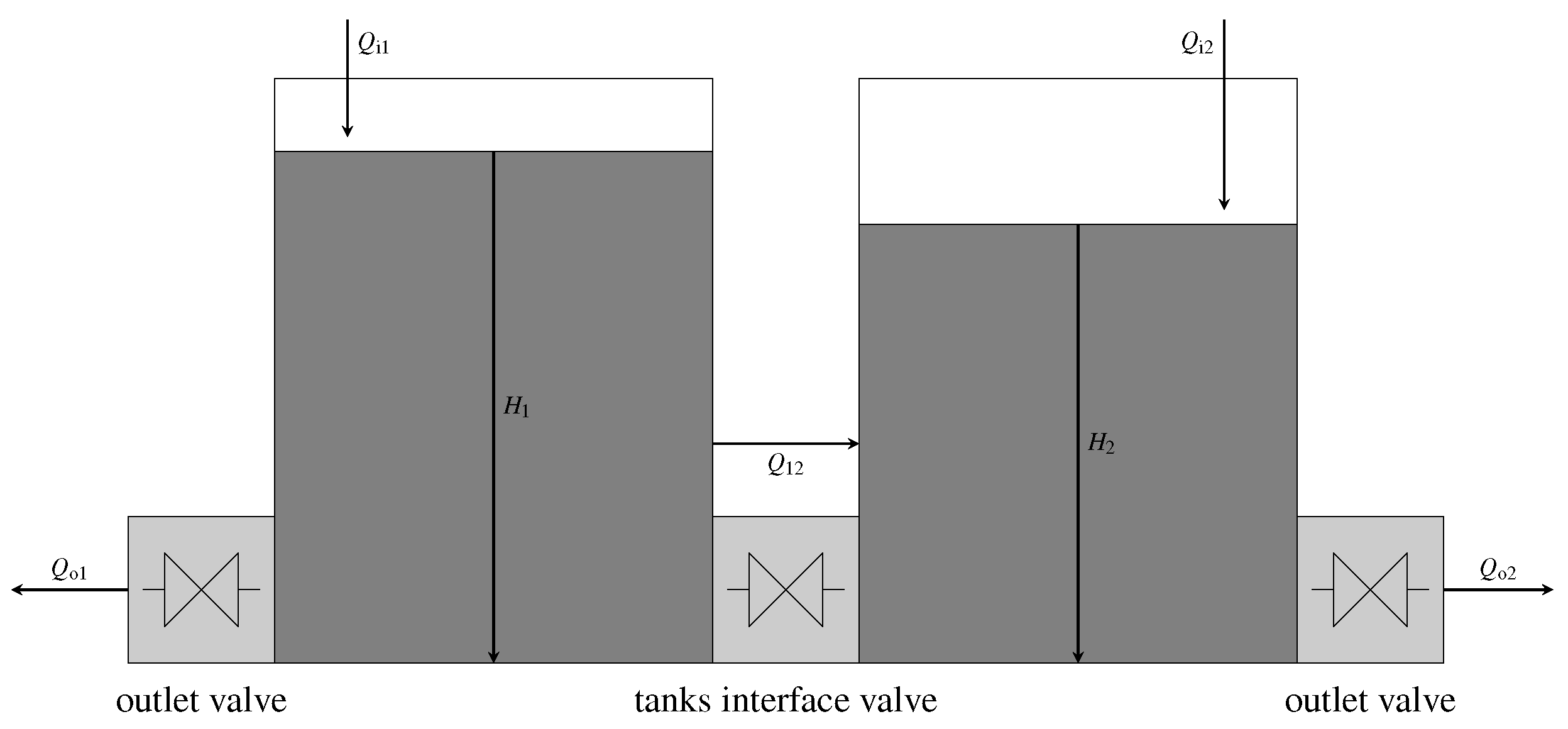
2.1. System’s Description

An industrial coupled-tanks system comprises two tanks interconnected by orifice valves, with electrical valves controlling the input flow into both tanks, and orifice valves regulating the outflow from the tanks. In coupled tanks, there are typically restrictions on the maximum opening of control valves. Such systems exhibit inherent complexity and nonlinearity, presenting challenges for traditional control approaches. Figure 1 illustrates a two-tank system, and Table 1 provides descriptions of the symbols used. The control system’s inputs, Q i 1 and Q i 2 , represent the liquid inflow rates into the tanks via the electrical valves. The control variables, Q o 1 and Q o 2 , indicate the liquid outflow rates through the orifice valves, while H 1 and H 2 represent the MIMO output variables. The orifice flow between the tanks, denoted as Q 12 , facilitates the coupling between the tanks.

2.2. Nonlinear MIMO Mathematical Model

Next, we establish a mathematical model that captures the dynamic behavior of interconnected systems. The nonlinearity and MIMO structure of these systems typify many real-world scenarios. The equations for the dynamic flow balance in tank 1 are
Q i 1 Q o 1 Q 12 = A 1 d d t H 1
and
Q i 2 Q 12 Q o 2 = A 2 d d t H 2 ,
where A 1 , A 2 are the cross-section areas of tanks 1 and 2, respectively; and H 1 , H 2 refer to the baseline or equilibrium liquid levels in tanks 1 and 2, respectively, that is, they represent the static or steady-state levels of the liquid in the absence of any disturbances or inputs.
Using the Bernoulli principle, the formulas stated in (1) and (2) are now converted into nonlinear dynamic equations. The Bernoulli principle, which ignores compressibility and viscosity, relates the steady flow of a flowing liquid to pressure, velocity, and elevation. The fluid flow described by the Bernoulli principle is shown as
P ρ + v 2 2 + g H = c ,
where g is the gravity acceleration, H is the fluid height from the reference point, v is the fluid movement speed, P is the fluid pressure, ρ is the fluid density, and c is a constant.
Applying the Bernoulli principle to a fluid in motion, we get
P 1 ρ + v 1 2 2 + g H 1 = P 2 ρ + v 2 2 2 + g H 2 .
Suppose that v 1 = 0 , P 1 = 0 , and P 2 = 0 . When we solve the equation given in (3), we obtain
v 2 = 2 g ( H 1 H 2 ) .
Then, the equation for coupling flow discharge is formulated as Q 12 = C d a o 12 v 2 , with C d being the discharge coefficient and a o 12 being the coupled orifice cross-section area between tanks 1 and 2, representing the passage that allows flow from one tank to the other. Similarly, we have that
Q o 1 = C d 2 a o 1 2 g H 1 , Q o 2 = C d 3 a o 2 2 g H 2 ,
where a o 1 and a o 2 are the orifice cross-section areas for the outflow from tanks 1 and 2, respectively, which controls the liquid’s discharge from the corresponding tank.
Note that the expressions given in (1) and (2) are changed to
Q i 1 C d 2 a o 1 2 g H 1 C d a o 12 2 g ( H 1 H 2 ) = A d d t H 1
and
Q i 2 + C d a o 12 2 g ( H 1 H 2 ) C d 3 a o 2 2 g H 2 = A d d t H 2 ,
respectively, when the Bernoulli principle has been applied, where A is the cross-section area of tanks 1 and 2. By assuming α 1 = C d a o 12 2 g , α 2 = C d 2 a o 1 2 g , and  α 3 = C d 3 a o 2 2 g , our nonlinear equations are formulated as
Q i 1 α 2 H 1 α 1 H 1 H 2 = A d d t H 1
and
Q i 2 + α 1 H 1 H 2 α 3 H 2 = A d d t H 2 .
These nonlinear equations represent the system’s underlying complexity, paving the way for exploring advanced control strategies in interconnected systems.

2.3. The Perturbed Linearized MIMO Mathematical Model

Next, we aim to develop a linearized model based on perturbations from steady-state conditions, a common approach to simplifying analysis and control design in complex systems.
The liquids in tanks 1–2 and the flow rates, Q i 1 and Q i 2 namely, are assumed to be at steady-state levels. Then, the nonlinear equations adopt the forms given by
Q i 1 + q i 1 α 2 H 1 + h 1 α 1 ( H 1 + h 1 ) ( H 2 + h 2 ) = A d d t ( H 1 + h 1 )
and
Q i 2 + q i 2 + α 1 ( H 1 + h 1 ) ( H 2 + h 2 ) α 3 ( H 2 + h 2 ) = A d d t ( H 2 + h 2 ) ,
if any one of the parameters is slightly altered; where q i 1 and q i 2 are the perturbations in Q i 1 and Q i 2 , respectively; whereas h 1 and h 2 are the perturbations in the liquid levels of tanks 1 and 2, respectively, from their baseline states H 1 and H 2 . In other words, h 1 and h 2 depict how much the liquid levels deviate from their equilibrium states due to disturbances or inputs to the system.
Now, after subtracting and simplifying the nonlinear equations stated in (4) and (5) from the perturbed equations presented in (6) and (7), respectively, we obtain
q i 1 α 2 2 H 1 h 1 α 1 h 1 2 H 1 H 2 + α 1 h 2 2 H 1 H 2 = A d d t H 1
and
q i 2 + α 1 h 1 2 H 1 H 2 α 1 h 2 2 H 1 H 2 α 3 h 2 2 H 2 = A d d t H 2 .
Let
k 1 = α 1 2 H 1 H 2 , k 2 = α 1 2 H 1 H 2 + α 2 2 H 1 , k 3 = α 1 2 H 1 H 2 + α 3 2 H 2 .
Before delving further, it is essential to understand the term LTI, which stands for linear time-invariant, where ‘linear’ means the system obeys superposition principles, and ‘time-invariant’ denotes that the system’s behavior remains consistent over time.
Table 2 provides the system parameters and LTI values for the model presented as
h 1 ˙ h 2 ˙ = k 2 k 1 k 1 k 3 h 1 h 2 + 1 / A 0 0 1 / A q i 1 q i 2 ,
where h ˙ 1 and h ˙ 2 denote the time derivatives of h 1 and h 2 , respectively. In practical terms, h ˙ 1 describes how quickly the variation h 1 is changing over time, indicating the rate at which the liquid level in tank 1 is rising or falling. Similarly, h ˙ 2 represents the rate of change of the variation h 2 , showing how quickly the liquid level in tank 2 is adjusting due to disturbances or inputs. The calculated values from (8) are k 1 = 4.082249 , k 2 = 5.344471 , k 3 = 6.062148 .
Additionally, the system’s MIMO coupled transfer function model is provided below. From input 1 to both outputs, transfer functions are given by
g 11 = 0.25 σ + 1.516 σ 2 + 11.4 σ + 15.67 , g 12 = 1.021 σ 2 + 11.4 s + 15.67 ,
where σ represents the real part of a complex variable in the Laplace domain, commonly used to analyze the dynamics in the frequency domain of control systems and transfer functions. From input 2 to both outputs, transfer functions are formulated as
g 21 = 1.021 σ 2 + 11.4 σ + 15.67 , g 22 = 0.25 σ + 1.334 σ 2 + 11.4 σ + 15.67 .
In the context of MIMO systems, the constants g 11 , g 12 , g 21 , and g 22 represent the transfer functions that define the dynamic interactions between the multiple inputs and outputs. The simulation results for the response of the MIMO LTI model are displayed in Figure 2.
To implement a decentralized control strategy, we opt to split our MIMO model into two distinct SISO systems. Numerous decoupling techniques have been previously documented in scientific publications. In this particular study, we employ a linear decoupling method. We want to introduce an approach for diminishing the interdependency among the control loops by introducing additional decouplers, commonly referred to as controllers, into the multi-loop control system. With this approach, the decoupling matrix D m is designed to minimize interactions across all loops [24]. Consequently, we present the constituent elements for a 2-input-2-output system by means of
D m = d 11 d 12 d 21 d 22 ,
where d 11 = 1 , d 12 = g 12 / g 11 , and  d 21 = g 21 / g 22 , d 22 = 1 are constant elements of the decoupling matrix designed to reduce or eliminate the mentioned interactions, ensuring each control loop operates more independently of the others. The constants d 11 , d 12 , d 21 , d 22 , g 11 , g 12 , g 21 , and g 22 are essential in tuning the system to achieve the desired performance while minimizing unwanted couplings.
After decoupling, a MIMO system may still suffer interactions and perform poorly. The decoupling seeks to counteract the effects of interactions caused by the cross-coupling of system variables [25]. The decoupler’s layout, which was produced using (9), is shown in Figure 3.
The specific values for the decoupler parameters are d 11 = 1 , d 12 = 1.021 / ( 0.25 σ + 1.516 ) , d 21 = 1.021 / ( 0.25 σ + 1.334 ) , and d 22 = 1 . The values make clear that the decoupler described is not in static form, which makes it difficult to implement this decoupling matrix [26]. One strategy for solving this problem is to use static decoupling. The only advantages offered by static decoupling are the constants d 12 and d 21 , whose values are calculated as
d 12 = lim σ 0 1.021 0.25 σ + 1.516 = k 12 k 11
and
d 21 = lim σ 0 1.021 0.25 σ + 1.334 = k 21 k 22 ,
where now k 12 = 1.021 , k 11 = 1.516 , k 21 = 1.021 , and k 22 = 1.334 .
Note that the formulas given in (10) and (11) can be used to determine the two separate SISO systems. Then, the expressions stated in
g 1 = g 11 k 21 k 22 g 12 = 0.25 σ + 0.734559 σ 2 + 11.4 σ + 15.67 ,
g 2 = g 22 k 12 k 11 g 21 = 0.25 σ + 0.646374 2 + 11.4 σ + 15.67
represent the estimated independent transfer functions. The simulation results for the response of the decoupled MIMO LTI model are shown in Figure 4. These results validate the derived linearized models, laying a foundation for exploring more nuanced control design strategies. They hint at the intriguing complexity of the system’s dynamics, subtly underscoring the potential benefits of fractal and fractional approaches in such contexts.

3. Control Design for the Decoupled MIMO System

In this section, we shift our attention towards the construction of control mechanisms for our modeled decoupled MIMO system, which subtly leads to a connection with the multifaceted nature of fractional systems.

3.1. Context

With our decoupled MIMO LTI perturbed model, our primary challenge is to develop a controller capable of producing a suitable transient response and of following the reference input accurately. In this study, we construct and compare three different types of controllers: our H control system, the traditional H , and the PID.
The inflow rates in both tanks serve as control variables, while the liquid levels in each tank represent the measured variables. Performance comparisons among the controllers are made based on their ability to track a reference signal, along with evaluating transient characteristics such as settling time, rising time, steady-state accuracy, and overshoot.

3.2. Traditional PID Design

The traditional PID controllers are widely utilized in the process industries because they are straightforward and have a low cost. For those dynamic models with inherently nonlinear behavior, the PID controllers can occasionally lose some of their effectiveness. Additionally, they do not provide the requisite transient responsiveness and reference tracking parameters. Traditional methods are used to determine the PID parameters. The traditional PID controller is designed utilizing the Zeigler Nicholas pole-zero placement method. The decoupled LTI models of the connected tank system are employed to develop the traditional controllers.
The equations for the PID controller in the frequency and time domains are stated as
U ( s ) = K p + K i 1 s + K d s E ( s )
and
u ( t ) = K p e ( t ) + K i 0 t e ( τ ) d τ + K d d d t e ( t ) ,
where E ( t ) is the Laplace transform of the error in the time domain. This error is the difference between the reference value (or set-point) and the system output. In the frequency domain (s-domain), this error is denoted by E ( s ) . Also, e ( t ) is the error in the time domain, that is, the instantaneous value of the difference between the desired value and the output at a given time t. The PID controller aims to minimize this error by adjusting the system output. Three parameters or gains of the PID controller are the proportional component ( K p ) that acts on the present error, the integral component ( K i ) that acts on the accumulated past errors, and the derivative component ( K d ) that anticipates future errors based on their rate of change.

3.3. Traditional H Controller Design

In this design, both close-loop frequency transfer functions, that is, the complementary sensitivity function, T ( s ) namely, and the sensitivity function, S ( s ) say, are shaped using complicated weights or filters. Note that S ( s ) is the function that transfers frequency between the error signal E ( s ) and the reference input R ( s ) . In contrast, the complementary sensitivity function T ( s ) represents the transfer between the reference input R ( s ) and the output Y ( s ) .
The filters or complex weights have an impact on the shape of closed-loop frequency responses in a traditional H controller’s architecture. Thus, the norm of H , that is, the peak of the objective function, is decreased by choosing appropriate filters or complex weights for S ( s ) and T ( s ) .
The structural complexity and control bandwidth of this traditional H controller is primarily constrained through this H norm. For the purpose of optimizing the controller parameters, the constrained objective function equations are provided as
w S ( s ) S ( s ) 1
and
w T ( s ) T ( s ) 1 ,
where w S ( s ) and w T ( s ) are weighting filters used to shape the frequency responses of the sensitivity S ( s ) and complementary sensitivity T ( s ) , respectively, in the proposed H controller design.
The sensitivity S ( s ) should ideally be as low as feasible over the specified bandwidth range. The bounds on peak specifications, which provide a margin of robustness, are mentioned in (12). In addition to being reliable, the optimum H controller outperforms the traditional PID controller. The mixsynMATLAB tool was employed to implement our H controller.

3.4. Design of Fixed-Structure H Synthesis

The traditional H controller’s order is derived from the combination of the shaping weights and the order of the plant. However, this design complexity in the traditional H controller can limit its practical applications. To address these limitations, this study proposes a decentralized fixed-structure H synthesis.
The robust toolbox of MATLAB is utilized to build the fixed-structure H synthesis. First, the system is represented in the standard form as shown in Figure 5.
Figure 5 illustrates the standard representation of the structured H synthesis, which can be divided into two main sections:
  • Block P ( s ) : represents the non-tunable LTI components of the MIMO system.
  • Block C ( s ) : contains the tunable components diagonally as diag ( C 1 ( s ) , , C N ( s ) ) . Each of these components has a specific structure and is an LTI control element.
The suitable weights w are taken into account to obtain the targeted sensitivity and complementary sensitivity. Then, the control parameters are improved in the frequency domain using non-smooth H optimization [19]. These fixed-structure linear optimal and robust controllers are more practical from an industrial standpoint.
The standard form presented in Figure 5 can be used to configure SISO or MIMO systems, according to the linear robust control [27]. In any control system block diagrams, the block C ( s ) is where all the control elements are arranged and the remaining parts are arranged in the block P ( s ) . In the standard representation, the weight w is composed of disturbances, commands, and external noise. Consider the partition formulated as
z y = P w u = p 11 p 12 p 21 p 22 w u ,
where z is composed of error signals, while the closed loop optimal objective function from w to z is given by a linear rational transformation stated as
T w z = F LTI ( P , C ) = p 11 + p 12 C ( I 2 p 22 C ) 1 p 21 ,
where T w z denotes the closed-loop transfer function from w to z; F LTI ( P , C ) describes the relationship between the process and controller; and I 2 is the identity matrix of orden 2.
Note that the fixed-order linear structure controller is formulated as
C j ( s ) = K p + K i s + K d s T f s + 1 , j { 1 , , M } ,
where M is the total number of distinct specifications or scenarios being considered in the controller design. The suggested controller parameters are optimized via non-smooth H optimization, where, as mentioned, K p is the proportional gain, K i is the integral gain, T f is the first order derivative filter, and K d is the derivative gain coefficient.
Critical design specifications, including disturbance rejection, control bandwidth, and high stability margins, are encapsulated as
w j ( s ) S j ( s ) 1 , w j ( s ) T j ( s ) 1 , j { 1 , , M } .
The H norm stated in H ( s ) = F LTI ( P ( s ) , diag ( C 1 ( s ) , , C N ( s ) ) ) is minimized to satisfy the desired conditions.
The optimization process initiates with randomly generated parameter values and iteratively refines until optimal values are achieved. The results and comparisons are discussed in Section 4, which also presents the optimized controller parameters. The optimized parameter values of the proposed controller are provided in Table 3.

4. Performance Analysis and Discussion

This section evaluates the proposed decentralized control approach for the MIMO-coupled tank system against traditional H and PID controllers, focusing on transient response and command tracking. Precise tracking of desired signals remains a prominent challenge in industries.

4.1. Context

Despite the affordability and simplicity of traditional PID controllers making them a staple in process industries, they sometimes falter, especially when faced with nonlinear system dynamics. In addition, traditional H controllers ensure robust performance, but they are marred by their intricate structure, making them less practical for some applications. The proposed fixed-order H controller strikes a balance, offering dependable performance with a simpler implementation. A distinctive benefit of this synthesis is the flexibility it offers in design. The controller effectively shapes the sensitivity S ( s ) and complementary sensitivity T ( s ) , uninfluenced by complex higher-order weights, contrasting the more intricate standard H controllers.

4.2. Results and Discussion

The optimal parameters for the decentralized control of MIMO-coupled tank systems were depicted in Table 3, and the corresponding expressions for these controllers are provided as
A h 1 = 0.01 0 0 2.28600 1.8680 1.3870 0 4 0 , B h 1 = 4.091 0 0 , C h 1 = 894100 7.2990 54210 , D h 1 = 0 , A h 2 = 0.01 0 0 2.52200 2.0590 1.3440 0 4 0 , B h 2 = 4.087 0 0 , C h 2 = 987400 8.0580 52610 , D h 2 = 0 .
Before proceeding, it is important to clarify a particular aspect of Table 3, namely the negative values of the derivative gain, K d . These values are not errors but a direct result of the optimization process in the fixed-structure H controller design.
After determining the optimized parameters, the resulting controllers are represented in Table 3. These controllers provide the state-space structure of traditional H controllers for decentralized tracking of h 1 and h 2 , respectively. This specific structure is pivotal for the effectiveness of decentralized control and directly contributes to the optimized performance we observe.
While uncommon and negative derivative gains can be part of a balanced solution minimizing an error criterion, such values might pose practical implementation challenges due to the potential phase addition and destabilizing effects. These negative K d values could be problematic in a real-world application. Furthermore, fine-tuning or constraints in the optimization process may be introduced to ensure non-negative derivative gains. Nevertheless, this might deviate the system’s performance from the optimal results obtained for the controllers presented here. These controllers provide the state-space structure of traditional H controllers for decentralized tracking of h 1 and h 2 , respectively.
The comparison in terms of transient definition and commanded tracking among three controllers is shown in Figure 6 and Figure 7. Table 4 presents a comparison based on transient parameters such as steady-state accuracy, percentage overshoot, rising time, and settling time. It can be seen from Table 4 that both H controllers have no overshoot in the transient response, while the traditional PID controller exhibits a significant overshoot in the response.
Compared to the traditional PID controller, the traditional H controller delivers robust performance but with a somewhat slower rise time. In contrast, the proposed fixed-structure H controller shows robust performance across all tested parameters. The response comparison for step disturbance for all three controllers is shown in Figure 8. From this figure, note that the proposed fixed-structure H synthesis provides fast and robust step disturbance rejection as compared to other traditional controllers. The proposed fixed-structure H controller also gives a robust performance in the presence of parameter uncertainty. The performance of the proposed controller is evaluated for a wide range of parameter values and the results are shown in Figure 9.

5. Conclusions

In this research, we proposed a decentralized intelligent robust controller for a MIMO coupled-tank system. This system has been a longstanding challenge in process industries, and numerous control strategies have been previously employed to manage it, such as nonlinear sliding mode control, nonlinear backstepping control, predictive constrained control, convolution network control, and fuzzy control. However, as demonstrated in Table 4, our proposed controller, based on H theory, has shown to outperform traditional H and PID controllers in terms of transient requirements.
The fixed order and fixed structure of the proposed controller are additional advantages. These characteristics highlight the pertinence of our study in the context of fractal and fractional systems, where the complexity often resides in the intricate structure and variable order of the controllers. In contrast to traditional H synthesis, where the order increases when dealing with complex filter transfer functions, our proposed controller maintains a fixed-order, an advantage previously demonstrated in the control of a direct current servo motor. The proposed controller is decentralized robust linear and utilizes intelligent non-smooth H optimization for its parameters. Its straightforward gains or optimized PID-based structure makes it practical and easy to use. Despite the complex structure and control bandwidth challenges associated with MIMO systems, our proposed linear robust controller has shown, through comparative simulation results, to be robust against parameter changes.
Future work should consider addressing the issue of actuator saturation, which is critical in process industries. A potential solution could be the incorporation of a strategy related to anti-integral windup in the design of a decentralized fixed-structure H controller. To ensure stability in the presence of actuator saturation, additional simulation results can be obtained prior to real-time implementation, ensuring no risk of systemic instability or damage. Furthermore, while our study provided promising simulation results, future research should also focus on real-world verification to further substantiate the efficacy of the proposed controller.

Author Contributions

Conceptualization, M.Z.U.R., V.L., C.M.-B., A.W., X.C. and C.C.; Methodology, M.Z.U.R., V.L., A.G., C.M.-B., A.W., X.C. and C.C.; Formal analysis, M.Z.U.R., V.L., A.G., A.W., X.C. and C.C.; Investigation, M.Z.U.R., V.L., A.G., C.M.-B., A.W. and C.C.; Data curation, M.Z.U.R.; Writing—original draft, M.Z.U.R., A.G., C.M.-B., A.W. and X.C.; Writing—review & editing, V.L. and C.C. All authors have read and agreed to the published version of the manuscript.

Funding

This research was partially funded by FONDECYT grant number 1200525 (V.L.) from the National Agency for Research and Development (ANID) of the Chilean government under the Ministry of Science, Technology, Knowledge, and Innovation; and by Portuguese funds through the CMAT—Research Centre of Mathematics of University of Minho—within projects UIDB/00013/2020 and UIDP/00013/2020 (C.C.).

Institutional Review Board Statement

Not applicable.

Informed Consent Statement

Not applicable.

Data Availability Statement

Not applicable.

Acknowledgments

The authors would also like to thank the Editors and four Reviewers for their constructive comments which led to improve the presentation of the manuscript.

Conflicts of Interest

The authors declare no conflict of interest.

References

  1. Singh, A.P.; Mukherjee, S.; Nikolaou, M. Debottlenecking level control for tanks in series. J. Process Control 2014, 24, 158–171. [Google Scholar] [CrossRef]
  2. Antimisiaris, S.G.; Kallinteri, P.; Fatouros, D.G. Liposomes and drug delivery. In Pharmaceutical Manufacturing Handbook: Production and Processes; Wiley: Hoboken, NJ, USA, 2008; pp. 443–507. [Google Scholar]
  3. Saad, M.; Albagul, A.; Abueejela, Y. Performance Comparison between PI and MRAC for Coupled-Tank System. J. Autom. Control Eng. 2014, 2, 316–321. [Google Scholar] [CrossRef] [Green Version]
  4. Tepljakov, A.; Petlenkov, E.; Belikov, J.; Halas, M. Design and implementation of fractional-order PID controllers for a fluid tank system. In Proceedings of the 2013 American Control Conference, Washington, DC, USA, 17–19 June 2013; pp. 1777–1782. [Google Scholar]
  5. Jaafar, H.I.; Yuslinda, S.; Selamat, N.; Mohd Aras, M.S.; Rashid, M.A.Z. Development of PID Controller for Controlling Desired Level of Coupled Tank System. Int. J. Innov. Technol. Explor. Eng. 2014, 3, 32–36. [Google Scholar]
  6. Visioli, A. A new design for a PID plus feed forward controller. J. Process Control 2004, 14, 457–463. [Google Scholar] [CrossRef]
  7. Wu, K.-L.; Yu, C.-C.; Cheng, Y.-C. A two degree of freedom level control. J. Process Control 2001, 11, 311–319. [Google Scholar] [CrossRef]
  8. Khan, M.K.; Spurgeon, S.K. Robust MIMO water level control in interconnected twin-tanks using second order sliding mode control. Control Eng. Pract. 2006, 14, 375–386. [Google Scholar] [CrossRef]
  9. Milev, M.; Zlatev, S. A Note about Stability of Fractional Retarded Linear Systems with Distributed Delays. Int. J. Pure Appl. Math. 2017, 115, 873–881. [Google Scholar] [CrossRef] [Green Version]
  10. Pan, H.; Wong, H.; Kapila, V.; de Queiroz, M.S. Experimental validation of a nonlinear back stepping liquid level controller for a state coupled two tank system. Control Eng. Pract. 2005, 13, 27–40. [Google Scholar] [CrossRef]
  11. Poulsen, N.K.; Kouvaritakis, B.; Cannon, M. Constrained predictive control and its application to a coupled-tanks apparatus. Int. J. Control 2001, 74, 552–564. [Google Scholar] [CrossRef]
  12. Murray-Smith, D.; Kocijan, J.; Gong, M. A signal convolution method for estimation of controller parameter sensitivity functions for tuning of feedback control systems by an iterative process. Control Eng. Pract. 2003, 11, 1087–1094. [Google Scholar] [CrossRef]
  13. Rojas, I.; Anguita, M.; Pomares, H.; Prieto, A. Analysis and electronic implementation of a fuzzy system for the control of a liquid tank. In Proceedings of the 6th International Fuzzy Systems Conference, Barcelona, Spain, 5 July 1997. [Google Scholar]
  14. Ghwanmeh, S.; Jones, K.; Williams, D. Performance Evaluation of an On-Line Self-Learning Fuzzy Logic Controller Applied to Non-Linear Processes. IFAC Proc. Vol. 1997, 30, 245–250. [Google Scholar] [CrossRef]
  15. Muftah, M.N.; Faudzi, A.A.M.; Sahlan, S.; Mohamaddan, S. Fuzzy Fractional Order PID Tuned via PSO for a Pneumatic Actuator with Ball Beam (PABB) System. Fractal Fract. 2023, 7, 416. [Google Scholar] [CrossRef]
  16. Doyle, J.; Glover, K.; Khargonekar, P.P.; Francis, B.A. State-space solutions to standard H2 and H1 control problems. IEEE Trans. Autom. Control 1989, 34, 831–847. [Google Scholar] [CrossRef]
  17. McFarlane, D.; Glover, K. A loop shaping design procedure using H1 synthesis. IEEE Trans. Autom. Control 1992, 37, 759–769. [Google Scholar] [CrossRef]
  18. Zhou, K.; Doyle, J.C.; Glover, K. Robust and Optimal Control; Prentice Hall: New York, NY, USA, 1996. [Google Scholar]
  19. Gahinet, P.; Apkarian, P. Decentralized and fixed-structure H control in MATLAB. In Proceedings of the IEEE Conference on Decision and Control and European Control Conference, Orlando, FL, USA, 12–15 December 2011. [Google Scholar]
  20. Albalawi, H.; Bakeer, A.; Zaid, S.A.; Aggoune, E.-H.; Ayaz, M.; Bensenouci, A.; Eisa, A. Fractional-order model-free predictive control for voltage source inverters. Fractal Fract. 2023, 7, 433. [Google Scholar] [CrossRef]
  21. Rahman, M.Z.U.; Leiva, V.; Martin-Barreiro, C.; Mahmood, I.; Usman, M.; Rizwan, M. Fractional transformation-based intelligent H-infinity controller of a direct current servo motor. Fractal Fract. 2022, 7, 29. [Google Scholar] [CrossRef]
  22. Apkarian, P.; Noll, D. Non-smooth H synthesis. IEEE Trans. Autom. Control 2006, 51, 71–86. [Google Scholar] [CrossRef] [Green Version]
  23. Apkarian, P.; Bompart, V.; Noll, D. Non-smooth structured control design with application to PID loop-shaping of a process. Int. J. Robust Nonlinear Control 2007, 17, 1320–1342. [Google Scholar] [CrossRef] [Green Version]
  24. Vázquez, F.; Morilla, F. Tuning Decentralized Pid Controllers for Mimo Systems with Decouplers. IFAC Proc. Vol. 2002, 35, 349–354. [Google Scholar] [CrossRef]
  25. Sanda Florentina, F. Decoupling in distillation. J. Control Eng. Appl. Inform. 2006, 7, 10–19. [Google Scholar]
  26. Mashhood, A.; Ali, A.; Choudhry, M.A. Fixed-structure H controller design for two-rotor aerodynamical system. Arab. J. Sci. Eng. 2016, 4, 3619–3630. [Google Scholar]
  27. Green, M.; Limebeer, D.J.N. Linear Robust Control; Courier Corporation: North Chelmsford, MA, USA, 2012. [Google Scholar]
Figure 1. Industrial MIMO coupled tank system.
Fractalfract 07 00590 g001
Figure 2. Coupled MIMO LTI model step response.
Fractalfract 07 00590 g002
Figure 3. Decoupled layout for MIMO process, where r 1 , r 2 are the desired responses of liquid height in tanks 1 and 2, whereas G c 1 and G c 2 are decentralized controllers for h 1 and h 2 , respectively.
Fractalfract 07 00590 g003
Figure 4. Decoupled MIMO LTI model step response.
Fractalfract 07 00590 g004
Figure 5. Structured H synthesis in standard representation, where C, P, u, w, and z are earlier defined, while v is the error signal for the SISO system, v is the input to the controller. We use v as a general representation in this figure and this is defined in as v ( t ) = r ( t ) y ( t ) = e ( t ) , with r ( t ) being the reference value, y ( t ) being the true output, and e ( t ) being the error.
Fractalfract 07 00590 g005
Figure 6. Step response for the decentralized control of liquid level h 1 .
Fractalfract 07 00590 g006
Figure 7. Step response for the decentralized control of liquid level h 2 .
Fractalfract 07 00590 g007
Figure 8. Comparison of controllers for step disturbance response in liquid level h 2 .
Fractalfract 07 00590 g008
Figure 9. Performance of the proposed controller for (top) open loop step response with parameters uncertainty in liquid level h 2 and (bottom) step input tracking.
Fractalfract 07 00590 g009
Table 1. Description of notations.
NotationDefinition
Q i 1 Flow index/control input for tank 1
Q i 2 Flow index/control input for tank 2
H 1 Height (liquid) in tank 1
H 2 Height (liquid) in tank 2
Q o 1 Outflow rate through tank 1’s orifice valve
Q o 2 Outflow rate through tank 2’s orifice valve
Q 12 Coupling flow rate between tanks 1 and 2 through orifice valve
ACross-section area of each tank
Table 2. Extended couple tank system’s parameters and values.
NameExpressionValue
Cross-section of tanks 1 and 2A 4 m 2
Discharge coefficients C d , C d 2 , C d 3 1, 0.5, 0.5
Cross sections of an orifice valve a o 12 , a o 1 , a o 2 1 cm 2
Gravitational accelerationg 9.8 m / s 2
SensorIdeal1
Liquid levels offset H 1 , H 2 0.5  m, 0.2  m
Dynamics constant 1 k 1 4.082249
Dynamics constant 2 k 2 5.344471
Dynamics constant 3 k 3 6.062148
Table 3. Optimized parameters of decentralized fixed-structure H controller.
Symbols   DescriptionValues for h 1 TrackingValues for h 2 Tracking
K p Proportional gain67304210
K i Integral gain32303660
K d Derivative gain−9750−8580
T f 1st order filter coefficient1.642.44
Table 4. Controllers performance evaluation for h 2 .
ControllerRise Time
(s)
Settling Time
(s)
Over-Shoot
(%)
Steady-State ErrorController Order
Traditional H 0.04480.080100%Third
Fixed-structure H 0.01310.024900%Second
PID0.02680.145110.32890.1033Second
Disclaimer/Publisher’s Note: The statements, opinions and data contained in all publications are solely those of the individual author(s) and contributor(s) and not of MDPI and/or the editor(s). MDPI and/or the editor(s) disclaim responsibility for any injury to people or property resulting from any ideas, methods, instructions or products referred to in the content.

