Qualitative Analysis for Solving a Fractional Integro-Differential Equation of Hyperbolic Type with Numerical Treatment Using the Lerch Matrix Collocation Method
Abstract
:1. Introduction
2. Preliminaries
- for .
- The operator equation has a solution for , or
- The setis unbounded for .
3. Analysis for Existence and Uniqueness Solutions for the Model (1)–(2)
4. Lerch Matrix Collocation Method
4.1. Numerical Solution of Problem (1)–(2) Using LMC Method
4.2. Error Analysis
4.3. Convergence Analysis of the Problem (1)–(2)
5. Numerical Examples
Comparison of the Findings
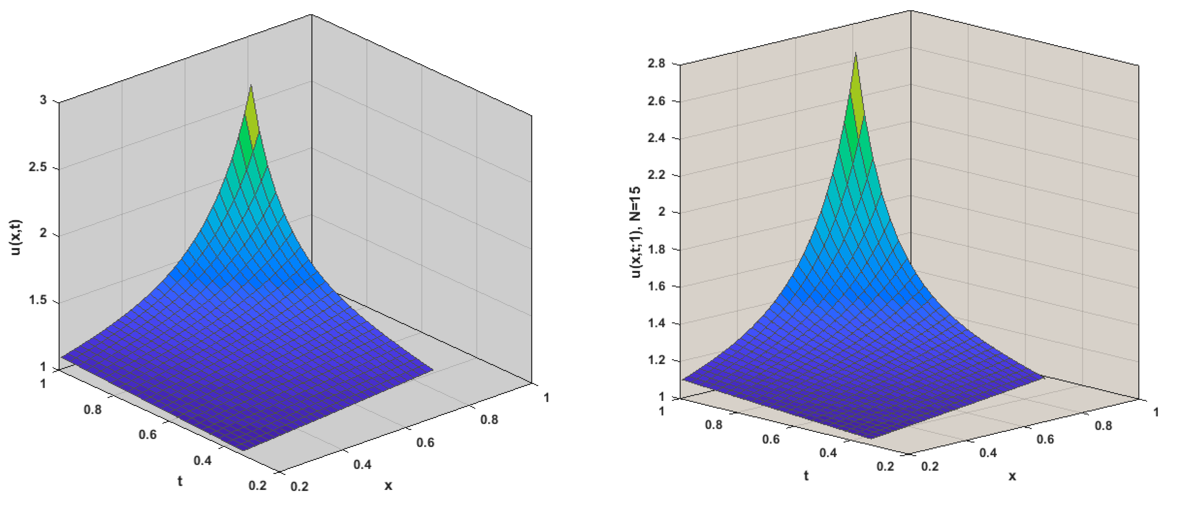
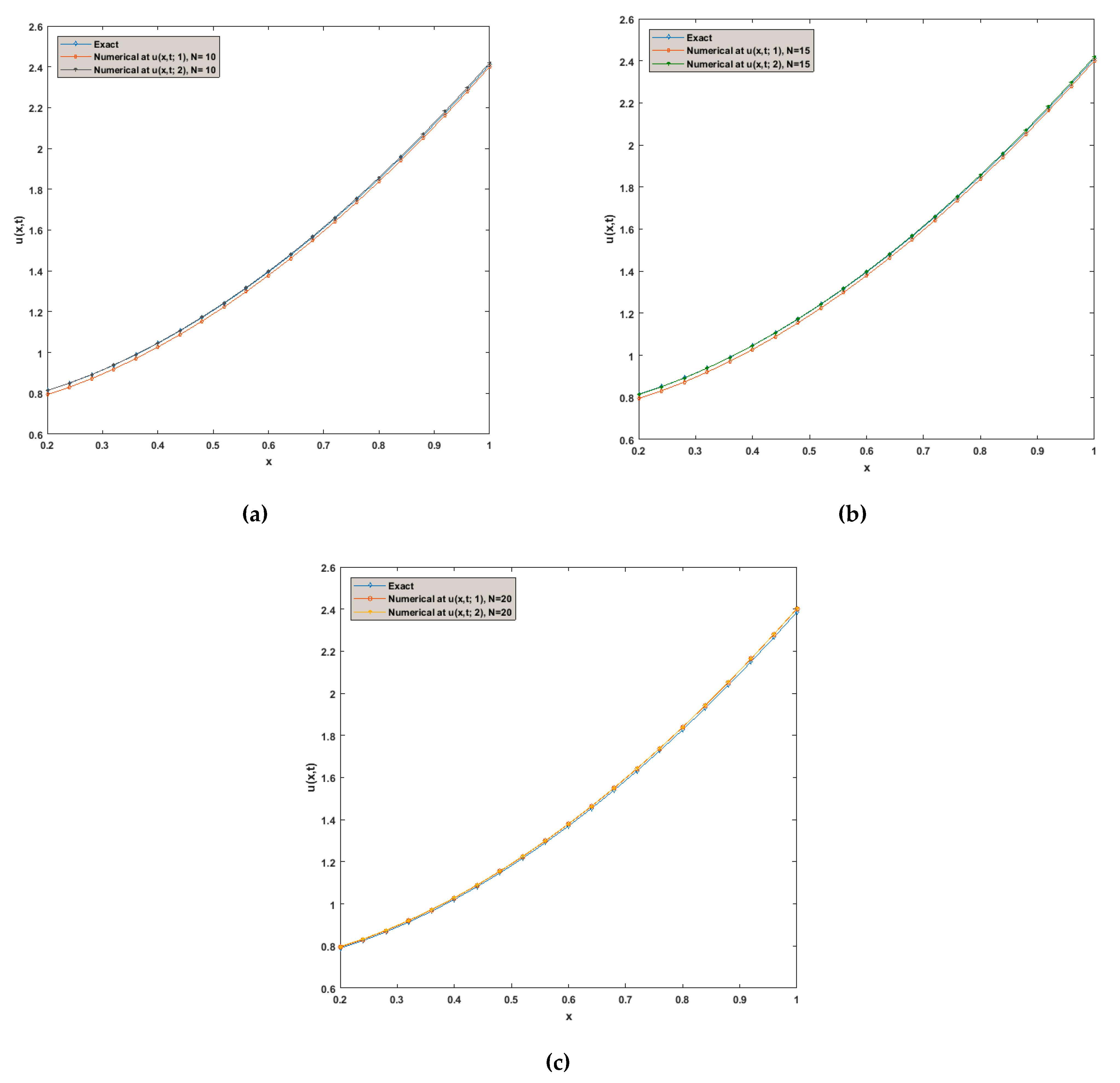
- Based on Example 1, the variation among exact solutions and approximate solutions for distinct values of N is computed according to Table 1. From the absolute errors, we noticed the following:
- For we have:
| λ = 1 | λ = 2 | |||||
| x | t | Abs. Error | x | t | Abs. Error | |
| Highest Error | 0.2 | 0.66 | 2.55 × 10⁻⁸ | 0.2 | 0.33 | 1.45 × 10⁻⁸ |
| Lowest Error | 0.8 | 0.99 | 4.24 × 10⁻¹² | 0.8 | 0.99 | 2.53 × 10⁻¹² |
- For we have:
| λ = 1 | λ = 2 | |||||
| x | t | Abs. Error | x | t | Abs. Error | |
| Highest Error | 0.2 | 0.33 | 2.24 × 10⁻⁸ | 0.2 | 0.33 | 6.11 × 10⁻⁸ |
| Lowest Error | 0.2 | 0.99 | 7.11 × 10⁻¹¹ | 0.4 | 0.99 | 7.17 × 10⁻¹² |
- For we have:
| λ = 1 | λ = 2 | |||||
| x | t | Abs. Error | x | t | Abs. Error | |
| Highest Error | 0.2 | 0.66 | 1.42 × 10⁻⁸ | 0.4 | 0.33 | 1.89 × 10⁻⁸ |
| Lowest Error | 0.8 | 0.99 | 9.95 × 10⁻¹² | 0.8 | 0.66 | 8.91 × 10⁻¹² |
- 2.
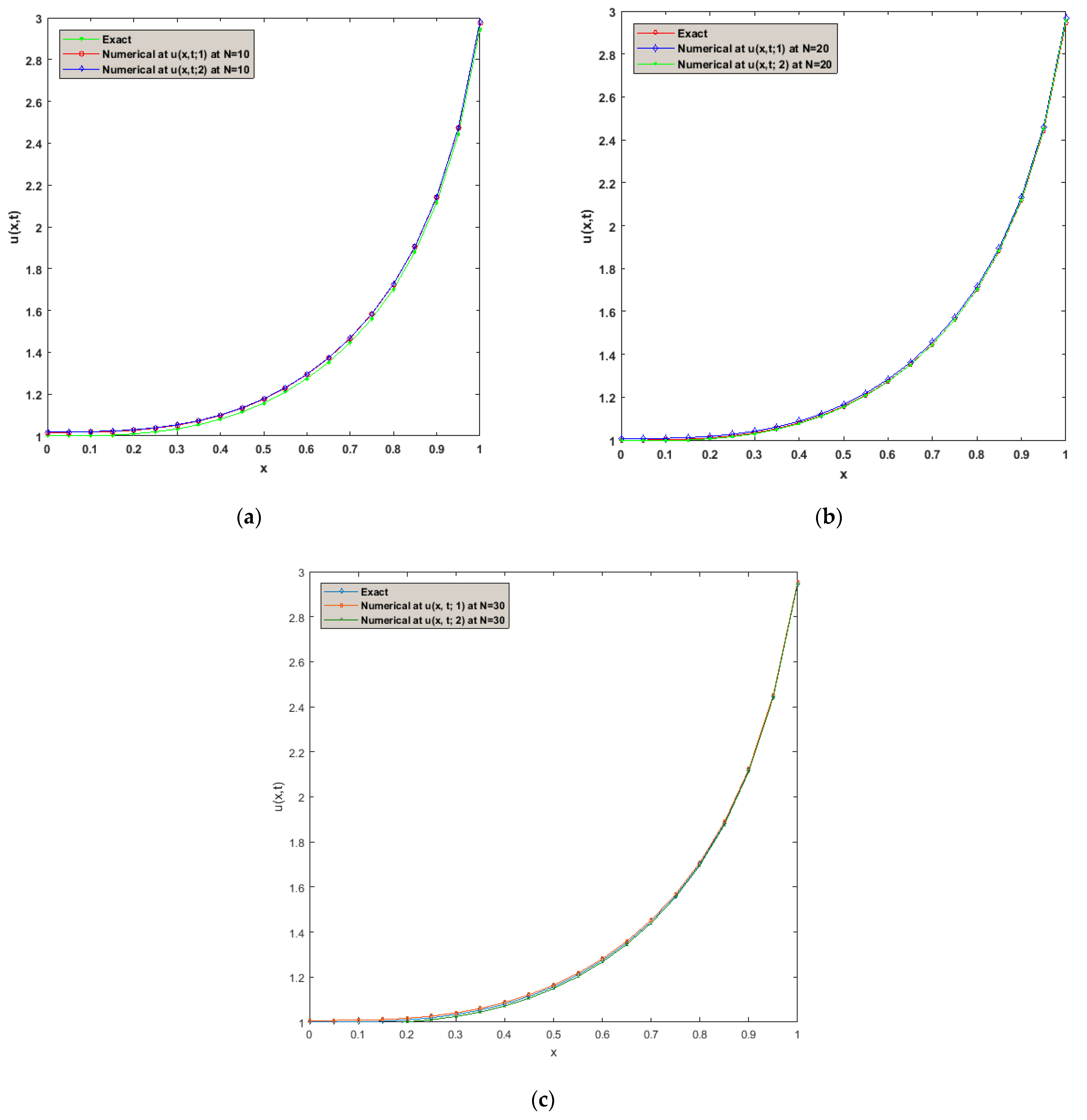
- According to Example 2, for different values of N, the difference between exact solutions and approximate solutions was displayed in Table 2. We reached the following results from the absolute errors:
- For we have:
| λ = 1 | λ = 2 | |||||
| x | t | Abs. Error | x | t | Abs. Error | |
| Highest Error | 0.4 | 0.99 | 2.55 × 10⁻¹⁰ | 0.6 | 0.33 | 2.06 × 10⁻¹⁰ |
| Lowest Error | 0.4 | 0.99 | 8.93 × 10⁻¹² | 0.8 | 0.66 | 5.04 × 10⁻¹³ |
- For , we have:
| λ = 1 | λ = 2 | |||||
| x | t | Abs. Error | x | t | Abs. Error | |
| Highest Error | 0.6 | 0.66 | 4.26 × 10⁻¹⁰ | 0.2 | 0.33 | 1.35 × 10⁻⁸ |
| Lowest Error | 0.4 | 0.99 | 3.53 × 10⁻¹² | 0.8 | 0.99 | 7.68 × 10⁻¹³ |
- For we have:
| λ = 1 | λ = 2 | |||||
| x | t | Abs. Error | x | t | Abs. Error | |
| Highest Error | 0.2 | 0.33 | 3.23 × 10⁻¹¹ | 0.2 | 0.66 | 1.24 × 10⁻⁸ |
| Lowest Error | 0.8 | 0.99 | 6.13 × 10⁻¹³ | 0.8 | 0.99 | 9.08 × 10⁻¹⁴ |
6. Conclusions
Future Work
Author Contributions
Funding
Data Availability Statement
Conflicts of Interest
References
- Petras, I. (Ed.) Handbook of Fractional Calculus with Applications; De Gruyter: Berlin, Germany, 2019. [Google Scholar] [CrossRef]
- Patil, J.; Chaudhari, A.; Mohammed, A.B.D.O.; Hardan, B. Upper and lower solution method for positive solution of generalized Caputo fractional differential equations. Adv. Theory Nonlinear Anal. Its Appl. 2020, 4, 279–291. [Google Scholar] [CrossRef]
- El-borai, M.M.; ElSayed, W.G.; Abdou, M.A.; Taha, E.M. On the Fractional Optimal Control Problem with Free End Point. Am. J. Theor. Appl. Stat. 2017, 6, 46–50. [Google Scholar]
- Baitiche, Z.; Guerbati, K.; Benchohra, M.; Zhou, Y. Solvability of Fractional Multi-Point BVP with Nonlinear Growth at Resonance. J. Contemp. Math. Anal. 2020, 55, 126–142. [Google Scholar] [CrossRef]
- Abdo, M.S.; Ibrahim, A.G.; Panchal, S.K. Nonlinear implicit fractional differential equation involving-Caputo fractional derivative. Proc. Jangjeon Math. Soc. 2019, 22, 387–400. [Google Scholar]
- Zhou, Y. Attractivity for fractional differential equations in Banach space. Appl. Math. Lett. 2018, 75, 1–16. [Google Scholar] [CrossRef]
- Zhou, Y. Basic Theory of Fractional Differential Equations; World Scientific: Singapore, 2014. [Google Scholar]
- Zhou, Y.; Shangerganesh, L.; Manimaran, J.; Debbouche, A. A class of time-fractional reaction-diffusion equation with nonlocal boundary condition. Math. Methods Appl. Sci. 2018, 41, 2987–2999. [Google Scholar] [CrossRef]
- Tarasov, V.E. Fractional Dynamics: Nonlinear Physical Science; Springer: Heidelberg, Germany, 2010. [Google Scholar]
- Mainardi, F. Fractional Calculus and Waves in Linear Viscoelasticity; Imperial College Press: London, UK, 2010. [Google Scholar]
- Atangana, A.; Kilicman, A. On the generalized mass transport equation to the concept of variable fractional derivative. Math. Probl. Eng. 2014, 2014, 542809. [Google Scholar] [CrossRef] [Green Version]
- Podlubny, I. Geometric and physical interpretation of fractional integration and fractional differentiation. Fract. Calc. Appl. Anal. 2002, 5, 367–386. [Google Scholar]
- Miller, K.S.; Ross, B. An Introduction to the Fractional Calculus and Fractional Differential Equations; Wiley: New York, NY, USA, 1993. [Google Scholar]
- Wahash, H.A.; Panchal, S.K.; Abdo, M.S. Positive solutions for generalized Caputo fractional differential equations with integral boundary conditions. J. Math. Model. 2020, 8, 393–414. [Google Scholar]
- Abdo, M.S.; Panchal, S.K. Fractional integro-differential equations involving ψ-Hilfer fractional derivative. Adv. Appl. Math. Mech. 2019, 11, 338–359. [Google Scholar]
- Aissaoui, M.Z.; Bounaya, M.C.; Guebbai, H. Analysis of a nonlinear Volterra-Fredholm integro-differential equation. Quaest. Math. 2022, 45, 307–325. [Google Scholar] [CrossRef]
- Alsulaiman, R.E.; Abdou, M.A.; Youssef, E.M.; Taha, M. Solvability of a nonlinear integro-differential equation with fractional order using the Bernoulli matrix approach. J. AIMS Math. 2023, 8, 7515–7534. [Google Scholar] [CrossRef]
- Ahmed, H.M.; El-Borai, M.M.; El-Owaidy, H.M.; Ghanem, A.S. Existence Solution and Controllability of Sobolev Type Delay Nonlinear Fractional Integro-Differential System. Mathematics 2019, 7, 79. [Google Scholar] [CrossRef] [Green Version]
- Abdou, M.A.; Mosa, G.A.; Gawish, F.A. On the behavior solutions of fractional and partial integro differential heat equations. Math. Slovaca 2022, 72, 397–410. [Google Scholar]
- Eftekhari, T.; Rashidinia, J. An investigation on existence, uniqueness, and approximate solutions for two-dimensional nonlinear fractional integro-differential equations. Mathematics 2023, 11, 824. [Google Scholar] [CrossRef]
- Babaei, A.; Jafari, H.; Banihashemi, S. Numerical solution of variable order fractional nonlinear quadratic integro-differential equations based on the sixth-kind Chebyshev collocation method. J. Comp. Appl. Math. 2020, 377, 112908. [Google Scholar] [CrossRef]
- Mittal, R.C.; Jain, R.K. A cubic B-spline quasi-interpolation method for solving hyperbolic partial differential equations. Int. J. Comput. Math. 2023, 100, 1580–1600. [Google Scholar] [CrossRef]
- Izadi, M.; Srivastava, H.M. A discretization approach for the nonlinear fractional logistic equation. Entropy 2020, 22, 1328. [Google Scholar] [CrossRef]
- Pitolli, F.; Sorgentone, C.; Pellegrino, E. Approximation of the Riesz–Caputo derivative by cubic splines. Algorithm 2022, Algorithm 15 and Algorithm 69. [CrossRef]
- Shymanskyi, V.; Sokolovskyy, I.; Sokolovskyy, Y.; Bubnyak, T. Variational method for solving the time-fractal heat conduction problem in the Claydite-Block construction. In Advances in Computer Science for Engineering and Education, ICCSEEA 2022; Lecture Notes on Data Engineering and Communications Technologies; Springer: Cham, Switzerland, 2022; Volume 134. [Google Scholar] [CrossRef]
- Alhazmi, S.E.; Mahdy, A.M.S.; Abdou, M.A.; Mohamed, D.S. Computational techniques for solving mixed (1 + 1) dimensional integral equations with strongly symmetric singular kernel. Symmetry 2023, 15, 1284. [Google Scholar] [CrossRef]
- Cayan, S.; Sezer, M. A new approximation based on residual error estimation for the solution of a class of unsteady convection diffusion problem. J. Sci. Arts 2020, 20, 323–338. [Google Scholar]
- Doaa, S. Application of Lerch Polynomials to Approximate Solution of Singular Fredholm Integral Equations with Cauchy Kernel. Appl. Math. Inf. Sci. 2022, 16, 565–574. [Google Scholar] [CrossRef]
- Cayan, S.; Sezer, M. Lerch matrix collocation method for 2D and 3D Volterra type integral and second order partial integro differentia lequations together with an alternative error analysis and convergence criterion based on residual functions. Turk. J. Math. 2020, 44, 2073–2098. [Google Scholar] [CrossRef]
- Attia, N.; Akgül, A.; Seba, D. An efficient numerical technique for a biological population model of fractional order. Chaos Solitons Fractals 2020, 141, 110349. [Google Scholar] [CrossRef]
- Podlubny, I. Fractional Differential Equations; Academic Press: New York, NY, USA, 1999. [Google Scholar]
- Karthikeyan, K.; Trujillo, J.J. Existence and uniqueness results for fractional integro-differential equations with boundary value conditions. Commun. Nonlinear Sci. Numer. Simul. 2012, 17, 4037–4043. [Google Scholar] [CrossRef]
- Burton, T.A.; Kirk, C. A Fixed Point Theorem of Krasnoselskii—Schaefer Type. Math. Nachrichten 1998, 189, 23–31. [Google Scholar] [CrossRef]
- Kruchinin, D.V.; Kruchinin, V.V. Explicit formulas for some generalized polynomial. Appl. Math. Inf. Sci. 2013, 7, 2083–2088. [Google Scholar] [CrossRef] [Green Version]
- Gökmen, E. A computational approach with residual error analysis for the fractional-order biological population model. J. Taibah Univ. Sci. 2021, 15, 218–225. [Google Scholar] [CrossRef]


| x | t | Exact Solution | LMC Method | |||||
|---|---|---|---|---|---|---|---|---|
| N = 10 | N = 15 | N = 20 | ||||||
| λ = 1 | λ = 2 | λ = 1 | λ = 2 | λ = 1 | λ = 2 | |||
| 0.2 | 0.33 | 0.53415 | 3.75 × 10⁻⁹ | 1.45 × 10⁻⁸ | 2.42 × 10⁻⁸ | 6.11 × 10⁻⁹ | 4.13 × 10⁻⁹ | 3.32 × 10⁻¹⁰ |
| 0.2 | 0.66 | 0.77055 | 2.55 × 10⁻⁸ | 8.89 × 10⁻¹⁰ | 3.37 × 10⁻⁹ | 2.36 × 10⁻¹¹ | 1.42 × 10⁻⁹ | 2.58 × 10⁻¹¹ |
| 0.2 | 0.99 | 0.80948 | 4.54 × 10⁻¹¹ | 2.29 × 10⁻¹¹ | 7.11 × 10⁻¹¹ | 3.64 × 10⁻¹¹ | 6.67 × 10⁻¹¹ | 6.53 × 10⁻¹¹ |
| 0.4 | 0.33 | 0.97055 | 9.24 × 10⁻⁶ | 7.38 × 10⁻¹⁰ | 3.85 × 10⁻⁹ | 7.68 × 10⁻¹⁰ | 8.39 × 10⁻¹⁹ | 1.89 × 10⁻¹⁰ |
| 0.4 | 0.66 | 1.04405 | 6.54 × 10⁻⁸ | 3.17 × 10⁻¹¹ | 5.14 × 10⁻¹⁰ | 1.22 × 10⁻¹² | 6.83 × 10⁻¹⁰ | 5.75 × 10⁻¹¹ |
| 0.4 | 0.99 | 1.25293 | 1.45 × 10⁻¹⁰ | 2.26 × 10⁻¹² | 6.34 × 10⁻¹¹ | 7.17 × 10⁻¹² | 4.33 × 10⁻¹² | 2.33e × 10−12 |
| 0.6 | 0.33 | 1.39947 | 1.23 × 10⁻⁹ | 8.02 × 10⁻⁹ | 1.29 × 10⁻¹⁰ | 1.03 × 10⁻¹⁰ | 2.58 × 10⁻¹⁰ | 4.62 × 10⁻¹¹ |
| 0.6 | 0.66 | 1.44292 | 3.54 × 10⁻⁹ | 1.26 × 10⁻¹⁰ | 2.87 × 10⁻¹⁰ | 3.21 × 10⁻¹¹ | 1.72 × 10⁻¹¹ | 7.32 × 10⁻¹¹ |
| 0.6 | 0.99 | 1.52549 | 2.45 × 10⁻¹¹ | 1.99 × 10⁻¹² | 3.51 × 10⁻¹¹ | 7.29 × 10⁻¹¹ | 8.11 × 10⁻¹² | 8.69 × 10⁻¹² |
| 0.8 | 0.33 | 1.60109 | 8.26 × 10⁻¹¹ | 3.69 × 10⁻¹¹ | 8.09 × 10⁻¹⁰ | 3.11 × 10⁻¹⁰ | 4.62 × 10⁻¹¹ | 4.03 × 10⁻¹¹ |
| 0.8 | 0.66 | 1.64774 | 1.25 × 10⁻¹⁰ | 7.14 × 10⁻¹¹ | 2.11 × 10⁻¹¹ | 1.81 × 10⁻¹² | 6.39 × 10⁻¹¹ | 8.91 × 10⁻¹² |
| 0.8 | 0.99 | 1.80383 | 4.24 × 10⁻¹² | 2.53 × 10⁻¹² | 2.66 × 10⁻¹¹ | 5.07 × 10⁻¹² | 9.59 × 10⁻¹² | 3.59 × 10⁻¹² |
| x | t | Exact Solution | LMC Method | |||||
|---|---|---|---|---|---|---|---|---|
| N = 10 | N = 20 | N = 30 | ||||||
| λ = 1 | λ = 2 | λ = 1 | λ = 2 | λ = 1 | λ = 2 | |||
| 0.2 | 0.33 | 1.13425 | 3.32 × 10⁻¹¹ | 1.22 × 10⁻¹¹ | 9.15 × 10⁻¹⁰ | 1.35 × 10⁻¹¹ | 3.23 × 10⁻¹¹ | 2.47 × 10⁻¹² |
| 0.2 | 0.66 | 1.32644 | 6.23 × 10⁻¹¹ | 8.18 × 10⁻¹² | 6.01 × 10⁻¹¹ | 3.29 × 10⁻¹¹ | 1.43 × 10⁻¹² | 1.24 × 10⁻¹² |
| 0.2 | 0.99 | 1.32685 | 2.69 × 10⁻¹² | 2.04 × 10⁻¹² | 8.04 × 10⁻¹¹ | 2.09 × 10⁻¹² | 4.04 × 10⁻¹² | 5.66 × 10⁻¹² |
| 0.4 | 0.33 | 1.44783 | 9.17 × 10⁻¹⁰ | 7.56 × 10⁻¹¹ | 6.22 × 10⁻¹¹ | 5.21 × 10⁻¹¹ | 7.37 × 10⁻¹¹ | 7.53 × 10⁻¹² |
| 0.4 | 0.66 | 1.54373 | 1.24 × 10⁻¹² | 6.24 × 10⁻¹² | 1.38 × 10⁻¹² | 1.46 × 10⁻¹² | 4.39 × 10⁻¹² | 2.58 × 10⁻¹³ |
| 0.4 | 0.99 | 1.60291 | 8.93 × 10⁻¹² | 3.21 × 10⁻¹³ | 3.53 × 10⁻¹² | 1.77 × 10⁻¹³ | 7.28 × 10⁻¹² | 4.31 × 10⁻¹³ |
| 0.6 | 0.33 | 1.79543 | 2.09 × 10⁻⁹ | 2.06 × 10⁻¹⁰ | 2.09 × 10⁻¹¹ | 4.03 × 10⁻¹¹ | 3.18 × 10⁻¹² | 7.55 × 10⁻¹² |
| 0.6 | 0.66 | 1.88256 | 2.55 × 10⁻¹⁰ | 7.23 × 10⁻¹¹ | 4.26 × 10⁻¹⁰ | 3.72 × 10⁻¹² | 9.33 × 10⁻¹² | 8.83 × 10⁻¹³ |
| 0.6 | 0.99 | 1.92481 | 7.19 × 10⁻¹² | 2.82 × 10⁻¹² | 4.02 × 10⁻¹¹ | 2.29 × 10⁻¹³ | 4.95 × 10⁻¹³ | 1.24 × 10⁻¹³ |
| 0.8 | 0.33 | 2.01789 | 2.02 × 10⁻¹¹ | 2.92 × 10⁻¹² | 5.12 × 10⁻¹⁰ | 2.26 × 10⁻¹² | 6.07 × 10⁻¹² | 7.82 × 10⁻¹³ |
| 0.8 | 0.66 | 2.27456 | 1.04 × 10⁻¹¹ | 5.04 × 10⁻¹³ | 2.28 × 10⁻¹² | 8.06 × 10⁻¹² | 7.29 × 10⁻¹² | 3.31 × 10⁻¹⁴ |
| 0.8 | 0.99 | 2.65242 | 2.27 × 10⁻¹² | 4.25 × 10⁻¹² | 1.04 × 10⁻¹² | 7.68 × 10⁻¹³ | 6.13 × 10⁻¹³ | 9.08 × 10⁻¹⁴ |
Disclaimer/Publisher’s Note: The statements, opinions and data contained in all publications are solely those of the individual author(s) and contributor(s) and not of MDPI and/or the editor(s). MDPI and/or the editor(s) disclaim responsibility for any injury to people or property resulting from any ideas, methods, instructions or products referred to in the content. |
© 2023 by the authors. Licensee MDPI, Basel, Switzerland. This article is an open access article distributed under the terms and conditions of the Creative Commons Attribution (CC BY) license (https://creativecommons.org/licenses/by/4.0/).
Share and Cite
Alsulaiman, R.E.; Abdou, M.A.; ElBorai, M.M.; El-Sayed, W.G.; Youssef, E.M.; Taha, M. Qualitative Analysis for Solving a Fractional Integro-Differential Equation of Hyperbolic Type with Numerical Treatment Using the Lerch Matrix Collocation Method. Fractal Fract. 2023, 7, 599. https://doi.org/10.3390/fractalfract7080599
Alsulaiman RE, Abdou MA, ElBorai MM, El-Sayed WG, Youssef EM, Taha M. Qualitative Analysis for Solving a Fractional Integro-Differential Equation of Hyperbolic Type with Numerical Treatment Using the Lerch Matrix Collocation Method. Fractal and Fractional. 2023; 7(8):599. https://doi.org/10.3390/fractalfract7080599
Chicago/Turabian StyleAlsulaiman, Raniyah E., Mohamed A. Abdou, Mahmoud M. ElBorai, Wagdy G. El-Sayed, Eslam M. Youssef, and Mai Taha. 2023. "Qualitative Analysis for Solving a Fractional Integro-Differential Equation of Hyperbolic Type with Numerical Treatment Using the Lerch Matrix Collocation Method" Fractal and Fractional 7, no. 8: 599. https://doi.org/10.3390/fractalfract7080599
APA StyleAlsulaiman, R. E., Abdou, M. A., ElBorai, M. M., El-Sayed, W. G., Youssef, E. M., & Taha, M. (2023). Qualitative Analysis for Solving a Fractional Integro-Differential Equation of Hyperbolic Type with Numerical Treatment Using the Lerch Matrix Collocation Method. Fractal and Fractional, 7(8), 599. https://doi.org/10.3390/fractalfract7080599


