Abstract
This paper presents an investigation into the dynamics of the emerging three-compartment financial bubble problem using a new non-singular kernel Atangana–Baleanu derivative operator. The problem is tested for at least one solution, and a unique root is determined using an iterative Newton approximation method, providing a globally stable fractional analysis technique. Curve sketches of the globalized model are provided, considering integers and other conformable orders. Sensitivities of the fractional order and other model parameters are examined, offering insights into their impact on the system dynamics. This research contributes to understanding financial bubbles and lays the groundwork for future studies in this field.
1. Introduction
In the literature, numerous articles have been published on financial policy implementations based on chaotic dynamics. In this study, our focus is on employing chaotic techniques to reconstruct a different mechanism [1]. The generation of a spiral strange attractor over the bit is accomplished by utilizing 3D saddle focus equilibrium points [2]. These extraordinary provisional dynamics offer an opportunity to comprehend the economic forces necessary to achieve long-term stable equilibria. Additionally, they possess the ability to yield results in the form of various equilibrium points, which are associated with the initial values of the controlling parameters. This feature enables the model to navigate through undesirable equilibria with minimal growth.
In 2007, the financial bubble in the banking sector led to a severe economic downturn, attracting significant attention from researchers. The collapse of the sector caused substantial inflation of the economy beyond its equilibrium point, evident in the decline of household deposits. This, in turn, had a ripple effect on manufacturing lending, resulting in decreased outcomes. Traditional macroeconomic models, which overlook financial frictions and assume perfect financial markets, prove inadequate in understanding financial crises [3,4,5,6]. These models consider financial intermediaries as a mere veil and assume that financial frictions are limited to non-financial enterprises. However, pioneering work in the literature, such as studies conducted by researchers [7,8], has explored different types of systems, shedding light on the complex dynamics involved in financial crises.
The three-compartment financial bubble model provides a simplified representation of the dynamics observed in real-world financial markets during bubble episodes. It helps researchers and analysts gain insights into the factors driving bubble formation, the interplay between fundamental and speculative factors, and the potential risks associated with market exuberance. By studying and understanding the dynamics of financial bubbles, policymakers and market participants can make more informed decisions and take steps to mitigate potential systemic risks. The bubble model developed by [9,10] turns out to be useful for the analysis of bank bubbles and financial crises within an ordinary derivative framework. Next, we investigate the financial bubble model considered under the Atangana–Baleanu–Caputo (ABC), the order of which is , is follows as:
where Q is the shadow price of a bank’s net worth C, and B is the bubble component of the stock market value of a bank. While represents the share of bank dividends, r is the rate of deposits, denotes the degree of financial friction, and .
To examine the dynamics of the financial bubble model across fractional orders ranging from zero to one, the Atangana–Baleanu–Caputo (ABC) fractional operator is employed. The ABC fractional operator enhances the versatility and inclusiveness of the model, allowing for a more comprehensive analysis of various phenomena encountered in real-world problems [11,12,13]. This approach has been supported by multiple studies in the literature providing a robust and effective method for studying the dynamics of financial bubbles across a broad range of fractional orders.
Fractional differential equations (FDEs) have found wide-ranging applications in real-world problems due to their ability to model complex and anomalous behaviors. Anomalous diffusion phenomena, such as the spreading of particles in porous media or financial market dynamics, can be accurately described using FDEs. Additionally, FDEs have proven valuable in the study of viscoelastic materials, which exhibit memory effects and time-dependent behavior. In the realm of electrical circuits, FDEs have been utilized to represent fractional-order components, allowing for a more precise depiction of circuit dynamics. This increased interest in fractional calculus is evident among researchers and mathematicians, as it provides more realistic solutions than classical and integral calculi, which primarily deal with natural numbers. Prominent scholars have developed various arbitrary order operators based on specific problem requirements, offering a diverse set of analytical choices and generalizing the natural order of differential operators. One notable figure in the field of fractional calculus is Podlubny, whose work has provided physical interpretations and geometrical descriptions of arbitrary order differentiation [14]. This contribution has enabled others to explore novel non-integer order derivatives to tackle real-world problems from different domains [15,16,17], including physical science [18].
Indeed, the history of fractional calculus is marked by significant contributions from renowned mathematicians, resulting in the development of practical definitions and novel fractional derivative operators that find wide applications in various fields. The practical definition of fractional calculus was first introduced by Riemann–Liouville in 1832, laying the groundwork for further research in this area. Subsequently, in 1967, Caputo presented a modified fractional operator, which has since been extensively applied to the study of numerous global phenomena. In 2015, an updated version of the Caputo–Fabrizio derivative operator was introduced, offering a new fractional derivative that lacks singular kernels. This development has led to numerous useful outcomes and practical results in various applications [19,20,21,22]. In 2016, the ABC operator [23] was introduced, proving particularly valuable for addressing global problems that require modern calculus. Researchers have harnessed its capabilities in tackling challenging real-world issues [24,25,26,27,28]. One remarkable derivative, the Atangana–Baleanu derivative, incorporates the power-law kernel to capture memory effects in systems. This feature enables a better representation of the complex behaviors that exhibit memory retention. Memory effects refer to the dependence of a system’s current state on its past states, which can arise in various physical, biological, and engineering systems. The Atangana–Baleanu derivative enables the modeling of systems with long-term memory and anomalous diffusion. Due to the increasing use of nanotechnology, these non-integer order systems and formulations have been useful in explaining how small terms influence the dynamic behaviors observed in modern problems. Several researchers have conducted significant and applicable work related to fractionals and bifurcations, such as [29,30,31,32,33,34,35].
This article applies the non-singular Mittag-Leffler kernel law to the ABC fractional operator to increase the degrees of freedom of the solutions. We simulate our technique using different ABC operators and compare existing integer-order models. This type of investigation will give us more information in the form of a continuous spectrum as the total density of each compartment. This type of analysis will make conformable the given system and remove the singularity at any point. Furthermore, the existence and uniqueness of the solution are carried out in the generalized format using the fixed point theory. Next, the solution stability is tested by the concept of Ulam–Hyers stability in the said fractional format. The approximate solution is evaluated by the technique of the fractional Adams–Bashforth method. The last expression of this technique contains the fractional parameters, which increases the choice for selection of that parameter, and, hence, more information is provided about the dynamics, as can be seen in the numerical simulation section. Furthermore, we demonstrate that effective control can be implemented on the chaotic dynamics resulting from the bubble burst.
2. Fundamental Results
This section provides basic definitions from the literature [23].
Definition 1.
Consider a function, , with a fractional order . Then, the derivative is written as
where is the normalizing function, and . Additionally, is the Mittag-Leffler mapping.
Definition 2.
Suppose is a function with a fractional order ; then, the integral of is presented as
Lemma 1.
The solution to
is
3. Theoretical Results
If the solution of the considered system (1) exists, it can be classified as either unique or not unique. To analyze this, we will utilize fixed point theorems, which require us to reformulate the given problem as follows:
We can then rewrite (1) as follows:
Here,
aligned can then be rewritten as an integral equation based on Lemma 1 as follows:
Furthermore, we chose the Banach space, , for mapping , which has a norm of . Note that
Next, to prove the existence of a solution to (1), we apply Schauder’s fixed point theory:
Theorem 1.
There is a function, , which is continuous, and ∃ a constant , ∋, ∀, and . Thus, at least one solution exists as
Furthermore, the result is continuous and unique for all .
Proof.
By Equation (8), the solution to the suggested system, (1), will also be the solution to the equivalent integral, Equation (7). Suppose the operator, , is given by
Then, for the derivations of the operator to be bounded and non-negative, it is necessary to show that , ∀. Thus, we take a convex ball with upper and lower bounds of , with , where
Then, we have
Additionally, Thus, we obtain
Because , is uniformly bounded.
Next, for the continuous mapping, , and considering a sequence, , ∋∈, as n approaches ∞, we want to prove that for each , we have
Hence, based on the continuity of , we obtain
which implies that is defined on . Next, we must prove that is a relatively compact operator.
Hence, we show that mapping must be equi-continuous on . Thus, we consider and with Thus, we have
It can be seen that as . Based on the “Arzela–Ascoli” theorem, is relatively compact; thus, operator is completely continuous. Therefore, (1) has at least one solution. □
Next, we derive the unique solution to the non-natural order operator of (1). The system has one solution under the supposition,
Thus,
This implies that if Equation (12) is satisfied if, for the other compartments, and . Therefore, we have the unique solution.
The results for the Ulam–Hyers stability must be established for (1) by perturbing the terms.
Theorem 2.
Suppose is continuous, and there exists ∋, , and with . Then, we consider and as solutions for the suggested system, (5). Hence,
where
Additionally,
4. Numerical Scheme
Next, we discuss a numerical scheme for the suggested system. For this, we follow a numerical simulation based on the interpolation polynomial. For the approximate Adams–Bashforth fractional-order integral [36,37], we apply the integration, , with the initial values. Thus, we have
which gives
To develop an iterative scheme, we set for into system (21), which gives
To obtain the approximate functions, , and , the two-step interpolation polynomial is used with the inside of the integral Equation (22) on the interval, . Thus, we obtain
which gives
where
and
5. Discussion and Simulations
This section discusses the results of our numerical simulation, and we provide graphical representations of the different curves for all three agents using the available data on arbitrary orders alongside time durations in weeks. The initial values were , and the parameters were . A numerical simulation was then performed.
In Figure 1a–c, curve sketches of the three stock market financial bubble model compartments based on using the obtained numerical scheme are illustrated. As the shadow price of the net worth increases, the bubbles decrease as the net worth quantity increases. At first, the given market agents fluctuate. However, they stabilize over time. The sensitivity of the fractional parameters can be seen as oscillations with larger amplitudes and a high fractional order, and vice versa.
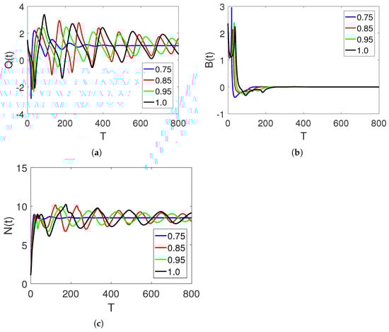
Figure 1.
Curve sketches of classes , , and on different arbitrary fractional orders, 0.85, 0.95, and 1, and time durations on interval .
Figure 2a–d show the dependencies of each market quantity on the agents at different fractional orders. These characteristics reflect a chaotic dynamic system.
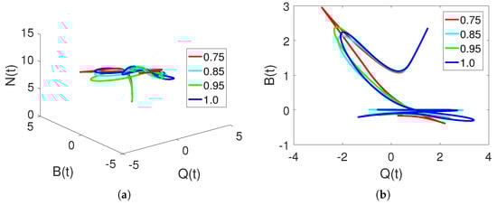
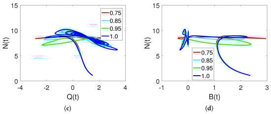
Figure 2.
Chaotic dynamics of , , and classes on different arbitrary orders at fractal dimensions , and 1, and time durations based on changing values of .
In Figure 3a–c, curve sketches of the three stock market financial bubble model compartments based on using the obtained numerical scheme are illustrated. As the shadow price of the net worth increases, the bubbles decrease as the net worth quantity increases. At first, the given market agents fluctuate. However, they stabilize over time. Note that lowering the order may cause a reduction in wavelength.
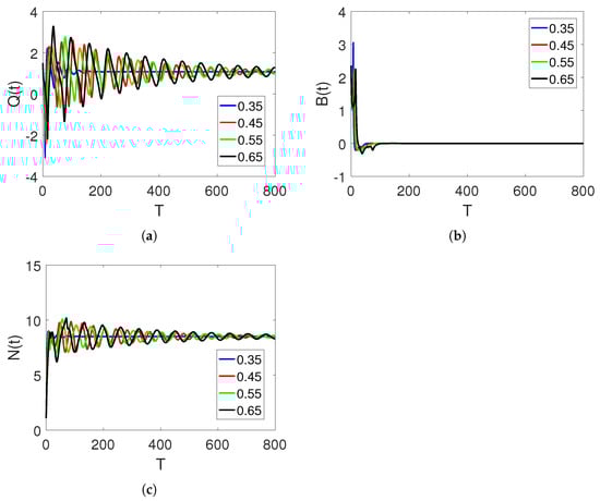
Figure 3.
Curve sketches of classes , , and on different arbitrary fractional orders, 0.45, 0.55, and , and time durations on interval .
Figure 4a–d show the dependencies of market quantity on the agents at smaller fractional orders. These characteristics reflect a chaotic dynamical system.
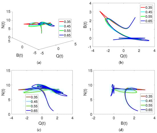
Figure 4.
Chaotic dynamics of , , and classes on different arbitrary orders at fractal dimensions , and , and time durations based on changing values of .
In Figure 5a–c, curve sketches of the three stock market financial bubble model compartments based on using the obtained numerical scheme are illustrated. As the shadow price of the net worth increases, the bubbles decrease as the net worth quantity increases. At first, the given market agents fluctuate. However, they stabilize over time. Note that lowering the order may cause more reductions in wavelength; this time, stability is achieved more quickly.
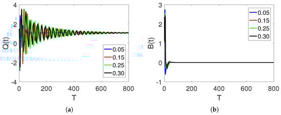
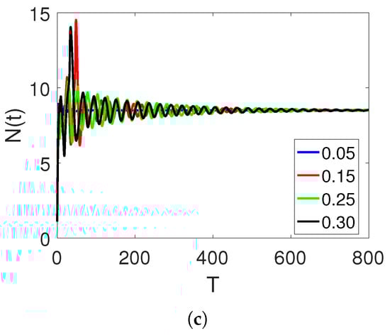
Figure 5.
Curve sketches of classes , , and on different arbitrary fractional orders, 0.15, 0.25, and , and time durations on interval .
Figure 6a–d show the dependencies of each market quantity on the agents at much smaller fractional orders. These characteristics again reflect the chaotic properties of a dynamic system.
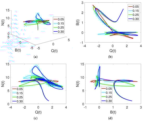
Figure 6.
Chaotic dynamics of , , and classes on different arbitrary orders at fractal dimensions , and , and time durations based on changing values of .
Sensitivity of Parameters
Figure 7a–c present curve sketches of the three stock market financial bubble model compartments based on . Here, the fluctuation is increased, and the wavelength is decreased.
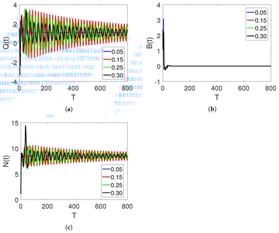
Figure 7.
Curve sketches of classes , , and on different arbitrary fractional orders 0.15, 0.25, and , and time durations on interval , where and .
Figure 8a–c present curve sketches of the three stock market financial bubble model compartments based on in the proposed piecewise model. They are shown to illustrate the sensitivity of the parameters to the same fractional orders as before.
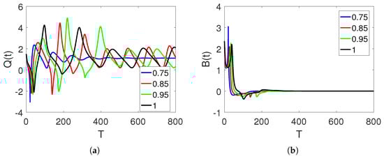
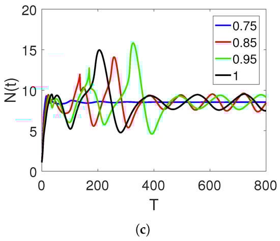
Figure 8.
Curve sketches of , , and classes on different arbitrary fractional orders 0.85, 0.95, and 1, and time durations on interval , where and .
Figure 9a–c present curve sketches of the three stock market financial bubble model compartments based on . Here, the sensitivity is the same as before.
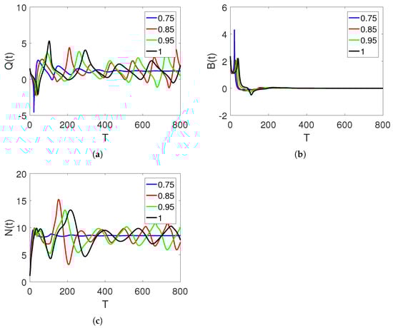
Figure 9.
Curve sketches of classes , , and on different arbitrary fractional orders , 0.85, 0.95, and 1, and time durations on interval , where .
Next, in Figure 10a–c, we provide graphical representations of the three compartments by extending the value of , which regulates the system to achieve stability very quickly.
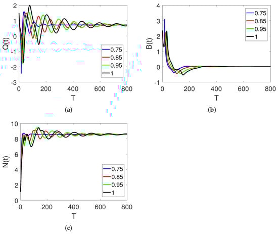
Figure 10.
Curve sketches of classes , , and on different arbitrary fractional orders 0.85, 0.95, and 1, and time durations on interval , where .
6. Summary
This article presents an analysis of a novel framework for studying global derivative financial stock market bubbles, utilizing the Atangana–Baleanu derivative operator. The study successfully establishes the existence and uniqueness of intervals for the considered problem by employing the fixed point theory. A numerical solution method based on the iterative Newton polynomial method is applied to the new model, incorporating a global order with an additional degree of freedom. Numerical simulations of the three compartments are conducted using six variations of data, considering the arbitrary orders of time duration. The impacts of the fractional-order parameters on the global derivative dynamics are also examined. Curve sketches are presented for both the fractional and integer orders, demonstrating a close race to equilibrium. These advancements provide valuable insights for predicting and controlling global phenomena by analyzing the dynamics of different quantities and considering variations in shadow prices, financial bubbles, and stock market net-worth parameters.
Author Contributions
Conceptualization, B.L.; methodology, B.L.; software, B.L.; validation, B.L. and B.Z.; formal analysis, B.L. and B.Z.; data curation, B.L. and K.C.; writing—original draft preparation, B.L., K.C. and B.Z.; writing—review and editing, B.L. and B.Z.; funding acquisition, B.L. All authors have read and agreed to the published version of the manuscript.
Funding
This work has been supported by the Natural Science Foundation of Anhui Province (Grant No. 2008085QA09) and the Science Foundation of the Anhui Education Department (Grant No. KJ2021A0482).
Data Availability Statement
Not applicable.
Conflicts of Interest
The authors declare no conflict of interest.
References
- Shilnikov Pavlovich, L. A case of the existence of a denumerable set of periodic motions. In Doklady Akademii Nauk; Russian Academy of Sciences: Moscow, Russia, 1965; Volume 160, pp. 558–561. [Google Scholar]
- Bella, G.; Mattana, P.; Venturi, B. Shilnikov chaos in the Lucas model of endogenous growth. J. Econ. Theory 2017, 172, 451–477. [Google Scholar] [CrossRef]
- Ben, B.; Gertler, M. VAgency costs. Net Worth Bus. Fluct. Am. Econ. Rev. 1989, 79, 14–31. [Google Scholar]
- Carlstrom, C.T.; Fuerst, T.S. Agency costs, net worth, and business fluctuations: A computable general equilibrium analysis. Am. Econ. Rev. 1997, 87, 893–910. [Google Scholar]
- Nobuhiro, K.; Moore, J. Credit cycles. J. Political Econ. 1997, 105, 211–248. [Google Scholar]
- Bernanke, B.S.; Gertler, M.; Gilchrist, S. The financial accelerator in a quantitative business cycle framework. Handb. Macroecon. 1999, 1, 1341–1393. [Google Scholar]
- He, Q.; Xia, P.; Hu, C.; Li, B. PUBLIC Information, Actual Intervention and Inflation Expectations. Transform. Bus. Econ. 2022, 21, 644–666. [Google Scholar]
- He, Q.; Zhang, X.; Xia, P.; Zhao, C.; Li, S. A Comparison Research on Dynamic Characteristics of Chinese and American Energy Prices. J. Glob. Inf. Manag. (JGIM) 2023, 31, 1–16. [Google Scholar] [CrossRef]
- Giovanni, B.; Mattana, P. Chaos control in presence of financial bubbles. Econ. Lett. 2020, 193, 109314. [Google Scholar]
- Miao, J.; Wang, P. Banking bubbles and financial crises. J. Econ. Theory 2015, 157, 763–792. [Google Scholar] [CrossRef]
- Podlubny, I. Geometric and physical interpretation of fractional integration and fractional differentiation. J. Fract. Calc. Appl. 2002, 5, 367–386. [Google Scholar]
- Miller, K.S.; Ross, B. An Introduction to the Fractional Calculus and Fractional Differential Equations; Wiley: Hoboken, NJ, USA, 1993. [Google Scholar]
- Machado, J.T.; Kiryakova, V.; Mainardi, F. Recent history of fractional calculus. Commun. Nonlinear Sci. Numer. Simul. 2011, 16, 1140–1153. [Google Scholar] [CrossRef]
- Podlubny, I. Fractional Differential Equations: An Introduction to Fractional Derivatives, Fractional Differential Equations, to Methods of Their Solution and Some of Their Applications; Elsevier: Amsterdam, The Netherlands, 1998. [Google Scholar]
- Lakshmikantham, V.; Leela, S.; Devi, J.V. Theory of Fractional Dynamic Systems; CSP: St. Paul, MN, USA, 2009. [Google Scholar]
- Baleanu, D.; Diethelm, K.; Scalas, E.; Trujillo, J.J. Fractional Calculus: Models and Numerical Methods; World Scientific: Singapore, 2012; Volume 3. [Google Scholar]
- Yang, X.-J. Advanced Local Fractional Calculus and Its Applications; World Scientific: Singapore, 2012; Volume 1. [Google Scholar]
- Hilfer, R. (Ed.) Applications of Fractional Calculus in Physics; World Scientific: Singapore, 2000. [Google Scholar]
- Rahman, M.; Althobaiti, A.; Riaz, M.B.; Al-Duais, F.S. A Theoretical and Numerical Study on Fractional Order Biological Models with Caputo Fabrizio Derivative. Fractal Fract. 2022, 6, 446. [Google Scholar] [CrossRef]
- Khan, S.A.; Shah, K.; Zaman, G.; Jarad, F. Existence theory and numerical solutions to smoking model under Caputo-Fabrizio fractional derivative. Chaos Interdiscip. J. Nonlinear Sci. 2019, 29, 013128. [Google Scholar] [CrossRef] [PubMed]
- Baleanu, D.; Jajarmi, A.; Mohammadi, H.; Rezapour, S. A new study on the mathematical modelling of human liver with Caputo–Fabrizio fractional derivative. Chaos Solitons Fractals 2020, 134, 109705. [Google Scholar] [CrossRef]
- Ahmad, S.; Dong, Q.; Rahman, M. Dynamics of a fractional-order COVID-19 model under the nonsingular kernel of Caputo-Fabrizio operator. Math. Model. Numer. Simul. Appl. 2022, 2, 228–243. [Google Scholar] [CrossRef]
- Abdon, A.; Baleanu, D. New fractional derivatives with non-local and non-singular kernel: Theory and application to heat transfer model. Therm. Sci. 2016, 20, 763–769. [Google Scholar]
- Zhang, L.; Rahman, M.; Arfan, M.; Ali, A. Investigation of mathematical model of transmission co-infection TB in HIV community with a non-singular kernel. Results Phys. 2021, 8, 104559. [Google Scholar] [CrossRef]
- ur Rahman, M.; Arfan, M.; Shah, Z.; Alzahrani, E. Evolution of fractional mathematical model for drinking under Atangana-Baleanu Caputo derivatives. Phys. Scr. 2021, 96, 115203. [Google Scholar] [CrossRef]
- Liu, X.; Arfan, M.; Rahman, M.U.; Fatima, B. Analysis of SIQR type mathematical model under Atangana-Baleanu fractional differential operator. Comput. Methods Biomech. Biomed. Eng. 2023, 26, 98–112. [Google Scholar] [CrossRef]
- Ghanbari, B.; Atangana, A. A new application of fractional Atangana–Baleanu derivatives: Designing ABC-fractional masks in image processing. Phys. Stat. Mech. Its Appl. 2020, 542, 123516. [Google Scholar] [CrossRef]
- Dokuyucu, M.A. Analysis of a novel finance chaotic model via ABC fractional derivative. Numer. Methods Partial. Differ. Equ. 2021, 37, 1583–1590. [Google Scholar] [CrossRef]
- Li, B.; Liang, H.; He, Q. Multiple and generic bifurcation analysis of a discrete Hindmarsh-Rose model. Chaos Solitons Fractals 2021, 146, 110856. [Google Scholar] [CrossRef]
- Li, B.; Liang, H.; Shi, L.; He, Q. Complex dynamics of Kopel model with nonsymmetric response between oligopolists. Chaos Solitons Fractals 2022, 156, 111860. [Google Scholar] [CrossRef]
- Li, B.; Zhang, T.; Zhang, C. Investigation of financial bubble mathematical model under fractal-fractional Caputo derivative. Fractals 2023, 31, 2350050. [Google Scholar] [CrossRef]
- Li, B.; Zhang, Y.; Li, X.; Eskandari, Z.; He, Q. Bifurcation analysis and complex dynamics of a Kopel triopoly model. J. Comput. Appl. Math. 2023, 426, 115089. [Google Scholar] [CrossRef]
- Özdemir, N.; Uçar, E. Investigating of an immune system-cancer mathematical model with Mittag-Leffler kernel. AIMS Math. 2020, 5, 1519–1531. [Google Scholar] [CrossRef]
- Uçar, E.; Özdemir, N. A fractional model of cancer-immune system with Caputo and Caputo–Fabrizio derivatives. Eur. Phys. J. Plus 2021, 136, 43. [Google Scholar] [CrossRef] [PubMed]
- Evirgen, F.; Ucar, E.; Özdemir, N.; Altun, E.; Abdeljawad, T. The impact of nonsingular memory on the mathematical model of Hepatitis C virus. Fractals 2023, 31, 2340065. [Google Scholar] [CrossRef]
- Atangana, A.; Araz, S.I. New Numerical Scheme with Newton Polynomial: Theory, Methods, and Applications; Academic Press: Cambridge, MA, USA, 2021. [Google Scholar]
- Toufik, M.; Atangana, A. New numerical approximation of fractional derivative with non-local and non-singular kernel: Application to chaotic models. Eur. Phys. J. Plus 2017, 132, 444. [Google Scholar] [CrossRef]


Disclaimer/Publisher’s Note: The statements, opinions and data contained in all publications are solely those of the individual author(s) and contributor(s) and not of MDPI and/or the editor(s). MDPI and/or the editor(s) disclaim responsibility for any injury to people or property resulting from any ideas, methods, instructions or products referred to in the content. |
© 2023 by the authors. Licensee MDPI, Basel, Switzerland. This article is an open access article distributed under the terms and conditions of the Creative Commons Attribution (CC BY) license (https://creativecommons.org/licenses/by/4.0/).