


Adaptive Control for Finite-Time Cluster Synchronization of Fractional-Order Fully Complex-Valued Dynamical Networks

Abstract
:1. Introduction
2. Preliminaries and Modeling
3. Main Results
3.1. Delay-Dependent Adaptive Control
3.2. Delay-Independent Adaptive Control
4. Numerical Simulations

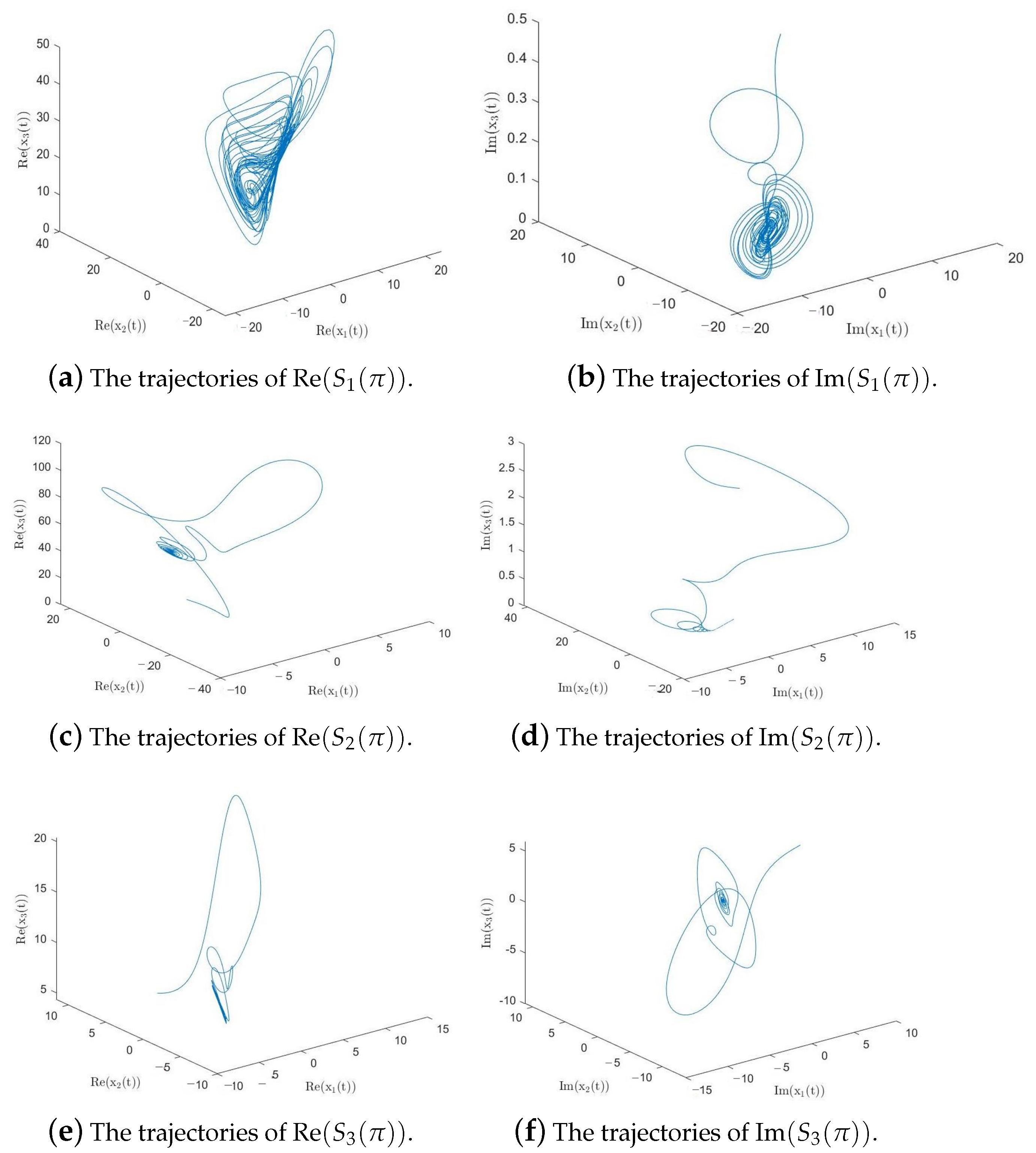
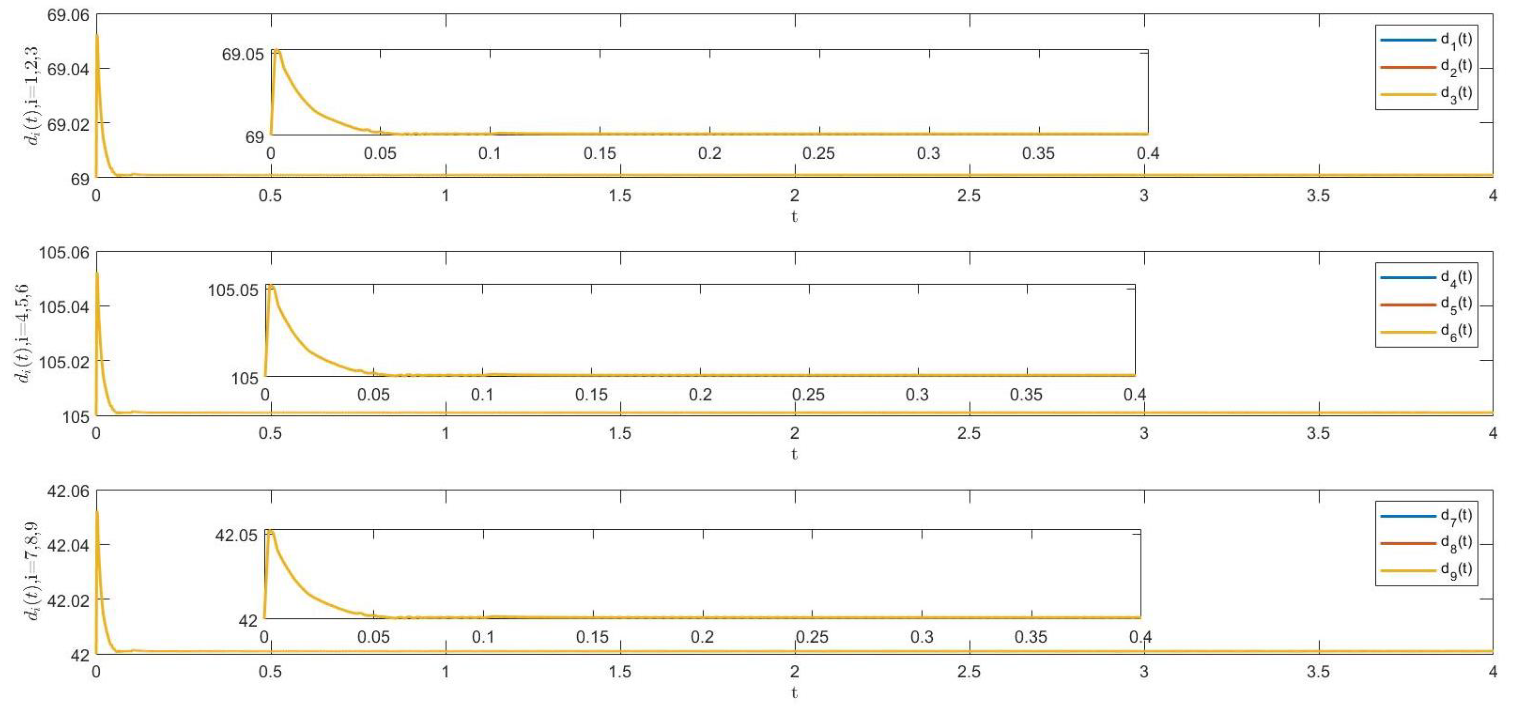
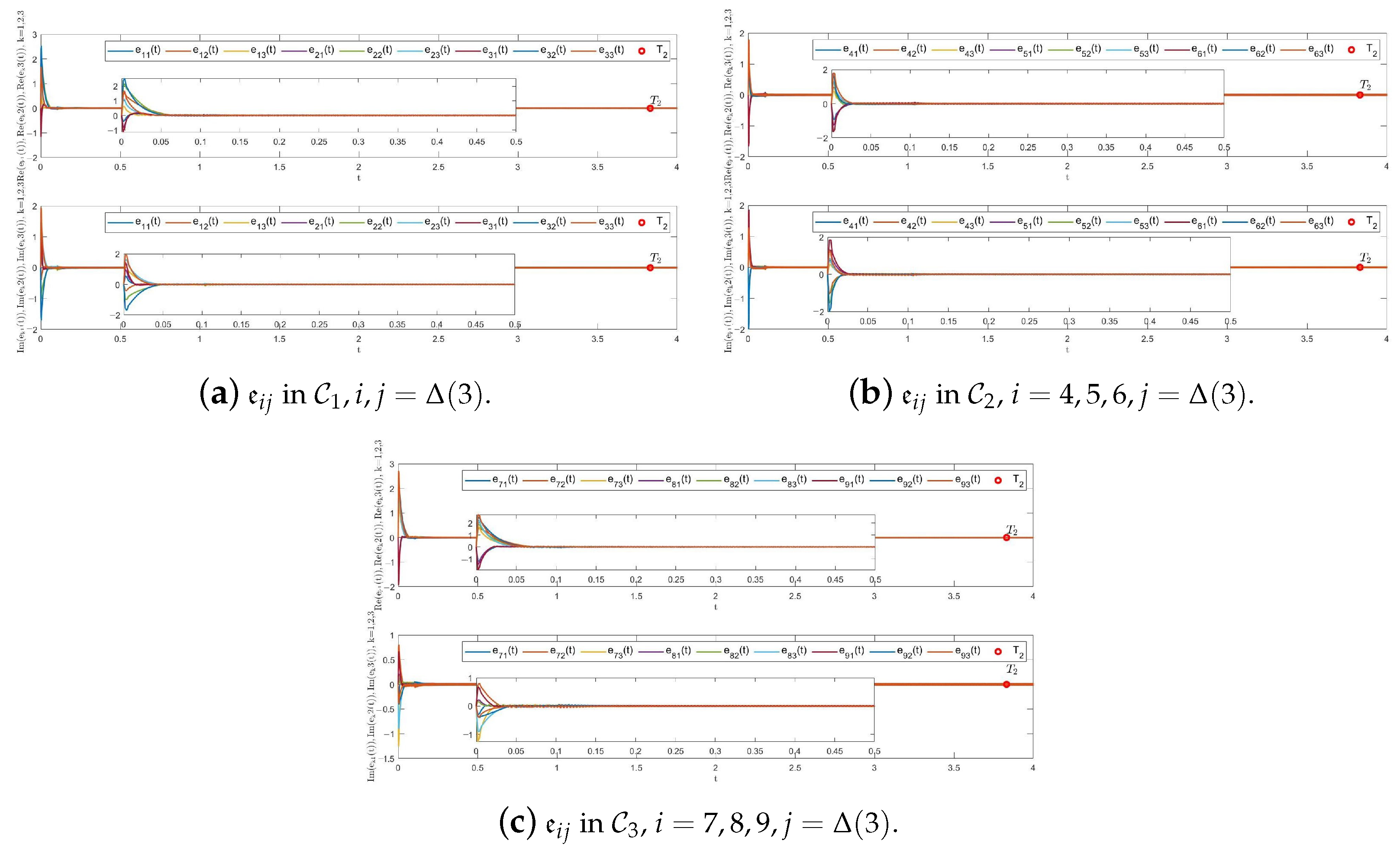
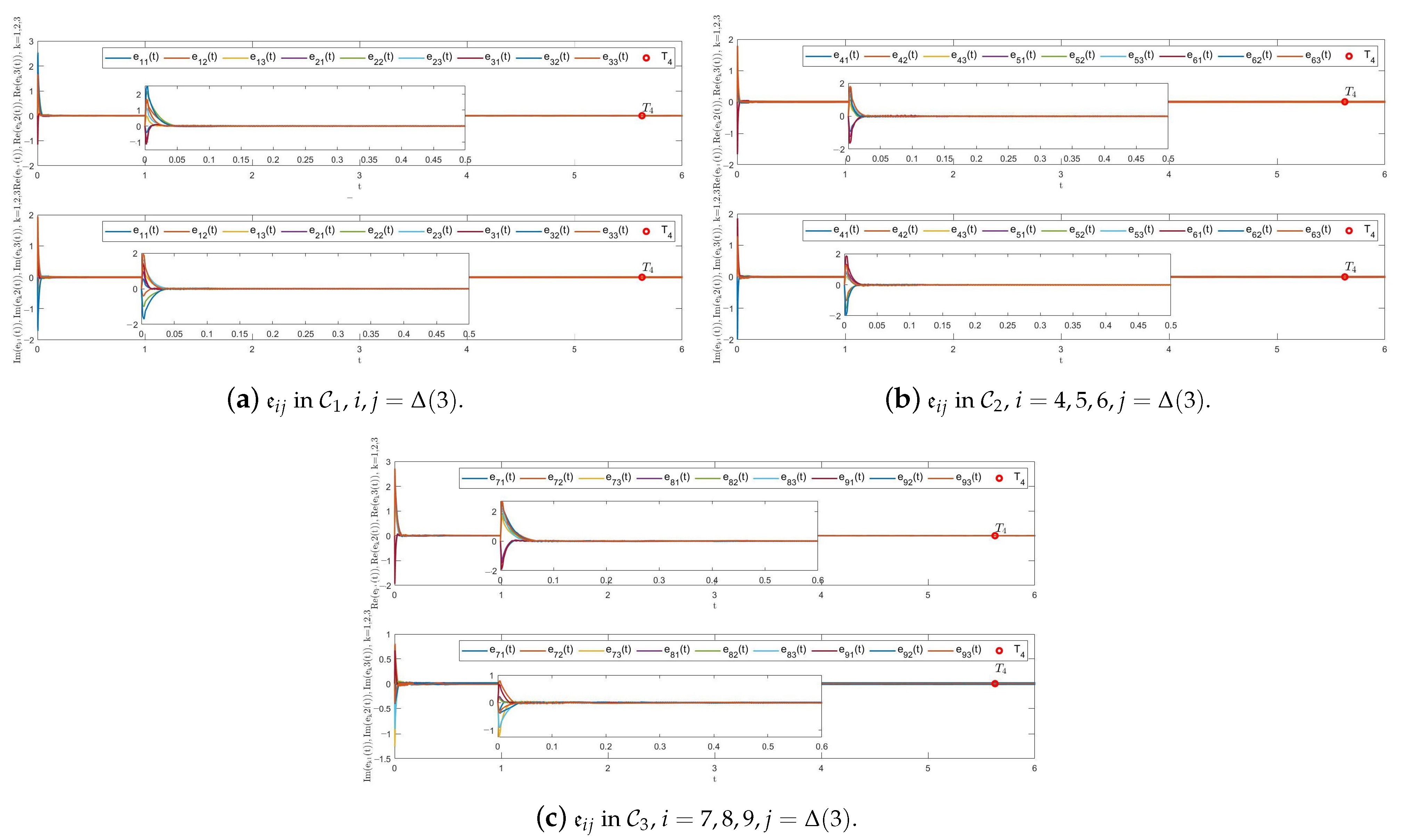
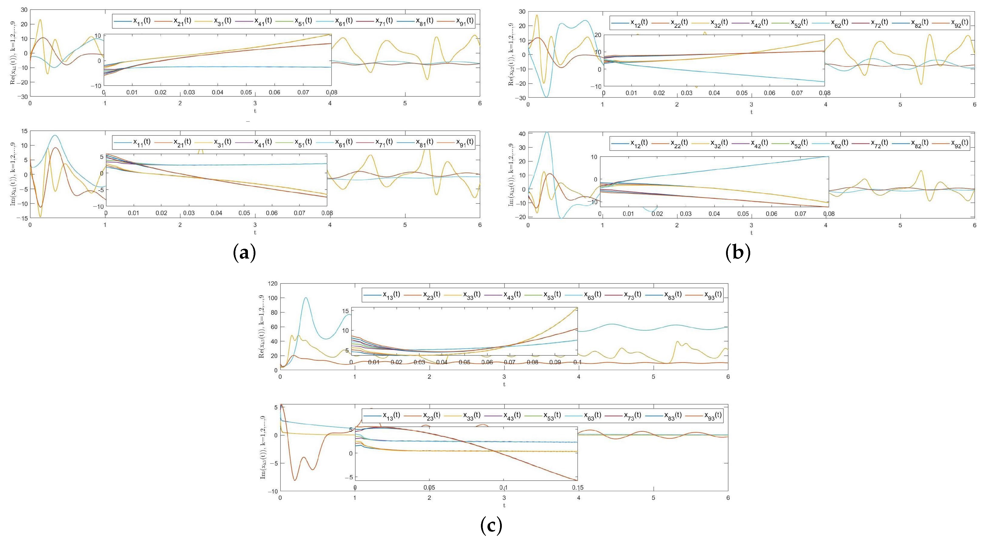
4.1. Example 1
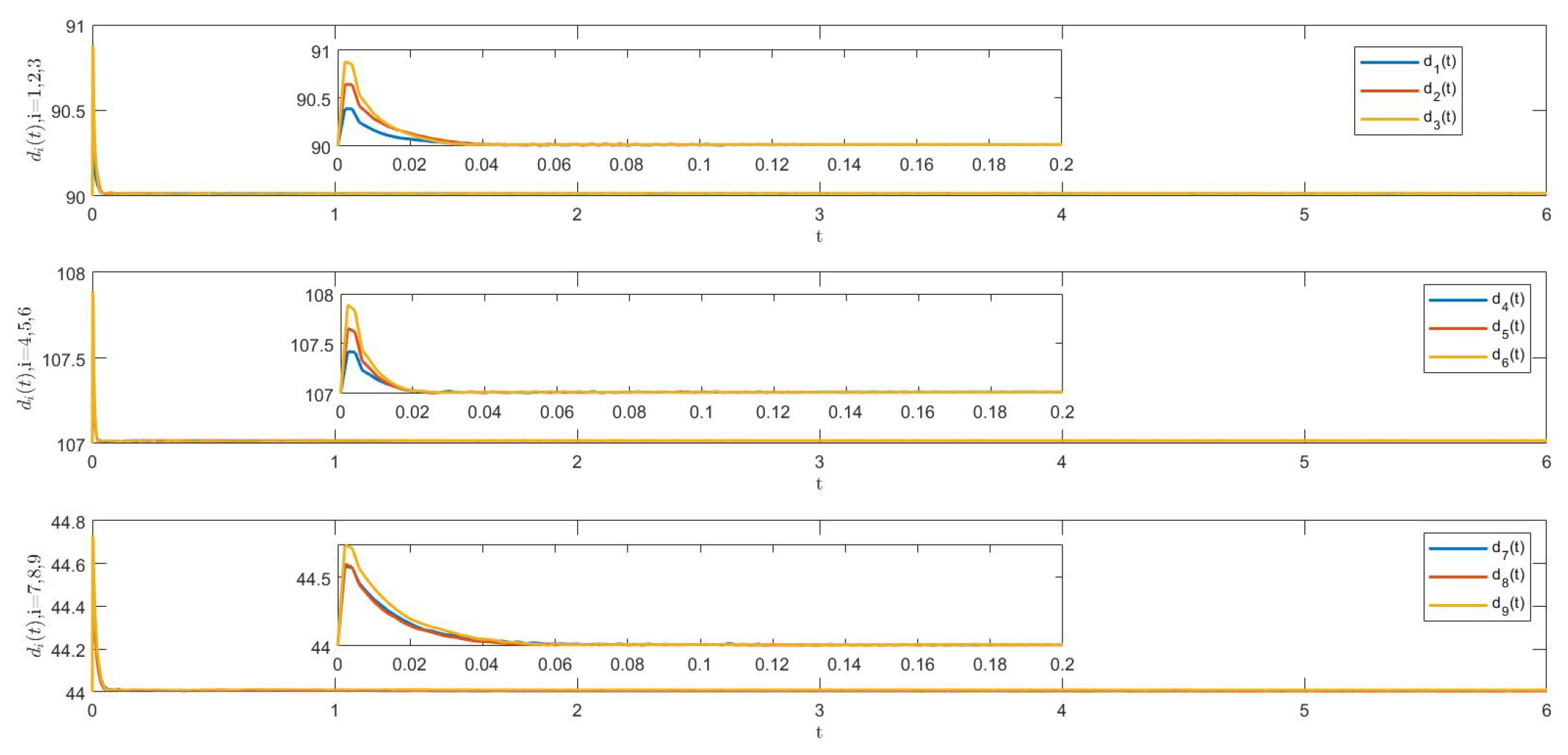
4.2. Example 2
5. Conclusions
Author Contributions
Funding
Institutional Review Board Statement
Informed Consent Statement
Data Availability Statement
Conflicts of Interest
References
- Gan, Q.T.; Xiao, F.; Qin, Y.; Yang, J. Fixed-time cluster synchronization of discontinuous directed community networks via periodically or aperiodically switching control. IEEE Access. 2019, 7, 83306–83318. [Google Scholar] [CrossRef]
- Boonsatit, N.; Rajendran, S.; Lim, C.P.; Jirawattanapanit, A.; Mohandas, P. New Adaptive Finite-Time Cluster Synchronization of Neutral-Type Complex-Valued Coupled Neural Networks with Mixed Time Delays. Fractal Fract. 2022, 6, 515. [Google Scholar] [CrossRef]
- Fan, H.; Shi, K.; Zhao, Y. Pinning impulsive cluster synchronization of uncertain complex dynamical networks with multiple time-varying delays and impulsive effects. Phys. A 2022, 587, 126534. [Google Scholar] [CrossRef]
- He, Q.; Ma, Y. Quantized adaptive pinning control for fixed/preassigned-time cluster synchronization of multi-weighted complex networks with stochastic disturbances. Nonlinear Anal. Hybrid Syst. 2022, 44, 101157. [Google Scholar] [CrossRef]
- Yang, S.; Hu, C.; Yu, J.; Jiang, H.J. Finite-time cluster synchronization in complex-variable networks with fractional-order and nonlinear coupling. Neural Netw. 2021, 135, 212–224. [Google Scholar] [CrossRef]
- Yang, Q.; Wu, H.; Cao, J.D. Pinning exponential cluster synchronization for fractional-order complex dynamical networks with switching topology and mode-dependent impulses. Neurocomputing 2021, 428, 182–194. [Google Scholar] [CrossRef]
- Bhat, S.P.; Bernstein, D.S. Finite-time stability of homogeneous system. In Proceedings of the American Control Conference, Albuquerque, NM, USA, 6 June 1997; pp. 2513–2514. [Google Scholar]
- Cai, S.; Zhou, F.; He, Q. Fixed-time cluster lag synchronization in directed heterogeneous community networks. Phys. A 2019, 525, 128–142. [Google Scholar] [CrossRef]
- Cui, W.; Fang, J.A.; Zhang, W.B.; Wang, X. Finite-time cluster synchronisation of Markovian switching complex networks with stochastic perturbations. IET Control Theory Appl. 2014, 8, 30–41. [Google Scholar] [CrossRef]
- Jiang, S.Q.; Lu, X.B.; Cai, G.L.; Cai, S.M. Adaptive finite-time control for overlapping cluster synchronization in coupled complex networks. Neurocomputing 2017, 266, 188–195. [Google Scholar] [CrossRef]
- Jiang, S.Q.; Lu, X.B.; Cai, G.L.; Cai, S.M. Adaptive fixed-time control for cluster synchronisation of coupled complex networks with uncertain disturbances. Int. J. Syst. Sci. 2017, 48, 3382–3390. [Google Scholar] [CrossRef]
- Liu, X.W.; Chen, T.P. Finite-time and fixed-time cluster synchronization with or without pinning control. IEEE Trans. Cybern. 2018, 48, 240–252. [Google Scholar] [CrossRef]
- Yang, X.S.; Ho, D.W.; Lu, J.Q.; Song, Q. Finite-time cluster synchronization of T-S fuzzy complex networks with discontinuous subsystems and random coupling delays. IEEE Trans. Fuzzy Syst. 2015, 23, 2302–2316. [Google Scholar] [CrossRef]
- Li, H.L.; Cao, J.D.; Jiang, H.J.; Alsaedi, A. Finite-time synchronization and parameter identification of uncertain fractional-order complex networks. Phys. A 2019, 587, 533. [Google Scholar] [CrossRef]
- Li, Y.; Kao, Y.G.; Wang, C.H.; Xia, H.W. Finite-time synchronization of delayed fractional-order heterogeneous complex networks. Neurocomputing 2020, 384, 368–375. [Google Scholar] [CrossRef]
- Peng, X.; Wu, H.Q.; Cao, J.D. Global nonfragile synchronization in finite time for fractional-order discontinuous neural networks with nonlinear growth activations. IEEE Trans. Neural Netw. Learn. Syst. 2019, 30, 2123–2137. [Google Scholar] [CrossRef]
- Xu, Y.; Li, W.X. Finite-time synchronization of fractional-order complex-valued coupled systems. Phys. A 2020, 549, 123903. [Google Scholar] [CrossRef]
- Li, H.L.; Cao, J.D.; Jiang, H.J.; Alsaedi, A. Finite-time synchronization of fractional-order complex networks via hybrid feedback control. Neurocomputing 2018, 320, 69–75. [Google Scholar] [CrossRef]
- Li, H.L.; Cao, J.D.; Jiang, H.J.; Alsaedi, A. Graph theory-based finite-time synchronization of fractional-order complex dynamical networks. J. Frankl. Inst. 2018, 355, 5771–5789. [Google Scholar] [CrossRef]
- Lu, J.Y.; Guo, Y.P.; Ji, Y.D.; Fan, S.S. Finite-time synchronization for different dimensional fractional-order complex dynamical networks. Chaos Solitons Fract. 2020, 130, 109433. [Google Scholar] [CrossRef]
- Jia, Y.; Wu, H.; Cao, J.D. Non-fragile robust finite-time synchronization for fractional-order discontinuous complex networks with multi-weights and uncertain couplings under asynchronous switching. Appl. Math. Comput. 2020, 370, 124929. [Google Scholar] [CrossRef]
- Zhang, L.Z.; Zhong, J.; Lu, J.Q. Intermittent control for finite-time synchronization of fractional-order complex networks. Neural Netw. 2021, 144, 11–22. [Google Scholar] [CrossRef] [PubMed]
- Jian, J.; Wang, P. Lagrange α-exponential stability and α-exponential convergence for fractional-order complex-valued neural networks. Neural Netw. 2017, 91, 1–10. [Google Scholar] [CrossRef]
- Kaslik, E.; Radulescu, I.R. Dynamics of complex-valued fractional-order neural networks. Neural Netw. 2017, 89, 39–49. [Google Scholar] [CrossRef]
- Hou, T.Q.; Yu, J.; Hu, C.; Jiang, H.J. Finite-time synchronization of fractional-order complex-variable dynamic networks. IEEE Trans. Syst. Man Cybern.Syst. 2021, 51, 4297–4307. [Google Scholar] [CrossRef]
- Zheng, B.B.; Hu, C.; Yu, J.; Jiang, H.J. Finite-time synchronization of fully complex-valued neural networks with fractional-order. Neurocomputing 2020, 373, 70–80. [Google Scholar] [CrossRef]
- Long, C.Q.; Zhang, G.D.; Zeng, Z.G.; Hu, J.H. Finite-time stabilization of complex-valued neural networks with proportional delays and inertial terms: A non-separation approach. Neural Netw. 2022, 148, 86–95. [Google Scholar] [CrossRef]
- Das, S.; Das, P.; Das, P. Dynamics and control of multidrug-resistant bacterial infection in hospital with multiple delays. Commun. Nonlinear Sci. Numer. Simul. 2020, 89, 105279. [Google Scholar] [CrossRef]
- Ren, Y.; Jiang, H.J.; Li, J.R.; Lu, B.L. Finite-time synchronization of stochastic complex networks with random coupling delay via quantized aperiodically intermittent control. Neurocomputing 2021, 420, 337–348. [Google Scholar] [CrossRef]
- Xiong, K.L.; Yu, J.; Hu, C.; Jiang, H.J. Synchronization in finite/fixed time of fully complex-valued dynamical networks via nonseparation approach. J. Frankl. Inst. 2020, 357, 473–493. [Google Scholar] [CrossRef]
- Kilbas, A.A.; Srivastava, H.M.; Trujillo, J.J. Theory and Applications of Fractional Differential Equations; Elsevier: New York, NY, USA, 2006. [Google Scholar]
- Podlubny, I. Fractional Differential Equations; Academic Press: New York, NY, USA, 1999. [Google Scholar]
- Kang, Q.; Yang, Q.; Yang, J.; Gan, Q.; Li, R. Synchronization in finite-time of delayed fractional-order fully complex-valued dynamical networks via non-separation method. Entropy 2022, 24, 1460. [Google Scholar] [CrossRef]
- Xia, W.G.; Cao, J.D. Pinning synchronization of delayed dynamical networks via periodically intermittent control. Chaos 2009, 19, 013120. [Google Scholar] [CrossRef] [PubMed]
- Cai, S.M.; He, Q.B.; Hao, J.J.; Liu, Z.R. Exponential synchronization of complex networks with nonidentical time-delayed dynamical nodes. Phys. A 2010, 374, 2539–2550. [Google Scholar] [CrossRef]
- Yu, J.; Hu, C.; Jiang, H.J. Corrogendum to “Projective synchronization for fractional neural networks”. Neural Netw. 2015, 67, 152–154. [Google Scholar] [CrossRef]
- Xu, Q.; Zhuang, S.X.; Liu, S.J.; Xiao, J. Decentralized adaptive coupling synchronization of fractional-order complex-variable dynamical networks. Neurocomputing 2016, 186, 119–126. [Google Scholar] [CrossRef]
- Danca, M. Controlling chaos in discontinuous dynamical systems. Chaos Solitons Fract. 2014, 22, 605–612. [Google Scholar] [CrossRef]
- Forti, M.; Grazzini, M.; Nistri, P.; Pancioni, L. Generalized Lyapunov approach for convergence of neural networks with discontinuous or non-Lipschitz activations. Phys. D 2006, 214, 88–99. [Google Scholar] [CrossRef]

Disclaimer/Publisher’s Note: The statements, opinions and data contained in all publications are solely those of the individual author(s) and contributor(s) and not of MDPI and/or the editor(s). MDPI and/or the editor(s) disclaim responsibility for any injury to people or property resulting from any ideas, methods, instructions or products referred to in the content. |
© 2023 by the authors. Licensee MDPI, Basel, Switzerland. This article is an open access article distributed under the terms and conditions of the Creative Commons Attribution (CC BY) license (https://creativecommons.org/licenses/by/4.0/).
Share and Cite
Xiang, K.; Kang, Q.; Chang, H.; Yang, J. Adaptive Control for Finite-Time Cluster Synchronization of Fractional-Order Fully Complex-Valued Dynamical Networks. Fractal Fract. 2023, 7, 645. https://doi.org/10.3390/fractalfract7090645
Xiang K, Kang Q, Chang H, Yang J. Adaptive Control for Finite-Time Cluster Synchronization of Fractional-Order Fully Complex-Valued Dynamical Networks. Fractal and Fractional. 2023; 7(9):645. https://doi.org/10.3390/fractalfract7090645
Chicago/Turabian StyleXiang, Kaiquan, Qiaokun Kang, Hao Chang, and Jing Yang. 2023. "Adaptive Control for Finite-Time Cluster Synchronization of Fractional-Order Fully Complex-Valued Dynamical Networks" Fractal and Fractional 7, no. 9: 645. https://doi.org/10.3390/fractalfract7090645
APA StyleXiang, K., Kang, Q., Chang, H., & Yang, J. (2023). Adaptive Control for Finite-Time Cluster Synchronization of Fractional-Order Fully Complex-Valued Dynamical Networks. Fractal and Fractional, 7(9), 645. https://doi.org/10.3390/fractalfract7090645