An Accurate Approach to Simulate the Fractional Delay Differential Equations

Abstract

The fractional Legendre polynomials (FLPs) that we present as an effective method for solving fractional delay differential equations (FDDEs) are used in this work. The Liouville–Caputo sense is used to characterize fractional derivatives. This method uses the spectral collocation technique based on FLPs. The proposed method converts FDDEs into a set of algebraic equations. We lay out a study of the convergence analysis and figure out the upper bound on error for the approximate solution. Examples are provided to demonstrate the precision of the suggested approach.

1. Introduction

In the hope of simulating a variety of physical events, it is crucial to use differential equations based on fractional-order operators [1,2]. Some applications of these equations include earthquake simulation, damping principles, fluid dynamics, biology, physics, and engineering [3,4,5,6,7]. Numerous techniques have been employed to locate appropriate solutions to these equations depending on their physical structure. The majority of the current systems are flawed and unworkable considering the actual physical existence of these problems. The numerical findings show the full reliability of the proposed algorithms [8,9,10]. Since explicit exact solutions for FDEs are still lacking, approximation and numerical techniques such as the spectral collocation method (SCM), FEM, FVM, and many others have been used to solve many fractional models [11,12,13,14,15]. The paper’s primary goal is to use the mentioned algorithm ([16,17]) to obtain the numerical solution of the following FDDE using SCM depending on the fractional Legendre polynomials [18]:

$$D^{\alpha }u\left(x\right)=f\left(x,u\left(x\right),u\left(g\right(x\left)\right)\right),0<x<1,0<\alpha \le 2,$$

(1)

where

$$u\left(0\right)={\lambda }_0,u\left(1\right)={\lambda }_1,$$

(2)

where the order of the Liouville–Caputo fractional is $\alpha$. The delay function is a function g that satisfies condition $a\le g\left(x\right)\le x,x\in [a,b]$ and $g\left(x\right)\in C[a,b]$. Also, we shall calculate an upper bound for the estimated solution’s resulting error and the convergence will be studied. In ([19,20]), the authors used spline functions to study both the error and stability analysis for first-order delay differential equations. We plan to discretize Equation (1) using the Legendre collocation method to produce an algebraic system of equations (linear/nonlinear) and solve it.

The manuscript is structured as follows: Section 2 presents the definitions and approximate formula for the fractional derivative. Section 3 provides some thoughts on the recently revealed fractional-order Legendre polynomials. The polynomials approximation and error estimation are discussed in Section 4. The implementation of the Legendre spectral method for solving FDDE is introduced in Section 5. Section 6 also discusses numerical simulation. We provide the conclusions and some observations in Section 7.

2. Preliminaries and Notations

Definition 1.

The following formula defines the fractional derivative of order α of Liouville–Caputo ([15,21]):

$$D^{\alpha }f\left(t\right)=\left\{\begin{array}{cc}\frac{1}{\Gamma (m-\alpha )}{\int }_0^t\frac{f^{\left(m\right)}\left(\xi \right)}{{(t-\xi )}^{\alpha -m+1}}d\xi ,\hfill & m-1<\alpha <m,\hfill \\ f^{\left(m\right)}\left(t\right),\hfill & \alpha =m\in \mathbb{N},\hfill \end{array}\right.$$

where

$$D^{\alpha }{t}^n=\left\{\begin{array}{cc}0,\hfill & \mathrm{for}n\in {\mathbb{N}}_0\mathrm{and}n<\lceil \alpha \rceil ;\hfill \\ \frac{\Gamma (n+1)}{\Gamma (n+1-\alpha )}{t}^{n-\alpha },\hfill & \mathrm{for}n\in {\mathbb{N}}_0\mathrm{and}n\ge \lceil \alpha \rceil .\hfill \end{array}\right.$$

(3)

Additionally, a generalization of Taylor’s formula is introduced based on the fractional derivative of Liouville–Caputo [22]. Assume that

$$D^{k\alpha }f\left(t\right)\in C(0,a],\mathrm{for}k=0,1,...,n+1,\mathrm{where}0<\alpha \le 1,$$

then,

$$f\left(t\right)=\sum _{i=0}^n\frac{x^{i\alpha }}{\Gamma (i\alpha +1)}{D}^{i\alpha }f\left(0^{+}\right)+\frac{\left(D^{(n+1)\alpha }f\right)\left(\xi \right)}{\Gamma \left(\right(n+1)\alpha +1)}{t}^{(n+1)\alpha },0\le \xi \le t,\forall t\in (0,a].$$

(4)

3. Legendre Polynomials of Fractional Order

Since the well-known Legendre polynomials $L_k\left(z\right)$ are defined on $[-1,1]$ ([23,24]), we introduce the shifted Legendre polynomials $L_k^{*}\left(t\right)$ by inserting $z=2t-1$ to use these polynomials on $[0,1]$.

We shall introduce the fractional-order Legendre polynomials in this section. By changing the variables $t=x^{\nu }$ and $\nu >0$ on $L_k^{*}\left(t\right)$, these polynomials will be obtained. We represent FLPs, $L_k^{*}\left(x^{\nu }\right)$ by $P_k^{\nu }\left(x\right)$. We note that the recurrence formula for $P_k^{\nu }\left(x\right)$ may be deduced from the recurrence relation of $L_k^{*}\left(t\right)$ [18]:

$$P_{k+1}^{\nu }\left(x\right)=\frac{(2k+1)(2x^{\nu }-1)}{(k+1)}{P}_k^{\nu }\left(x\right)-\frac{k}{k+1}{P}_{k-1}^{\nu }\left(x\right),P_0^{\nu }\left(x\right)=1,P_1^{\nu }\left(x\right)=2x^{\nu }-1,k=1,2,\dots ,.$$

The analytic form of the FLPs, $P_k^{\nu }\left(x\right)$ of degree $\nu k$ is given by:

$$P_k^{\nu }\left(x\right)=\sum _{i=0}^k{(-1)}^{k+i}\frac{(k+i)!}{(k-i)!{(i!)}^2}{x}^{i\nu }.$$

(5)

Note that $P_k^{\nu }\left(0\right)={(-1)}^k$ and $P_k^{\nu }\left(1\right)=1$.

Lemma 1

([25]). According to the weight function $w^{\nu }\left(x\right)=x^{\nu -1}$, the fractional-order polynomials $P_i^{\nu }\left(x\right)$ are orthogonal over $[0,q]$. Therefore, we obtain

$${\int }_0^1{P}_i^{\nu }\left(x\right)P_j^{\nu }\left(x\right)w^{\nu }\left(x\right)dx=\frac{{\delta }_{ij}}{\nu (2i+1)}.$$

Proof. 

The formula can be obtained directly by taking $t=x^{\nu }$, in the orthogonality condition ${\int }_0^1{L}_i^{*}\left(t\right)L_j^{*}\left(t\right)dt=\frac{{\delta }_{ij}}{2i+1}.$ □

4. Approximating Polynomials and Estimating Errors

Let a non-negative, integrable, real-valued function spanning the range $(0,1)$ be denoted by $w^{\nu }\left(x\right)=x^{\nu -1},\nu >0$. In the first $(m+1)$-terms of FLPs, the function $u\left(x\right)\in L_{w^{\nu }}^2$, which is a square-integrable function in $[0,1]$, can be represented and approximated as follows:

$$u_m^{\nu }\left(x\right)=\sum _{i=0}^m{c}_i{P}_i^{\nu }\left(x\right).$$

(6)

The error estimate for this approximation in $w^{\nu }$-norm is provided by the following theorem.

Theorem 1.

The error bound can be calculated using the following formula if $u_m^{\nu }$ is the best estimation to $u\left(x\right)$ out of $V_m^{\nu }:=\mathit{span}\{P_0^{\nu }\left(x\right),P_1^{\nu }\left(x\right),\dots ,P_m^{\nu }\left(x\right)\},$ and $D^{i\nu }u\left(x\right)\in C(0,1]$ for $i=0,1,\dots ,m+1$:

$$\parallel u-u_m^{\nu }{\parallel }_{w^{\nu }}\le \frac{e^{(m+1)\nu -\frac{\theta }{12(m+1)\nu }}}{{\left((m+1)\nu \right)}^{(m+1)\nu +\frac{1}{2}}}\frac{{\gamma }_{\nu }}{\sqrt{2\pi (2m+3)\nu }},$$

where  $0<\theta <1$, ${\gamma }_{\nu }={sup}_{x\in (0,1]}|D^{(m+1)\nu }u\left(x\right)|.$

Proof. 

As an approximate representation of $u\left(x\right)$ and denoted by $y\left(x\right)$, consider the generalized Taylor’s polynomial as follows:

$$y\left(x\right)=\sum _{i=0}^m\frac{x^{i\nu }}{\Gamma (i\nu +1)}{D}^{i\nu }u\left(0^{+}\right),x\in (0,1],$$

where it is known that the following error bound exists and:

$$|u\left(x\right)-y\left(x\right)|=\left|\frac{x^{(m+1)\nu }}{\Gamma \left(\right(m+1)\nu +1)}{D}^{(m+1)\nu }u\left({\xi }_x\right)\right|\le {\gamma }_{\nu }\frac{x^{(m+1)\nu }}{\Gamma \left(\right(m+1)\nu +1)}=\frac{{\gamma }_{\nu }{x}^{(m+1)\nu }}{\left(\right(m+1\left)\nu \right)!}.$$

Since $u_m^{\nu },y\left(x\right)\in V_m^{\nu }$ and $u_m^{\nu }$ is the best approximation to $u\left(x\right)$ out of $V_m^{\nu }$, then

$$\begin{array}{cc}\hfill \parallel u-u_m^{\nu }{\parallel }_{w^{\nu }}^2& \le {\parallel u-y\parallel }_{w^{\nu }}^2\le {\left(\frac{{\gamma }_{\nu }}{\left(\right(m+1\left)\nu \right)!}\right)}^2{\int }_0^1{x}^{\nu -1}{x}^{2(m+1)\nu }dx\hfill \\ & ={\left(\frac{{\gamma }_{\nu }}{\left(\right(m+1\left)\nu \right)!}\right)}^2\frac{1}{(2m+3)\nu },\hfill \end{array}$$

this together with the well-known Stirling formula ($n!=\sqrt{2\pi }{n}^{n+1/2}{e}^{-n+\theta /12n}$, for some $(0<\theta <1)$ lead to the desired result. □

The primary formula for calculating an approximation of the Liouville–Caputo fractional derivative is given in the following theorem.

Theorem 2.

Let $u\left(x\right)$ be as described in (6) and $\alpha >0,$ then:

$$D^{\alpha }\left(u_m^{\nu }\left(x\right)\right)=\sum _{i=\lceil \alpha \rceil }^m\sum _{k=\lceil \alpha \rceil }^i{c}_i{w}_{i,k}^{(\nu ,\alpha )}{x}^{\nu k-\alpha },w_{i,k}^{(\nu ,\alpha )}=\frac{{(-1)}^{(i+k)}(i+k)!\Gamma (\nu k+1)}{(i-k)!{(\left(k\right)!)}^2\Gamma (\nu k-\alpha +1)}.$$

(7)

Proof. 

We can obtain this formula directly by using the linearity properties of the Liouville–Caputo operation and then employing Equation (3) in Formula (5) with some simplification. □

Theorem 3.

The error $|E_T\left(m\right)|=|D^{\alpha }u\left(x\right)-D^{\alpha }{u}_m^{\nu }\left(x\right)|$ in approximating $D^{\alpha }u\left(x\right)$ by $D^{\alpha }{u}_m^{\nu }\left(x\right)$ is bounded by:

$$|E_T\left(m\right)|\le |\sum _{i=m+1}^{\infty }{c}_i\left(\sum _{k=\lceil \alpha \rceil }^i\sum _{j=0}^{k-\lceil \alpha \rceil }{\Theta }_{i,j,k}\right)|,$$

(8)

where

$${\Theta }_{i,j,k}=\frac{{(-1)}^{i+k}(i+k)!(2j+1)}{(i-k)!{(\left(k\right)!)}^2\Gamma (\nu k-\alpha +1)}\times \sum _{r=0}^j\frac{{(-1)}^{j+r}(j+r)!}{(j-r)!{(r!)}^2(\nu k-\alpha +r+1)},j=0,1,\dots .$$

Proof. 

The proof can be found in [24]. □

5. Implementation of Legendre-SCM for Solving FDDE

Consider the FDDE (1), we first write $u(x$) as:

$$u_m^{\nu }\left(x\right)=\sum _{i=0}^m{c}_i{P}_i^{\nu }\left(x\right).$$

(9)

From Equations (1) and (9) and Theorem 2, we have:

$$\sum _{i=\lceil \alpha \rceil }^m\sum _{k=\lceil \alpha \rceil }^i{c}_i{w}_{i,k}^{(\nu ,\alpha )}{x}^{\nu k-\alpha }=f\left(x,\sum _{i=0}^m{c}_i{P}_i^{\nu }\left(x\right),\sum _{i=0}^m{c}_i{P}_i^{\nu }\left(g\left(x\right)\right)\right).$$

(10)

We now collocate Equation (10) at $(m+1-\lceil \alpha \rceil )$ points $x_p$, $p=0,1,\dots ,m-\lceil \alpha \rceil$ as:

$$\sum _{i=\lceil \alpha \rceil }^m\sum _{k=\lceil \alpha \rceil }^i{c}_i{w}_{i,k}^{(\nu ,\alpha )}{x}_p^{\nu k-\alpha }=f\left(x_p,\sum _{i=0}^m{c}_i{P}_i^{\nu }\left(x_p\right),\sum _{i=0}^m{c}_i{P}_i^{\nu }\left(g\left(x_p\right)\right)\right).$$

(11)

We utilize the roots of the fractional Legendre polynomial $P_{m+1-\lceil \alpha \rceil }^{\nu }\left(x\right)$ for suitable collocation nodes.

From (9) in (2), and use the properties of the Formula (5), we can obtain the following equations:

$$\sum _{i=0}^m{(-1)}^i{c}_i={\lambda }_0,\sum _{i=0}^m{c}_i={\lambda }_1.$$

(12)

Using Equation (11) and $\lceil \alpha \rceil$ equations of B.Cs gives $(m+1)$ algebraic equations in the unknown $c_i,i=0,1,\dots ,m$, which can be solved. Consequently, $u\left(x\right)$ for (1) can be found.

6. Numerical Results

Example 1.

Consider the following differential equation for a linear fractional delay:

$$D^{0.5}u\left(x\right)+u(x/4)+2\sqrt{x}u\left(x\right)=2x+0.5(\sqrt{x}+\sqrt{\mathrm{\pi }}),$$

(13)

with the initial condition:

$$u\left(0\right)=0.$$

(14)

Using the provided method and $m=2$, we arrive at the following approximation of the solution:

$$u_2^{\nu }\left(x\right)=\sum _{n=0}^2{c}_n{P}_n^{\nu }\left(x\right).$$

(15)

Using Equation (11) with $\alpha =0.5$, we have:

$$\begin{array}{c}\hfill \sum _{n=\lceil \alpha \rceil }^2\sum _{k=\lceil \alpha \rceil }^n{c}_n{w}_{n,k}^{(\nu ,\alpha )}{x}_p^{\nu k-\alpha }+\sum _{n=0}^2{c}_n{P}_n^{\nu }(x_p/4)+2\sqrt{x_p}\sum _{n=0}^2{c}_n{P}_n^{\nu }\left(x_p\right)=2x_p+0.5(\sqrt{x_p}+\sqrt{\mathrm{\pi }}),\end{array}$$

(16)

with $p=0,1$ where $x_p$ are roots of $P_2^{\nu }\left(x\right)$ and $x_0=0.0446582,x_1=0.622008,$ at $\nu =0.5$. Using Equations (14) and (15) we get:

$$c_0-c_1+c_2=0.$$

(17)

Now, solving Equations (16) and (17), we get:

$$c_0=1/2,c_1=1/2,c_2=0.0.$$

Thus, using Equation (15) we can get:

$$u\left(x\right)\simeq \frac{1}{2}{P}_0^{\nu }\left(x\right)+\frac{1}{2}{P}_1^{\nu }\left(x\right)+0.0P_2^{\nu }\left(x\right)=\sqrt{x}=\mathit{The}\mathit{exact}\mathit{solution}.$$

Example 2.

Consider the following differential equation for a linear fractional delay:

$$D^{\alpha }u\left(x\right)+e^{-\sqrt{x}/4}u(x/16)-\frac{1}{2\sqrt{x}}u\left(x\right)=1,0<\alpha \le 1,$$

(18)

with

$$u\left(0\right)=1.$$

(19)

The exact solution of Equation (18) at $\alpha =1$ is $u\left(x\right)=e^{\sqrt{x}}$. Using the provided method and $m=4$, we arrive at the following approximation of the solution:

$$u_4^{\nu }\left(x\right)=\sum _{n=0}^4{c}_n{P}_n^{\nu }\left(x\right).$$

(20)

Using Equation (11), we have:

$$\begin{array}{c}\hfill \sum _{n=\lceil \alpha \rceil }^4\sum _{k=\lceil \alpha \rceil }^n{c}_n{w}_{n,k}^{(\nu ,\alpha )}{x}_p^{\nu k-\alpha }+e^{-\sqrt{x_p}/4}\sum _{n=0}^4{c}_n{P}_n^{\nu }(x_p/16)-\frac{1}{2\sqrt{x_p}}\sum _{n=0}^4{c}_n{P}_n^{\nu }\left(x_p\right)=1,\end{array}$$

(21)

with $p=0,1,2,3$ where $x_p$ are roots of $P_4^{\nu }\left(x\right)$ and $x_0=0.004821,x_1=0.108961,$$x_2=0.448887,$ $x_3=0.865957$, at $\nu =0.5$.

Using Equations (19) and (20), we obtain:

$$c_0-c_1+c_2-c_3+c_4=1.$$

(22)

Now, solving Equations (21) and (22), we can obtain:

$$c_0=1.718288,c_1=0.845162,c_2=0.139858,c_3=0.013982,c_4=0.000998.$$

Thus, using Equation (20) we can obtain the approximate solution $u\left(x\right)$ of Example 2.

The approximate solution and the exact one are given in Figure 1 at $\alpha =1$ and $\nu =0.5$. But, the approximate solution with $\alpha (=0.75,0.85)$ is given in Figure 2. These graphs demonstrate that the exact solution and numerical solution are in very good agreement, and the approximate solution exhibits the same behavior.

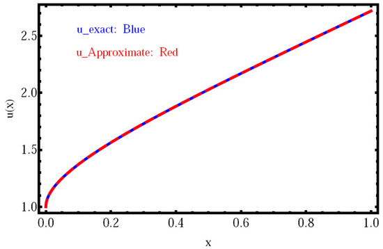
Figure 1. The numerical solution and the exact solution of Example 2.

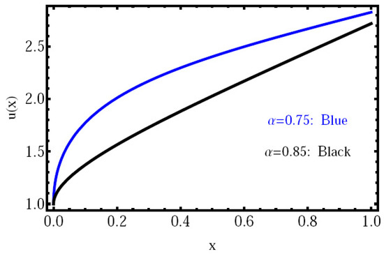
Figure 2. The approximate solution with different values of $\alpha$ of Example 2.

Example 3.

Consider the following non-linear fractional delay differential equation:

$$D^{1.5}u\left(x\right)=u(x-0.5)+u^3\left(x\right)+h\left(x\right),$$

(23)

where $h\left(x\right)=\frac{\Gamma (2\nu +1)}{\Gamma (2\nu -0.5)}{x}^{2\nu -1.5}-{(x-0.5)}^{2\nu }-x^{6\nu }$, with

$$u\left(0\right)=0,u\left(1\right)=1.$$

(24)

Using the provided method and $m=3$, we arrive at the following approximation of the solution:

$$u_m^{\nu }\left(x\right)=\sum _{n=0}^m{c}_n{P}_n^{\nu }\left(x\right).$$

(25)

Using Equation (11), we have:

$$\begin{array}{c}\hfill \sum _{i=\lceil \alpha \rceil }^3\sum _{k=\lceil \alpha \rceil }^i{c}_i{w}_{i,k}^{(\nu ,\alpha )}{x}_p^{\nu k-\alpha }=\sum _{n=0}^3{c}_n{P}_n^{\nu }(x_p-0.5)+{\left(\sum _{n=0}^3{c}_n{P}_n^{\nu }\left(x_p\right)\right)}^3+h\left(x_p\right),\end{array}$$

(26)

with $p=0,1,2$ where $x_p$ are roots of $P_3^{\nu }\left(x\right)$. Using Equations (24) and (25), we obtain:

$$c_0-c_1+c_2-c_3=0,$$

(27)

$$c_0+c_1+c_2+c_3=1.$$

(28)

Solving (26)–(28), we obtain:

$$c_0=1/3,c_1=1/2,c_2=1/6,c_3=0.0.$$

Thus, using Equation (25) at $\nu =1.25$, we can obtain:

$$u\left(x\right)=\frac{1}{3}{P}_0^{\nu }\left(x\right)+\frac{1}{2}{P}_1^{\nu }\left(x\right)+\frac{1}{6}{P}_2^{\nu }\left(x\right)+0.0P_3^{\nu }\left(x\right)=x^{2.5}=x^{2\nu }=\mathit{The}\mathit{exact}\mathit{solution}.$$

Example 4 ((Ikeda system-One delay)).

Consider the Ikeda delay system with one delay, which is described in ([26,27]):

$$D^{\alpha }u\left(t\right)=-\kappa u\left(t\right)+\lambda sin\left(\mu u(t-\tau )\right),1<\alpha \le 2,$$

(29)

where $\kappa ,\lambda ,\mu$, and τ are constants; with

$$u\left(0\right)=u_0,u\left(1\right)=u_1.$$

(30)

Using the provided method and $m=10$, we arrive at the approximation of the solution as in Equation (25). Using Equation (11), we have

$$\begin{array}{c}\hfill \sum _{n=\lceil \alpha \rceil }^m\sum _{k=\lceil \alpha \rceil }^n{c}_n{w}_{n,k}^{(\nu ,\alpha )}{t}_p^{\nu k-\alpha }=-\kappa \sum _{n=0}^m{c}_n{P}_n^{\nu }\left(t_p\right)+\lambda sin\left(\mu \sum _{n=0}^m{c}_n{P}_n^{\nu }(t_p-\tau )\right),\end{array}$$

(31)

with $p=0\left(1\right)8$ where $t_p$ are roots of $P_9^{\nu }\left(t\right)$. Using Equations (25) and (30), we can obtain:

$$\sum _{n=0}^m{(-1)}^n{c}_n=u_0,\sum _{n=0}^m{c}_n=u_1.$$

(32)

Now, solving the system of Equations (31)–(32), we obtain the approximate solution of this model (29).

To conclude this numerical analysis with the simulation; we define the residual error function (REF) as:

$$\mathit{REF}(t,m)=\sum _{n=\lceil \alpha \rceil }^m\sum _{k=\lceil \alpha \rceil }^n{c}_n{w}_{n,k}^{(\nu ,\alpha )}{t}^{\nu k-\alpha }+\kappa \sum _{n=0}^m{c}_n{P}_n^{\nu }\left(t\right)-\lambda sin\left(\mu \sum _{n=0}^m{c}_n{P}_n^{\nu }(t-\tau )\right).$$

(33)

The absolute relative error drops to zero in all situations when the residual is minimal ($\mathit{REF}(t,m)\to 0$), indicating that the solution tends to the exact one. Since the precise answer is unknown in the situation of α in fractional order, we shall employ this form of error. Finally, REF includes other forms; for further information, see [28].

Using the provided method, we present a numerical simulation of this model (29) in Figure 3, Figure 4 and Figure 5 with $\kappa =3,\lambda =24,\mu =1$ and initial values $u_0=u_1=0.1$. In Figure 3, the REF at $\tau =0.1,\alpha =1.98$ with $m=10$ (a) and $m=15$ (b) is given. In Figure 4, the REF at $\tau =0.01,m=12$ with $\alpha =1.95$ (a) and $\alpha =1.99$ (b) is given. Finally, in Figure 5, we provide a numerical simulation of this model using $m=15$; with $\tau =0.3,0.6,0.9,1.2$ (a) and $\alpha =1.2,1.4,1.6,1.8,2.0$ (b). These Figures demonstrate that the solution depends on $\alpha$ and $\tau$, demonstrating the effectiveness of the numerical technique for solving the posed issue in fractional derivatives.

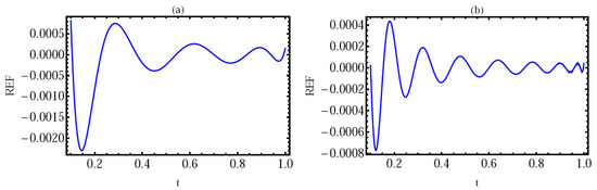
Figure 3. The REF of Example 4 with $\tau =0.1,\alpha =1.98$; at $m=10$ (a) and $m=15$ (b).

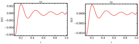
Figure 4. The REF of Example 4 with $\tau =0.01,m=12$; at $\alpha =1.95$ (a) and $\alpha =1.99$ (b).

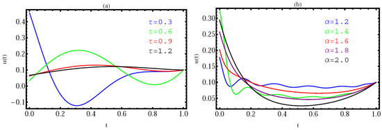
Figure 5. The numerical solution of Example 4, with $m=15$; with different values of $\tau$ (a) and $\alpha$ (b).

Example 5 ((Ikeda system-two delays)).

Consider the Ikeda delay system with two delays which is described in [29]:

$$D^{\alpha }u\left(t\right)=-\kappa u(t-{\tau }_1)+\lambda sin\left(\mu u(t-{\tau }_2)\right),1<\alpha \le 2,$$

(34)

where $\kappa ,\lambda ,\mu ,{\tau }_1$, and ${\tau }_2$ are constants and with:

$$u\left(0\right)=u_0,u\left(1\right)=u_1.$$

(35)

Using the provided method and $m=10$, we arrive at the approximation of the solution as in (25). Using Equation (11), we have

$$\begin{array}{c}\hfill \sum _{n=\lceil \alpha \rceil }^m\sum _{k=\lceil \alpha \rceil }^n{c}_n{w}_{n,k}^{(\nu ,\alpha )}{t}_p^{\nu k-\alpha }=-\kappa \sum _{n=0}^m{c}_n{P}_n^{\nu }(t_p-{\tau }_1)+\lambda sin\left(\mu \sum _{n=0}^m{c}_n{P}_n^{\nu }(t_p-{\tau }_2)\right),\end{array}$$

(36)

with $p=0\left(1\right)8$ where $t_p$ are roots of $P_9^{\nu }\left(t\right)$. Using (25) and (35), we get:

$$\sum _{n=0}^m{(-1)}^n{c}_n=u_0,\sum _{n=0}^m{c}_n=u_1.$$

(37)

Now, solving the system of Equations (36)–(37), we obtain the approximate solution to this model (34).

Here, we define the REF to conduct a full numerical study with the simulation:

$$\mathit{REF}(t,m)=\sum _{n=\lceil \alpha \rceil }^m\sum _{k=\lceil \alpha \rceil }^n{c}_n{w}_{n,k}^{(\nu ,\alpha )}{x}^{\nu k-\alpha }+\kappa \sum _{n=0}^m{c}_n{P}_n^{\nu }(t-{\tau }_1)-\lambda sin\left(\mu \sum _{n=0}^m{c}_n{P}_n^{\nu }(t-{\tau }_2)\right).$$

(38)

Using the provided method, we present a numerical simulation of this model (34) using the suggested approach in Figure 6, Figure 7 and Figure 8 with $\kappa =3,\lambda =24,\mu =1$ and initial values $u_0=u_1=0.1$. In Figure 6, the REF at ${\tau }_1={\tau }_2=0.1,\alpha =1.98$ with $m=10$ (a) and $m=15$ (b) is given. In Figure 7, the REF at ${\tau }_1={\tau }_2=0.01,m=12$ with $\alpha =1.95$ (a) and $\alpha =1.99$ (b) is given. Finally, in Figure 8, the solution at $m=10,\alpha =1.98$; with ${\tau }_1=0.3,0.6,0.9,1.2$ (a) and ${\tau }_2=0.3,0.6,0.9,1.2$ (b) is given. These Figures demonstrate that the solution depends on $\alpha ,{\tau }_1$ and ${\tau }_2$, demonstrating the effectiveness of the numerical technique for solving this issue in fractional derivatives.

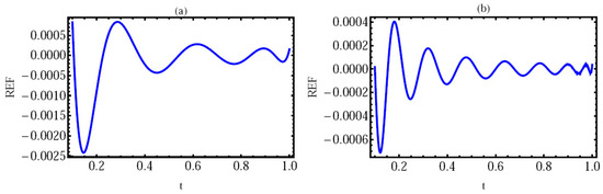
Figure 6. The REF of Example 5 with ${\tau }_1={\tau }_2=0.1,\alpha =1.98$; at $m=10$ (a) and $m=15$ (b).

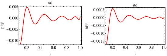
Figure 7. The REF of Example 5 with ${\tau }_1={\tau }_2=0.01,m=12$; at $\alpha =1.95$ (a) and $\alpha =1.99$ (b).

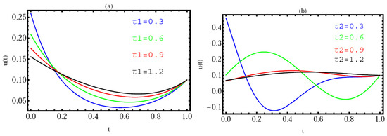
Figure 8. The numerical solution of Example 5, with $m=10,\alpha =1.98$; with different values of ${\tau }_1$ (a) and ${\tau }_2$ (b).

7. Conclusions and Remarks

This work’s primary focus is on presenting fractional Legendre polynomials with states and demonstrating some of their characteristics. In addition, the Legendre SCM is used in this article to solve fractional delay differential equations. The suggested problem is reduced to a system of algebraic equations, which can be solved using an appropriate numerical method, leveraging the properties of the new fractional Legendre polynomials. We examine the convergence analysis, the generated formula’s accuracy, and the approximation of the solution. The numerical simulations show that this approach to applying the Liouville–Caputo derivative is an effective way to solve FDDE. In addition, Only a few shifted fractional Legendre polynomials are required to produce a good outcome. By including new terms in the series, overall error rates can be reduced.

References

- Adel, M.; Srivastava, H.M.; Khader, M.M. Implementation of an accurate method for the analysis and simulation of electrical R-L circuits. Math. Meth. Appl. Sci. 2023, 46, 8362–8371. [Google Scholar] [CrossRef]
- Saadatmandi, A.; Dehghan, M. A new operational matrix for solving fractional-order differential equations. Comput. Math. Appl. 2010, 59, 1326–1336. [Google Scholar] [CrossRef]
- Basti, B.; Hammami, N.; Berrabah, I.; Nouioua, F.; Djemiat, R.; Benhamidouche, N. Stability analysis and existence of solutions for a modified SIRD model of Covid-19 with fractional derivatives. Symmetry 2021, 13, 1431. [Google Scholar] [CrossRef]
- Khoojine, A.S.; Mahsuli, M.; Shadabfar, M.; Hosseini, V.R.; Kordestani, H. A proposed fractional dynamic system and Monte Carlo-based back analysis for simulating the spreading profile of Covid. Eur. Phys. J. Spec. Top. 2022, 19, 1–11. [Google Scholar]
- Butt, A.I.K.; Imran, M.; Batool, S.; Nuwairan, M.A.L. Theoretical analysis of a Covid-19 CF-fractional model to optimally control the spread of Pandemic. Symmetry 2023, 15, 380. [Google Scholar] [CrossRef]
- Adel, M.; Khader, M.M.; Ahmad, H.; Assiri, T.A.; Batool, S.; Nuwairan, M.A.L. Approximate analytical solutions for the blood ethanol concentration system and predator-prey equations by using variational iteration method. Aims Math. 2023, 8, 19083–19096. [Google Scholar] [CrossRef]
- Abd-Elhameed, W.M. New Galerkin operational matrix of derivatives for solving Lane-Emden singular-type equations. Eur. Phys. J. Plus 2015, 130, 52. [Google Scholar] [CrossRef]
- Khan, M.A.; Atangana, A. Modeling the dynamics of novel Coronavirus (2019-nCoV) with fractional derivative. Alex. Eng. J. 2020, 56, 2379–2389. [Google Scholar] [CrossRef]
- Dokuyucu, M.A.; Celik, E.; Bulut, H.; Baskonus, H.M. Cancer treatment model with the Caputo-Fabrizio fractional derivative. Eur. Phys. J. Plus 2018, 133, 92. [Google Scholar] [CrossRef]
- Dokuyucu, M.A.; Celik, E. Analyzing a novel coronavirus model (COVID-19) in the sense of Caputo-Fabrizio fractional operator. Appl. Comput. Math. 2021, 20, 49–69. [Google Scholar]
- Oldham, K.B.; Spanier, J. The Fractional Calculus; Academic Press: New York, NY, VSA, 1974. [Google Scholar]
- Podlubny, I. Fractional Differential Equations; Academic Press: New York, NY, VSA, 1999. [Google Scholar]
- Jafari, H.; Momani, S. Solving fractional diffusion and wave equations by modified homotopy perturbation method. Phys. Lett. 2007, 370, 388–396. [Google Scholar] [CrossRef]
- Adel, M.; Khader, M.M.; Assiri, T.A.; Kallel, W. Simulating Covid-19 model research using a multidomain spectral relaxation technique. Symmetry 2023, 15, 931. [Google Scholar] [CrossRef]
- Srivastava, H.M.; Kilbas, A.A.; Trujillo, J.J. Theory and Application of Fractional Differential Equations; Elsevier: Amsterdam, The Netherlands, 2006. [Google Scholar]
- Khader, M.M. An efficient class of discrete finite difference/element scheme for solving the fractional reaction sub-diffusion equation. Math. Methods Appl. Sci. 2023, 46, 10512–10526. [Google Scholar] [CrossRef]
- Adel, M.; Khader, M.M.; Algelany, S. High-dimensional chaotic Lorenz system: Numerical treated using Changhee polynomials of the Appell type. Fractal Fract. 2023, 7, 398. [Google Scholar] [CrossRef]
- Kazem, S.; Abbasbandy, S.; Kumar, S. Fractional-order Legendre functions for solving fractional-order differential equations. Appl. Math. Model. 2013, 37, 5498–5510. [Google Scholar] [CrossRef]
- Ramadan, M.A. Spline solution of first order delay differential equation. J. Egypt. Math. Soc. 2005, 1, 7–18. [Google Scholar]
- Ramdan, M.A.; Shrif, M.N. Numerical solution of a system of first order delay differential equations using spline functions. Int. J. Comput. Math. 2006, 83, 925–937. [Google Scholar] [CrossRef]
- Miller, K.S.; Ross, B. An Introduction to the Fractional Calculus and Fractional Differential Equations; John Wiley and Sons: New York, NY, USA, 1993. [Google Scholar]
- Odibat, Z.M.; Shawagfeh, N.T. Generalized Taylor’s formula. Appl. Math. Comput. 2007, 186, 286–293. [Google Scholar] [CrossRef]
- Bell, W.W. Special Functions for Scientists and Engineers; Great Britain, Butler and Tanner Ltd.: Frome, UK; London, UK, 1968. [Google Scholar]
- Khader, M.M.; Sweilam, N.H. Approximate solutions for the fractional advection-dispersion equation using Legendre pseudo-spectral method. Comp. Appl. Math. 2014, 33, 739–750. [Google Scholar] [CrossRef]
- Li, B.; Liu, S.; Cui, J.; Li, J. A simple Predator-Prey population model with rich dynamics. Appl. Sci. 2016, 6, 151. [Google Scholar] [CrossRef]
- Bhalekar, S. Stability and bifurcation analysis of a generalized scalar delay differential equation. Chaos Interdiscip. J. Nonlinear Sci. 2016, 26, 084306. [Google Scholar] [CrossRef] [PubMed]
- Lu, J.-G. Chaotic dynamics of the fractional-order Ikeda delay system and its synchronization. Chin. Phys. 2006, 15, 301. [Google Scholar]
- Parand, K.; Delkhosh, M. Operational matrices to solve nonlinear Volterra-Fredholm IDEs of multi-arbitrary order. Gazi Univ. J. Sci. 2016, 29, 895–907. [Google Scholar]
- Bhalekar, S. Analyzing the stability of a delay differential equation involving two delays. Pramana-J. Phys. 2019, 93, 24. [Google Scholar] [CrossRef]
Disclaimer/Publisher’s Note: The statements, opinions and data contained in all publications are solely those of the individual author(s) and contributor(s) and not of MDPI and/or the editor(s). MDPI and/or the editor(s) disclaim responsibility for any injury to people or property resulting from any ideas, methods, instructions or products referred to in the content. |
© 2023 by the authors. Licensee MDPI, Basel, Switzerland. This article is an open access article distributed under the terms and conditions of the Creative Commons Attribution (CC BY) license (https://creativecommons.org/licenses/by/4.0/).