Robot Manipulator Control Using a Robust Data-Driven Method

Abstract

Robotic manipulators with diverse structures find widespread use in both industrial and medical applications. Therefore, designing an appropriate controller is of utmost importance when utilizing such robots. In this research, we present a robust data-driven control method for the regulation of a 2-degree-of-freedom (2-DoF) robot manipulator. The nonlinear dynamic model of the 2-DoF robot arm is linearized using Koopman theory. The data mode decomposition (DMD) method is applied to generate the Koopman operator. A fractional sliding mode control (FOSMC) is employed to govern the data-driven linearized dynamic model. We compare the performance of Koopman fractional sliding mode control (KFOSMC) with conventional proportional integral derivative (PID) control and FOSMC prior to linearization by Koopman theory. The results demonstrate that KFOSMC outperforms PID and FOSMC in terms of high tracking performance, low tracking error, and minimal control signals.

1. Introduction

Robotic manipulators are highly utilized in various industries, such as automotive and medical. These robots are in high demand and are often deployed in conditions where they encounter external disturbances. Therefore, designing a suitable control method is the most critical aspect of the robotics design process. Many control methods are applied to robot manipulators to guide them along the desired trajectory, including the PID controller [1,2,3,4], sliding mode control [5,6,7], and fuzzy PID control [8,9,10], among others. These mentioned control methods depend on the dynamic model of the robot manipulator. However, designing certain control methods, such as the model predictive controller and conventional sliding mode control, requires an accurate dynamic model. Data-driven methods are strong approaches that can approximate the dynamic model to generate precise model characteristics.

Carron et al. [11] have introduced a model-based control method that utilizes data acquired from actual operations to enhance the robotic arm’s model and tracking performance. The foundations of this approach are inverse dynamics feedback linearization and a data-driven error model, which are incorporated into a formulation for model predictive control. They also demonstrated how incorporating a Gaussian process into a nominal model can enable offset-free tracking. To achieve trajectory tracking control of the manipulator, the Gaussian process feedback linearization approach, based on the updating of the event-triggered model, is applied in a manipulator system with three degrees of freedom [12]. To address the challenge of extensive Gaussian process regression computation with large data samples, sparse Gaussian process regression is employed for real-time manipulator trajectory tracking. It should be noted that the controllers proposed in [11,12] lack robustness against external disturbances, and it is important to compare these proposed methods with conventional controllers to assess their performance.

The Koopman theory is a robust method for data-driven control techniques. It has the capability to linearize complex nonlinear dynamic models. Several researchers have incorporated the Koopman theory into their studies to achieve enhanced control performance [13,14,15,16,17]. However, a critical aspect of applying the Koopman theory is the design of the Koopman operator. The Dynamic Mode Decomposition (DMD) method is one of the valuable techniques that can be employed to construct the Koopman operator. Extended Dynamic Mode Decomposition (EDMD), introduced by Junker et al. [18], allows for the approximation of a nonlinear dynamical system as a linear model. Given the widespread use of linear system descriptions in control engineering applications, this technique is particularly well suited for such purposes. Junker et al. [18] conducted a simulated analysis of the prediction performance of the learned EDMD models using academic examples. They demonstrated how crucial system properties, such as stability, controllability, and observability, are reflected in the EDMD model. This reflection is a critical prerequisite for a successful control design process. Furthermore, they presented experimental findings on a mechatronic test bench and evaluated the applicability of their results to the control engineering design procedure.

Within the realm of data-driven Koopman operator-based nonlinear robotic systems, Shi and Karydis [19] propose ACD-EDMD, a novel approach for the Analytical Construction of Dictionaries of Appropriate Lifting Functions. The primary discovery in this study is that Hermite polynomial-based lifting functions can be constructed by leveraging knowledge of the fundamental topological spaces of the nonlinear system. They demonstrate that when observables are bounded and weighted, the suggested approach produces dictionaries with proven completeness and convergence guarantees that are easy to implement. ACD-EDMD is evaluated using various nonlinear robotic systems, including both simulated and real hardware experiments. To address the limitation of this approach and extract the leading Koopman eigenvalues, eigenfunctions, and modes of the unforced system, Williams et al. [20] describe a modified version of EDMD that accounts for the effects of actuation. They illustrate the effectiveness of this method using two examples: the Duffing oscillator and a lattice Boltzmann code approximating the Fitzhugh–Nagumo partial differential equation, which demonstrates Koopman mode and eigenvalue computation under (quasi)-periodic forcing. However, while the Koopman theory offers numerous advantages, its limitations can be described as follows:

1-

Control constraints: Koopman control may not easily accommodate control constraints, such as safety limits on system states or control inputs. Ensuring that the control strategy remains within these constraints can be challenging.

2-

Computational complexity: solving the Koopman control problem can be computationally intensive, particularly for high-dimensional systems. Real-time control implementation may be limited by computational constraints.

In recent years, the emergence of fractional calculus has significantly reshaped the landscape of mathematical analysis and its applications. Fractional calculus extends traditional notions of differentiation and integration to non-integer orders, introducing a powerful framework for modeling complex systems with long-range dependence, memory effects, and anomalous diffusion. In this paper, we incorporate the principles of fractional calculus into our research, leveraging its mathematical richness to provide deeper insights into sliding mode control. By embracing fractional calculus, our aim is to enhance control accuracy, improve stability, bolster robustness, and achieve high tracking performance.

This research makes the following contributions:

1-

The application of Koopman theory to linearize the nonlinear dynamics of the 2-DoF robot manipulator.

2-

The use of the DMD method to obtain the Koopman operator.

3-

The proposal of a fractional sliding mode control to regulate the linearized dynamics model based on Koopman’s theory.

4-

Implementation of conventional PID and FOSMC controllers to assess the performance of the proposed control method.

The rest of the paper is organized as follows: Section 2 describes the nonlinear model of the 2-DoF robot manipulator. Section 3 introduces the PID controller. Section 4 discusses FOSMC. Section 5 delves into Koopman theory. Section 6 explains the DMD method. Section 7 demonstrates KFOSMC. Section 8 presents simulation results and Section 9 concludes the paper.

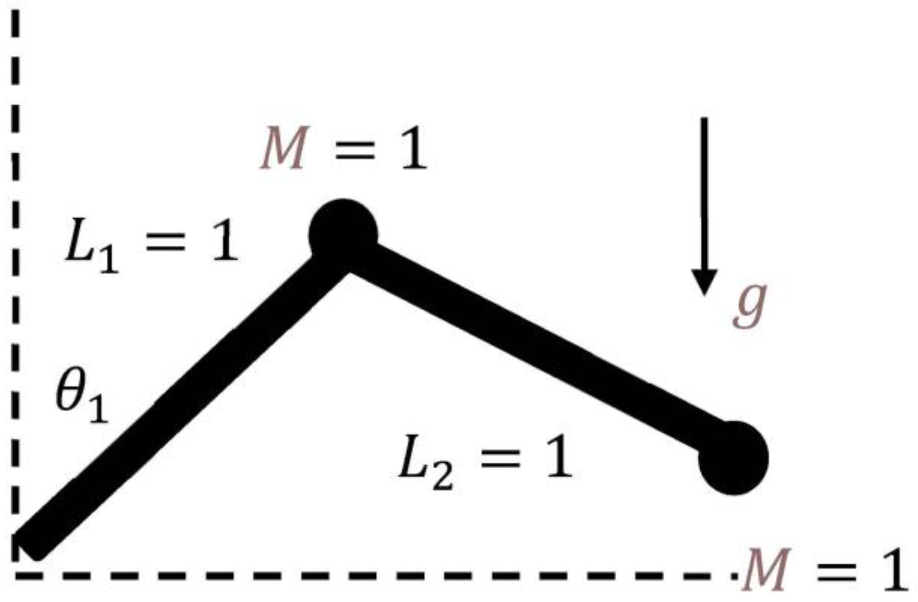
2. Dynamic Model of 2-DoF Robot Manipulator

Robots have the potential to enhance productivity, efficiency, product consistency, and quality in a variety of situations. Unlike humans, robots do not experience boredom and can tirelessly perform repetitive tasks until they wear out. Robot manipulators have numerous applications, including exoskeleton robots [21] and refueling robots [22].

The following example illustrates the dynamic modeling of a 2-degree-of-freedom (2-DOF) robot manipulator [23]:

$$M\left(q\right)\ddot{q}+N\left(q,\dot{q}\right)\dot{q}+G\left(q\right)=\tau$$

(1)

where $q,\dot{q},\ddot{q}∊R^2$ represent the position, velocity, and acceleration of the joints, respectively, and $M\left(q\right)∊R^{2\times 2}$ is known as the generalized inertia matrix, $N(q,\dot{q})∊R^{2\times 2}$ is the vector of Coriolis and centrifugal forces, $G\left(q\right)∊R^{2\times 1}$ is the gravitational vector, and $\tau ∊R^{2\times 1}$ is the joint torques. $M\left(q\right)$, $N(q,\dot{q})$ and $G\left(q\right)$ are given in Appendix A. Equation (1) can be defined as:

$$\ddot{q}=-M^{-1}\left(q\right)N\left(q,\dot{q}\right)\dot{q}-M^{-1}\left(q\right)G\left(q\right)+M^{-1}\left(q\right)\tau$$

(2)

The 2DoF robot manipulator structure is shown in Figure 1. It is possible to rearrange the dynamic equation for a 2-DOF robot manipulator as follows:

$$\ddot{q}=-B\dot{q}-CG\left(q\right)+u$$

(3)

where $B=M^{-1}\left(q\right)N\left(q,\dot{q}\right)$, $C=M^{-1}\left(q\right)$, and $u=M^{-1}\left(q\right)\tau$. The definition of Equation (4) where $\Delta B$ and $\Delta C$ are uncertainty symbols is:

$$\ddot{q}=-(B+\Delta B)\dot{q}-(C+\Delta C)G\left(q\right)+u$$

(4)

Equation (4) can be introduced as:

$$\ddot{q}=-B\dot{q}-CG\left(q\right)+u+d\left(t\right)$$

(5)

where $d\left(t\right)=-\Delta B\dot{q}-CG\left(q\right)$, which includes unmodeled dynamics and external disturbances.

Problem Statement:

The primary objective of this research is to design a control system that achieves asymptotic stabilization for the 2-DoF robot manipulator. Asymptotic stabilization implies that the robot manipulator should track the desired trajectory, denoted as$q_d\left(t\right)$, and approach it as time t approaches infinity (t → +∞), while maintaining bounded values for its state variables and control inputs. In mathematical terms, the problem can be formally stated as follows:

Design a control law u(t) such that the system’s state q(t) approaches the desired trajectory $q_d\left(t\right)$ as t → +∞, while ensuring that $q\left(t\right)$, $q_d\left(t\right)$, and u(t) remain bounded and the tracking error $q\left(t\right)$ − $q_d\left(t\right)$ converges to zero.

The solution to this problem involves the development of a control algorithm, which may include elements such as trajectory planning, feedback control, and disturbance rejection, while considering the physical limitations and constraints of the robot manipulator.

Addressing this problem is crucial for enhancing the performance and precision of 2-DoF robot manipulators in various applications, such as manufacturing, automation, and robotics, where accurate trajectory tracking is essential for task execution and safety. In the subsequent sections, we will delve into the control strategies and approaches employed to tackle this problem, along with simulation results and experimental validations.

3. PID Control Model

The PID controller has been highly used in industrial companies due to its easy implementation and low cost. The PID controller can be defined as:

$$u_{PID}=K_{p}e\left(t\right)+K_i{\int }_0^{t}e\left(\tau \right)d\tau +K_d\frac{de\left(t\right)}{dt}$$

(6)

where $K_p,K_i$, and $K_d$ are proportional, integral, and derivative parameters. Moreover, the tracking error can be defined as:

$$e\left(t\right)=q_d-q$$

(7)

where $q_d$ is desired trajectory tracking. The main drawbacks of the PID controller are that it is not robust against external disturbances and has low trajectory tracking.

4. Fractional Order Sliding Mode Control

FOSMC is a robust control method against external perturbations and demonstrates high tracking performance. Its primary advantage, when compared to conventional sliding mode control, lies in its ability to incorporate fractional derivatives or integrals of the error. The key aspect of FOSMC design involves selecting the fractional sliding mode surface as:

$$s\left(t\right)=\dot{e}\left(t\right)+\alpha D^{\mu }e\left(t\right)+\beta D^{-\mu }e\left(t\right)$$

(8)

where $\alpha$ and $\beta$ are positive constants and D is the Grunwald–Letnikov fractional operator. The Grunwald–Letnikov fractional derivative of the function e(t) with respect to t is given as $D_t^{\mu }e\left(t\right)={lim}_{h\to 0}{h}^{-\mu }\sum _{k=0}^n{(-1)}^k\left(\begin{array}{c}\mu \\ k\end{array}\right)f\left(e\left(t\right)-kh\right)$, where the fractional order operator parameters $\mu$ and $k$ will be obtained by $\left(\begin{array}{c}\mu \\ k\end{array}\right)=\frac{\mu \left(\mu -1\right)\left(\mu -2\right)\dots (\mu -k+1)}{k!}=\frac{\Gamma \left(\mu +1\right)}{k!\Gamma \left(\mu -k+1\right)}$.

The FOSMC contains two control sections: equivalent control and reaching control law. The equivalent control method can be obtained by equaling the derivative of the sliding mode surface to zero. Taking derivative from Equation (8) results in:

$$\dot{s}\left(t\right)=\ddot{e}\left(t\right)+\alpha \mu D^{\mu +1}e\left(t\right)-\beta \mu D^{-\mu +1}e\left(t\right)$$

(9)

Taking double derivative from Equation (7) and substituting into Equation (9) produces:

$$\dot{s}\left(t\right)={\ddot{q}}_d-\ddot{q}+\alpha \mu D^{\mu +1}e\left(t\right)-\beta \mu D^{-\mu +1}e\left(t\right)$$

(10)

Substituting Equation (5) into Equation (10) generates:

$$\dot{s}\left(t\right)={\ddot{q}}_d+B\dot{q}+CG\left(q\right)-u-d\left(t\right)+\alpha \mu D^{\mu +1}e\left(t\right)-\beta \mu D^{-\mu +1}e\left(t\right)$$

(11)

By equaling Equation (11) and d(t) to zero, the equivalent control can be obtained as:

$$u_{eq}={\ddot{q}}_d+B\dot{q}+CG\left(q\right)+\alpha \mu D^{\mu +1}e\left(t\right)-\beta \mu D^{-\mu +1}e\left(t\right)$$

(12)

The equivalent control solely is not able to suppress the external disturbances. Therefore, a reaching control law will be implemented to solve that problem. The reaching control law is introduced as [25]:

$$u_r=K_{r}s\left(t\right)$$

(13)

Therefore, the FOSMC is defined as:

$$u_{FOSMC}\left(t\right)=u_{eq}\left(t\right)+u_r\left(t\right)$$

(14)

The proposed control method’s stability can be proved by using the Lyapunov theory as:

$$V\left(t\right)=\frac{1}{2}{s}^T\left(t\right)s(t)$$

(15)

The condition for stability satisfaction is as follows:

$$\dot{V}\left(t\right)=s^T\left(t\right)\dot{s}\left(t\right)<0$$

(16)

Substituting Equation (11) into Equation (16) produces:

$$\dot{V}\left(t\right)=s^T\left(t\right)({\ddot{q}}_d+B\dot{q}+CG\left(q\right)-u+\alpha \mu D^{\mu +1}e\left(t\right)-\beta \mu D^{-\mu +1}e\left(t\right))$$

(17)

Substituting Equation (14) into Equation (17) introduces:

$$\dot{V}\left(t\right)=s^T\left(t\right)({\ddot{q}}_d+B\dot{q}+CG\left(q\right)-u_{eq}\left(t\right)-u_r\left(t\right)+\alpha \mu D^{\mu +1}e\left(t\right)-\beta \mu D^{-\mu +1}e\left(t\right))$$

(18)

Substituting Equation (12) into Equation (18) results in:

$$\dot{V}\left(t\right)=s^T\left(t\right)({\ddot{q}}_d+B\dot{q}+CG\left(q\right)-{\ddot{q}}_d-B\dot{q}-CG\left(q\right)-\alpha \mu D^{\mu +1}e\left(t\right)+\beta \mu D^{-\mu +1}e\left(t\right)-u_r\left(t\right)+\alpha \mu D^{\mu +1}e\left(t\right)-\beta \mu D^{-\mu +1}e\left(t\right))$$

(19)

Simplifying Equation (19) demonstrates:

$$\dot{V}\left(t\right)=s^T\left(t\right)(-u_r\left(t\right))$$

(20)

Substituting Equation (13) into Equation (20) produces:

$$\dot{V}\left(t\right)=s^T\left(t\right)(-K_{r}s(t\left)\right)$$

(21)

Equation (21) satisfies the condition in Equation (16). Therefore, the proposed controller is stable.

5. Koopman Theory

The key to successfully solving a nonlinear dynamical system, according to the Koopman operator theory, is to convert the nonlinear system’s original form into an infinite dimensional state space, resulting in a linear system [26]. Consider a continuous-time dynamical system as $\dot{x}=f\left(x\right).$ The discrete time definition of the dynamic is [27]:

$$x_{k+1}=F\left(x_k\right)$$

(22)

where F is characterized by:

$$F\left(x\left(t_0\right)\right)=x\left(t_0\right)+{\int }_{t_0}^{t_0+t}f\left(x\left(\tau \right)\right)d\tau$$

(23)

The dynamics of the original system become linear when the dynamics of a finite-dimensional nonlinear system is transferred to an infinite-dimensional function space. In an infinite-dimensional Hilbert space, g is an observable and a real-valued scalar measurement function. Based on this observable, the Koopman operator generates as follows:

$$Kg=g\circ F$$

(24)

A continuous system can be utilized to implement smooth dynamics.

$$\frac{d}{dt}g\left(x\right)=Kg\left(x\right)=\nabla g\left(x\right).f\left(x\right)$$

(25)

in which K is the Koopman operator. due to the Koopman operator’s unlimited dimensions, which is important yet troublesome for operation and representation. Applied Koopman analysis roughly approximates the evolution of a subspace covered by a limited number of measurement functions rather than detailing the development of all measurement functions in a Hilbert space. By constraining the operator to an invariant subspace, the Koopman operator may be represented as a matrix with limited dimensions. Any combination of the Koopman operator’s eigenfunctions can cover a Koopman invariant subspace [27]. When the Koopman model’s eigenfunction $\phi \left(x\right)$ satisfies eigenvalue λ:

$$\lambda \phi \left(x\right)=\phi \left(F\left(x\right)\right)$$

(26)

A Koopman eigenfunction $\phi \left(x\right)$ is satisfied in continuous time.

$$\frac{d}{dt}\phi \left(x\right)=\lambda \phi \left(x\right)$$

(27)

To approximate the Koopman operator, a finite-dimensional approximation is needed on the application side. The DMD technique is one way that can estimate the Koopman operator [27]. Here are some conditions under which it is acceptable to use the linearized model obtained by Koopman theory:

• Local linearity: the Koopman theory linearization is typically valid only in the vicinity of equilibrium points or limit cycles of the nonlinear system. Therefore, it is acceptable to use the linearized model when you are interested in studying the system’s behavior near these points.
• Small perturbations: the linearized model is a good approximation when the system experiences small perturbations around a stable equilibrium. In such cases, the linearized model can provide insights into the stability and local behavior of the system.
• Short-time predictions: if you are interested in short-term predictions or analyzing the system’s behavior over a relatively small time interval, the linearized model can be acceptable. It often provides accurate predictions for short time horizons.
• Reduced-order modeling: Koopman theory can be used to reduce the dimensionality of a high-dimensional nonlinear system, creating a lower-dimensional linearized model that retains important dynamics. This can be valuable for simplifying complex systems while preserving critical behaviors.

6. DMD Method

DMD uses a robust numerical technique to approximate the Koopman operator.

$$X^{\prime }\approx AX$$

(28)

where $X^{\prime }$ is time shift of matrix X as:

$$X=\left[\begin{array}{ccc}{x}_1& x_2& \dots \dots .\end{array}\right]$$

Equation (28) may be used to determine A as follows:

$$A=X^{\prime }{X}^{+}$$

(29)

where the Moore–Penrose pseudoinverse is represented by +. Because a normal calculation utilizing A would need a substantial amount of processing because of its enormous n, we may utilize singular value decomposition (SVD) on the snapshots to identify the dominant characteristics of the pseudoinverse of X [28].

$$X\approx U\Sigma V*$$

(30)

where $U∊R^{n\times r}$, $\Sigma ∊R^{r\times r}$, $V∊R^{n\times r}$, and * demonstrate the conjugate transpose. SVD’s reduced rank for approximating X is r. The eigenvectors can be defined as:

$$\mathrm{\Phi }=X^{\prime }V{\Sigma }^{-1}W$$

(31)

where W is eigenvectors of full rank system dynamic systems.

$$W=X^{\prime }V{\Sigma }^{-1}\mathrm{\Phi }$$

(32)

Let λ be eigenfunction, then we will have:

$$KW=\lambda W$$

(33)

where K is the Koopman operator.

The demonstration of the linearized dynamic model is as follows:

$$\frac{d}{dt}y=Ky+u$$

(34)

where y is the state variable of the linearized system.

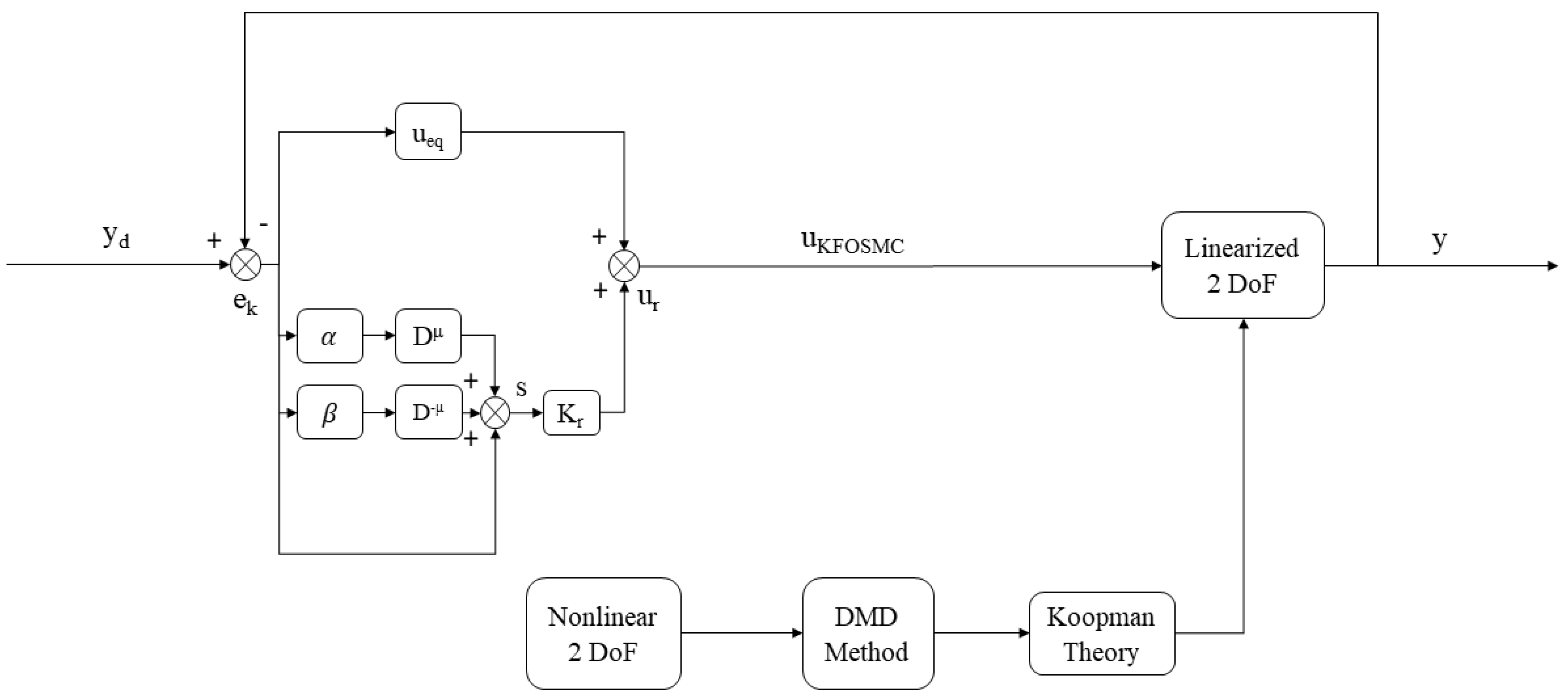
7. Koopman Fractional Sliding Mode Control

The proposed control method block diagram is shown in Figure 2. The fractional sliding mode surface for the linearized dynamic model by Koopman theory can be defined as:

$$s_k\left(t\right)=e_k\left(t\right)+\alpha D^{\mu }{e}_k\left(t\right)+\beta D^{-\mu }{e}_k\left(t\right)$$

(35)

where the e_k is the tracking error as:

$$e_k\left(t\right)=y_d-y$$

(36)

where $y_d$ is the desired trajectory.

Taking the derivative of the fractional sliding mode results in the following equation:

$${\dot{s}}_k\left(t\right)={\dot{e}}_k\left(t\right)+\alpha {\mu D}^{\mu +1}{e}_k\left(t\right)-\beta {\mu D}^{-\mu +1}{e}_k\left(t\right)$$

(37)

Taking derivative from Equation (36) and substituting into Equation (37) produces:

$${\dot{s}}_k\left(t\right)={\dot{y}}_d-\dot{y}+\alpha {\mu D}^{\mu +1}{e}_k\left(t\right)-\beta {\mu D}^{-\mu +1}{e}_k\left(t\right)$$

(38)

Substituting Equation (34) into Equation (38) introduces:

$${\dot{s}}_k\left(t\right)={\dot{y}}_d-Ky-u+\alpha {\mu D}^{\mu +1}{e}_k\left(t\right)-\beta {\mu D}^{-\mu +1}{e}_k\left(t\right)$$

(39)

Equaling Equation (39) to zero and simplifying it produces:

$$u_{eq}\left(t\right)={\dot{y}}_d-Ky+\alpha {\mu D}^{\mu +1}{e}_k\left(t\right)-\beta {\mu D}^{-\mu +1}{e}_k\left(t\right)$$

(40)

The equivalent control is not able to suppress external disturbances. The reaching control can be defined as:

$$u_{rk}\left(t\right)=K_{rk}{s}_k\left(t\right)$$

(41)

where $K_{rk}$ is the reaching control gain that is positive constant.

The KFOSMC is defined as:

$${u_{KFOSMC}\left(t\right)=u}_{rk}\left(t\right)+u_{eq}\left(t\right)$$

(42)

The stability of the proposed control method can be proved by using Lyapunov theory as:

$$V\left(t\right)=\frac{1}{2}{s}_k^T(t)s_k(t)$$

(43)

Taking derivative from Equation (43) produces:

$$\dot{V}\left(t\right)=s_k^T(t){\dot{s}}_k(t)$$

(44)

Substituting Equation (39) into Equation (44) produces:

$$\dot{V}\left(t\right)=s_k^T(t)({\dot{y}}_d-Ky-u+\alpha {\mu D}^{\mu +1}{e}_k\left(t\right)-\beta {\mu D}^{-\mu +1}{e}_k\left(t\right))$$

(45)

Substituting Equation (42) into Equation (45) results in:

$$\dot{V}\left(t\right)=s_k^T(t)({\dot{y}}_d-Ky{-u}_{rk}\left(t\right)-u_{eq}(t)+\alpha {\mu D}^{\mu +1}{e}_k\left(t\right)-\beta {\mu D}^{-\mu +1}{e}_k\left(t\right))$$

(46)

Substituteing Equation (40) into Equation (46) introduces:

$$\dot{V}\left(t\right)=s_k^T(t)({\dot{y}}_d-Ky{-u}_{rk}\left(t\right)-{\dot{y}}_d+Ky-\alpha {\mu D}^{\mu +1}{e}_k\left(t\right)+\beta {\mu D}^{-\mu +1}{e}_k\left(t\right)+\alpha {\mu D}^{\mu +1}{e}_k\left(t\right)-\beta {\mu D}^{-\mu +1}{e}_k\left(t\right))$$

(47)

Simplifying Equation (47) results in:

$$\dot{V}\left(t\right)=s_k^T(t)\left({-u}_{rk}\left(t\right)\right)$$

(48)

Substituting Equation (41) into Equation (48) produces:

$$\dot{V}\left(t\right)=s_k^T(t)(-K_{rk}{s}_k\left(t\right))$$

(49)

Equation (49) demonstrates that the proposed control method is stable.

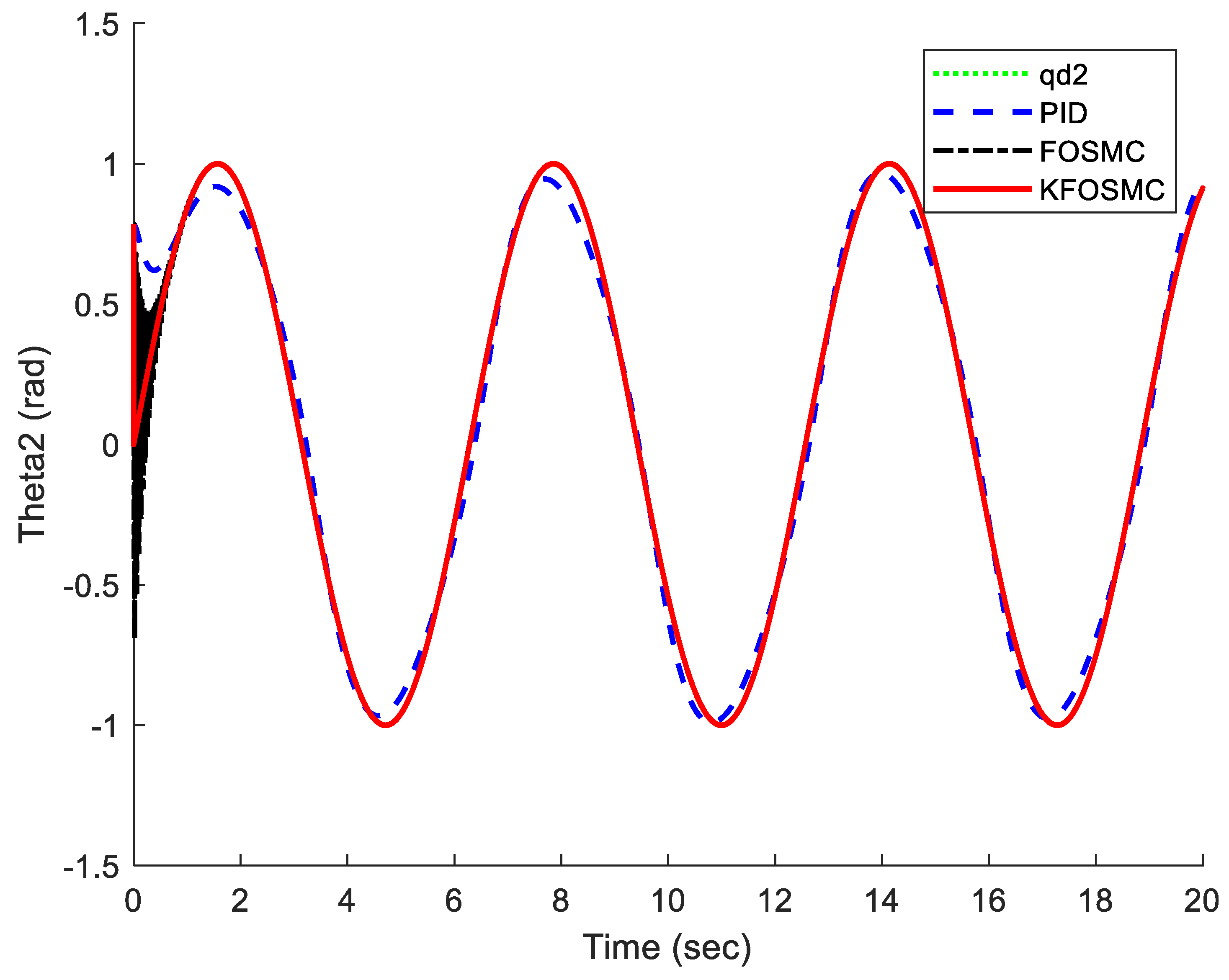
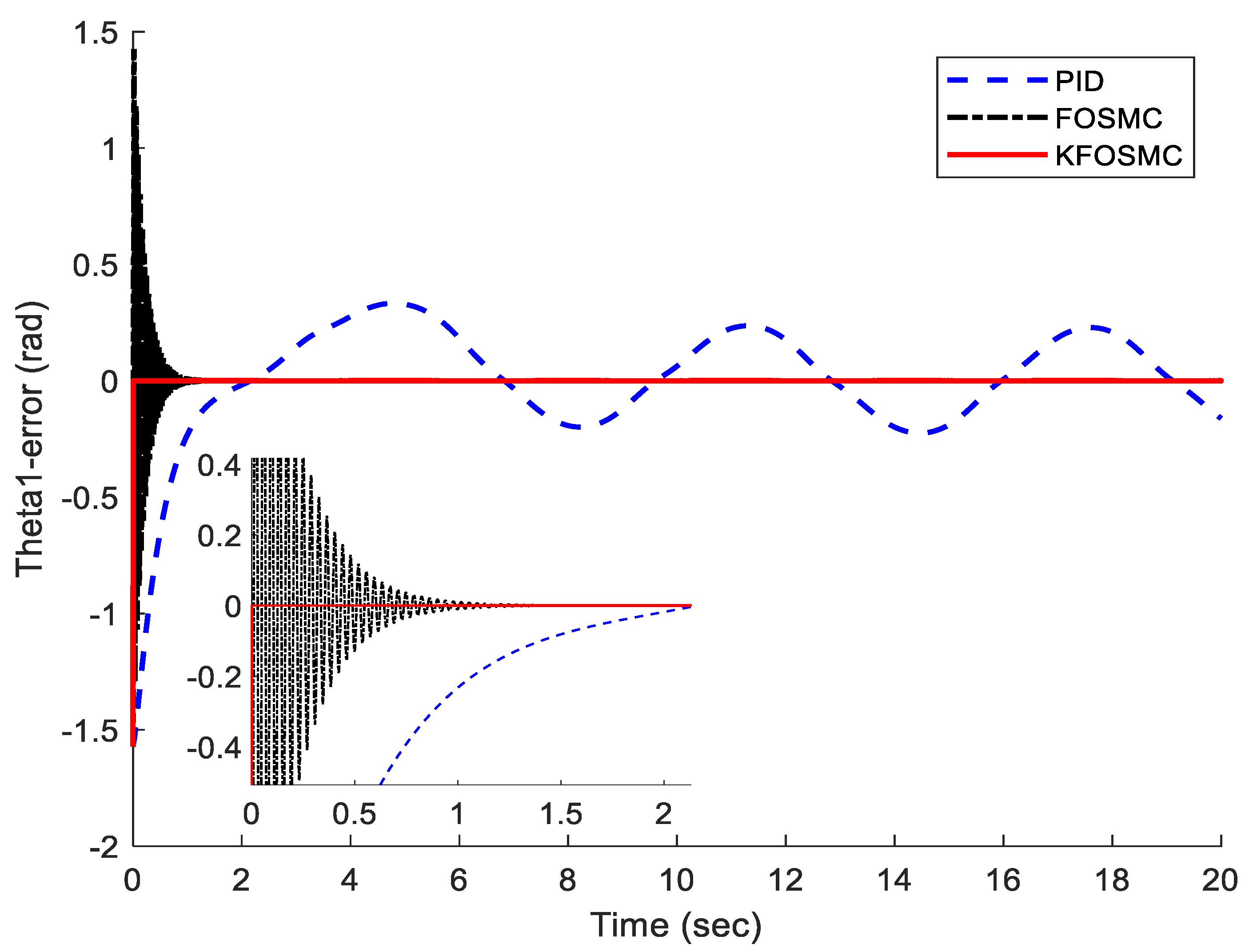
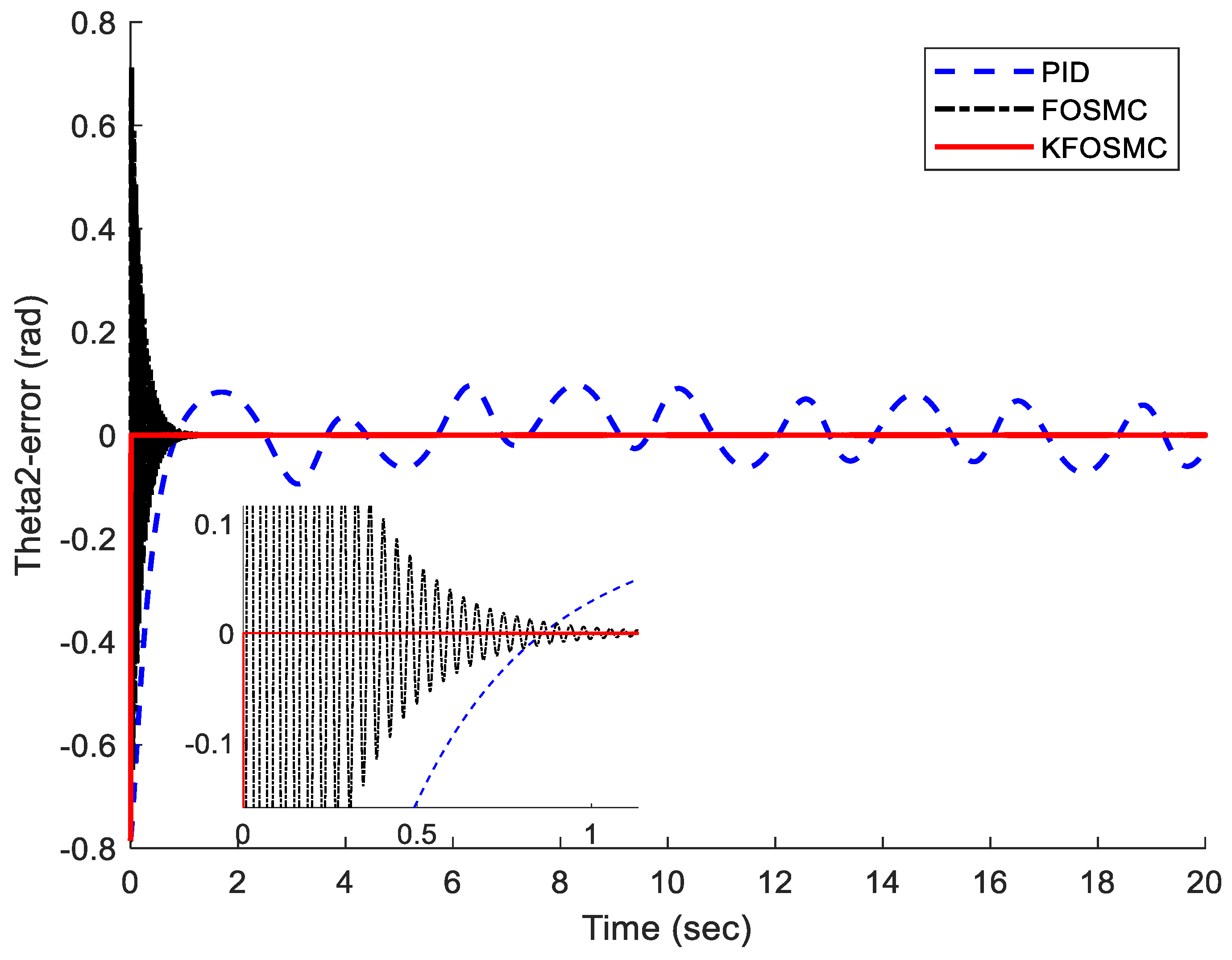
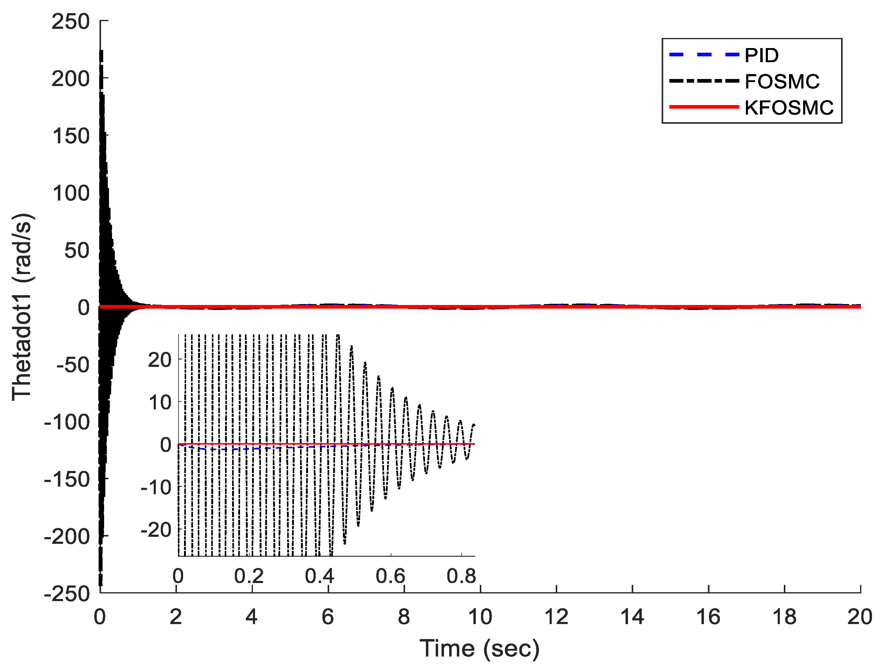
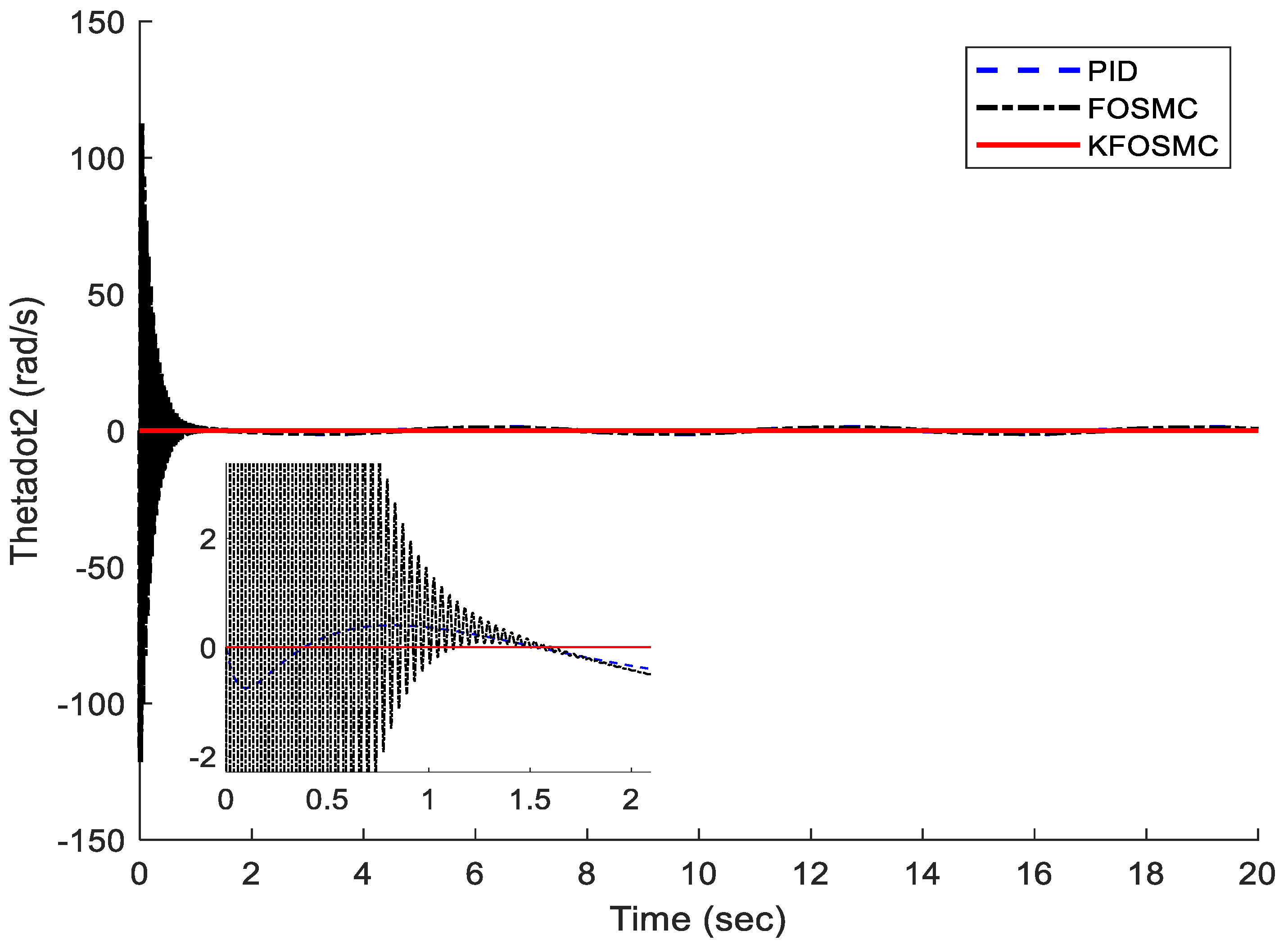
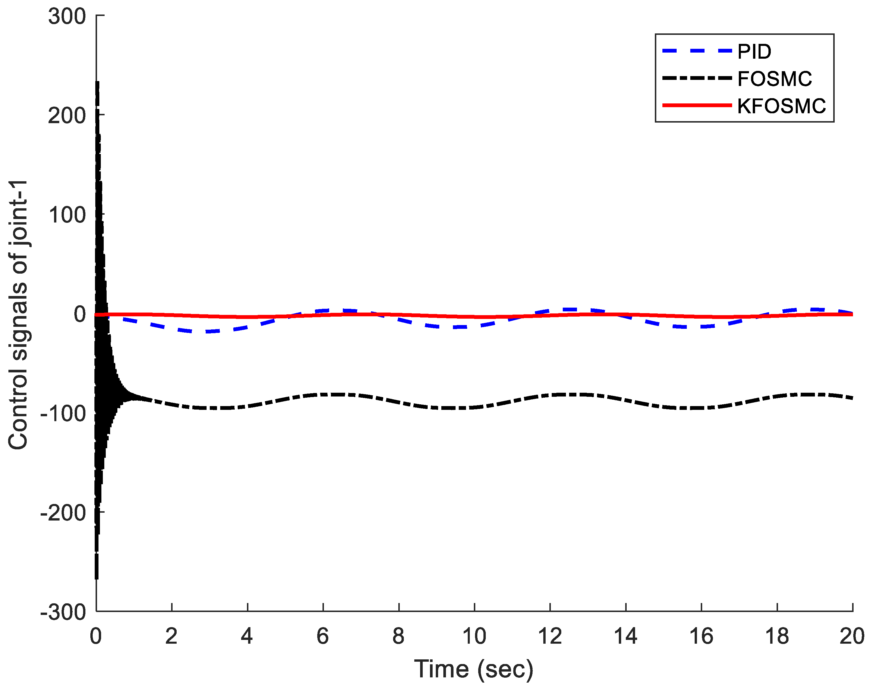
8. Simulation Results

We simulated three controllers to show the performance of the proposed control method. The simulation was conducted in Matlab and using ode 45 order. The time span is [0 20]. The robot’s specifications are $M_1=M_2=L_1=L_2=1$ and $g=9.81 \mathrm{m}/\mathrm{s}$. The PID controller parameters are selected as $K_p=diag\left\{\mathrm{40,40}\right\},K_i=diag\left\{\mathrm{10,10}\right\}$, and $K_d=diag\left\{\mathrm{20,20}\right\}$. The FOSMC controller parameters are chosen as $K_r=10,\alpha =10,\beta =5$, and $\mu =0.75$, with the KFOSMC parameters being the same as FOSMC. These parameters were obtained through the designer experiences and trial–error. The desired trajectory tracking is $q_d=y_d=\mathrm{s}\mathrm{i}\mathrm{n}(t)$. The initial conditions of joints are $q_1=\frac{\pi }{2},q_2=\frac{\pi }{4}$. The linearized Koopman operator is obtained as:

$$K=\left[\begin{array}{ccc}0.9974& 0.1039& \begin{array}{cc}2.76e-04& -0.0019\end{array}\\ -0.0696& 0.9945& \begin{array}{cc}-0.0011& 0.0029\end{array}\\ \begin{array}{c}2.06e-13\\ 1.7076e-15\end{array}& \begin{array}{c}-2.4197e-13\\ -5.2477e-15\end{array}& \begin{array}{cc}\begin{array}{c}-1.7426e-13\\ -1.1075e-14\end{array}& \begin{array}{c}-1.7535e-13\\ 1.6853e-14\end{array}\end{array}\end{array}\right]$$

Figure 3 shows the trajectory tracking of joints 1 and 2 under PID, FOSMC, and KFOSMC. It demonstrates that the KFOSMC has better trajectory tracking performance in comparison with PID and FOSMC controllers. The KFOSMC shown with a red line in Figure 3 has high tracking performance that covers the green line completely. Figure 4 shows the trajectory tracking error of joints 1 and 2 under PID, FOSMC, and KFOSMC controllers. For example, the tracking error in joint 1 at a time of 4 s under PID controller is around 0.5 but, under KFOSMC, is equal to zero. Moreover, for that joint, FOSMC creates oscillation but, by applying KFOSMC, there are no tracking errors. Therefore, the tracking error under KFOSMC is zero in comparison to two other controllers. Figure 5 shows the velocity of joints 1 and 2 under PID, FOSMC, and KFOSMC controllers. Figure 6 shows the control signals under PID, FOSMC, and KFOSMC controllers. The control signals using KFOSMC reduced significantly in comparison with two other controllers.

9. Conclusions

This paper proposed a new data-driven control method to control a 2-DoF robot manipulator. The robot manipulator is highly nonlinear. The Koopman theory was used to linearize the nonlinear dynamic model of a 2-DoF robot manipulator. The DMD method was applied to obtain the Koopman operator. Then, PID and FOSMC were used to show the controller performance before using the Koopman theory. The simulation results demonstrated that the proposed control method has better performance in terms of high tracking performance, low tracking error, and low control signals in comparison with PID and FOSMC controllers.

References

1. Cervantes, I.; Alvarez-Ramirez, J. On the PID tracking control of robot manipulators. Syst. Control Lett. 2001, 42, 37–46. [Google Scholar] [CrossRef]
2. Su, Y.; Müller, P.C.; Zheng, C. Global asymptotic saturated PID control for robot manipulators. IEEE Trans. Control Syst. Technol. 2009, 18, 1280–1288. [Google Scholar] [CrossRef]
3. Kelly, R. A tuning procedure for stable PID control of robot manipulators. Robotica 1995, 13, 141–148. [Google Scholar] [CrossRef]
4. Kumar, J.S.; Amutha, E.K. Control and tracking of robotic manipulator using PID controller and hardware in Loop Simulation. In Proceedings of the 2014 International Conference on Communication and Network Technologies, Sivakasi, India, 18–19 December 2014; pp. 1–3. [Google Scholar]
5. Ahmad, M.N.; Osman, J.H. Robust sliding mode control for robot manipulator tracking problem using a proportional-integral switching surface. In Proceedings of the Student Conference on Research and Development, Putrajaya, Malaysia, 25–26 August 2003; pp. 29–35. [Google Scholar]
6. Piltan, F.; Sulaiman, N.B. Review of sliding mode control of robotic manipulator. World Appl. Sci. J. 2012, 18, 1855–1869. [Google Scholar]
7. Islam, S.; Liu, X.P. Robust sliding mode control for robot manipulators. IEEE Trans. Ind. Electron. 2010, 58, 2444–2453. [Google Scholar] [CrossRef]
8. Anavatti, S.G.; Salman, S.A.; Choi, J.Y. Fuzzy+ PID controller for robot manipulator. In Proceedings of the 2006 International Conference on Computational Inteligence for Modelling Control and Automation and International Conference on Intelligent Agents Web Technologies and International Commerce (CIMCA’06), Sydney, Austrilia, 29 November–1 December 2006; p. 75. [Google Scholar]
9. Sharma, R.; Rana, K.P.S.; Kumar, V. Performance analysis of fractional order fuzzy PID controllers applied to a robotic manipulator. Expert Syst. Appl. 2014, 41, 4274–4289. [Google Scholar] [CrossRef]
10. Ravari, A.N.; Taghirad, H.D. A novel hybrid Fuzzy-PID controller for tracking control of robot manipulators. In Proceedings of the 2008 IEEE International Conference on Robotics and Biomimetics, Bangkok, Thailand, 22–25 February 2009; pp. 1625–1630. [Google Scholar]
11. Carron, A.; Arcari, E.; Wermelinger, M.; Hewing, L.; Hutter, M.; Zeilinger, M.N. Data-driven model predictive control for trajectory tracking with a robotic arm. IEEE Robot. Autom. Lett. 2019, 4, 3758–3765. [Google Scholar] [CrossRef]
12. Wang, Y. Data-driven trajectory tracking of manipulator with event-triggered model updating. J. Phys. Conf. Ser. 2020, 1601, 062013. [Google Scholar] [CrossRef]
13. Goswami, D.; Paley, D.A. Bilinearization, reachability, and optimal control of control-affine nonlinear systems: A Koopman spectral approach. IEEE Trans. Autom. Control 2021, 67, 2715–2728. [Google Scholar] [CrossRef]
14. Shi, H.; Meng, M.Q.H. Deep koopman operator with control for nonlinear systems. IEEE Robot. Autom. Lett. 2022, 7, 7700–7707. [Google Scholar] [CrossRef]
15. Calderón, H.M.; Hammoud, I.; Oehlschlägel, T.; Werner, H.; Kennel, R. Data-Driven Model Predictive Current Control for Synchronous Machines: A Koopman Operator Approach. In Proceedings of the 2022 International Symposium on Power Electronics, Electrical Drives, Automation and Motion (SPEEDAM), Sorrento, Italy, 22–24 June 2022; pp. 942–947. [Google Scholar]
16. Husham, A.; Kamwa, I.; Abido, M.A.; Suprême, H. Decentralized Stability Enhancement of DFIG-Based Wind Farms in Large Power Systems: Koopman Theoretic Approach. IEEE Access 2022, 10, 27684–27697. [Google Scholar] [CrossRef]
17. Narasingam, A.; Son, S.H.; Kwon, J.S.I. Data-driven feedback stabilisation of nonlinear systems: Koopman-based model predictive control. Int. J. Control 2022, 96, 770–781. [Google Scholar] [CrossRef]
18. Junker, A.; Timmermann, J.; Trächtler, A. Data-driven models for control engineering applications using the Koopman operator. In Proceedings of the 2022 3rd International Conference on Artificial Intelligence, Robotics and Control (AIRC), Virtual, 20–22 May 2022; pp. 1–9. [Google Scholar]
19. Shi, L.; Karydis, K. ACD-EDMD: Analytical Construction for Dictionaries of Lifting Functions in Koopman Operator-Based Nonlinear Robotic Systems. IEEE Robot. Autom. Lett. 2021, 7, 906–913. [Google Scholar] [CrossRef]
20. Williams, M.O.; Hemati, M.S.; Dawson, S.T.; Kevrekidis, I.G.; Rowley, C.W. Extending data-driven Koopman analysis to actuated systems. IFAC Pap. 2016, 49, 704–709. [Google Scholar] [CrossRef]
21. Rahmani, M.; Rahman, M.H. Adaptive neural network fast fractional sliding mode control of a 7-DOF exoskeleton robot. Int. J. Control Autom. Syst. 2020, 18, 124–133. [Google Scholar] [CrossRef]
22. Sun, S.; Yin, Y.; Wang, X.; Xu, D. Robust landmark detection and position measurement based on monocular vision for autonomous aerial refueling of UAVs. IEEE Trans. Cybern. 2018, 49, 4167–4179. [Google Scholar] [CrossRef] [PubMed]
23. Jin, M.; Lee, J.; Chang, P.H.; Choi, C. Practical nonsingular terminal sliding-mode control of robot manipulators for high-accuracy tracking control. IEEE Trans. Ind. Electron. 2009, 56, 3593–3601. [Google Scholar]
24. Rahmani, M.; Komijani, H.; Rahman, M.H. New sliding mode control of 2-DOF robot manipulator based on extended grey wolf optimizer. Int. J. Control Autom. Syst. 2020, 18, 1572–1580. [Google Scholar] [CrossRef]
25. Giap, V.; Vu, H.; Nguyen, Q.; Huang, S.C. Chattering-free sliding mode control-based disturbance observer for MEMS gyroscope system. Microsyst. Technol. 2022, 28, 1867–1877. [Google Scholar] [CrossRef]
26. Ping, Z.; Yin, Z.; Li, X.; Liu, Y.; Yang, T. Deep Koopman model predictive control for enhancing transient stability in power grids. Int. J. Robust Nonlinear Control 2021, 31, 1964–1978. [Google Scholar] [CrossRef]
27. Kaiser, E.; Kutz, J.N.; Brunton, S.L. Data-driven discovery of Koopman eigenfunctions for control. Mach. Learn. Sci. Technol. 2021, 2, 035023. [Google Scholar] [CrossRef]
28. Snyder, G.; Song, Z. Koopman Operator Theory for Nonlinear Dynamic Modeling using Dynamic Mode Decomposition. arXiv 2021, arXiv:2110.08442. [Google Scholar]
Figure 1. Two-degrees-of-freedom robot manipulator structure [24].
Fractalfract 07 00692 g001
Figure 2. The proposed control method block diagram.
Fractalfract 07 00692 g002
Figure 3. Tracking trajectory under PID, FOSMC, and KFOSMC controllers.
Fractalfract 07 00692 g003aFractalfract 07 00692 g003b
Figure 4. Trajectory tracking error under PID, FOSMC, and KFOSMC controllers.
Fractalfract 07 00692 g004aFractalfract 07 00692 g004b
Figure 5. Velocity of each joint under PID, FOSMC, and KFOSMC controllers.
Fractalfract 07 00692 g005aFractalfract 07 00692 g005b
Figure 6. Control signals under PID, FOSMC, and KFOSMC controllers.
Fractalfract 07 00692 g006aFractalfract 07 00692 g006b
Disclaimer/Publisher’s Note: The statements, opinions and data contained in all publications are solely those of the individual author(s) and contributor(s) and not of MDPI and/or the editor(s). MDPI and/or the editor(s) disclaim responsibility for any injury to people or property resulting from any ideas, methods, instructions or products referred to in the content.