European Option Pricing under Sub-Fractional Brownian Motion Regime in Discrete Time

Abstract

In this paper, the approximate stationarity of the second-order moment increments of the sub-fractional Brownian motion is given. Based on this, the pricing model for European options under the sub-fractional Brownian regime in discrete time is established. Pricing formulas for European options are given under the delta and mixed hedging strategies, respectively. Furthermore, European call option pricing under delta hedging is shown to be larger than under mixed hedging. The hedging error ratio of mixed hedging is shown to be smaller than that of delta hedging via numerical experiments.

1. Introduction

The most well-known model of option pricing is the Black–Scholes (BS) model [1]. As the random driving source of the risk asset price in the BS model is Brownian motion, it cannot capture many of the characteristic features of the risk asset price, including long-range dependence, heavy tails, and periods of constant values, etc. In order to overcome these shortcomings, scholars adopt other stochastic processes as the random source of the option pricing model, such as fractional Brownian motion [2,3,4,5,6,7], mixed fractional Brownian motion [8,9,10,11,12], time-changed Brownian motion [13,14,15,16], skew Brownian motion [17,18,19,20,21], etc.

Recently, researchers have proposed a new stochastic process called sub-fractional Brownian motion (sfBm) as the random driving source of the option pricing model. sfBm $B_t^H=\{B_t^H,t\ge 0\}$ is a centered Gaussian process with $B_0^H=0$ and was proposed by Bojdecki et al. in 2004 [22]. The covariance of sfBm is given by

$$Cov(B_t^H,B_s^H)=t^{2H}+s^{2H}-\frac{1}{2}[{(t+s)}^{2H}+\mid t-s{\mid }^{2H}],$$

(1)

where $0<H<1$ is the Hurst parameter. For $H=\frac{1}{2}$, $B_t^H$ becomes a standard Brownian motion.

From Equation (1), we can find that sfBm has the following properties: (1) self-similarity—for any $\alpha >0$, ${(B_{\alpha t}^H)}_{t\ge 0}$ has the same distribution as ${({\alpha }^H{B}_t^H)}_{t\ge 0}$; (2) long-term dependence—for $\frac{1}{2}<H<1$, ${\sum }_{n=1}^{\infty }Cov(B_1^H,B_{n+1}^H-B_n^H)=\infty$. The above two properties are the same as in fractional Brownian motion. However, differing from fractional Brownian motion, sfBm has non-stationarity in the second moment increments. One can refer to [23,24,25,26,27] for more details of the sfBm.

In recent years, many scholars have studied the pricing problems for options under the sfBm regime. Araneda and Bertschinger [28] proposed the sub-fractional Constant Elasticity of Variance (CEV) model. Based on the transition probability density function of the underlying asset price, they derived the explicit formulas for European options. Wang et al. [29] researched the geometric Asian power option pricing model in the sfBm environment. They derived a closed-form pricing formula for geometric Asian power options based on the Itô formula of sfBm. Wang et al. [30] put forward a new Poisson process based on sfBm. Furthermore, they established the sub-fractional Poisson volatility model for option pricing and obtained the closed-form pricing formulas for European options. Bian and Li [31] considered the European option pricing model in an uncertain environment based on sfBm. Their results indicate that in an uncertain environment, a random source of underlying assets with long-term dependence is more suitable for the financial market. Xu and Li [32] gave the pricing formulas for compound options in the sub-fractional Brownian motion model using the risk neutral valuation method.

However, all the above models are continuous-time models. What about the case of discrete time? As the second moment increments of sfBm are not stationary, it is not easy to build a discrete-time model for options in the sfBm regime. Fortunately, we find that the second moment increments of sfBm are approximately stationary. Based on this, we consider the European option pricing under sfBm in discrete time. Moreover, in the discrete-time model of option pricing, delta hedging is the main hedging method. However, Wang [33] proposed a new hedging strategy called mixed hedging. Under this new hedging method, they obtained a discrete-time pricing formula for European options in the Brownian motion regime. Furthermore, their numerical experiments showed that the hedging error ratio of delta hedging was larger than in the mixed one. Kim et al. [34] considered the European option pricing model in the time-changed mixed fractional Brownian regime using the mixed hedging method. Their numerical results were consistent with those of Wang [32], i.e., the hedging error ratio of delta hedging is larger than that of the mixed one in some situations.

Based on the above, in this paper, we will consider the European option pricing model under the sfBm environment in discrete time. In Section 2, we will give the approximate stationarity of second-order moment increments of sfBm. Based on the approximate stationarity, in Section 3, we will establish the discrete-time model for European option pricing under the delta hedging strategy and mixed hedging strategy, respectively. In Section 4, we will give some numerical analysis to further evaluate the model. In Section 5, we conclude this paper.

2. Approximate Stationarity of the Second Moment Increments of sfBm

From the covariance of sfBm, we can obtain the following conclusion.

Lemma 1.

The sfBm $B_t^H$ satisfies the following property:

$$E[{(B_{t+\Delta t}^H-B_t^H)}^2]={(\Delta t)}^{2H}+o(\Delta t^{2H}).$$

(2)

Proof. 

From the covariance of sfBm, we know that

$$\begin{array}{ccc}\hfill E[{(B_{t+\Delta t}^H-B_t^H)}^2]& =& E[{(B_{t+\Delta t}^H)}^2-2B_{t+\Delta t}^H{B}_t^H+{(B_t^H)}^2]\hfill \\ & =& E[{(B_{t+\Delta t}^H)}^2]-2E[(B_{t+\Delta t}^H{B}_t^H)]+E[{(B_t^H)}^2]\hfill \\ & =& 2{(t+\Delta t)}^{2H}-\frac{1}{2}{(2t+2\Delta t)}^{2H}+2t^{2H}-\frac{1}{2}{(2t)}^{2H}\hfill \\ & & -2\{{(t+\Delta t)}^{2H}+t^{2H}-\frac{1}{2}[{(2t+\Delta t)}^{2H}+{(\Delta t)}^{2H}]\}\hfill \\ & =& -\frac{1}{2}{(2t+2\Delta t)}^{2H}+{(2t+\Delta t)}^{2H}+{(\Delta t)}^{2H}-\frac{1}{2}{(2t)}^{2H}\hfill \\ & =& -\frac{1}{2}[{(2t+2\Delta t)}^{2H}-{(2t+\Delta t)}^{2H}]+\frac{1}{2}[{(2t+\Delta t)}^{2H}-{(2t)}^{2H}]\hfill \\ & & +{(\Delta t)}^{2H}\hfill \\ & =& -H{(2t+\Delta t)}^{2H-1}\Delta t+H{(2t)}^{2H-1}\Delta t+{(\Delta t)}^{2H}\hfill \\ & =& -H[{(2t+\Delta t)}^{2H-1}-{(2t)}^{2H-1}]\Delta t+{(\Delta t)}^{2H}\hfill \\ & =& -H(2H-1){(2t)}^{2H-2}{(\Delta t)}^2+{(\Delta t)}^{2H}\hfill \\ & =& {(\Delta t)}^{2H}+o(\Delta t^{2H}).\hfill \end{array}$$

□

As $-H(2H-1){(2t)}^{2H-2}{(\Delta t)}^2$ is $o(\Delta t^{2H})$, we have that

$$E[{(B_{t+\Delta t}^H-B_t^H)}^2]\approx {(\Delta t)}^{2H},$$

(3)

then

$$E[{(B_t^H-B_s^H)}^2]\approx {(t-s)}^{2H}.$$

In this sense, the second moment increments of sfBm are approximately stationary.

3. European Option Pricing under the Sub-Fractional Geometric Brownian Motion (sfgBm) Model

In this section, we will derive the pricing formulas for European call options in discrete time under the sfgBm model. We choose the same basic assumptions as Guo et al. [35] except the following.

(1) The dynamics of the underlying asset price $S_t$ and a bond price $Q_t$ are given by

$$S_t=S_0{e}^{\mu t+\sigma B_t^H},S_0>0,$$

(4)

and

$$Q_t=Q_0{e}^{rt},$$

(5)

respectively, where $\mu ,\sigma ,S_0$ are constants, $B_t^H$ is sfBm, and $H>\frac{1}{2}$ is the Hurst parameter.

(2) The value of the option can be replicated by a portfolio $\Pi$ with $X_1(t)$ units of risk asset and $X_2(t)$ units of risk-less bond.

3.1. Pricing Formula for European Call Option in Discrete Time under Delta Hedging Strategy

In this subsection, we will give the discrete-time formulas for European call options under the delta hedging strategy. By $C_t=C(t,S_t)$, we denote the European call option price; then, we have the following.

Theorem 1.

When the underlying asset price $S_t$ satisfies Equation (4), under the delta hedging strategy $C_t$, it satisfies the following equation,

$$\frac{\partial C}{\partial t}+r{S}_t\frac{\partial C}{\partial S_t}+\frac{1}{2}{\tilde{\sigma }}^2\frac{{\partial }^{2}C}{\partial S_t^2}-rC=0,$$

with the terminal condition $C(T,S_T)={(S_T-K)}^{+}$, and K is the strike price. The European call option price at time t is given by

$$C(t,S_t)=S_{t}N(d_1)-K{e}^{-r(T-t)}N(d_2),$$

where

$$d_1=\frac{ln(S_t/K)+(r+{\tilde{\sigma }}^2/2)(T-t)}{\tilde{\sigma }\sqrt{T-t}},d_2=d_1-\tilde{\sigma }\sqrt{T-t},{\tilde{\sigma }}^2={\sigma }^2{(\Delta t)}^{2H-1},$$

and $N(·)$ is the cumulative normal density function.

Proof. 

From Equation (4), we know that

$$\begin{array}{ccc}\hfill \Delta S_t& =& S_{t+\Delta t}-S_t=S_t(e^{\mu \Delta t+\sigma \Delta B_t^H}-1)\hfill \\ & =& S_t(\mu \Delta t+\sigma \Delta B_t^H+\frac{1}{2}{(\mu \Delta t+\sigma \Delta B_t^H)}^2)\hfill \\ & & +\frac{1}{6}{S}_t{e}^{\theta \mu \Delta t+\theta \sigma \Delta B_t^H}{(\mu \Delta t+\sigma \Delta B_t^H)}^3.\hfill \end{array}$$

By the definition of sfBm and Lemma 1, we have

$$E(\Delta S_t)=S_t[\mu \Delta t+\frac{1}{2}{\sigma }^2{(\Delta t)}^{2H}]+o({(\Delta t)}^{2H}).$$

(6)

By the same token, we can derive

$$E[{(\Delta S_t)}^2]=S_t^2{\sigma }^2{(\Delta t)}^{2H}+o({(\Delta t)}^{2H}).$$

(7)

It is obvious that

$$\Delta {\Pi }_t=X_1(t)\Delta S_t+r{X}_2(t)Q_t\Delta t,$$

(8)

and

$$\Delta C(t,S_t)=\frac{\partial C}{\partial t}\Delta t+\frac{\partial C}{\partial S_t}\Delta S_t+\frac{1}{2}\frac{{\partial }^{2}C}{\partial S_t^2}\Delta S_t^2+G_1(\Delta t),$$

(9)

where $E(G_1(\Delta t))=o{(\Delta t)}^{2H}$.

Moreover, from Assumptions (1)–(2) and the delta hedging method, we know that $C(t,S_t)=X_1(t)S_t+X_2(t)Q_t$ and $X_1(t)=\frac{\partial C}{\partial S_t}$. Then, from Equations (6)–(9), we have

$$\Delta {\Pi }_t=\frac{\partial C}{\partial S_t}\Delta S_t+r(C(t,S_t)-\frac{\partial C}{\partial S_t}{S}_t)\Delta t,$$

(10)

and

$$\Delta {\Pi }_t-\Delta C=(rC-r{S}_t\frac{\partial C}{\partial S_t}-\frac{\partial C}{\partial t})\Delta t-\frac{1}{2}\frac{{\partial }^{2}C}{\partial S_t^2}\Delta S_t^2-G_1(\Delta t).$$

(11)

Subject to $E(\Delta {\Pi }_t-\Delta C)=0$, we have

$$\frac{\partial C}{\partial t}+r{S}_t\frac{\partial C}{\partial S_t}+\frac{1}{2}{\sigma }^2{(\Delta t)}^{2H-1}\frac{{\partial }^{2}C}{\partial S_t^2}-rC=0.$$

Denote ${\tilde{\sigma }}^2={\sigma }^2{(\Delta t)}^{2H-1}$, and we obtain

$$\frac{\partial C}{\partial t}+r{S}_t\frac{\partial C}{\partial S_t}+\frac{1}{2}{\tilde{\sigma }}^2\frac{{\partial }^{2}C}{\partial S_t^2}-rC=0.$$

(12)

Furthermore, from the Black–Scholes equation [1], we have

$$C(t,S_t)=S_{t}N(d_1)-K{e}^{-r(T-t)}N(d_2),$$

(13)

where

$$d_1=\frac{ln(S_t/K)+(r+{\tilde{\sigma }}^2/2)(T-t)}{\tilde{\sigma }\sqrt{T-t}},d_2=d_1-\tilde{\sigma }\sqrt{T-t}.$$

(14)

The proof is completed. □

3.2. Pricing Formula for European Call Option in Discrete Time under Mixed Hedging Strategy

In this subsection, we will obtain the pricing formulas for European call options in discrete time under the sfBm model by using the mixed hedging strategy.

Theorem 2.

When the price of underlying asset $S_t$ satisfies Equation (4), the mixed hedging strategy under the sfBm model is given by

$$X_1(t)=\frac{\partial C}{\partial S_t}+\frac{\mu \Delta t}{1+\mu \Delta t}\frac{{\partial }^{2}C}{\partial S_t^2}{S}_t.$$

Proof. 

From [33], a mixed hedging strategy is the solution of the following problem:

$$Mi{n}_{X_1(t)}[Va{r}_{\Delta C-\Delta {\Pi }_t}],$$

(15)

subject to

$$E(\Delta C-\Delta {\Pi }_t)=0,$$

(16)

and

$$C(t,S_t)={\Pi }_t=X_1(t)S_t+r{X}_2(t)Q_t.$$

(17)

Denote

$$A_1(t)=\frac{\partial C}{\partial t}-r{X}_2(t)Q_t,$$

(18)

$$A_2(t)=\frac{\partial C}{\partial S}-X_1(t),$$

(19)

and

$$A_3(t)=\frac{1}{2}\frac{{\partial }^{2}C}{\partial S^2}.$$

(20)

Then, we have

$$\begin{array}{ccc}\hfill \Delta C-\Delta {\Pi }_t& =& (A_1(t)+\mu A_2(t)S_t)\Delta t+[(1+\mu \Delta t)\sigma S_t{A}_2(t)+2\mu \sigma S_t^2{A}_3(t)\Delta t]\Delta B_t^H\hfill \\ & & +[\frac{{\sigma }^2}{2}{S}_t{A}_2(t)+{\sigma }^2{S}_t^2{A}_3(t)]{(\Delta B_t^H)}^2+G_2(\Delta t),\hfill \end{array}$$

where $G_2(\Delta t)=o({(\Delta t)}^{2H})$; subject to Equation (16), we can obtain

$$A_1(t)+(\mu +\frac{{\sigma }^2}{2}{(\Delta t)}^{2H-1})S_t{A}_2(t)+{\sigma }^2{S}_t^2{A}_3(t){(\Delta t)}^{2H-1}=0.$$

(21)

Let

$$B_1=A_1(t)+\mu A_2(t)S_t,$$

(22)

$$B_2=(1+\mu \Delta t)\sigma S_t{A}_2(t)+2\mu \sigma S_t^2{A}_3(t)\Delta t,$$

(23)

$$B_3=\frac{{\sigma }^2}{2}{S}_t{A}_2(t)+{\sigma }^2{S}_t^2{A}_3(t),$$

(24)

then, from Lemma 1 we have

$$E{(\Delta C-\Delta {\Pi }_t)}^2=B_1^2{(\Delta t)}^2+B_2^2{(\Delta t)}^{2H}+B_3^2{(\Delta t)}^{4H}+2B_1{B}_3{(\Delta t)}^{2H+1},$$

(25)

and

$$E^2(\Delta C-\Delta {\Pi }_t)=B_1^2{(\Delta t)}^2+B_3^2{(\Delta t)}^{4H}+2B_1{B}_3{(\Delta t)}^{2H+1}.$$

(26)

Furthermore,

$$\begin{array}{ccc}\hfill Var(\Delta C-\Delta {\Pi }_t)& =& E{(\Delta C-\Delta {\Pi }_t)}^2-E^2(\Delta C-\Delta {\Pi }_t)\hfill \\ & =& B_2^2{(\Delta t)}^{2H}={[(1+\mu \Delta t)\sigma S_t{A}_2(t)+2\mu \sigma S_t^2{A}_3(t)\Delta t]}^2{(\Delta t)}^{2H}.\hfill \end{array}$$

Selecting $X_1(t)$ satisfies the following equation:

$$\frac{\partial [Var(\Delta C-\Delta {\Pi }_t)]}{\partial X_1(t)}=0,$$

(27)

and by calculation, we have

$$X_1(t)=\frac{\partial C}{\partial S_t}+\frac{\mu \Delta t}{1+\mu \Delta t}\frac{{\partial }^{2}C}{\partial S_t^2}{S}_t.$$

(28)

□

Remark 1.

The expression of the mixed hedging strategy under the sfBm model is the same as that under the Brownian motion model [33]. This is consistent with the result in [34].

Based on the expression of the mixed hedging strategy, the pricing formula for European call options in discrete time under the sfBm model is given by the following.

Theorem 3.

When we use the mixed hedging strategy, the European call option price $C(t,S_t)$ satisfies the following equation,

$$\frac{\partial C}{\partial t}+r{S}_t\frac{\partial C}{\partial S_t}+\frac{(r-\mu )\mu \Delta t+\frac{1}{2}{\sigma }^2{(\Delta t)}^{2H-1}}{1+\mu \Delta t}\frac{{\partial }^{2}C}{\partial S_t^2}{S}_t^2-rC=0,$$

and the pricing formula is given by

$$C(t,S_t)=S_{t}N(d_3)-K{e}^{-r(T-t)}N(d_4),$$

(29)

where

$$d_3=\frac{ln(S_t/K)+(r+{\widehat{\sigma }}^2/2)(T-t)}{\widehat{\sigma }\sqrt{T-t}},d_4=d_3-\widehat{\sigma }\sqrt{T-t},$$

(30)

and

$${\widehat{\sigma }}^2=\frac{2(r-\mu )\mu \Delta t+{\sigma }^2{(\Delta t)}^{2H-1}}{1+\mu \Delta t}.$$

(31)

Proof. 

Substituting Equation (28) into Equations (17)–(21), we can obtain

$$\frac{\partial C}{\partial t}+r{S}_t\frac{\partial C}{\partial S_t}+\frac{(r-\mu )\mu \Delta t+\frac{1}{2}{\sigma }^2{(\Delta t)}^{2H-1}}{1+\mu \Delta t}\frac{{\partial }^{2}C}{\partial S_t^2}{S}_t^2-rC=0.$$

(32)

Then, $C(t,S_t)$ satisfies the following final value problem of the partial differential equation:

$$\left\{\begin{array}{c}\frac{\partial C}{\partial t}+r{S}_t\frac{\partial C}{\partial S_t}+\frac{(r-\mu )\mu \Delta t+\frac{1}{2}{\sigma }^2{(\Delta t)}^{2H-1}}{1+\mu \Delta t}\frac{{\partial }^{2}C}{\partial S_t^2}{S}_t^2-rC=0,\hfill \\ c(T,S_T)={(S_T-K)}^{+}.\hfill \end{array}\right.$$

It is easy to see that Equation (32) is a Black–Scholes-type equation. Therefore, from [1], the European call option price can be given by Equations (29)–(31). □

Table 1 shows that the European call option price under delta hedging is larger than under mixed hedging. As the exercise price K increases, the differences in the European call option price between delta hedging and mixed hedging are decreased.

Table 1. European call option price under delta hedging and mixed hedging across strike price K.

Strike Price	Delta Hedging ${\mathit{C}}_1$	Mixed Hedging ${\mathit{C}}_2$	${\mathit{C}}_1-{\mathit{C}}_2$
42	9.0487	9.0486	0.0001
44	7.1507	7.1493	0.0014
46	5.2813	5.2741	0.0073
48	3.5256	3.5042	0.0215
50	2.0459	2.0077	0.0382
52	0.9967	0.9533	0.0434
54	0.3981	0.3650	0.0331
56	0.1290	0.1113	0.0177

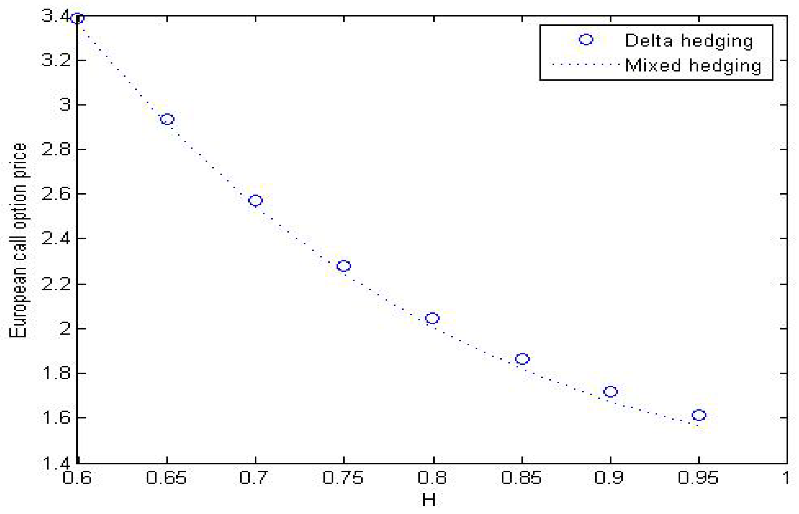
From Figure 1, we can see that the parameter H has an important influence on the European call option price. Moreover, as the parameter H increases, the difference in the European call option price between delta hedging and mixed hedging gradually becomes larger.

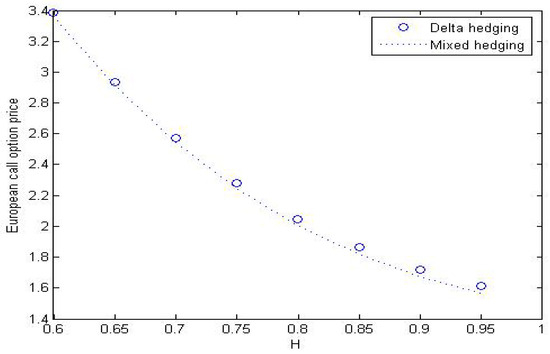
Figure 1. European call option price across Hurst parameter H.

4. Numerical Analysis

4.1. Price of European Call Option in Discrete Time under sfBm Model

In this subsection, we will compare the European call option price between delta hedging and mixed hedging. We set $S_0=49$, $r=0.05$, $T=1$, $\mu =0.11$, $\sigma =0.2$, $\Delta t=0.02$, $H=0.8$.

4.2. Comparison of Delta Hedging Method and Mixed Hedging Method in sfBm Model

In this subsection, we will compare the delta hedging and the mixed hedging strategies in the sfBm model across the hedging error ratio.

In order to compare the hedging error ratios of the two hedging methods, we use the same example as in [33] (i.e., example 3.1 of [33]). The values of the parameters are $S_0=49,K=50,\mu =0.11,\sigma =0.2,H=0.8$.

From Table 2, we can see that the European call option price under delta hedging at week 0 is $71,778.710. The discount of the total cost of writing the option and hedging to week 0 is equal to $106,355.902. The hedging error of delta hedging is $(106,355.902-71,778.710)/71,778.710$, which is close to $0.48172932$.

Table 2. Simulation of delta hedging per week with $T=20/52$ years.

Week	Stock Price	Delta	Shares Purchased	Cost of Shares Purchased	Cumulative Cost Including Interest	Interest Cost	Option Price
0	49	0.497333403	49,733.34	2,436,933.674	2,436,933.674	2343.205	0.717787102
1	49.45	0.584555406	8722.20	431,312.805	2,870,589.684	2760.182	0.917621068
2	50.32	0.750678897	16,612.35	835,933.407	3,709,283.273	3566.619	1.451814242
3	49.81	0.646630253	−10,404.864	−518,266.296	3,194,583.596	3071.715	1.044419038
4	50.86	0.834883451	18,825.320	957,455.765	4,155,111.076	3995.299	1.776745538
5	50.43	0.763181323	−7170.213	−361,593.832	3,797,512.543	3651.454	1.379749073
6	50.32	0.739377591	−2380.373	−119,780.379	3,681,383.618	3539.792	1.244182892
7	51.39	0.906823739	16,744.615	860,505.755	4,545,429.165	4370.605	2.080285620
8	51.54	0.925164351	1834.061	94,527.514	4,644,327.284	4465.699	2.164909300
9	50.65	0.802252336	−12,291.202	−622,549.356	4,026,243.627	3871.388	1.334854428
10	51.71	0.948091617	14,583.928	754,134.922	4,784,249.937	4600.240	2.219020546
11	52.04	0.972919347	2482.773	129,203.507	4,918,053.684	4728.898	2.484633325
12	52.60	0.992800929	1988.158	104,577.121	5,027,359.703	4834.000	2.986135035
13	53.83	0.999842305	704.138	37,903.727	5,070,097.43	4875.094	4.165455437
14	52.81	0.998258641	−158.366	−8363.330	5,066,609.194	4871.740	3.098185470
15	51.12	0.923907629	−7435.1012	−380,082.373	4,691,398.561	4510.960	1.393168349
16	50.71	0.857023251	−6688.438	−339,170.681	4,356,738.84	4189.172	0.9653540488
17	50.33	0.742755222	−11,426.803	−575,110.99	3,785,817.022	3640.209	0.5893340681
18	50.81	0.934088036	19,133.281	972,162.028	4,761,619.259	4578.480	0.9237137816
19	51.14	0.997258440	6317.0404	323,053.446	5,089,251.185	4893.511	1.188410772
20	52.07	1.000	274.156	14,275.303	5,108,419.999	4911.942	2.070000000

Hedging cost = $108,419.999, discounted hedging cost = $106,355.902, and hedging error ratio is 0.48172932.

From Table 3, we can see that the European call option price under mixed hedging is $69,141.684. The discount of the total cost of writing the option and hedging to week 0 is equal to $97,938.092. The hedging error of mixed hedging is $(97,938.092-69,141.684)/69,141.684$, which is approximately $0.41648404$. From Table 2 and Table 3, we can see that error ratio of mixed hedging is less than that of delta hedging.

Table 3. Simulation of mixed hedging per week with $T=20/52$ years.

Week	Stock Price	${\mathit{X}}_1(\mathit{t})$	Shares Purchased	Cost of Shares Purchased	Cumulative Cost Including Interest	Interest Cost	Option Price
0	49	0.519720461	51,972.046	2,546,630.254	2,546,630.254	2448.683	0.691416840
1	49.45	0.610171453	9045.0992	447,280.155	2,996,359.092	2881.115	0.892284217
2	50.32	0.777127706	16,695.625	840,123.865	3,839,364.072	3691.696	1.43154169
3	49.81	0.674473194	−10,265.451	−511,322.124	3,331,733.644	3203.590	1.02144752
4	50.86	0.858844664	18,437.147	937,713.296	4,272,650.530	4108.318	1.76175939
5	50.43	0.791102994	−6774.167	−341,621.242	3,935,137.606	3783.786	1.36173009
6	50.32	0.768722934	−2238.006	−112,616.462	3,826,304.930	3679.139	1.22587031
7	51.39	0.925707400	15,698.447	806,743.171	4,636,727.240	4458.392	2.07125983
8	51.54	0.942012829	1630.543	84,038.181	4,725,223.813	4543.484	2.15757677
9	50.65	0.831665364	−11,034.747	−558,909.910	4,170,857.387	4010.440	1.32094420
10	51.71	0.961938784	13,027.342	673,643.855	4,848,511.682	4662.030	2.21402296
11	52.04	0.981702680	1976.390	102,851.315	4,956,025.027	4765.409	2.48188050
12	52.60	0.995862606	1415.993	74,481.211	5,035,271.647	4841.607	2.98532983
13	53.83	0.999942406	407.98	21,961.563	5,062,704.817	4867.380	4.16543469
14	52.81	0.999200206	−74.22	−3919.558	5,063,652.639	4868.897	3.09799812
15	51.12	0.946413643	−5278.656	−269,844.910	4,798,676.626	4614.112	1.38841294
16	50.71	0.893540210	−5287.343	−268,121.179	4,535,169.559	4360.740	0.958587694
17	50.33	0.797629707	−9591.050	−482,717.562	4,056,812.737	3900.781	0.580916083
18	50.81	0.962372528	16,474.282	837,058.274	4,897,771.792	4709.396	0.921047903
19	51.14	0.999639073	3726.655	190,581.111	5,093,062.299	4897.175	1.18829746
20	52.07	1.000	36.093	1879.347	5,099,838.821	4903.691	2.070000000

Hedging cost = $99,838.821, discounted hedging cost = $97,938.092, and hedging error ratio is 0.41648404.

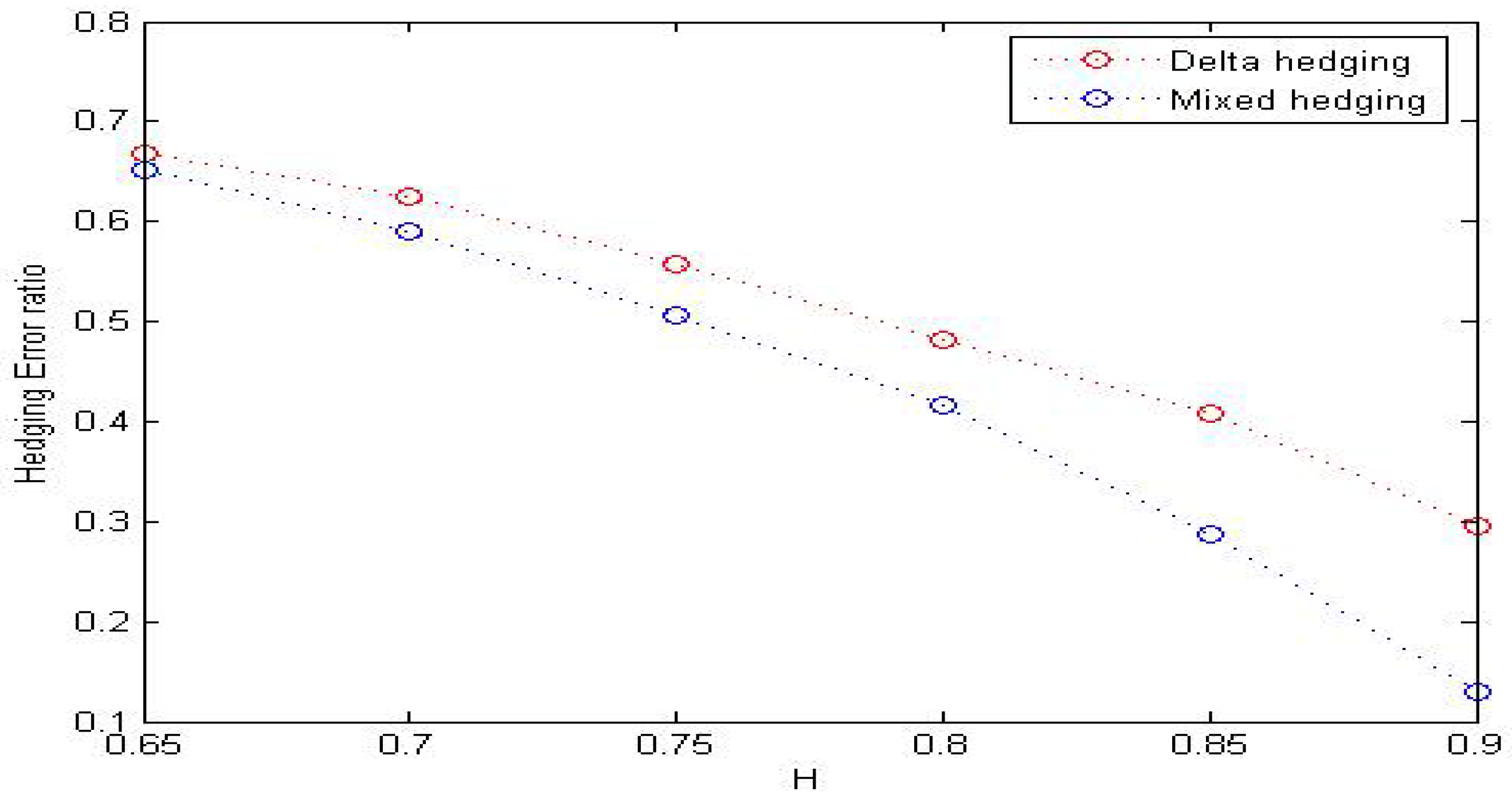
Table 4 and Figure 2 show the effects of Hurst parameter H on the hedging cost and hedging error ratio when H only varies from $0.65$ to $0.9$ $(S_0=49,K=50,\mu =0.11,$ $\sigma =0.2)$.

Table 4. Hedging error ratios under different Hurst parameters H.

H	Delta Hedging		Mixed Hedging
	Hedging Cost	Hedging Error Ratio	Hedging Cost	Hedging Error Ratio
0.65	122,108.260	0.66878962	116,423.210	0.65177851
0.7	118,896.608	0.62489765	112,041.758	0.58961575
0.75	113,917.756	0.55685429	106,155.329	0.50610081
0.8	108,419.999	0.48171932	99,838.821	0.41648404
0.85	103,072.969	0.40864427	90,728.643	0.28723150
0.9	94,729.545	0.29461906	79,601.134	0.12935765

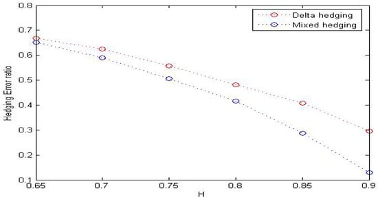
Figure 2. Hedging error ratio across Hurst parameter H.

From Table 4 and Figure 2, we can see that as Hurst parameter H increases, the hedging error ratios of the two hedging methods are both decreased, but the hedging error ratio of mixed hedging decreases faster.

5. Conclusions

This paper deals with the European call option pricing in discrete time under the sfBm model. The numerical results show that the European call option price of delta hedging is larger than the price of mixed hedging. The hedging error ratio of the mixed hedging strategy is less than that of the delta hedging strategy in some situations. Moreover, the Hurst parameter H plays an important role in the European call option price and hedging error ratio. Based on the results of this study, we can study option pricing under sfBm in discrete time; the future research directions mainly include the following.

(i) The real financial market is not smooth. The trading of the risk asset (like stock) always incurs transaction costs and dividends. Therefore, the study of the option pricing model with transaction costs or dividends in the sfBm regime is of great significance.

(ii) The changes in the risk asset price often accompany jumps. Both Brownian motion and sfBm cannot describe this situation. Thus, one can generalize the sfBm model to the jump-diffusion model in discrete time.

References

- Black, F.; Scholes, M.S. The pricing of options and corporate liabilities. J. Polit. Econ. 1973, 81, 637–659. [Google Scholar] [CrossRef]
- Necula, C. Option pricing in a fractional Brownian motion environment. Math. Rep. 2002, 2, 259–273. [Google Scholar] [CrossRef]
- Xiao, W.L.; Zhang, W.G.; Zhang, X.L.; Wang, Y.L. Pricing currency options in a fractional Brownian motion with jumps. Econ. Model. 2010, 27, 935–942. [Google Scholar] [CrossRef]
- Manley, B. How does real option value compare with Faustmann value when log prices follow fractional Brownian motion? Forest Policy Econ. 2017, 85, 76–84. [Google Scholar] [CrossRef]
- Wang, L.; Zhang, R.; Yang, L.; Su, Y.; Ma, F. Pricing geometric Asian rainbow options under fractional Brownian motion. Physica A 2018, 494, 8–16. [Google Scholar] [CrossRef]
- Yang, P.; Xu, Z.L. Numerical Valuation of European and American Options under Fractional Black-Scholes Model. Fractal Fract. 2022, 6, 143. [Google Scholar] [CrossRef]
- Dufera, T.T. Fractional Brownian motion in option pricing and dynamic delta hedging: Experimental simulations. N. Am. J. Econ. Financ. 2024, 69, 102017. [Google Scholar] [CrossRef]
- Nouty, C.E. The fractional mixed fractional Brownian motion. Stat. Probabil. Lett. 2003, 65, 111–120. [Google Scholar] [CrossRef]
- Sun, L. Pricing currency options in the mixed fractional Brownian motion. Physica A 2013, 392, 3441–3458. [Google Scholar] [CrossRef]
- Kim, K.H.; Yun, S.; Kim, N.U.; Ri, J.H. Pricing formula for European currency option and exchange option in a generalized jump mixed fractional Brownian motion with time-varying coefficients. Physica A 2019, 522, 215–231. [Google Scholar] [CrossRef]
- Chen, Q.S.; Zhang, Q.; Liu, C. The pricing and numerical analysis of lookback options for mixed fractional Brownian motion. Chaos Solitons Fractals 2019, 128, 123–128. [Google Scholar] [CrossRef]
- Xu, F.; Yang, X.J. Pricing European Options under a Fuzzy Mixed Weighted Fractional Brownian Motion Model with Jumps. Fractal Fract. 2023, 7, 859. [Google Scholar] [CrossRef]
- Magdziarz, M. Black scholes formula in subdiffusive regime. J. Stat. Phys. 2009, 136, 553–564. [Google Scholar] [CrossRef]
- Gu, H.; Liang, J.R.; Zhang, Y.X. Time-changed geometric fractional Brownian motion and option pricing with transaction costs. Physica A 2012, 391, 3971–3977. [Google Scholar] [CrossRef]
- Guo, Z.D. Option pricing under the Merton model of the short rate in subdiffusive Brownian motion regime. J. Stat. Comput. Sim. 2017, 87, 519–529. [Google Scholar] [CrossRef]
- Shokrollahi, F. The evaluation of geometric Asian power options under time changed mixed fractional Brownian motion. J. Comput. Appl. Math. 2018, 344, 716–724. [Google Scholar] [CrossRef]
- Corns, T.R.A.; Satchell, S.E. Skew Brownian Motion and Pricing European Options. Eur. J. Financ. 2007, 13, 523–544. [Google Scholar] [CrossRef]
- Zhu, S.P.; He, X.J. A new closed-form formula for pricing European options under a skew Brownian motion. Eur. J. Financ. 2018, 24, 1063–1074. [Google Scholar] [CrossRef]
- Pasricha, P.; He, X.J. Skew-Brownian motion and pricing European exchange options. Int. Rev. Financ. Anal. 2022, 82, 102120. [Google Scholar] [CrossRef]
- Hussain, S.; Arif, H.; Noorullah, M.; Pantelous, A. Pricing American Options under Azzalini Ito-McKean Skew Brownian Motions. Appl. Math. Comput. 2023, 451, 128040. [Google Scholar] [CrossRef]
- Song, S.Y.; Wang, X.C.; Zhang, X.W. Valuation of spread options under correlated skew Brownian motions. Eur. J. Financ. 2023, 2023, 2202821. [Google Scholar] [CrossRef]
- Bojdecki, T.; Gorostiza, L.G.; Talarczyk, A. Sub-fractional Brownian motion and its relation to occupation times. Stat. Probabil. Lett. 2004, 69, 405–419. [Google Scholar] [CrossRef]
- Tudor, C. Some properties of the sub-fractional Brownian motion. Stoch. Int. J. Probab. Stoch. Process. 2007, 79, 431–448. [Google Scholar] [CrossRef]
- Shen, G.J.; Chen, C. Stochastic integration with respect to the sub-fractional Brownian motion with H ∈ . Stat. Probabil. Lett. 2012, 82, 240–251. [Google Scholar] [CrossRef]
- Yan, L.; Shen, G.J.; He, K. Itô’s formula for a sub-fractional Brownian motion. Comm. Stoch. Anal. 2011, 5, 9. [Google Scholar]
- Nouty, C.E.; Zili, M. On the sub-mixed fractional Brownian motion. Appl. Math. Ser. B 2015, 30, 27–43. [Google Scholar]
- Rao, B.L.S.P. More on maximal inequalities for sub-fractional Brownian motion. Stoch. Anal. Appl. 2019, 38, 1686395. [Google Scholar]
- Araneda, A.A.; Bertschinger, N. The sub-fractional CEV model. Physica A 2021, 573, 125974. [Google Scholar] [CrossRef]
- Wang, W.; Cai, G.H.; Tao, X.X. Pricing geometric asian power options in the sub-fractional brownian motion environment. Chaos Solitons Fractals 2021, 145, 110754. [Google Scholar] [CrossRef]
- Wang, X.T.; Yang, Z.J.; Cao, P.Y.; Wang, S.L. The closed-form option pricing formulas under the sub-fractional Poisson volatility models. Chaos Solitons Fractals 2021, 148, 111012. [Google Scholar] [CrossRef]
- Bian, L.; Li, Z. Fuzzy simulation of European option pricing using sub-fractional Brownian motion. Chaos Solitons Fractals 2021, 153, 111442. [Google Scholar] [CrossRef]
- Xu, F.; Li, R.Z. The pricing formulas of compound option based on the sub-fractional Brownian motion model. J. Phys. Conf. Ser. 2018, 1053, 012027. [Google Scholar] [CrossRef]
- Wang, X.T.; Zhao, Z.F.; Fang, X.F. Option pricing and portfolio hedging under the mixed hedging strategy. Physica A 2015, 424, 194–206. [Google Scholar] [CrossRef]
- Kim, K.H.; Kim, S.H.; Jo, H.B. Option pricing under mixed hedging strategy in time-changed mixed fractional Brownian model. J. Comput. Appl. Math. 2022, 416, 114496. [Google Scholar] [CrossRef]
- Guo, Z.D.; Yuan, H.J. Pricing European option under the time-changed mixed. Physica A 2014, 406, 73–79. [Google Scholar] [CrossRef]
Disclaimer/Publisher’s Note: The statements, opinions and data contained in all publications are solely those of the individual author(s) and contributor(s) and not of MDPI and/or the editor(s). MDPI and/or the editor(s) disclaim responsibility for any injury to people or property resulting from any ideas, methods, instructions or products referred to in the content. |
© 2023 by the authors. Licensee MDPI, Basel, Switzerland. This article is an open access article distributed under the terms and conditions of the Creative Commons Attribution (CC BY) license (https://creativecommons.org/licenses/by/4.0/).