Abstract
In this paper, the inverse cumulative grey time power model with a Caputo fractional derivative is established, and the solution to the whitening equation is given by the Laplace transform. To improve the prediction accuracy of the model, the linear-tangent-function transformation is used to improve the smoothness of the data sequence, and a grey time power model is obtained, which has higher accuracy than the sinusoidal-function transformation, negative-exponential-function transformation and logarithmic-function transformation. The form and application range of the model are generalized.
1. Introduction
As the foundation and core content of grey theory, which was established by Professor Deng [1], the GM (1, 1) model has been applied to many systems and achieved remarkable results. However, both the prediction and fitting accuracy of the GM (1, 1) model are not high enough in practical applications, which greatly limits the application scope of the model. To extend and improve the GM (1, 1) model, many scholars have conducted a lot of improvement research and achieved good results. To reduce the error of the GM (1, 1) model, Zhu et al. [2] proposed a grey model with improved initial values, Cao et al. [3] proposed a grey model for optimizing background values, Li et al. [4] proposed a grey model for optimizing grey derivatives and Xie et al. [5] proposed the DGM model.
The grey prediction model with polynomials is one of the important improved models. It is established under the assumption that the data series conforms to the nonhomogeneous index trend. The time power model is taken as a special case. Xie et al. [6] constructed the NDGM model for approximating a nonhomogeneous exponential sequence. On this basis, Cui et al. [7] proposed the NGM (1, 1, k) model for a nonhomogeneous exponential sequence. Li et al. [8] proposed a grey seasonal model to predict the monthly natural gas production in China. Qian et al. [9] constructed a continuous time power model for the series with partial index features and discussed the model’s properties, applicable scope and time response. Wu et al. [10] solved the problem of optimal matching between the basic form of the time power model and the whitening equation. Ding et al. [11] solved the specific problem of solving the time–response function, which laid the foundation for the promotion and application of the model. Guo et al. [12] proposed an unequal interval time power model. Xie et al. [13] constructed a grey DGM (1, 1, N) model with time polynomials for an oscillation sequence. Wei et al. [14,15,16] studied the determination method of polynomial order in the GMP (1, 1, N) model with different methods.
Although the grey prediction model with time power can reflect the development trend of the real system better, it still has the following shortcomings. The model does not fully reflect the new-information-priority principle. Practical research has shown that the new-information-priority principle generated based on reverse accumulation could improve the prediction accuracy of the model [17,18]. The grey time power model based on integer order accumulation only has local memory and lacks overall memory. The fractional-order accumulation proposed by Wu [19] can compensate for the lack of overall memory better. Wu et al. [20] proved that the discrete grey model of the first-order cumulative generating operator violated the new-information-priority principle and minimum-information principle of the grey system theory and then proposed an NDGM model based on fractional-order accumulation. Zhou [21] constructed a fractional-order grey time power model based on repeatability for the prediction of hydropower consumption in China, and an example application showed that the model had better precision. Previous studies have shown that the smoothness of the raw data series affected the accuracy of the grey model to a certain extent, which greatly limited the application scope of the model [22,23,24]. Many scholars had studied the smoothness, stepwise ratio deviation, stepwise ratio variance, concave–convexity and reduction error of data sequences to improve the prediction accuracy of the grey model [25,26,27,28]. Finally, the continuous integer order derivatives were used to provide intermediate variables for the grey system, which damaged the prediction performance of the model. The memory principle of fractional derivatives could overcome these shortcomings [29,30,31].
To overcome the shortcomings, this paper proposes a time power model with a Caputo fractional derivative. The Laplace transform of the Mittag-Leffler function is used to solve the whitening equation. The method of fractional reverse-accumulation generation is used to solve the innovation priority and the overall memory. The ordinary least-squares method is used to estimate the model parameters. The hyperparameters are also estimated by establishing an optimization problem. Aiming at the fact that the smoothness of the original data series is low, this paper proposes linear-tangent-function transformation to improve the smoothness of the raw data and reduce the reduction error of the data transformation. The validity and practicability of the model are verified by forecasting the hydropower-consumption data of China. The model developed in this paper has important theoretical significance in enriching the theoretical modeling of the grey system and has important practical-application value in practice.
The rest of this paper proceeds as follows: The basic concepts and properties are introduced in Section 2. The grey time power model is constructed, and its properties and hyperparameters estimation are discussed in Section 3. The grey time power model based on linear-tangent-function transformation is established in Section 4. We take the hydropower-consumption data of China as an example to test the validity of the model in Section 5. The conclusion is discussed in Section 6.
2. Preliminaries
For the purposes of subsequent modeling, it is necessary to present some basics in this section. The first part of this section introduces the definition and some necessary properties of the Caputo fractional derivative and Laplace transform. The second part introduces the content of the grey time power model and sequence smoothness.
2.1. Caputo Fractional Derivative and Laplace Transform
Definition 1
as the inverse Laplace transform. Here, Re(s) is the real part of s.
([32]). Let ; the Laplace transform of the function is defined as
Name
Definition 2
([32]). The r-order Caputo fractional derivative is defined as
where is the Gamma function.
It can be seen from the above that the Caputo fractional derivative is an integral with parameters, and it is very difficult to calculate it directly. It needs to be processed first or by means of other function tools, such as the Laplace transform and Mittag-Leffler function.
Lemma 1
([32]). The Laplace transform of the r-order Caputo fractional derivative is represented as
Definition 3
([32]). The Multivariate Mittag-Leffler function is defined as
where
In particular, when , The Mittag-Leffler function of one variable is represented as
where and .
Lemma 2
([33]). The Laplace transform of the Mittag-Leffler function of one variable is defined as
where .
2.2. Grey Time Power Model and Sequence Smoothness
Definition 4.
Let be a raw data sequence, for and , equation
is defined as the grey time power model, abbreviated as the GM (r, 1, ) model, where and r and α are hyperparameters. is the r-order difference of . The parameter row ; here,
Obviously, when , it can be defined as the GM (r, 1, k) model. When , it is the GM (r, 1) model defined in reference [23].
Definition 5.
The whitening equation of the GM (r, 1, ) model is represented as
where is the Caputo fractional derivative.
Previous studies have shown that the smoothness of the data series has an important impact on the prediction and fitting accuracy of the model. Therefore, to improve the modeling accuracy, it is necessary to give a brief introduction to the concept and properties of sequence smoothness in this subsection.
Definition 6
([26,27]). Let be a non-negative original data series:
is called the smooth ratio of the sequence .
Lemma 3
([22]). is a smooth discrete data series if and only if the smooth ratio
is a monotone decreasing function of k.
Definition 7
([27,28]). Let be a non-negative original data series and name
as the stepwise ratio series of . So
is called the stepwise ratio series of after the function transformation.
Lemma 4.
Let be a non-negative raw data series; the non-negative data transformation can be written as , then
(I) Let be a monotone increasing data series, where is a strictly monotone decreasing function with x, and then .
(II) Let be a monotone decreasing data series, where is a strictly monotone increasing function with x, and then .
Proof.
Conclusion (I) is the result of Theorem 3 in reference [26] and Theorem 2 in reference [27]. The proof of conclusion (II) is like that of conclusion (I), which is omitted here. □
Lemma 5
([28]). Let the data transformation f be a differential function and satisfy , then the reduction error of the data transformation is unchanged or reduced.
3. The Construction of the Grey Time Power Model
In this section, the Laplace transform and Mittag-Leffler function are used to establish the grey time power model with a Caputo fractional derivative. To improve the prediction precision of the model and expand the application range of the model, the properties and the estimation of the hyperparameters of the model are discussed.
Theorem 1.
Let the accumulative order and power index ; the solution of the whitening equation for the GM (r, 1, ) model is
where is the indicative function of r.
Proof.
Let ; then . When , the Laplace transformation of Equation (1) is
According to Lemma 1 and , we obtain
then
take the inverse Laplace transform on two sides of the above equation, then
According to Lemma 2 and Definition 3, we gain that
According to the definition of a derivative, we have ; ignore and we obtain that , thus
When , in a similar method as above, we obtain
Combine (8) and (9), let and take , and Equation (2) is obtained. □
Grey time power model (2) contains two hyperparameters r and . According to different values of the hyperparameters, different properties can be obtained.
Property 1.
When and , the GM (r, 1, model degenerates to GM (r, 1), and the discrete form is
where .
Property 2.
When and , the GM (r, 1, model simplifies to GM (r, 1, k), and the discrete form is
Property 3.
When and , the GM (r, 1, model simplifies to GM (r,1,), and the discrete form is
In particular, when , Equation (10) is the result of reference [28]. When , Equation (10) is simplified to the GM (1, 1) model, Equation (11) is simplified to the GM (1, 1, k) model and Equation (12) is reduced to the GM (1, 1, ) model.
To improve the accuracy of the grey prediction model, the mean square error minimization is taken as the objective function to solve the hyperparameters:
where X and Y are given by Definition 4 and is the predicted value of term k.
4. Modeling Method and Process of GM (r, 1, ) Model after Data Transformation
Theorem 2.
If is a non-negative decreasing data sequence, then is a non-negative smooth data series.
Proof.
Because is a non-negative decreasing data series, for , and for , tangent function is strictly monotone increasing within , then ; thus, , so . □
Theorem 3.
If is a non-negative decreasing data sequence, then the data transformation can improve the stepwise ratio of the data sequence.
Proof.
Let ; for , function is strictly monotone and increasing in the interval . According to Lemma 4, conclusion (I), the result holds. □
Theorem 4.
The reduction error of the data transformation is reduced.
According to Lemma 5, the conclusion holds. Proof is omitted.
From all above, the tangent-function transformation can not only improve the smoothness but also reduce the reduction error.
Let be a non-negative original data series; the process of building a GM (r, 1, ) model based on a linear-tangent-function transformation is as follows:
Step 1. The non-negative decreasing data series is obtained, where usually takes .
Step 2. The data series is obtained.
Step 3. Based on the data sequence , the GM (1, 1, ) model is constructed and the prediction value is calculated.
Step 4. The prediction value of the original data series is obtained by the arctangent function and inverse linear-function transformation. The relative and average relative errors are also calculated.
5. Example Application
As a kind of renewable energy, water energy has the characteristics of low cost, small pollution and large reserves. It is an important guaranteed resource for China to realize the construction of ecological civilization and a sustainable-development strategy. As one of the main functions of hydropower, hydropower makes up a large proportion of the consumption structure of renewable resources in our country. At present, Chinese hydropower generation and installed capacity are ranked first in the world, but there is still a big gap between the economic development of hydropower and developed countries. Local water demand is the main basis for rational planning, dispatch and the allocation of water resources. Therefore, a reasonable and accurate hydropower forecast is of great significance to formulate a hydropower-development strategy in China [21]. Chinese hydropower-consumption data conform to the development trend from evolution, development to equilibrium, which is suitable for fitting and forecasting with the grey time power model.
The hydropower-consumption data of China from 2001 to 2018 are selected as the research object (data source: official website of National Bureau of Statistics of China). The original data from 2001 to 2015 are directly taken as the sample dataset, and the GM (r, 1, ) is established. The remaining data are used as the prediction dataset to test the fitting and prediction precision of the model. The parameters are given in Table 1.

Table 1.
Estimation result of parameters.
The GM (r, 1, ) prediction model (noted as GM (1.001, 1, )) based on the hydropower-consumption raw data of China is established as follows:
Equation (14) is used to predict Chinese hydropower-consumption data from 2001 to 2018. Both the average relative error of fitting (FARE) and average relative error of prediction (PARE) are calculated. The error results are compared with the different results in paper [21], as shown in Table 2.
Table 2.
Error comparison.
The error results indicate that the fitting precision of the GM (r, 1, ) model is 96.78%, which is higher than 95%. However, the prediction accuracy is 91.326%, which is lower than 95.142% of the RFGM (1, 1, ) model. The results show that the prediction accuracy of the model based on the original hydropower data is not high, and there is an overfitting phenomenon.
It is found that the smooth ratio is not a decreasing function of k. Therefore, the linear-function transformation is applied to the hydropower-consumption data from 2001 to 2018, and then the tangent-function transformation is also applied. The results are shown in Table 3.
Table 3.
Comparison of results.
It indicates that the data transformation can effectively improve the smoothness of hydropower-consumption data.
The GM (r, 1, ) model (noted as GM (0.999, 1, )) is established by using the first 15 items of the new series after linear-tangent-function transformation:
To test the effectiveness of the linear-tangent-function transformation, the logarithmic-function transformation [22], negative-exponential-function transformation [23] and sinusoidal-function transformation [24] are used to transform the hydropower-consumption data, and the first 15 items of the transformed data are used to construct the GM (r, 1, ) models.
The GM (r, 1, ) model (noted as GM (1.001, 1, )) based on the logarithmic-function transformation is as follows:
The GM (r, 1, ) model (noted as GM (0.981, 1, )) based on the sinusoidal-function transformation is as follows:
The GM (r, 1, ) model (noted as GM (0.896, 1, )) based on the negative-exponential-function transformation is as follows:
The predicted values of the Chinese hydropower-consumption data from 2001 to 2018 can be obtained by using the above four models, and the predicted values and average relative errors can be obtained by the corresponding inverse transform. The error results are given in Table 4.
Table 4.
Comparing errors under different transformations.
The errors of Chinese hydropower-consumption data based on four types of function transformation are discussed. The fitting accuracy of the logarithmic-function transformation is the highest, and the prediction precision is the worst. Compared with the GM (r, 1, ) model established directly with the original data, the fitting accuracy of the line-tangent-function transformation is the lowest, but the prediction accuracy is the highest. Figure 1 shows the boxplot of the fitting error.
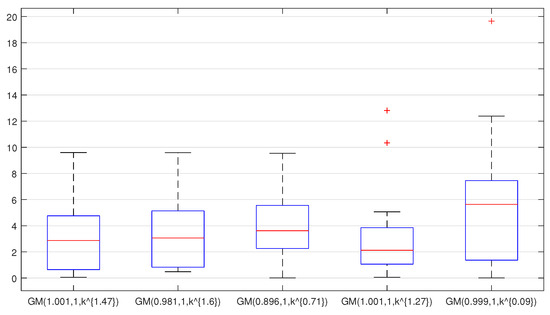
Figure 1.
Fitting error boxplot of different models.
The fitting precision of the GM (r, 1, ) model based on the sinusoidal-function transformation and the negative-exponential-function transformation is lower than that of the GM (r, 1, ) model based on the raw data, and the prediction precision of the models are not greatly improved. The overfitting phenomenon of the model is effectively solved. It indicates that the linear-tangent-function transformation method can effectively improve the smoothness of the Chinese hydropower-consumption data. The line chart of the models’ predictions is shown in Figure 2.

Figure 2.
Line chart of Chinese hydropower-consumption data forecast.
6. Conclusions
We propose a grey time power model with a Caputo fractional derivative. The grey forecasting models with primary or quadratic terms of time and the grey forecasting model without time terms are special cases of this paper. When the model is directly used to forecast Chinese hydropower-consumption data, there is a phenomenon of overfitting with a high fitting accuracy and insufficient prediction accuracy. In view of the low smoothness of Chinese hydropower-consumption data, the smoothness of the data is changed by using four kinds of function transformation. The grey prediction models with time power are established based on the new data series. The example application shows that the grey time power model with a Caputo fractional derivative based on a linear-tangent-function transformation has high prediction accuracy. It shows that the transformation of the linear-tangent function can effectively improve the smoothness of the hydropower-consumption data series. The time power model proposed in this paper is suitable for the prediction of Chinese hydropower-consumption data. For foreign hydropower-consumption data, as long as the data have partial exponential characteristics and partial linear characteristics, the model built in this paper is also suitable for forecasting such data.
Author Contributions
Conceptualization, P.H.; validation, C.-Y.G. and P.H.; formal analysis, P.H.; investigation, C.-Y.G. and P.H.; resources, C.-Y.G. and P.H.; writing—original draft, P.H.; writing—review and editing, C.-Y.G. and P.H.; visualization, P.H.; supervision, P.H.; project administration, C.-Y.G. All authors have read and agreed to the published version of the manuscript.
Funding
This research was funded by the Natural Science Foundation of Sichuan Province (no. 2023NSFSC0077) and the Natural Science Foundation of Xinjiang Uygur Autonomous Region of China (no. 2023D01A58).
Data Availability Statement
The original data of Chinese hydropower-consumption can be found on the official website of the National Bureau of Statistics of China; the other data are contained within the arcicle.
Conflicts of Interest
The authors declare no conflict of interest.
References
- Deng, J.L. Grey control system. J. Huazhong Inst. Technol. 1982, 3, 9–18. [Google Scholar]
- Zhu, X.Y.; Dang, Y.G.; Ding, S. Using a self-adaptive grey fractional weighted model to forecast Jiangsu’s electricity consumption in China. Energy 2020, 190, 116417. [Google Scholar] [CrossRef]
- Cao, Y.; Yin, K.D.; Li, X.M. Prediction of direct economic disasters based on the improved GM(1,1) model. J. Grey Syst. 2020, 32, 133–146. [Google Scholar]
- Li, B.; Wei, Y. Optimized grey derivative of GM(1,1). Syst. Eng. 2009, 29, 100–105. [Google Scholar]
- Xie, N.M.; Liu, S.F. Discrete grey forecasting model and its optimization. Appl. Math. Model. 2009, 33, 1173–1186. [Google Scholar] [CrossRef]
- Xie, N.M.; Liu, S.F.; Yang, Y.J.; Yuan, C.Q. On novel grey forecasting model based on non-homogeneous index sequence. Appl. Math. Model. 2013, 37, 5059–5068. [Google Scholar] [CrossRef]
- Cui, J.; Liu, S.F.; Zeng, B. A novel grey forecasting model and its optimization. Appl. Math. Model. 2013, 37, 4399–4406. [Google Scholar] [CrossRef]
- Li, N.; Wang, J.L.; Wu, L.F.; Bentley, Y. Predicting monthly natural gas production in China using a novel grey seasonal model with particle swarm optimization. Energy 2021, 215, 1191–1209. [Google Scholar] [CrossRef]
- Qian, W.Y.; Dang, Y.G.; Liu, S.F. Grey GM (1,1,tα) model with time power term and its application. Syst. Eng. Theory Pract. 2012, 32, 2247–2252. [Google Scholar]
- Wu, Z.H.; Wu, Z.C.; Li, F. Improved grey forecasting model with time power and its modeling mechanism. Control Decis. 2019, 34, 637–641. [Google Scholar]
- Ding, S.; Li, R.J.; Wu, S. Application of a novel structure-adaptative grey model with adjustable time power item for nuclear energy consumption foresting. Appl. Energy 2019, 34, 637–641. [Google Scholar]
- Guo, H.; Xiao, X.P.; Jeffrey, F. Non-equidistance GM (1,1,tα) model with time power and its application. Control Decis. 2015, 30, 1514–1518. [Google Scholar]
- Liu, S.F.; Zhu, C.Y.; Xie, N.M. On discrete grey system forecasting model corresponding with polynomial time-vary sequence. J. Grey Syst. 2013, 25, 1–18. [Google Scholar]
- Luo, D.; Wei, B.L. Grey forecasting model with polynomial term and its optimization. J. Syst. 2017, 29, 58–69. [Google Scholar]
- Wei, B.L.; Xie, N.M.; Hu, A.Q. Optimal solution for novel grey polynomial prediction model. Appl. Math. Model. 2018, 62, 717–727. [Google Scholar] [CrossRef]
- Wei, B.L.; Xie, N.M.; Yang, Y.J. Data-based structure selection for unified discrete grey prediction model. Expert Syst. Appl. 2019, 136, 264–275. [Google Scholar] [CrossRef]
- Shen, Q.Q.; Zhang, Z.J.; Qi, X.C.; Qiu, X.Y. Traffic flow prediction based on fractional seasonal grey model. J. Nantong Univ. Nat. Sci. Ed. 2021, 20, 37–42. [Google Scholar]
- Xu, Z.D.; Dang, Y.G.; Yang, D.L. Discrete grey forecasting model with fractional order polynomial and its application. Control Decis. 2023, 10, 1–7. [Google Scholar]
- Wu, L.F.; Liu, S.F.; Yao, L.G.; Xu, R.T. Using fractional order accumulation to reduce errors from inverse accumulated generating operator of grey model. Soft Comput. 2014, 19, 483–488. [Google Scholar] [CrossRef]
- Yao, T.X.; Wu, L.F.; Liu, S.F.; Cui, W. Non-homogeneous discrete grey model with fractional-order accumulation. Neural Comput. Appl. 2014, 25, 1215–1221. [Google Scholar]
- Zhou, W.J.; Cheng, Y.K.; Ding, S.; Dang, Y.G.; Wang, Z.X. Forecasting Chinese hydropower consumption forecasting by using the repeatability fractional grey time power model. Chin. J. Manag. Sci. 2023, 31, 279–286. [Google Scholar]
- Nie, Y.; Zhou, Y. The scenario research of land use change based on modified GM (1,1). Mathe Pract. Theory 2007, 37, 10–11. [Google Scholar]
- He, B.; Meng, Q. Study on generalization for grey forecasting model. Syst. Eng. Theory Pract. 2002, 9, 137–140. [Google Scholar]
- Cao, C.; Fan, C.J.; Hu, Z.G. Grey forecasting model and its application based on the sine function transformation. J. Math. (PRC) 2013, 33, 697–701. [Google Scholar]
- Zhang, J.; Ran, M.F. Grey modeling based on the transformation of Aarc cotx+B function. Grey Syst. Theory Appl. 2015, 5, 157–164. [Google Scholar] [CrossRef]
- Zhang, J.; Lü, X.; Ran M., F.; Han, G. DGM model based on Anti-cotangent function and its application. J. Grey Syst. 2016, 28, 63–74. [Google Scholar]
- Li, F.Q.; Liu, J.G. Research on data transformation for increasing accuracy of grey forecasting model. Stat. Decis. 2008, 20, 15–17. [Google Scholar]
- Qian, W.Y.; Dang, Y.G. New type of data transformation and its application in GM(1,1) model. Syst. Eng. Electr. 2019, 31, 2879–2881. [Google Scholar]
- Wu, L.F.; Liu, S.F.; Yao, L.G. Grey model with Caputo fractional derivative. Syst. Eng. Theory Pract. 2015, 35, 1311–1315. [Google Scholar]
- Mao, S.H.; Gao, M.Y.; Xiao, X.P.; Zhu, M. A novel fractional grey system model and its application. Appl. Math Model. 2016, 40, 5063–5076. [Google Scholar] [CrossRef]
- Xie, W.L.; Liu, C.X.; Li, W.D.; Wu, W.Z.; Liu, C. Continuous grey model with conformable fractional derivative. Chaos Solit. Fract. 2020, 139, 1–20. [Google Scholar] [CrossRef]
- Kilbas, A.; Srivastava, H.M.; Trujillo, J.J. Theory and Applications of Fractional Differential Equations, 1st ed.; Elsevier: Amsterdam, The Netherlands, 2006; pp. 1–132. [Google Scholar]
- Chen, W.; Sun, H.G.; Li, X.C. Fractional Derivative Modeling of Mechanical and Engineering Problems, 1st ed.; Science Press: Beijing, China, 2010; pp. 68–70. [Google Scholar]
Disclaimer/Publisher’s Note: The statements, opinions and data contained in all publications are solely those of the individual author(s) and contributor(s) and not of MDPI and/or the editor(s). MDPI and/or the editor(s) disclaim responsibility for any injury to people or property resulting from any ideas, methods, instructions or products referred to in the content. |
© 2023 by the authors. Licensee MDPI, Basel, Switzerland. This article is an open access article distributed under the terms and conditions of the Creative Commons Attribution (CC BY) license (https://creativecommons.org/licenses/by/4.0/).