Privacy Preservation of Nabla Discrete Fractional-Order Dynamic Systems

Abstract

This article investigates the differential privacy of the initial state for nabla discrete fractional-order dynamic systems. A novel differentially private Gaussian mechanism is developed which enhances the system’s security by injecting random noise into the output state. Since the existence of random noise gives rise to the difficulty of analyzing the nabla discrete fractional-order systems, to cope with this challenge, the observability of nabla discrete fractional-order systems is introduced, establishing a connection between observability and differential privacy of initial values. Based on it, the noise magnitude required for ensuring differential privacy is determined by utilizing the observability Gramian matrix of systems. Furthermore, an optimal Gaussian noise distribution that maximizes algorithmic performance while simultaneously ensuring differential privacy is formulated. Finally, a numerical simulation is provided to validate the effectiveness of the theoretical analysis.

1. Introduction

Fractional calculus is a generalization of classical calculus that extends derivatives and integrals from integer to non-integer orders. Due to their non-locality and hereditary properties, fractional calculus and fractional systems have drawn much attention and have been extensively studied in many fields, including signal processing [1], soft robots [2], medical science [3], economics [4], biology [5], and so on. Notably, its application in modeling various system dynamics and engineering scenarios demonstrates superior efficiency over traditional integer-order methods, particularly within the domain of control systems [6,7,8].

It is worth pointing out that most research on fractional-order systems has mainly focused on continuous-time models. However, with the rapid development of digital computers, discrete fractional calculus may play a more important role than its continuous-time counterparts in today’s digital era. As a result, there has been a growing interest in the study of discrete fractional calculus. For instance, the authors in [9] utilized the Grünwald–Letnikov definition and designed a finite-dimensional controller for discrete fractional-order systems with state disturbance. A modified Mikhailov stability criterion was presented to reduce the computational complexity for a class of non-commensurate discrete-time fractional-order systems in [10]. Recently, significant progress has been made in discrete fractional calculus based on the fractional sum and difference under various definitions [11,12,13] including the Riemann–Liouville and Caputo definitions, respectively. However, the aforementioned literature used delta fractional difference to describe discrete fractional-order systems. This approach limits the general applicability of the results by setting the initial state to zero and rendering the time series to rely on the order of the system. To overcome these limitations, the authors in [14] introduced nabla fractional differences and a discrete nabla analog of the Laplace transform. In [15], the fractional difference of Lyapunov inequalities and a stability analysis of nabla discrete fractional systems were developed. Furthermore, these results were extended to non-linear nabla fractional-order systems [16]. A discrete Mittag–Leffler stability was proposed in [17] to characterize the convergence rule for nabla discrete fractional-order systems and extend the Lyapunov directed method to discrete fractional systems under various definitions. In [18], the authors investigated the asymptotic stability of a non-linear nabla variable-order system. Furthermore, foundational mathematical properties such as the nabla Taylor series and Laplace transform for nabla tempered fractional calculus were explored in [19]. In control systems, the authors designed a discrete-time fractional-order proportional–integral–derivative (FOPID) controller in [20] using finite impulse response FIR filters and model order reduction methods. Additionally, the projective synchronization problem was investigated in [21] for nabla discrete fractional-order neural networks, according to the quaternion theory. By implementing a delay feedback controller, the quasi-uniform synchronization problem for discrete fractional fuzzy neural networks with mixed time delays was first discussed in [22]. The concepts of nabla fractional calculus and nabla fractional order systems have also been extensively studied, particularly in coordination control of multi-agent systems [23,24], as well as in distributed optimization problems [25]. The above research has made great contributions to the development of nabla discrete fractional-order systems, but they do not take into account the issue of privacy leakage within these systems.

Privacy preservation is a crucial aspect of information security, particularly for dynamic systems. In recent years, various methods have been developed for privacy protection, such as k-anonymity [26], l-diversity [27], and secure multiparty computation [28]. However, these approaches typically require a priori knowledge of the attackers’ background information, which may not be available in practice. To address this problem, differential privacy, a method introducing random noise into the data, has become a robust privacy-protection approach. For instance, the authors in [29] provided a comprehensive analysis of differential privacy techniques and demonstrated their application in three practical cases. Recently, differential privacy has been extensively studied in dynamic and cyber–physical systems. The concept of differential privacy was first introduced for dynamic systems in [30], and the authors discussed the Kalman filtering problem with differential privacy requirements. The average privacy-preserving consensus problem of multi-agent systems was investigated in [31], in which the differential privacy of initial values was taken into consideration. The authors in [32] developed a differentially private linear–quadratic control protocol for multi-agent systems and provided quantitative criteria for privacy preservation. Two differentially private gradient methods were proposed for distributed optimization problems in [33] to ensure both privacy and optimization accuracy. For some non-numerical or symbolic data, a novel differential privacy mechanism was proposed in [34] for protecting sensitive symbolic system trajectories and the results were applied to Markov chains. From the point of systems and control theory, the authors in [35] investigated the relation between differential privacy and strong input observability of the systems and designed a privacy-preserving controller for a tracking problem. Furthermore, by assuming that certain initial values are sensitive and the rest are public, a necessary and sufficient condition is established in [36] for preserving the differential privacy and unobservability of linear dynamical systems. However, it should be noted that these studies have primarily focused on integer-order systems where the issue of privacy preservation in nabla fractional-order dynamic systems has not been studied yet.

Inspired by the above discussion, this paper studies privacy protection in nabla discrete fractional-order dynamic systems via differential privacy. The main contributions of this paper are in three aspects:

• In contrast to the existing privacy-preserving literature that only concentrates on integer-order systems, this paper introduces a differential privacy mechanism for nabla discrete fractional-order dynamic systems. This method introduces Gaussian random noise into the output to prevent sensitive information from being inferred by malicious attackers.
• A connection between the differential privacy of initial values and the observability of nabla discrete fractional-order systems is provided. Furthermore, the paper proposes a sufficient condition for maintaining differential privacy via the observability Gramian matrix, effectively addressing the analytical challenges introduced by random noise in nabla fractional-order systems.
• An optimal Gaussian noise distribution is derived from an optimization problem. This distribution ensures the achievement of the desired privacy level while maintaining system performance.

The rest of this paper can be organized as follows: Section 2 introduces some notations and basic concepts of nabla fractional calculus. Section 3 formulates the problem statement for nabla discrete fractional systems. Section 4 analyzes the differential privacy for nabla fractional order systems. Section 5 presents a numerical example, and Section 6 concludes the paper.

2. Preliminaries

2.1. Notations

$\mathbb{N}$, $\mathbb{R}$ and $\mathbb{Z}\left({\mathbb{Z}}_{+}\right)$ denotes the natural number set, real number set, and integers (positive integers) set, respectively. For any $x_1,\dots ,x_m\in {\mathbb{R}}^n$, we denote $[x_1;\dots ;x_m]$ as a vector ${[x_1^T\dots x_m^T]}^T\in {\mathbb{R}}^{nm}$. For a vector $x\in {\mathbb{R}}^n$, denote ${\left|\right|x\left|\right|}_p$ as its p-norm. For a matrix $A\in {\mathbb{R}}^{n\times n}$, denote ${\left|\right|A\left|\right|}_2$ as its 2-norm, and its maximum and minimum eigenvalues are denoted by ${\lambda }_{max}\left(A\right)$ and ${\lambda }_{min}\left(A\right)$, respectively. Further, $A\succ 0$ means that A is symmetric and positive-definite. For any $a,b\in \mathbb{R}$, ${\mathbb{N}}_{a+1}=\{a+1,\dots ,\}$. For a random variable $\omega$, $\omega \sim {\mathcal{N}}_n(\mu ,\mathsf{\Sigma })$ means that $\omega$ has a non-degenerate multivariate Gaussian distribution with mean $\mu \in {\mathbb{R}}^n$ and covariance $\mathsf{\Sigma }\succ 0$, and its distribution has the following probability density:

$$p(\omega ;\mu ,\mathsf{\Sigma })={\left(\frac{1}{{\left(2\pi \right)}^{n}det\left(\mathsf{\Sigma }\right)}\right)}^{1/2}{e}^{{-|\omega -\mu |}^2{\mathsf{\Sigma }}^{-1}/2}.$$

The so-called Q-function is defined by $Q\left(\omega \right)=\frac{1}{\sqrt{2\pi }}{\int }_{\omega }^{\infty }{e}^{-\frac{v^2}{2}dv}$, where $Q\left(\omega \right)<1/2$ for $\omega >0$, and $R(ϵ,\delta )=(Q^{-1}\left(\delta \right)+\sqrt{{\left(Q^{-1}\left(\delta \right)\right)}^2+2ϵ})/2ϵ$.

2.2. Discrete Fractional Calculus

Some basic concepts and lemmas about discrete fractional calculus are presented.

Definition 1.

(Gamma function) For any $k\in \mathbb{R}\setminus \{\dots ,-2,-1,0\}$, the gamma function is defined by

$$\mathsf{\Gamma }\left(k\right)={\int }_0^{\infty }{e}^{-s}{s}^{k-1}ds.$$

(1)

Definition 2.

(Rising function) The rising function is defined by

$$t^{\overline{\alpha }}=\frac{\mathsf{\Gamma }(k+\alpha )}{k},k\in \mathbb{R}\setminus \{\dots ,-2,-1,0\}.$$

(2)

Definition 3.

For $f:{\mathbb{N}}_{a+1-n}\to \mathbb{R}$, its n-th integer-order backward difference is defined by

$${\nabla }^{n}f\left(k\right)=\sum _{i=0}^n{(-1)}^i\left(\genfrac{}{}{0pt}{}{n}{i}\right)f(k-i),k\in {\mathbb{N}}_{a+1},$$

(3)

where $n\in {\mathbb{Z}}_{+}$, ${\mathbb{N}}_{a+1}=\{a+1,a+2,\dots \}$, $a\in \mathbb{R}$ and $\left(\genfrac{}{}{0pt}{}{n}{i}\right)\triangleq \frac{\mathsf{\Gamma }(p+1)}{\mathsf{\Gamma }(q+1)\mathsf{\Gamma }(p-q+1)}$.

Definition 4.

For $f:{\mathbb{N}}_{a+1-n}\to \mathbb{R}$, its α-th sum with the Riemann–Liouville definition is defined as

$${}_a^R{\nabla }_k^{-\alpha }f\left(k\right)\triangleq \sum _{j=0}^{k-a-1}{(-1)}^j\left(\genfrac{}{}{0pt}{}{-\alpha }{j}\right)f(k-j),k\in {\mathbb{N}}_{a+1},$$

(4)

where $\alpha \in (n-1,n)$, $n\in {\mathbb{Z}}^{+}$, $a\in \mathbb{R}$.

Then, Equation (4) equals to the following expression

$$\begin{array}{cc}\hfill {}_a^R{\nabla }_k^{-\alpha }f\left(k\right)& =\sum _{j=0}^{k-a-1}\frac{{(j+1)}^{\overline{\alpha -1}}}{\mathsf{\Gamma }\left(\alpha \right)}f(k-j)\hfill \\ \hfill & =\sum _{j=a+1}^k\frac{{(k-j+1)}^{\overline{\alpha -1}}}{\mathsf{\Gamma }\left(\alpha \right)}f\left(j\right).\hfill \end{array}$$

(5)

Definition 5.

For $f:{\mathbb{N}}_{a+1-n}\to \mathbb{R}$, the nabla Riemann–Liouville and Caputo fractional differences are defined as

$${}_a^R{\nabla }_k^{\alpha }f\left(k\right){=}_a^R{\nabla }_k^{\alpha -n}{\nabla }^{n}f\left(k\right),k\in {\mathbb{N}}_{a+1},$$

(6)

$${}_a^C{\nabla }_k^{\alpha }f\left(k\right)={\nabla }^n{}_a^R{\nabla }_k^{\alpha -n}f\left(k\right),k\in {\mathbb{N}}_{a+1},$$

(7)

where $\alpha \in (n-1,n)$, $n\in {\mathbb{Z}}^{+}$, $a\in \mathbb{R}$.

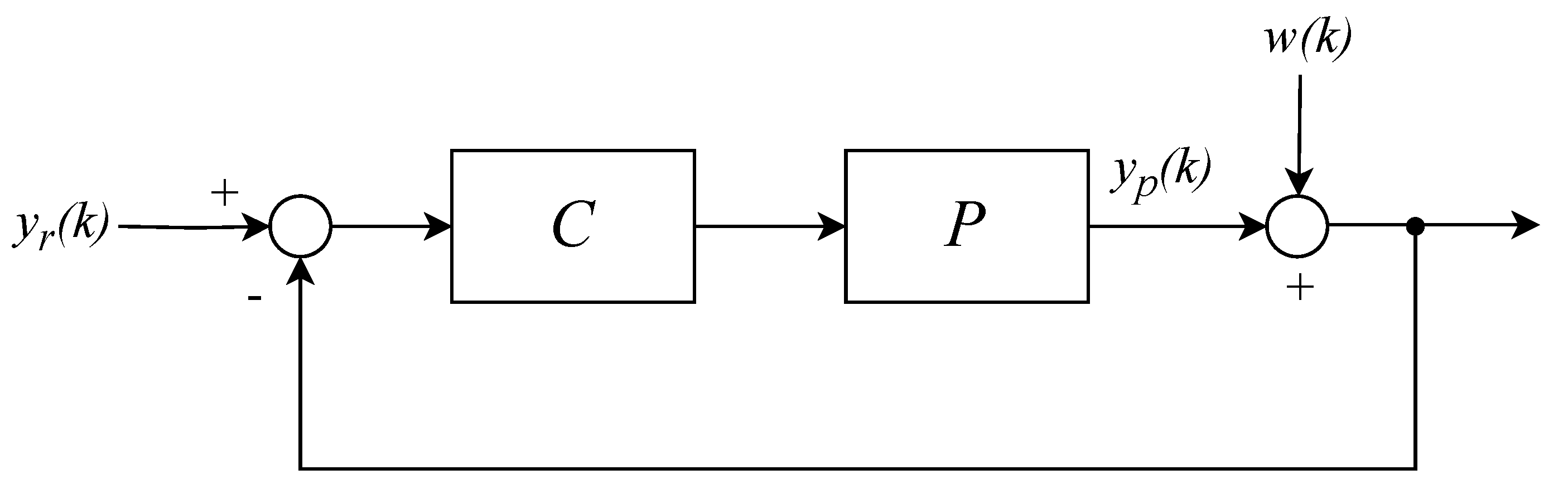
3. Problem Statement

Consider the following linear nabla discrete fractional-order systems with the Riemann–Liouville definition

$$\left\{\begin{array}{c}{}_0^R{\nabla }_k^{\alpha }x\left(k\right)=Ax\left(k\right)+Bu\left(k\right),k\in {\mathbb{N}}_1,\hfill \\ y\left(k\right)=Cx\left(k\right)+Du\left(k\right),\hfill \end{array}\right.$$

(8)

where $0<\alpha <1$, $y\left(k\right)\in {\mathbb{R}}^p$ is the output, and $u\left(k\right)\in {\mathbb{R}}^m$ is the input. $A\in {\mathbb{R}}^{n\times n}$, $B\in {\mathbb{R}}^{n\times m}$, $C\in {\mathbb{R}}^{p\times n}$, and $D\in {\mathbb{R}}^{p\times m}$ are the known constant matrices, respectively. In addition, $x\left(k\right)\in {\mathbb{R}}^n$ is the pseudo-state, which can be calculated using the following formula [14]

$$x\left(k\right)={\mathcal{F}}_{A,\alpha }\left(k\right)x_0+\sum _{s=1}^k{\mathcal{F}}_{A,\alpha }(k-s+1)Bu\left(s\right),$$

(9)

where $x\left(0\right)=x_0$ is the initial state and ${\mathcal{F}}_{A,\alpha }\left(k\right)={\sum }_{n=0}^k\frac{A^n{(k-n+1)}^{\overline{(n+1)\alpha -1}}}{\mathsf{\Gamma }\left(\right(n+1\left)\alpha \right)}$.

In this paper, we will focus on a finite dataset, which is consistent with studying the properties of a nabla dynamical system over a finite time. Given $y\left(0\right)$, $u\left(0\right)$, and a finite time $L\in {\mathbb{Z}}_{+}$, we denote the output sequence $Y_L:=[y\left(0\right);\dots ;y\left(L\right)]\in {\mathbb{R}}^{(L+1)p}$, and the input sequence $U_L:=[u\left(0\right);\dots ;u\left(L\right)]\in {\mathbb{R}}^{(L+1)m}$. Then, the output sequence $Y_L\in {\mathbb{R}}^{(L+1)p}$ of (8) can be written as

$$Y_L=O_L{x}_0+H_L{U}_L,$$

(10)

where $O_L\in {\mathbb{R}}^{(L+1)p\times n}$ and $H_L\in {\mathbb{R}}^{(L+1)p\times (L+1)m}$ are

$$O_L={\left[\begin{array}{ccccc}C& C\mathcal{F}\left(1\right)& C\mathcal{F}\left(2\right)& \dots & C\mathcal{F}\left(L\right)\end{array}\right]}^T,$$

(11)

$$H_L=\left[\begin{array}{ccccc}D& 0& \dots & \dots & 0\\ 0& C\mathcal{F}\left(1\right)B+D& \ddots & \ddots & ⋮\\ 0& C\mathcal{F}\left(2\right)B& C\mathcal{F}\left(1\right)B+D& \ddots & ⋮\\ ⋮& ⋮& \ddots & \ddots & 0\\ 0& C\mathcal{F}\left(L\right)B& C\mathcal{F}(L-1)B& \dots & C\mathcal{F}\left(1\right)B+D\end{array}\right],$$

(12)

$$\mathcal{F}\left(L\right)={\mathcal{F}}_{A,\alpha }\left(L\right)=\sum _{n=0}^L\frac{{(L-n+1)}^{\overline{\alpha n+\alpha -1}}}{\mathsf{\Gamma }(\alpha n+1)}{A}^n.$$

(13)

Throughout this paper, we consider the initial values $x\left(0\right)=x_0$ of system (8) to be privacy-sensitive.

4. Differential Privacy for Nabla Discrete Fractional-Order Systems

In this section, we study the differential privacy of nabla discrete fractional-order systems from three aspects. First, we analyze differential privacy based on a Gaussian mechanism that perturbs system outputs with random noise. Second, we give rank conditions for the observability of nabla discrete fractional-order systems and investigate the connection between observability and differential privacy. In particular, we characterize how the observability Gramian matrix impacts privacy guarantees. Finally, we formulate and solve an optimization problem to determine the minimum output noise quantity required to satisfy a specified level of differential privacy.

4.1. Differential Privacy with Output Noise

To prevent $x_0$ from being inferred from the published output data, random noise $w$ is added to the output such that $y_{w,k}=y\left(k\right)+w\left(k\right)$, and we denote the noise sequence $W_L:=[w\left(0\right);\dots ;w\left(L\right)]\in {\mathbb{R}}^{(L+1)p}$. Thus, the mapping $\mathcal{H}:{\mathbb{R}}^n\to {\mathbb{R}}^{(L+1)p}$ from the initial value $x_0$ to the output sequence $Y_{w,K}$ can be described as

$$Y_{w,L}=\mathcal{H}\left(x_0\right):=O_L{x}_0+H_L{U}_L+W_L.$$

(14)

Next, some definitions of differential privacy are given.

Definition 6.

Given $c>0$ and $r\in {\mathbb{Z}}_{+}$, a pair of input data $x_0,x_0^{{}^{\prime }}\in {\mathbb{R}}^n$ is said to be c-adjacent and is denoted by $Ad{j}_r^c$ if

$$\left|\right|x_0-x_0^{{}^{\prime }}{\left|\right|}_r\le c.$$

(15)

Then, we define the differential privacy of the mechanism (14).

Definition 7.

Given $ϵ>0$ and $\delta \ge 0$, the mechanism (14) is said to be $(ϵ,\delta )$ -differentially private at a finite time instant $L\in {\mathbb{Z}}_{+}$, if, for all $\mathcal{S}\subseteq range\left(\mathcal{H}\right)$,

$$\mathbb{P}[\mathcal{H}\left(x_0\right)\in \mathcal{S}]\le e^{ϵ}\mathbb{P}[\mathcal{H}\left(x_0^{{}^{\prime }}\right)\in \mathcal{S}]+\delta .$$

(16)

Theorem 1.

The mechanism (14) induced by $W_L\sim {\mathcal{N}}_{(L+1)p}(\mu ,{\mathsf{\Sigma }}_w)$ is $(ϵ,\delta )$ -differentially private at a finite time $L\in {\mathbb{Z}}_{+}$ for $Ad{j}_2^c$ with $ϵ>0$ and $0\le \delta \le 1$, if the covariance matrix ${\mathsf{\Sigma }}_w\succ 0$ is chosen such that

$${\lambda }_{max}^{-1/2}\left({\mathcal{O}}_{\mathsf{\Sigma },L}\right)\ge cR(ϵ,\delta ),$$

(17)

where ${\mathcal{O}}_{\mathsf{\Sigma },L}$ is defined by

$${\mathcal{O}}_{\mathsf{\Sigma },L}=O_L^T{\mathsf{\Sigma }}_w^{-1}{O}_L.$$

(18)

Proof. 

For any given $(x_0,x_0^{{}^{\prime }})\in Ad{j}_2^c$, define

$$p_L=(L+1)p,\zeta =Y_L-Y_L^{{}^{\prime }},Y_L=O_L{x}_0+H_L{U}_L,Y_L^{{}^{\prime }}=O_L{x}_0^{{}^{\prime }}+H_L{U}_L.$$

(19)

For any $ϵ>0$ and $\mathcal{S}\in \left({\mathbb{R}}^{p_L}\right)$, it follows that

$$\begin{array}{cc}\hfill & \mathbb{P}(Y_L+W_L\in \mathcal{S})={\int }_{{\mathbb{R}}^{p_L}}{\mathbb{1}}_{\mathcal{S}}(Y_L+w)p_{W_L}\left(w\right)dw\hfill \\ \hfill & ={\int }_{\mathcal{S}}{p}_{W_L}(z-Y_L^{{}^{\prime }}-\zeta )dz\hfill \\ \hfill & =\frac{1}{\sqrt{{\left(2\pi \right)}^{p_K}}det\left({\mathsf{\Sigma }}_w\right)}{\int }_{\mathcal{S}}exp\left(-\frac{\left|\right|z-Y_L^{{}^{\prime }}-\zeta {\left|\right|}_{{\mathsf{\Sigma }}_w^{-1}}^2}{2}\right)dz.\hfill \end{array}$$

(20)

Next, standard computation yields

$$\begin{array}{cc}\hfill & -\frac{\left|\right|z-Y_L^{{}^{\prime }}-\zeta {\left|\right|}_{{\mathsf{\Sigma }}_w^{-1}}^2}{2}\hfill \\ \hfill & =-\frac{\left|\right|z-Y_L^{{}^{\prime }}{\left|\right|}_{{\mathsf{\Sigma }}_w^{-1}}^2}{2}+\frac{2{(z-Y_L^{{}^{\prime }})}^T{\mathsf{\Sigma }}_w^{-1}\zeta -{\left|\right|\zeta \left|\right|}_{{\mathsf{\Sigma }}_w^{-1}}^2}{2}\hfill \\ \hfill & =ϵ-\frac{\left|\right|z-Y_L^{{}^{\prime }}{\left|\right|}_{{\mathsf{\Sigma }}_w^{-1}}^2}{2}+\frac{2{(z-Y_L^{{}^{\prime }})}^T{\mathsf{\Sigma }}_w^{-1}\zeta -{\left|\right|\zeta \left|\right|}_{{\mathsf{\Sigma }}_w^{-1}}^2-2ϵ}{2}.\hfill \end{array}$$

(21)

Inspired by these equalities, we divide $\mathcal{S}$ into $\mathcal{S}=(\mathcal{S}\setminus \tilde{\mathcal{S}}\left(\overline{a}\right))\cup \tilde{\mathcal{S}}\left(\overline{a}\right)$ with

$$\tilde{\mathcal{S}}\left(\overline{a}\right)=\{z\in S:2{(z-Y_L^{{}^{\prime }})}^T{\mathsf{\Sigma }}_w^{-1}\zeta -{\left|\right|\zeta \left|\right|}_{{\mathsf{\Sigma }}_w^{-1}}^2-2ϵ\ge 0\}.$$

(22)

We apply the following computation to the most right-hand side of (20)

$$\begin{array}{cc}\hfill & {\int }_{\mathcal{S}}exp\left(-\frac{\left|\right|z-Y_L^{{}^{\prime }}-\zeta {\left|\right|}_{{\mathsf{\Sigma }}_w^{-1}}^2}{2}\right)dz\hfill \\ \hfill & \le e^{ϵ}{\int }_{\mathcal{S}\setminus \tilde{\mathcal{S}}\left(\overline{a}\right)}exp\left(-\frac{\left|\right|z-Y_L^{{}^{\prime }}{\left|\right|}_{{\mathsf{\Sigma }}_w^{-1}}^2}{2}\right)dz+{\int }_{\tilde{\mathcal{S}}\left(\overline{a}\right)}exp\left(-\frac{\left|\right|z-Y_L^{{}^{\prime }}{\left|\right|}_{{\mathsf{\Sigma }}_w^{-1}}^2}{2}\right)\hfill \\ \hfill & \times \left(\frac{2{(z-Y_L^{{}^{\prime }})}^T{\mathsf{\Sigma }}_w^{-1}\zeta -{\left|\right|\zeta \left|\right|}_{{\mathsf{\Sigma }}_w^{-1}}^2}{2}\right)dz\hfill \\ \hfill & \le e^{ϵ}{\int }_{\mathcal{S}}exp\left(-\frac{\left|\right|z-Y_L^{{}^{\prime }}{\left|\right|}_{{\mathsf{\Sigma }}_w^{-1}}^2}{2}\right)dz+{\int }_{{\mathbb{R}}^{p_L}}exp\left(-\frac{\left|\right|z-Y_L{\left|\right|}_{{\mathsf{\Sigma }}_w^{-1}}^2}{2}\right){\mathbb{1}}_{\tilde{\mathcal{S}}\left(\overline{a}\right)}dz.\hfill \end{array}$$

(23)

From (16) we obtain, for any $ϵ>0,\mathcal{S}\in \mathcal{B}\left({\mathbb{R}}^{q_L}\right)$ ; thus, we have

$$\mathbb{P}(Y_L+W_L\in \mathcal{S})\le e^{ϵ}\mathbb{P}(Y_L^{{}^{\prime }}+W_L\in \mathcal{S})+\mathbb{P}\left(U\ge \frac{ϵ}{{\left|\right|\zeta \left|\right|}_{{\mathsf{\Sigma }}_w^{-1}}}-\frac{{\left|\right|\zeta \left|\right|}_{{\mathsf{\Sigma }}_w^{-1}}}{2}\right).$$

(24)

and $U\sim {\mathcal{N}}_1(0,1)$. Then, the mechanism is $(ϵ,\delta )-$ differential private if $Q(ϵ/|\left|\zeta \right|{|}_{{\mathsf{\Sigma }}_w^{-1}}-\left|\right|\zeta |{|}_{{\mathsf{\Sigma }}_w^{-1}}/2)\le \delta$, i.e.,

$${\left|\right|\zeta \left|\right|}_{{\mathsf{\Sigma }}_w^{-1}}^{-1}\ge R(ϵ,\delta ),$$

(25)

for any $(x_0,x_0^{{}^{\prime }})\in Ad{j}_2^c$. The inequality (25) holds if (17) is satisfied because

$${\left|\right|\zeta \left|\right|}_{{\mathsf{\Sigma }}_w^{-1}}=\left|\right|O_L(x_0-x_0^{{}^{\prime }}){\left|\right|}_{{\mathsf{\Sigma }}_w^{-1}}\le c{\lambda }_{max}^{1/2}\left({\mathcal{O}}_{\mathsf{\Sigma },L}\right).$$

(26)

From (18), ${\lambda }_{max}^{1/2}\left({\mathcal{O}}_{{\mathsf{\Sigma }}_w,L}\right)$ is the 2-induced matrix norm of ${\mathsf{\Sigma }}_w^{-1/2}{O}_L$, denoted by $\left|\right|{\mathsf{\Sigma }}_w^{-1/2}{O}_L{\left|\right|}_2$. This can be bounded as

$$\begin{array}{cc}\hfill {\lambda }_{max}^{1/2}\left({\mathcal{O}}_{{\mathsf{\Sigma }}_w,L}\right)& =\left|\right|{\mathsf{\Sigma }}_w^{-1/2}{O}_L\left|\right|\hfill \\ \hfill & \le \left|\right|{\mathsf{\Sigma }}_w{\left|\right|}_2\left|\right|O_L{\left|\right|}_2\hfill \\ \hfill & ={\lambda }_{min}^{-1/2}\left({\mathsf{\Sigma }}_w\right){\lambda }_{max}^{1/2}\left({\mathcal{O}}_{(L+1)q,L}\right).\hfill \end{array}$$

(27)

and consequently,

$${\lambda }_{max}^{-1/2}\left({\mathcal{O}}_{{\mathsf{\Sigma }}_w,L}\right)\ge {\lambda }_{min}^{1/2}\left({\mathsf{\Sigma }}_w\right){\lambda }_{max}^{-1/2}\left({\mathcal{O}}_{(L+1)q,L}\right).$$

(28)

Therefore, for any given $c,ϵ>0$ and $0<\delta <1/2$, one can make the Gaussian mechanism $(ϵ,\delta )$ -differentially private if one makes the minimum eigenvalue of the covariance matrix ${\mathsf{\Sigma }}_w$ sufficiently large such that

$${\lambda }_{min}^{1/2}\left({\mathsf{\Sigma }}_w\right)\ge c{\lambda }_{max}^{1/2}\left({\mathcal{O}}_{(L+1)q\mathrm{,}L}\right)R\left(ϵ\mathrm{,}\delta \right)\mathrm{.}$$

(29)

Then, together with (28) and (29), we can obtain (17). □

Remark 1.

In the special case with an independent and identically distributed(i.i.d.) Gaussian noise, where $\mathsf{\Sigma }={\sigma }^2{I}_{(L+1)q},\sigma >0$, (29) can be written as

$$\sigma \ge c{\lambda }_{max}^{1/2}\left({\mathcal{O}}_{(L+1)q,L}\right)R(ϵ,\delta ),$$

(30)

to make the mechanism $(ϵ,\delta )$ -differentially private.

4.2. Connection with Observability

It is evident that if the system (8) is observable, then the initial value $x_0$ can be determined from the output. This suggests an inherent relationship between the initial value exposure risk and the observability properties of linear nabla discrete fractional-order systems. Consequently, this subsection aims to further investigate the connection between observability and the protection of initial-value data via differential privacy.

First, we introduce the following definitions.

Definition 8.

The initial state $x_0$ of system (8) is said to be observable in a finite time $L\in {\mathbb{Z}}^{+}$ if it can be uniquely determined from the observation of output sequence $Y_L$. Otherwise, the system of (8) is said to be unobservable.

Definition 9.

The initial values $x_0$ are unobservable, if, for any pair of c-adjacent initial state $x_0,x_0^{{}^{\prime }}\in {\mathbb{R}}^n$, the following equation

$$\mathbb{P}[\mathcal{H}\left(x_0\right)\in \mathcal{S}]=\mathbb{P}[\mathcal{H}\left(x_0^{{}^{\prime }}\right)\in \mathcal{S}],$$

(31)

holds for all $\mathcal{S}\subseteq range\left(\mathcal{H}\right)$.

Next, we give some rank conditions of observability for linear nabla fractional-order systems.

Theorem 2.

The following statements are equivalent.

1 

The initial states $x_0$ of system (8) is observable in a finite time $L\in {\mathbb{Z}}_{+}$.

2 

The observability matrix $O_L$ has rank n.

3 

The observability Gramian matrix ${\mathcal{R}}_O\left(k\right)={\sum }_{s=1}^k{\mathcal{F}}_{A,\alpha }^T\left(s\right)C^{T}C{\mathcal{F}}_{A,\alpha }\left(s\right)$ has rank n.

Proof. 

(1)⇔(2)

(Sufficiency). According to Equation (9), we have

$$\begin{array}{cc}\hfill y\left(k\right)& =Cx\left(k\right)+Du\left(k\right)\hfill \\ \hfill & =C[{\mathcal{F}}_{A,\alpha }\left(k\right)x_0+\sum _{s=1}^k{\mathcal{F}}_{A,\alpha }(k-s+1)Bu\left(s\right)]+Du\left(k\right).\hfill \end{array}$$

(32)

Then, we have

$$\begin{array}{cc}\hfill C{\mathcal{F}}_{A,\alpha }\left(k\right)x_0& =y\left(k\right)-C\sum _{s=1}^k{\mathcal{F}}_{A,\alpha }(k-s+1)Bu\left(s\right)-Du\left(k\right)\hfill \\ \hfill & =\tilde{y}\left(k\right).\hfill \end{array}$$

(33)

According to (33), we have

$$\left[\begin{array}{c}C\\ C\mathcal{F}\left(1\right)\\ ⋮\\ C\mathcal{F}\left(L\right)\end{array}\right]x_0=\left[\begin{array}{c}\tilde{y}\left(0\right)\\ \tilde{y}\left(1\right)\\ ⋮\\ \tilde{y}\left(L\right)\end{array}\right].$$

(34)

Now, suppose $rank\left(O_L\right)=n$. Then, given $u\left(k\right)$ and a known $y\left(k\right)$, $x_0$ can be determined uniquely and $x_0\in {\mathbb{R}}^n$. This means the system (8) is observable.

(Necessity). Suppose the system is observable, then $x_0$ can be uniquely determined from the system of Equation (34). The system yields a unique solution for $x_0$, which means there exists at least n rows in $O_L$ that are linearly independent. Consequently, this implies that the rank of $O_L$ is n. The proof is complete.

(1)⇔(3)

(Sufficiency). Suppose the matrix ${\mathcal{R}}_O\left(k\right)$ has rank n. Multiplying both sides of (33) by ${\mathcal{F}}_{A,\alpha }^T\left(s\right)C^T$ and taking summation over the discrete time interval, we have

$$\begin{array}{cc}\hfill \sum _{s=1}^L{\mathcal{F}}_{A,\alpha }^T\left(s\right)C^{T}C{\mathcal{F}}_{A,\alpha }\left(s\right)x_0& =\sum _{s=1}^L{\mathcal{F}}_{A,\alpha }^T\left(s\right)C^T\tilde{y}\left(s\right)\hfill \\ \hfill {\mathcal{R}}_O\left(k\right)x_0& =\sum _{s=1}^L{\mathcal{F}}_{A,\alpha }^T\left(s\right)C^T\tilde{y}\left(s\right).\hfill \end{array}$$

(35)

Since rank $\left({\mathcal{R}}_O\left(k\right)\right)=n$, the matrix is invertible and

$$x_0={\mathcal{R}}_O{\left(k\right)}^{-1}\sum _{s=1}^L{\mathcal{F}}_{A,\alpha }^T\left(s\right)C^T\tilde{y}\left(s\right).$$

(36)

Thus, the system (8) is observable.

(Necessity). The contraction method is used in the proof. Suppose rank( ${\mathcal{R}}_O\left(k\right))<n$, then there exists a non-zero vector $\xi \in {\mathbb{R}}^n$ such that ${\mathcal{R}}_O\left(k\right)\xi =0$. Then, we obtain

$$0={\xi }^T{\mathcal{R}}_O\left(k\right)\xi =\sum _{s=1}^L\xi {\mathcal{F}}_{A,\alpha }^T\left(s\right)C^{T}C{\mathcal{F}}_{A,\alpha }\left(s\right)\xi =\sum _{s=1}^L\left|\right|C{\mathcal{F}}_{A,\alpha }\left(s\right)\xi {\left|\right|}_2^2,$$

(37)

which implies $C{\mathcal{F}}_{A,\alpha }\left(s\right)\xi =0$ for all $L>0$. Thus, $x\left(0\right)=x_0+\xi$ yields the same response for the system (8) as $x\left(0\right)=x_0$, which contradicts the assumption that the system (8) is completely observable. Therefore, $rank\left({\mathcal{R}}_O\left(k\right)\right)=n$. □

Then, we have the following theorems for differential privacy from the observability perspective.

Theorem 3.

Then, the mechanism (14) induced by $W_L\sim {\mathcal{N}}_{(L+1)p}(\mu ,{\mathsf{\Sigma }}_w)$ is $(ϵ,\delta )$ -differentially private at a finite time $L\in {\mathbb{Z}}_{+}$ for $Ad{j}_2^c$ with $ϵ>0$ and $0\le \delta \le 1$, if the covariance matrix ${\mathsf{\Sigma }}_w\succ 0$ is chosen such that

$${\lambda }_{min}^{1/2}\left({\mathsf{\Sigma }}_w\right)\ge c\left({\lambda }_{max}^{1/2}\left({\mathcal{R}}_O\left(k\right)\right)\right)R(ϵ,\delta ).$$

(38)

Proof. 

It holds that

$$\begin{array}{cc}\hfill & |O_L(x_0^{{}^{\prime }}-x_0){|}_{{\mathsf{\Sigma }}_w^{-1}}\hfill \\ \hfill & \le {\lambda }_{max}^{1/2}\left({\mathsf{\Sigma }}_w^{-1}\right)\left(\right|O_L(x_0^{{}^{\prime }}-x_0){|}_2)\hfill \\ \hfill & \le c{\lambda }_{max}^{1/2}\left({\mathsf{\Sigma }}_w^{-1}\right)\left({\lambda }_{max}^{1/2}\left({\mathcal{R}}_O\left(k\right)\right)\right).\hfill \end{array}$$

(39)

Since $1/{\lambda }_{max}\left({\mathsf{\Sigma }}_w^{-1}\right)={\lambda }_{min}\left(\mathsf{\Sigma }\right)$, from (25), we can obtain (38). □

Remark 2.

From (38), it can be inferred that the Gaussian mechanism’s differential privacy is defined by the maximum eigenvalue of the observability Gramian matrix. This implies that the less input observable system can be made highly differentially private with only a minimal amount of noise added.

Theorem 4.

The initial values $x_0$ of system (8) are unobservable if and only if

$$\mathrm{r}\mathrm{a}\mathrm{n}\mathrm{k}\left(O_L\right)<n\mathrm{.}$$

(40)

Proof. 

(Sufficiency). We suppose (40) holds. Thus, there exists non-zero vector $\rho \in ker\left(O_L\right)$ such that $O_L\rho =0$, then we obtain $O_L{x}_0=O_L(x_0+\rho )$, which, together with (31), implies

$$\mathbb{P}[\mathcal{H}\left(x_0\right)\in \mathcal{S}]=\mathbb{P}[\mathcal{H}(x_0+\rho )\in \mathcal{S}],$$

(41)

for all $\mathbb{H}\subseteq range\left(\mathcal{H}\right)$. Thus, this completes the proof by Definition 9.

(Necessity). To prove the necessity, we use the contraction method. With the unobservability of $x_0$, we suppose that (40) does not hold, i.e., $\mathrm{r}\mathrm{a}\mathrm{n}\mathrm{k}\left(O_L\right)=n$. Then, for all $x_0,x_0^{{}^{\prime }}$, we have $O_L(x_0-x_0^{{}^{\prime }})\ne 0$, yielding $O_L{x}_0\ne O_L{x}_0^{{}^{\prime }}$. Thus, from the definition of $\mathcal{H}$ in (10), it is clear that there exists $\mathbb{H}\subseteq range\left(\mathcal{H}\right)$ such that

$$\mathbb{P}[\mathcal{H}\left(x_0\right)\in \mathcal{S}]\ne \mathbb{P}[\mathcal{H}\left(x_0^{{}^{\prime }}\right)\in \mathcal{S}].$$

(42)

This contradicts the fact that the $x_0$ of the system (8) is unobservable. Therefore, it can be concluded that (40) holds, which completes the proof. □

Remark 3.

In terms of Definitions 7 and 9, a pair of $(x_0,x_0^{{}^{\prime }})$ that satisfies (31) would yield (16) with $ϵ=\delta =0$, implying perfect privacy. However, it cannot be conclusively said that the unobservability of $x_0$ directly infers its $(0,0)$ -differential privacy. Conversely, it is evident that for $ϵ=\delta =0$, the $(ϵ,\delta )$ -differential privacy of $x_0$ indeed implies its unobservability.

4.3. Minimization of the Noise

Building upon Equation (18), in this subsection, we determine the optimal Gaussian noise with the minimum energy that fulfills the sufficient condition (17) for differential privacy as established in Theorem 1. Specifically, we formulate an optimization problem wherein the covariance matrix of the Gaussian noise, denoted as ${\mathsf{\Sigma }}_w\succ 0$, is chosen as the decision variable.

Problem 1:

$$\begin{array}{cc}\hfill \underset{{\mathsf{\Sigma }}_w\succ 0}{\mathrm{minimize}}& Tr\left({\mathsf{\Sigma }}_w\right)\mathrm{,}\hfill \end{array}$$

(43)

$$\begin{array}{cc}\hfill \mathrm{subject}\mathrm{to}& {\lambda }_{max}\left(O_L^T{\mathsf{\Sigma }}_w^{-1}{O}_L\right)\le \frac{1}{c^2{R}^2\left(ϵ\mathrm{,}\delta \right)}\mathrm{.}\hfill \end{array}$$

(44)

Under certain specific assumptions and conditions, the solution to Problem 1 can be derived as follows:

Theorem 5.

Assume that $O_L$ is full rank, so the optimal solution to problem 1 is ${\mathsf{\Sigma }}_w^{*}=c^2{R}^2(ϵ,\delta )O_L{O}_L^T$.

Proof. 

Denote $\mathsf{\Phi }=cR(ϵ,\delta )O_L$, so that ${\mathsf{\Sigma }}_w^{*}=\mathsf{\Phi }{\mathsf{\Phi }}^T$. From (44), we have $I-{\mathsf{\Phi }}^T{\mathsf{\Sigma }}_w\mathsf{\Phi }⪰0$. According to the Schur complement, we have

$$\left[\begin{array}{cc}{\mathsf{\Sigma }}_w& \mathsf{\Phi }\\ {\mathsf{\Phi }}^T& I\end{array}\right]⪰0.$$

(45)

From (45), it implies that ${\mathsf{\Sigma }}_w⪰{\mathsf{\Sigma }}_w^{*}$. Consequently, for all ${\mathsf{\Sigma }}_w$ that satisfy the constraint, $Tr\left({\mathsf{\Sigma }}_w\right)\ge Tr\left({\mathsf{\Sigma }}_w^{*}\right)$. Therefore, we can find that ${\mathsf{\Sigma }}_w^{*}$ is the optimal solution with the minimal trace for Problem 1. □

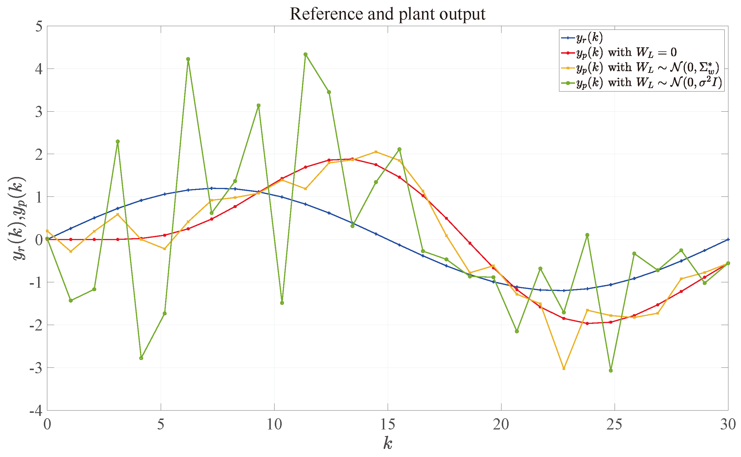
5. Numerical Example

In this section, a numerical example was provided to validate the effectiveness of the proposed algorithm.

Consider a feedback system in Figure 1, where the dynamic of plant P is given as

$$P:\left\{\begin{array}{cc}\hfill & {\nabla }_k^{\alpha }{x}_p\left(k\right)=A_p{x}_p\left(k\right)+B_p{u}_p\left(k\right),\hfill \\ \hfill & y_p\left(k\right)=C_p{x}_p\left(k\right),\hfill \end{array}\right.$$

(46)

where $x_p\in {\mathbb{R}}^{n_p}$, $u_p\in {\mathbb{R}}^{m_p}$, and $y_p\in {\mathbb{R}}^{q_p}$ are the state, input, and output, respectively, and $A_p$, $B_p$, $C_p$ are known matrices.

The dynamic of controller C is given as

$$C:\left\{\begin{array}{cc}\hfill & {\nabla }_k^{\alpha }{x}_c\left(k\right)=A_c{x}_c\left(k\right)+B_{c}e\left(k\right),\hfill \\ \hfill & u_p\left(k\right)=C_c{x}_c\left(k\right),\hfill \end{array}\right.$$

(47)

where $x_c\in {\mathbb{R}}^{n_c}$ is the state of the controller, $y_r\left(k\right)$ denotes the reference signal, and $e\left(k\right)=y_r\left(k\right)-y_p\left(k\right)$ is the tracking error signal. Then, the composite system consisting of the plant (46) and controller (47) is

$$\left\{\begin{array}{cc}\hfill & {\nabla }_k^{\alpha }\widehat{x}\left(k\right)=\widehat{A}\widehat{x}\left(k\right)+\widehat{B}{y}_r\left(k\right),\hfill \\ \hfill & y_p\left(k\right)=\widehat{C}\widehat{x}\left(k\right),\hfill \\ \hfill & e\left(k\right)=y_r\left(k\right)-\widehat{C}\widehat{x}\left(k\right),\hfill \end{array}\right.$$

(48)

where $\widehat{x}\left(k\right)=\left[\begin{array}{c}{x}_p\left(k\right)\\ x_c\left(k\right)\end{array}\right]$, $\widehat{A}=\left[\begin{array}{cc}{A}_p& B_p{C}_c\\ -B_c{C}_p& A_c\end{array}\right]$, $\widehat{B}=\left[\begin{array}{c}0\\ B_c\end{array}\right]$, $\widehat{C}=\left[\begin{array}{cc}{C}_p& 0\end{array}\right]$.

We assume that the attackers with access to the output $y_p\left(k\right)$ try to estimate the initial state of plant $x_p\left(0\right)$. The control objective is to minimize the tracking error $e\left(k\right)$ and preserve the privacy of the initial state of plant $x_p\left(0\right)$. In order to protect the sensitive information of $x_p\left(0\right)$, we consider adding output noise $w\left(k\right)$ to $y_p\left(k\right)$ such that $y_p\left(k\right)=\widehat{C}\widehat{x}\left(k\right)+w\left(k\right)$, and the feedback system with output noise is shown in Figure 1.

The dynamics of system (46) and (47) are given by $A_p=\left[\begin{array}{cc}1.2& -0.5\\ 1& 0\end{array}\right]$, $B_p={[-0.3,0]}^T$, $C_p=[0.2,0]$, $A_c=\left[\begin{array}{cc}1& 1\\ 0& 0.1\end{array}\right]$, $B_c={[0,-1]}^T$, $C_c=[1.5,0]$, and $\alpha =0.8$. We design the output noise to make the initial state of plant $x_p\left(0\right)$ differentially private for $L=30$, $c=2$, $ϵ=0.2$, and $\delta =0.1$, and the distribution of $W_L$ is given by $\mathcal{N}\sim (0,{\mathsf{\Sigma }}_w)$. We then obtain $R(ϵ,\delta )=0.2711$.

In what follows, we compare the following three cases (

Table 1. Comparison of different random noises.

Noise-Free	i.i.d. Noise	The Minimum Noise
$W_L=0$	$W_l\sim \mathcal{N}(0,{\sigma }_{i.i.d}^{2}I)$	$W_L\sim \mathcal{N}(0,{\mathsf{\Sigma }}_w^{*})$
$Tr\left({\mathsf{\Sigma }}_w\right)=0$	$Tr\left({\sigma }_{i.i.d}^{2}I\right)=34.545$	$Tr\left({\mathsf{\Sigma }}_w^{*}\right)=2.2784$

).

Figure 2 depicts the system output $y_p\left(k\right)$ and reference signal $y_r\left(k\right)$ for the three cases. The output error is the smallest in the noise-free case since the trajectory of $y_r\left(k\right)$ is fully utilized, increasing the potential for information leakage. In the case of i.i.d. noise, which has a uniform frequency distribution, there is an implication of an excessive out-of-band noise addition beyond the minimum required level. Consequently, this leads to a significant deterioration in tracking performance. In contrast, the optimized minimum noise strikes a balance, suppressing error fluctuations while preserving some tracking capability.

6. Conclusions

In this paper, we have studied a privacy-preserving problem of sensitive initial states for nabla discrete fractional-order dynamic systems. We developed a Gaussian mechanism by introducing output noise with $(ϵ,\delta )$ -differential privacy preserved. We analyzed the observability of nabla discrete fractional-order dynamic systems and derived its connection between differential initial-value privacy. Specifically, the differential privacy level of initial states can be characterized by the maximum eigenvalue of the observability Gramian matrix. Moreover, we formulated an optimization problem to derive the minimum energy random noise that satisfies the differential privacy requirement. In future works, the differential privacy approaches will be explored to develop a privacy-preserving controller for nabla fractional-order systems and the considered method will be utilized for nabla fractional-order multi-agent systems.

References

1. Yamni, M.; Daoui, A.; El Ogri, O.; Karmouni, H.; Sayyouri, M.; Qjidaa, H.; Flusser, J. Fractional Charlier moments for image reconstruction and image watermarking. Signal Process. 2020, 171, 107509. [Google Scholar] [CrossRef]
2. Wu, J.; Xu, Z.; Zhang, Y.; Su, C.Y.; Wang, Y. Modeling and tracking control of dielectric elastomer actuators based on fractional calculus. ISA Trans. 2023, 138, 687–695. [Google Scholar] [CrossRef] [PubMed]
3. Traver, J.E.; Nuevo-Gallardo, C.; Tejado, I.; Fernández-Portales, J.; Ortega-Morán, J.F.; Pagador, J.B.; Vinagre, B.M. Cardiovascular circulatory system and left carotid model: A fractional approach to disease modeling. Fractal Fract. 2022, 6, 64. [Google Scholar] [CrossRef]
4. Yousefpour, A.; Jahanshahi, H.; Munoz-Pacheco, J.M.; Bekiros, S.; Wei, Z. A fractional-order hyper-chaotic economic system with transient chaos. Chaos Solitons Fractals 2020, 130, 109400. [Google Scholar] [CrossRef]
5. Yin, Y.; Guo, J.; Peng, G.; Yu, X.; Kong, Y. Fractal operators and fractional dynamics with 1/2 order in Biological Systems. Fractal Fract. 2022, 6, 378. [Google Scholar] [CrossRef]
6. Chen, P.; Luo, Y.; Zheng, W.; Gao, Z.; Chen, Y. Fractional order active disturbance rejection control with the idea of cascaded fractional order integrator equivalence. ISA Trans. 2021, 114, 359–369. [Google Scholar] [CrossRef]
7. Belkhatir, Z.; Laleg-Kirati, T.M. High-order sliding mode observer for fractional commensurate linear systems with unknown input. Automatica 2017, 82, 209–217. [Google Scholar] [CrossRef]
8. Qi, F.; Qu, J.; Chai, Y.; Chen, L.; Lopes, A.M. Synchronization of incommensurate fractional-order chaotic systems based on linear feedback control. Fractal Fract. 2022, 6, 221. [Google Scholar] [CrossRef]
9. Alessandretti, A.; Pequito, S.; Pappas, G.J.; Aguiar, A.P. Finite-dimensional control of linear discrete-time fractional-order systems. Automatica 2020, 115, 108512. [Google Scholar] [CrossRef]
10. Stanisławski, R.; Latawiec, K.J. A modified Mikhailov stability criterion for a class of discrete-time noncommensurate fractional-order systems. Commun. Nonlinear Sci. Numer. Simul. 2021, 96, 105697. [Google Scholar] [CrossRef]
11. Baleanu, D.; Wu, G.C.; Bai, Y.R.; Chen, F.L. Stability analysis of Caputo–like discrete fractional systems. Commun. Nonlinear Sci. Numer. Simul. 2017, 48, 520–530. [Google Scholar] [CrossRef]
12. Wei, Y.; Su, N.; Zhao, L.; Cao, J. LMI based stability condition for delta fractional order system with sector approximation. Chaos Solitons Fractals 2023, 174, 113816. [Google Scholar] [CrossRef]
13. Zhu, Z.; Lu, J.G. LMI-based robust stability analysis of discrete-time fractional-order systems with interval uncertainties. IEEE Trans. Circuits Syst. I-Regul. Pap. 2021, 68, 1671–1680. [Google Scholar] [CrossRef]
14. Atici, F.M.; Eloe, P.W. Linear systems of fractional nabla difference equations. Rocky Mt. J. Math. 2011, 41, 353–370. [Google Scholar] [CrossRef]
15. Wei, Y.; Chen, Y.; Liu, T.; Wang, Y. Lyapunov functions for nabla discrete fractional order systems. ISA Trans. 2019, 88, 82–90. [Google Scholar] [CrossRef]
16. Wei, Y.; Zhao, L.; Wei, Y.; Cao, J. Lyapunov theorem for stability analysis of nonlinear nabla fractional order systems. Commun. Nonlinear Sci. Numer. Simul. 2023, 126, 107443. [Google Scholar] [CrossRef]
17. Wei, Y.; Wei, Y.; Chen, Y.; Wang, Y. Mittag–Leffler stability of nabla discrete fractional-order dynamic systems. Nonlinear Dyn. 2020, 101, 407–417. [Google Scholar] [CrossRef]
18. Hioual, A.; Ouannas, A.; Grassi, G.; Oussaeif, T.E. Nonlinear nabla variable-order fractional discrete systems: Asymptotic stability and application to neural networks. J. Comput. Appl. Math. 2023, 423, 114939. [Google Scholar] [CrossRef]
19. Wei, Y.; Zhao, L.; Zhao, X.; Cao, J. Enhancing the Mathematical Theory of Nabla Tempered Fractional Calculus: Several Useful Equations. Fractal Fract. 2023, 7, 330. [Google Scholar] [CrossRef]
20. Stanisławski, R.; Rydel, M.; Li, Z. A new reduced-order implementation of discrete-time fractional-order pid controller. IEEE Access 2022, 10, 17417–17429. [Google Scholar] [CrossRef]
21. Zhao, M.; Li, H.L.; Zhang, L.; Hu, C.; Jiang, H. Quasi-projective synchronization of discrete-time fractional-order quaternion-valued neural networks. J. Frankl. Inst. 2023, 360, 3263–3279. [Google Scholar] [CrossRef]
22. Gao, P.; Zhang, H.; Ye, R.; Stamova, I.; Cao, J. Quasi-uniform synchronization of fractional fuzzy discrete-time delayed neural networks via delayed feedback control design. Commun. Nonlinear Sci. Numer. Simul. 2023, 126, 107507. [Google Scholar] [CrossRef]
23. Ma, J.; Hu, J.; Zhao, Y.; Ghosh, B.K. Leader-Following Consensus Control of Nabla Discrete Fractional Order Multi-Agent Systems. IFAC-PapersOnLine 2020, 53, 2897–2902. [Google Scholar] [CrossRef]
24. Yuan, X.; Mo, L.; Yu, Y.; Ren, G. Containment control of fractional discrete-time multi-agent systems with nonconvex constraints. Appl. Math. Comput. 2021, 409, 126378. [Google Scholar] [CrossRef]
25. Hong, X.; Zeng, Y.; Zhou, S.; Wei, Y. Nabla fractional distributed optimization algorithm with directed communication topology. In Proceedings of the 2023 6th International Symposium on Autonomous Systems (ISAS), Nanjing, China, 23–25 June 2023; pp. 1–6. [Google Scholar]
26. Wang, J.; Cai, Z.; Yu, J. Achieving personalized k-anonymity-based content privacy for autonomous vehicles in CPS. IEEE Trans. Ind. Inform. 2019, 16, 4242–4251. [Google Scholar] [CrossRef]
27. Ashkouti, F.; Khamforoosh, K.; Sheikhahmadi, A. DI-Mondrian: Distributed improved Mondrian for satisfaction of the L-diversity privacy model using Apache Spark. Inf. Sci. 2021, 546, 1–24. [Google Scholar] [CrossRef]
28. Cramer, R.; Damgård, I.B.; Nielsen, J.B. Secure Multiparty Computation; Cambridge University Press: Cambridge, UK, 2015. [Google Scholar]
29. Dwork, C. Differential privacy: A survey of results. In Proceedings of the International Conference on Theory and Applications of Models of Computation, Xi’an, China, 25–29 April 2008; Springer: Berlin/Heidelberg, Germany, 2008; pp. 1–19. [Google Scholar]
30. Le Ny, J.; Pappas, G.J. Differentially private filtering. IEEE Trans. Automat. Contr. 2013, 59, 341–354. [Google Scholar] [CrossRef]
31. Liu, X.K.; Zhang, J.F.; Wang, J. Differentially private consensus algorithm for continuous-time heterogeneous multi-agent systems. Automatica 2020, 122, 109283. [Google Scholar] [CrossRef]
32. Yazdani, K.; Jones, A.; Leahy, K.; Hale, M. Differentially private LQ control. IEEE Trans. Automat. Contr. 2022, 68, 1061–1068. [Google Scholar] [CrossRef]
33. Wang, Y.; Nedić, A. Tailoring gradient methods for differentially-private distributed optimization. IEEE Trans. Automat. Contr. 2023, 1–16. [Google Scholar] [CrossRef]
34. Chen, B.; Leahy, K.; Jones, A.; Hale, M. Differential privacy for symbolic systems with application to Markov Chains. Automatica 2023, 152, 110908. [Google Scholar] [CrossRef]
35. Kawano, Y.; Cao, M. Design of privacy-preserving dynamic controllers. IEEE Trans. Automat. Contr. 2020, 65, 3863–3878. [Google Scholar] [CrossRef]
36. Wang, L.; Manchester, I.R.; Trumpf, J.; Shi, G. Differential initial-value privacy and observability of linear dynamical systems. Automatica 2023, 148, 110722. [Google Scholar] [CrossRef]
Figure 1. Feedback system with output noise.
Fractalfract 08 00046 g001
Figure 2. Reference signal y r ( k ) and plant output y p ( k ) under three random noises.
Fractalfract 08 00046 g002