Abstract
In engineering practice, the nonlinear vibration effect can easily lead to chaos in the system, which will not only reduce the performance of the system but also lead to premature fatigue of components, control failure, and increased safety risks. In view of the core position of the robotic arm in modern industry, this study relies on the robotic arm brake system to explore the theoretical basis of integrated viscoelastic materials as a vibration isolation layer. By analyzing the dynamic characteristics of the friction braking system with fractional differential terms, it aims to provide a new perspective for understanding and controlling the chaotic phenomena of a class of nonlinear friction systems. Firstly, we construct a model of a friction system and analyze its dynamic characteristics in detail. The self-excited vibration of the system under disturbance is studied. The relationship between amplitude and frequency is calculated by a nonlinear approximate analytical algorithm, and the accuracy of this relationship is verified by a numerical algorithm. Then, we compare the differences between non-fractional systems and fractional systems. It is found that with the increase in the fractional order term, the vibration amplitude of the system decreases significantly, which helps to reduce the nonlinear characteristics generated by the friction system and narrow the range of unstable solutions. Secondly, we also study the influence of parameter coefficients on the amplitude–frequency characteristics and analyze the local static bifurcation characteristics through singularity theory. Finally, we study the dynamic bifurcation behavior under different parameter perturbations and find that the change in system parameters will lead to the alternation of periodic motion and chaotic motion.
1. Introduction
In today’s society, collaborative robots [1] have become the fastest-growing and most widely marketed type in the global robot industry. The cooperation between collaborative robots and humans in industrial production can give full play to their respective advantages and improve work efficiency, thus forming a healthy and efficient production mode. Thus far, collaborative robots have been applied to various industries, such as manufacturing [2], automobiles [3], electronics [4], biomedicine [5], logistics [6], agriculture [7], aerospace [8], and many other industries. In the process of human–machine cooperation, we must first ensure the safety of both humans and machines. As an important component of robots, brakes can provide good protection for robots, especially when people manipulate machines, which can protect both the robot and the controller. Therefore, it is necessary to study brakes.
A brake is a device that slows down, stops, or maintains the stopped state of moving parts. It is widely used in high-speed rail [9], robotic arms [10], new energy electric vehicles [11], and other fields, attracting many scholars to study it. Yuan [12] used finite element software to compare the stability of brake systems with and without noise reduction pads, studying how the use of noise reduction pads improves brake friction squeal. Additionally, the relationship between the muffler’s structure and brake friction squeal was investigated. Liu et al. [13] conducted a study on the force amplification coefficient that affects the force transmission performance of the dry disk brake cartridge pressurization mechanism during the process and return stroke, aiming at the mobility and braking efficiency of tracked vehicles. Suo et al. [14] obtained the thermal elastoplastic constitutive relation of the brake disk through experiments and simulated the stress–strain response relationship of the lower brake disk using numerical calculations based on the sequential coupling method. In many countries, brakes are used to ensure the safety of joints and equipment, such as the robotic arm of the National Aeronautics and Space Administration [15], the European ERA [16], and the space robotic arm designed by Chinese universities [17].
Fractional calculus is an important branch of mathematics. Fractional calculus not only occupies an inevitable position in the development of mathematics, but its unique memory characteristics and precise description of real-world models, especially its simplicity in describing nonlinear models, have attracted widespread attention in both theory and practice. In response to the needs of applied disciplines, the theory and computational techniques of fractional calculus continue to advance and have become a core tool for solving complex scientific and engineering problems [18,19,20]. In some systems that require high accuracy, researchers have increasingly high requirements for describing systems. Applying fractional calculus to differential equations simplifies the resulting system differential equations, making the calculated results more accurate. Fractional calculus models are applied in various engineering fields [21,22,23,24,25,26,27,28]. To address the issue of low harmonic current at the DC bus in DC microgrid systems, Lin et al. [29] proposed a fractional capacitance-based method to force low harmonic currents. This method can theoretically achieve complete suppression of any or combination of low harmonic currents. Zhu et al. [30] used the backstepping method to design a boundary controller for fractional order reaction diffusion systems with spatially dependent coupling coefficients and proved the fitness of the observation gain and control gain kernel matrix equations. For error systems and closed-loop systems with output feedback, the Mittag–Leffler stability of the system was analyzed using the fractional order Lyapunov method. Moreover, using Wirtinger’s inequality, the stability conditions of the coupled system are improved, and a numerical solution method for the kernel function partial differential equation is given. Numerical simulation verifies the theoretical results. Zhu et al. [31] proposed fractional order power flow and voltage analysis for systems with fractional order inductors and capacitors. The results show that power system analysis based on fractional order component models can not only reduce reactive power losses in branches but also help improve voltage stability in power systems.
Viscoelastic materials [32] are widely used in various industries [33,34,35]. He et al. [36] used laminated piezoelectric actuators as active isolation elements and designed passive isolation elements based on viscoelastic materials. Li et al. [37] proposed a novel hybrid isolator for simulating rigid satellites. Tang et al. [38] studied rubber isolators for auxiliary power units. A nonlinear friction derivative dynamic model of rubber isolators has been established. Chang et al. [39] proposed a viscoelastic constitutive model for metal rubber that includes fractional order differentiation. Experimental results have shown that the proposed nonlinear dynamic system model of metal rubber with fractional order subterms has a continuous mathematical expression and can accurately reflect the complete dynamic performance of the nonlinear system of metal rubber.
In various projects, there are few linear problems but more nonlinear problems. Therefore, there have been many studies on nonlinear problems. Hamed [40] studied the approximate nonlinear dynamic behavior of AFM systems using perturbation methods and frequency response analysis. Kandil et al. [41] studied the oscillation behavior of the bearing system and derived a nonlinear dynamic equation for the control system. In order to eliminate the vibration of nonlinear dynamic beams, Ms et al. [42] added active control to their research and analyzed its stability, obtaining analytical and numerical solutions. Wang [43,44] established a nonlinear dynamic equation for the relative rotation system of two end-face rotating shafts, qualitatively analyzed the dynamic equation of equal torque, and studied the stability and other properties of the equation. Finally, an approximate analytical algorithm was developed to calculate the approximate solution of the equation under specific conditions. In addition, the uniqueness and exact periodic solutions of a class of relative rotational nonlinear dynamic systems were also studied.
In summary, the research on robots and brakes mainly considers the design of robot brakes and the dynamic performance of disk brakes. However, the dynamic performance analysis of nonlinear systems in robot electromagnetic brakes that incorporate fractional differentiation has not yet been fully investigated. In this paper, viscoelastic materials are added to the electromagnetic brake of a robot, which is used as a vibration isolation layer. The stress of the newly added material is represented by a fractional order term, thereby establishing a dynamic model of the electromagnetic brake of a robotic arm with fractional differentiation. We calculated the relationship between the frequency and amplitude under perturbation external conditions. By altering the external conditions, this study examined the characteristics of the friction system, analyzed the conditions for bifurcation behavior, and analyzed the local static and global steady-state characteristics.
2. Calculating an Approximate Solution
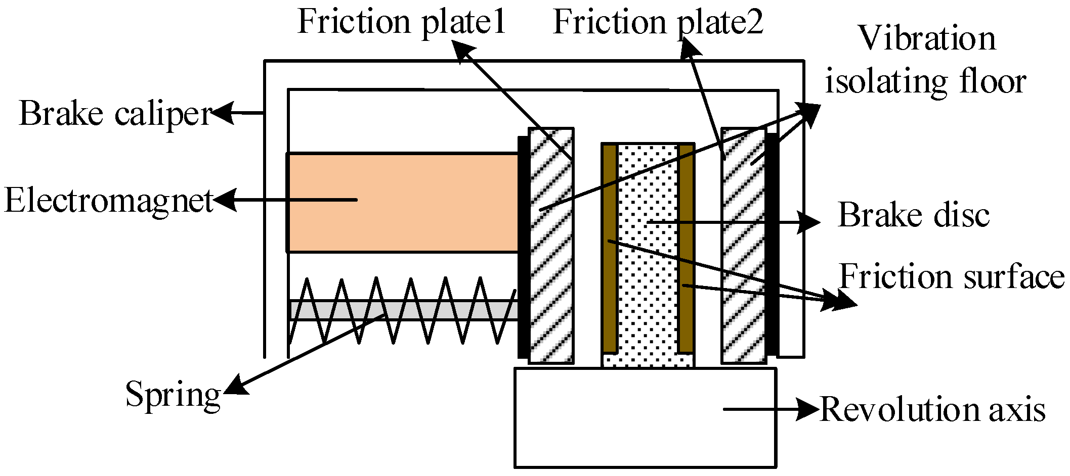
The new brake of the robotic arm is composed of a friction plate, brake caliper, electromagnet, spring, brake disk, shaft, and vibration isolation layer. Figure 1 is the functional structure diagram of the new electromagnetic brake of the robotic arm with vibration isolation layer. Figure 2 shows two states of the electromagnetic brake: (a) When the electrical current is switched off, the friction plate contacts the brake disk under the action of spring force, and the torque generated by the system is quickly stopped by the drive shaft. (b) When the current passes through the magnetic coil of the electromagnetic brake, the friction plate is pulled apart under the action of the magnetic force, releasing the brake disk. At this time, the transmission shaft runs normally.

Figure 1.
Functional structure diagram of new electromagnetic brake for robotic arm with vibration isolation layer.
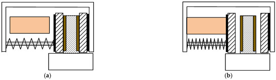
Figure 2.
Different states of the new electromagnetic brake of the robotic arm. (a) Electromagnet power-off braking state. (b) Electromagnet power-on starting state.
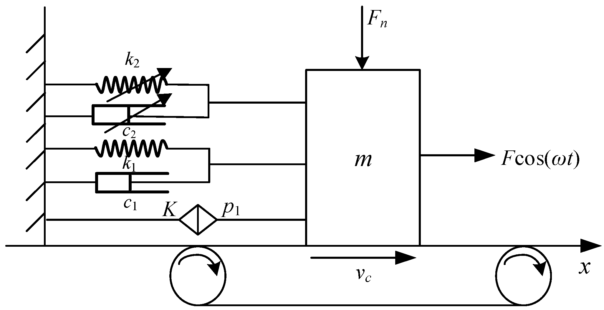
By analyzing the braking process of the electromagnetic brake, obtain the simplified model (Figure 3):

Figure 3.
Nonlinear dynamic model of the new electromagnetic brake of a robotic arm.
Kinetic equation:
In Equation (1), k1 and k2 are linear and nonlinear stiffness coefficients; c1 and c2 are linear and nonlinear damping coefficients, respectively; is defined as an external disturbance function; is the fractional derivative; () is the order of the fractional derivative; and K(K > 0) is the coefficient of the fractional derivative. is the friction between the mass and the conveyor belt, which belongs to dry friction.
There are many forms of definitions of fractional differential. In this paper, the expression of fractional order terms is defined using the Caputo [45] definition. Let the domain of the function x(t) be (a, b), and assume that x(t) is continuously differentiable up to order n on (a, b), where n − 1 < p < n and p > 0, then the Caputo fractional derivative is defined as follows:
In Equation (2), is a Gamma function satisfying when z > 0.
In order to study the vibration generated by the brake during braking and its impact on frictional vibration, a static friction model is applied to the motion process of the system as a friction force. For high-performance motion control, in addition to the robot’s own coupling and nonlinear time-varying effects, the effect of nonlinear friction, such as the Stribeck effect, is particularly pronounced at low speeds. The dry friction model with the Stribeck effect exhibits a negative slope characteristic at low relative velocities. When the relative velocity reaches a certain threshold, the dry friction coefficient remains unchanged. In this paper, a dry friction model with the Stribeck effect is selected.
where denotes external force and expresses the negative slope characteristics of the friction coefficient using a polynomial function model:
where represents the coefficient of friction; k3 and k4 are constants; is the maximum static friction coefficient; and vc is the speed of the conveyor belt.
In actual robotic arm operation, the brake usually works in a state close to equilibrium, and the nonlinear effect of its dynamic response is relatively weak. Introducing a small parameter can simulate this weak nonlinear effect, making the model closer to actual operating conditions. Therefore, Equation (1) is simplified into the following dimensionless form:
where , , , , , , , , , , , and .
This article uses the average method to obtain the analytical solution of the system. The averaging method is a technique for handling weakly nonlinear system dynamics, which simplifies problem solving by separating the fast oscillations and slow varying parts of the system response and eliminating the fast oscillations. This method transforms complex nonlinear problems into easier-to-handle linear or weakly nonlinear problems, preserving key dynamic characteristics of the system and helping to predict long-term behavior. In this article, the average method can effectively analyze the dynamic behavior of the robotic arm brake and provide theoretical support for design optimization. Let and be tuning factors, then Equation (5) can be written as follows:
When , the solution of the derived system and its derivative are as follows:
The changes of and are considered here. Let , by differentiating Equation (8) to time t and eliminating Equation (9), we obtain the following:
Further obtaining:
where:
Integrate Equations (12) and (13) as follows:
Before calculating the fractional integral, it is important to introduce two basic formulas:
Using the residue theorem and the contour integral:
Calculate the integral of the first part of Equation (15):
Similarly, it can be determined that when , in Equation (21) approaches 0, so:
Using the same method, we can obtain the integral of the first part of Equation (16).
Next:
Finally:
Therefore, it is obtained that:
The singular point in the moving phase plane is the solution of Equations (29) and (30), and eliminating leads to the amplitude frequency curve equation of the nonlinear system:
3. Stability Analysis
Analyze the stability of the system. Let and to obtain:
Let , , and substitute Equations (32) and (33):
where .
The characteristic determinant can be obtained from Equations (34) and (35) as follows:
where λ is the root of the characteristic equation,
According to the Lyapunov stability theory and Routh criterion, if N1 > 0 and N2 > 0, the trajectory of the singularity is asymptotically stable. If N2 < 0, the trajectory corresponding to the singularity is unstable. Therefore, N2 = 0 is the critical condition for determining whether the trajectory is stable.
4. Curve of Amplitude Versus Frequency and Verification of Numerical Solution
According to Equation (31), take a set of operating conditions as follows: F0 = 1, Fn = 0.2, m = 1, k1 = 1, k2 = 1, k3 = 1, k4 = 0.1, c1 = 0.1, c2 = 0.01, K = 0.8, p = 0.4, vc = 0.1, and us = 0.1.
Analyze the relationship between the amplitude and frequency of a system with fractional subdivisions (FOS, K = 0.8, p = 0.4) and a system without fractional subdivisions (NFOS, K = 0, p = 0).
Obtained from Figure 4, the amplitude–frequency relationship curve lags behind, and there are unstable regions in both FOS and NFOS. In FOS, it can be seen that due to the existence of fractional subdivisions, the maximum value of the curve is reduced, and the nonlinearity is also reduced. The figure shows that with A as the demarcation point, when the abscissa , the amplitude of FOS is greater than that of NFOS, and when the abscissa , the amplitude of FOS is less than that of NFOS.
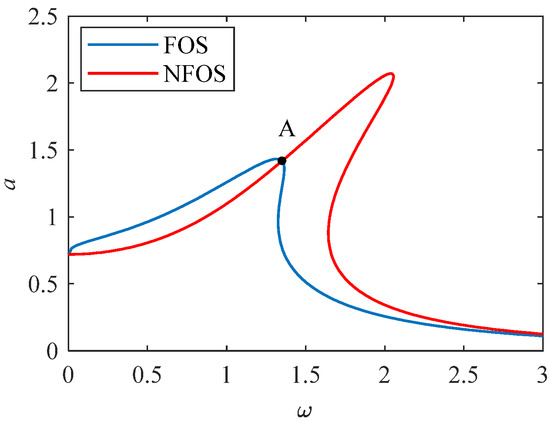
Figure 4.
System amplitude–frequency response curve.
Using the Runge–Kutta numerical method to verify the accuracy of the approximate analytical solution for the main resonance of the system calculated by the averaging method. Calculate the numerical iteration format of the system:
where is displacement; is velocity; is fractional order sub-item; and h is step size.
The numerical solution of the system was obtained by forward and backward frequency scanning, as shown in Figure 5. Comparing the approximate analytical solution calculated by the averaging method with the solution calculated by the numerical method, it was found that the solutions obtained by the two methods were relatively close, and the correctness of the approximate analytical solution could be obtained.
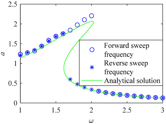
Figure 5.
Comparison diagram of analytical and numerical solutions.
5. Analysis of Amplitude Frequency Response Characteristics
Analyze the amplitude–frequency response characteristics under different parameter values. The obtained results are represented in Figure 6, Figure 7, Figure 8, Figure 9, Figure 10, Figure 11, Figure 12, Figure 13, Figure 14 and Figure 15.
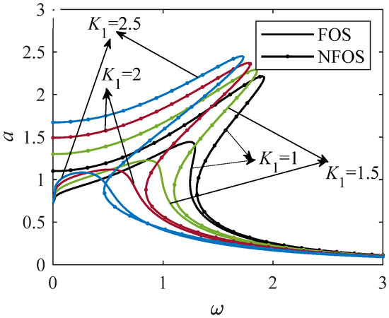
Figure 6.
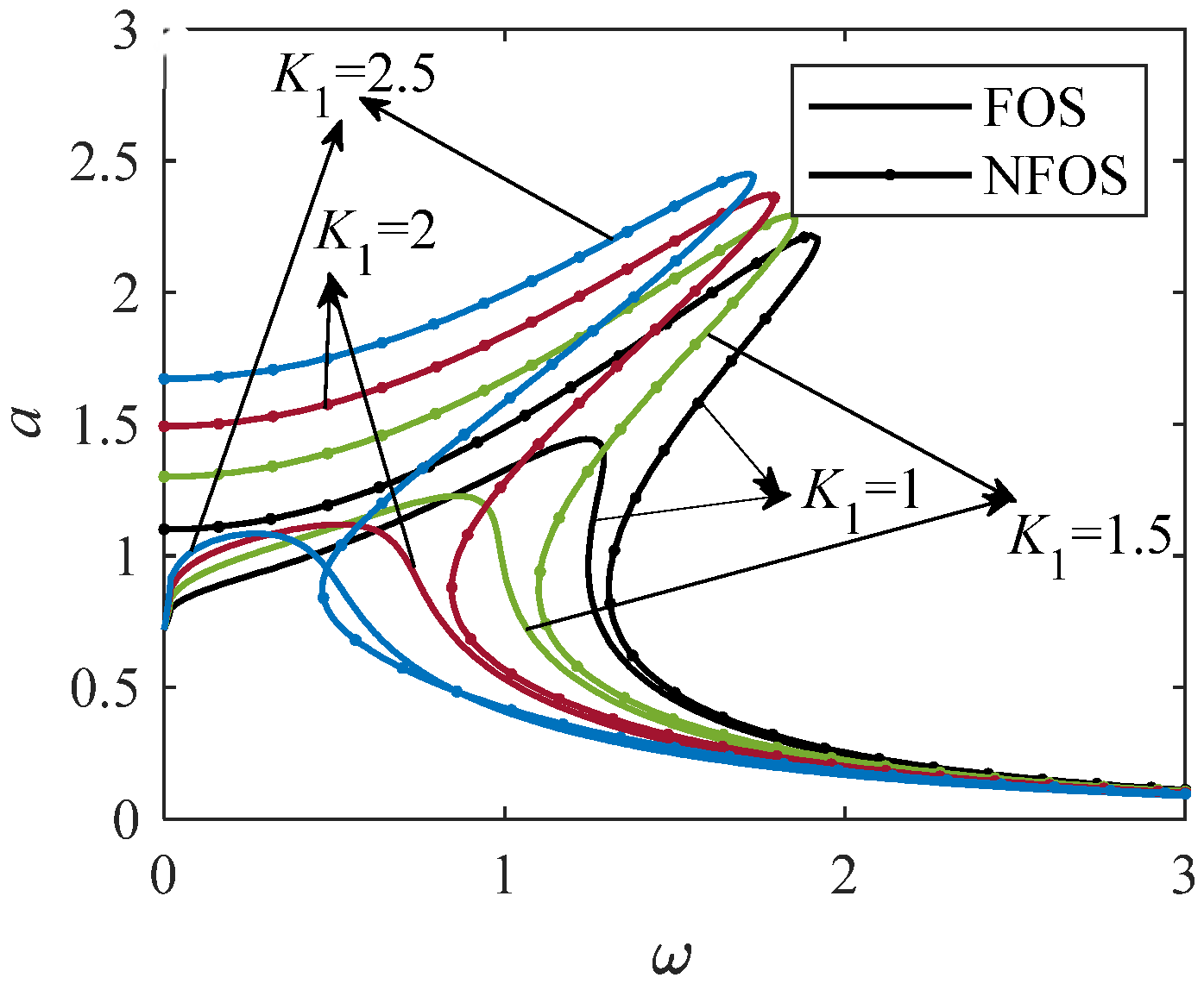
The effect of K pairs on the amplitude and frequency relation curves of FOS (p = 0.33) and NFOS (p = 0).

Figure 7.
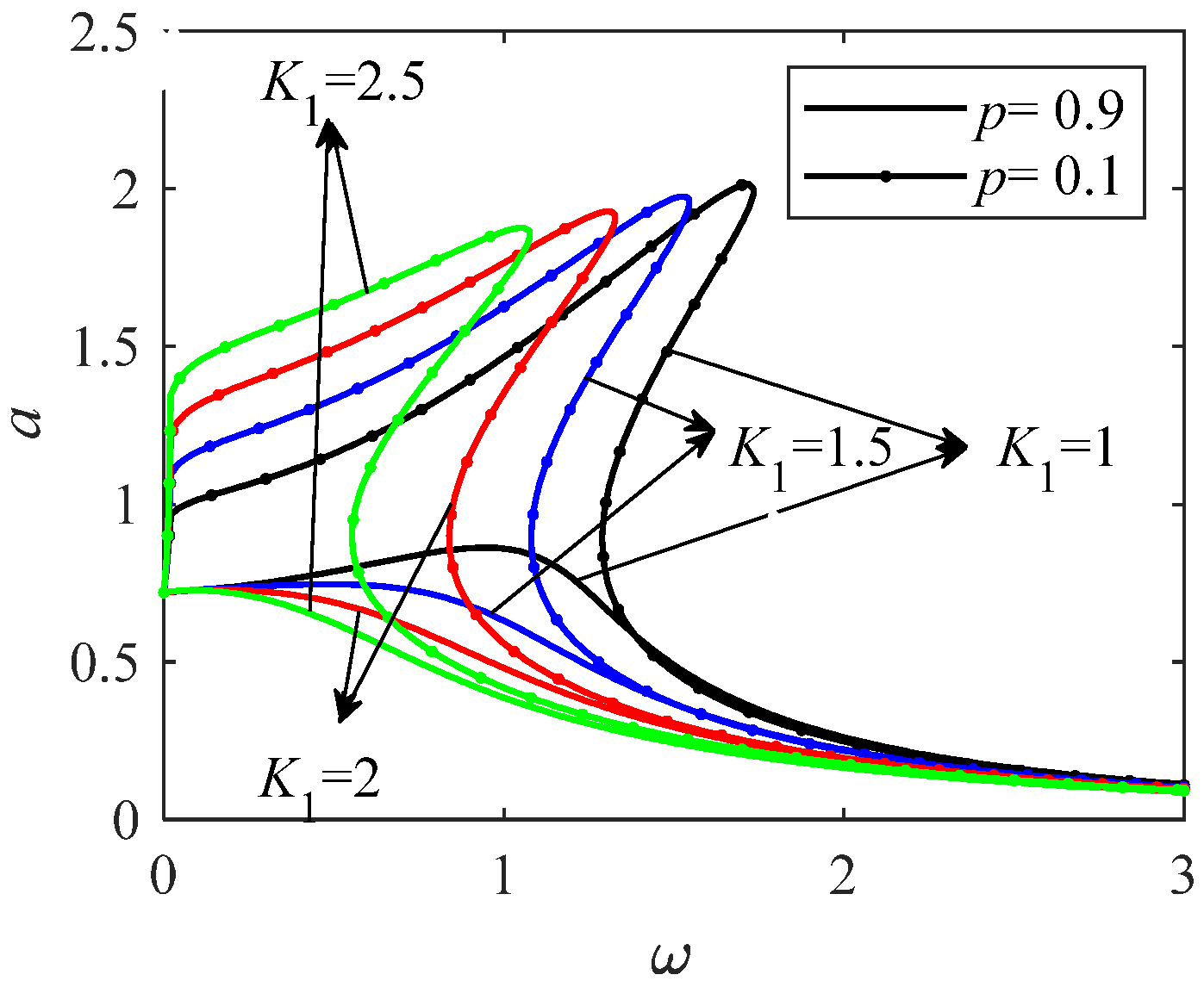
The effect of K on the amplitude–frequency curves at p = 0.9 and p = 0.1.

Figure 8.
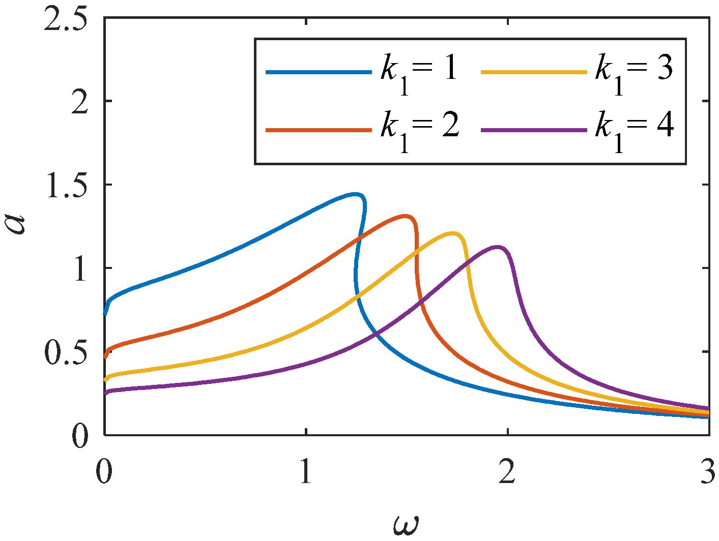
Amplitude–frequency curve when k1 changes (K = 1, p = 0.33).
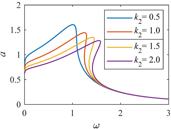
Figure 9.
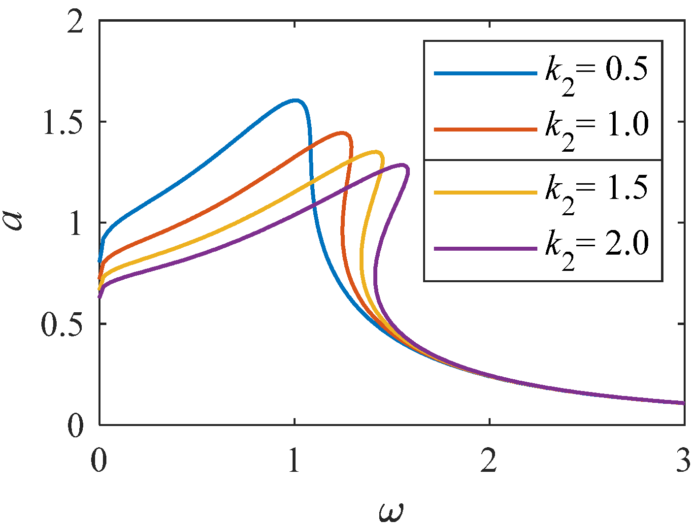
Amplitude–frequency curve when k2 changes (K = 1, p = 0.33).
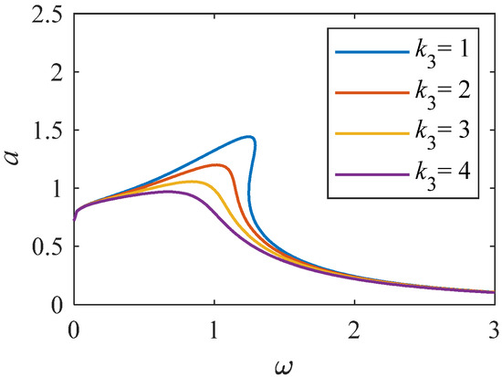
Figure 10.
Amplitude–frequency curve when k3 changes (K = 1, p = 0.33).

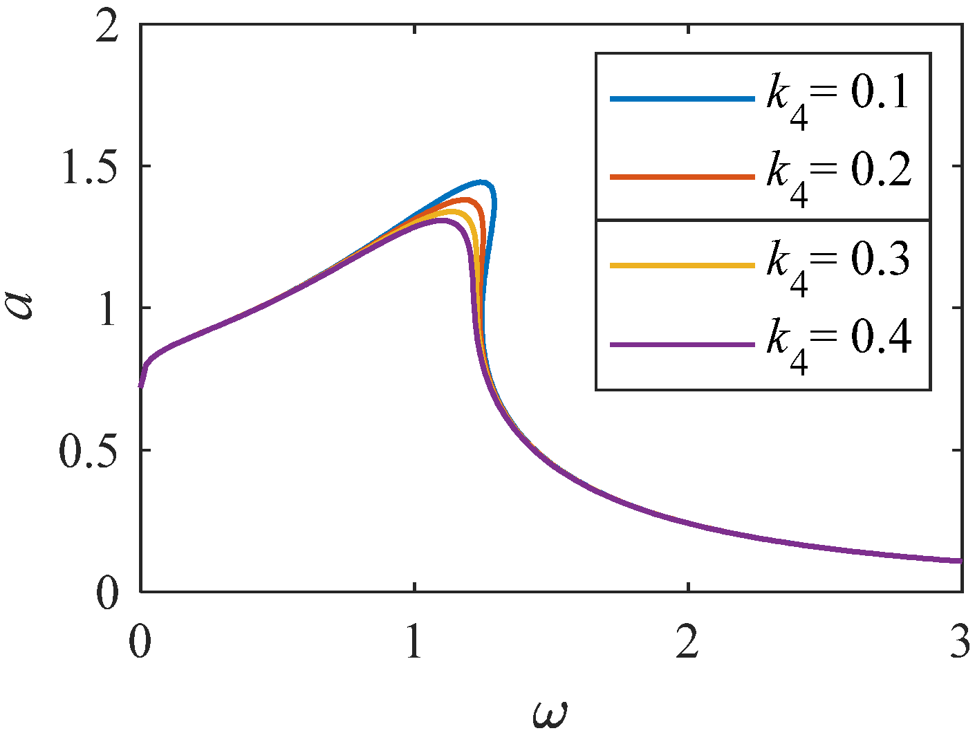
Figure 11.
Amplitude–frequency curve when k4 changes (K = 1, p = 0.33).
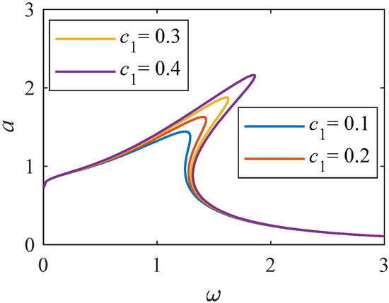
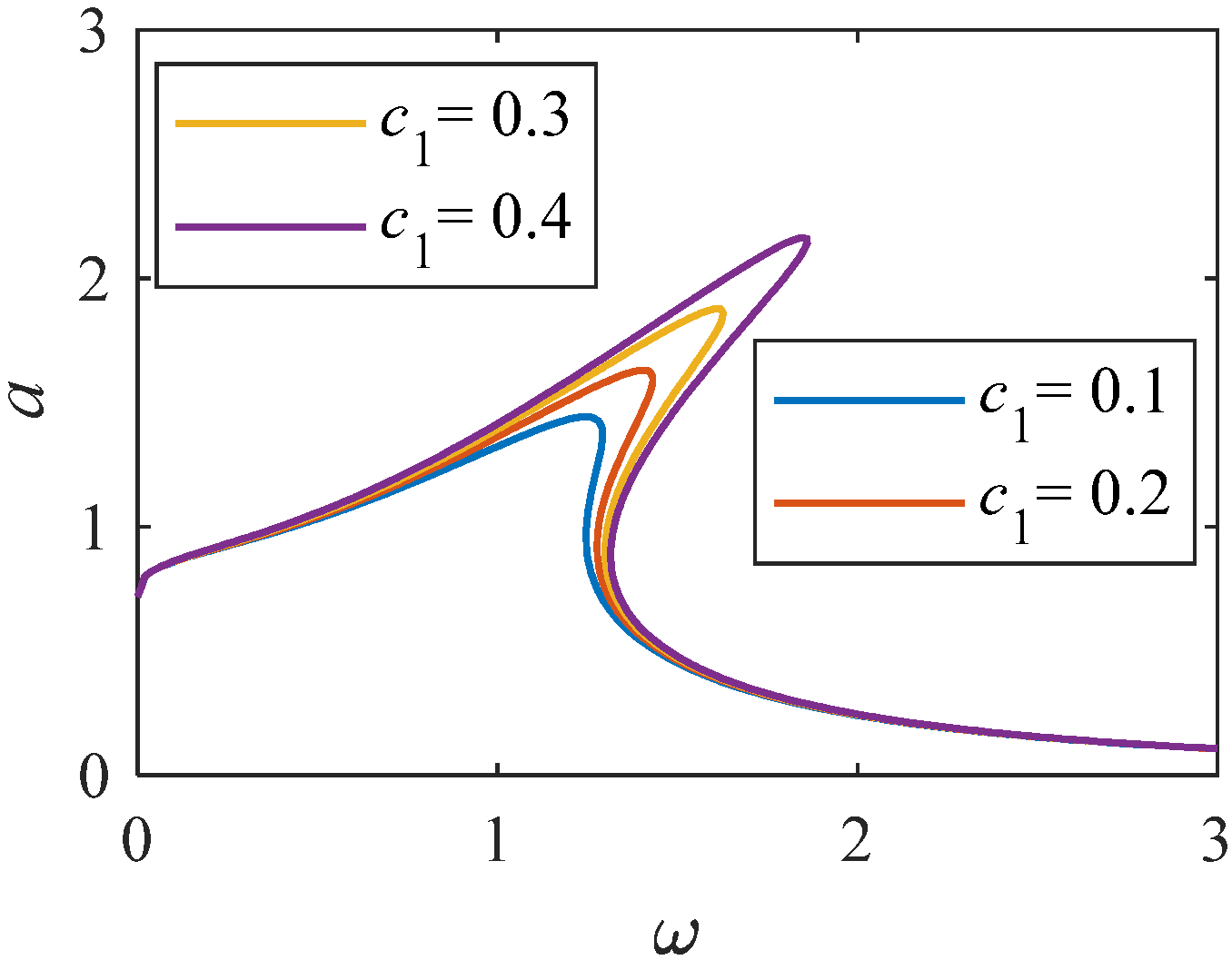
Figure 12.
Amplitude–frequency curve when c1 changes (K = 1, p = 0.33).
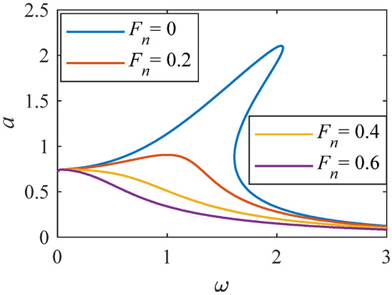
Figure 13.
Amplitude–frequency curve when Fn changes (K = 1, p = 0.33).
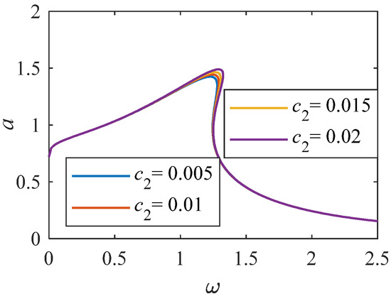
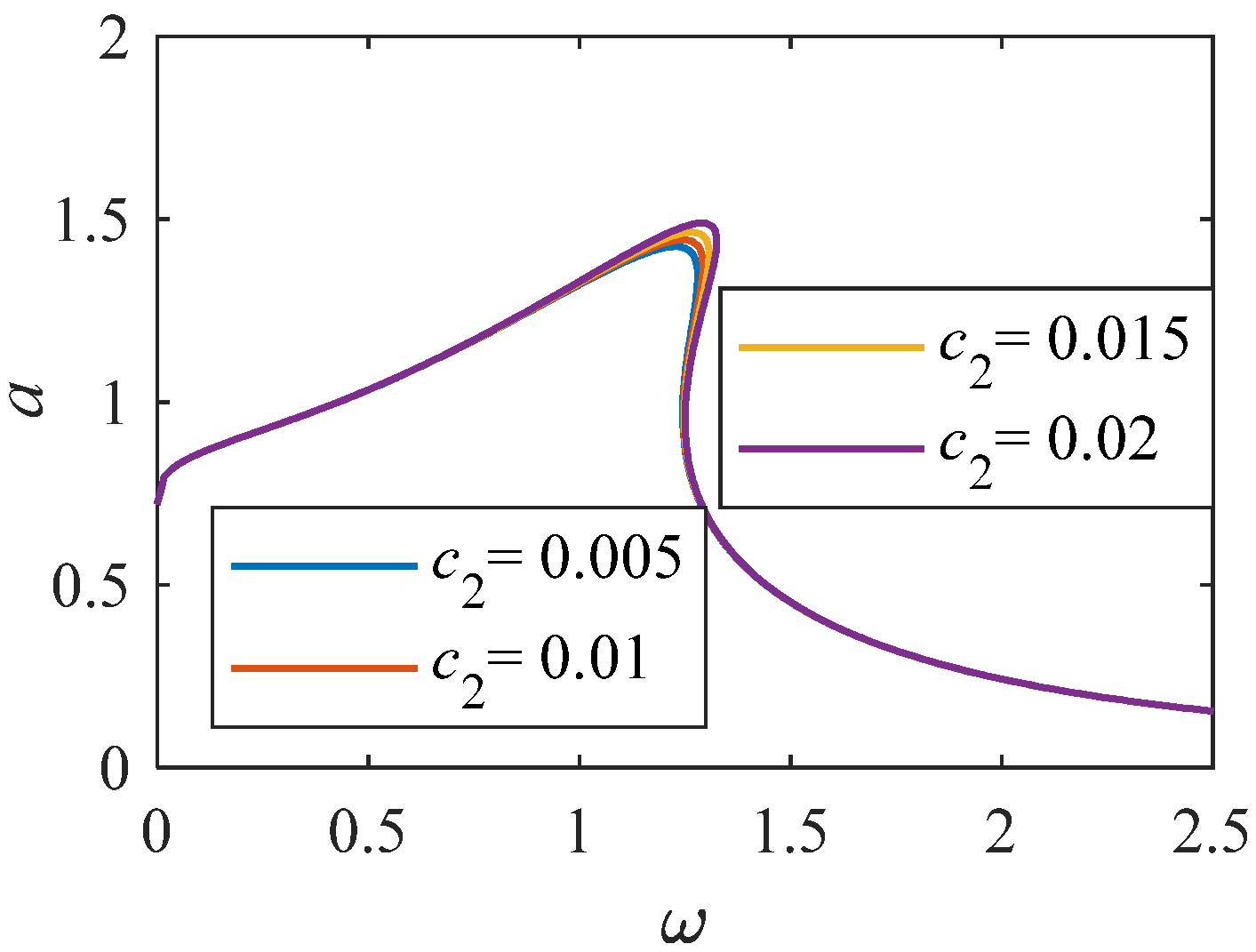
Figure 14.
Amplitude frequency curve of c2 variation range 0.005-0.02 (K = 1, p = 0.33).
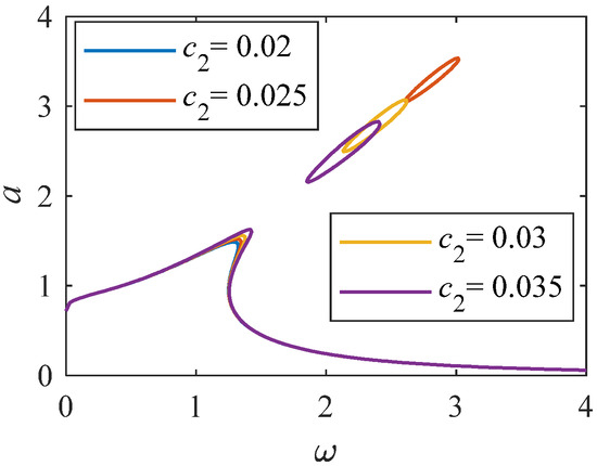
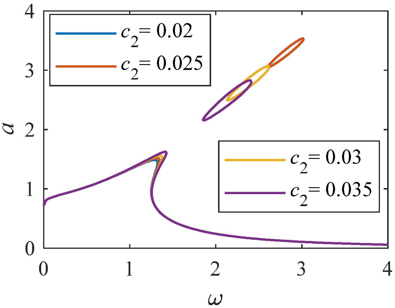
Figure 15.
Amplitude frequency curve of c2 variation range 0.02-0.035 (K = 1, p = 0.33).
From Figure 6, when K increases, the maximum value of the FOS curve decreases, the resonance interval gradually shifts to a small frequency range, and the nonlinearity weakens. It shows that the increase in K not only increases the damping of the system but also makes the system skeleton curve move to the left. When K increases, the maximum value of the relation curve between NFOS amplitude and frequency increases, and the resonance interval also changes to a small frequency range, but the nonlinearity tends to increase. When K takes the same value, the resonance interval of the FOS curve is located at the bottom left of the resonance interval of the NFOS amplitude–frequency curve. In conclusion, the vibration amplitude of FOS is smaller than that of NFOS in the resonance range.
When p is taken as a larger value, there is no unstable solution interval in the amplitude and frequency relationship curve, thus reducing the nonlinear characteristics. As the value of K increases, the peak value gradually decreases. When p is small, when K gradually changes to a larger value, the maximum amplitude gradually decreases. The resonance interval gradually moves to the low-frequency interval.
From Figure 8, we can see that when the linear stiffness gradually increases, the resonance interval gradually moves towards a higher frequency range, and the peak value gradually decreases. From Figure 9, when the value of nonlinear stiffness k2 changes to a larger value, the bending degree of the curve of the system increases, resulting in the resonance interval biased towards a higher frequency range. The results indicate that when the k2 value changes significantly, the nonlinear characteristics of the system become stronger. As shown in Figure 10 and Figure 11, when the values of k3 and k4 change significantly, the relationship curve between amplitude and frequency decreases, and the bending degree decreases gradually. It shows that the increase of k4 weakens the nonlinearity of the system, and the influence on the curve is larger than that of Figure 10 and Figure 11.
As shown in Figure 12, when the value of linear stiffness c1 changes to a larger value. The nonlinear characteristics of the system become stronger. Resonance interval tends to shift to a higher frequency range. Analyzing Figure 13, when Fn = 0, there is an unstable solution region. As Fn increases to 0.6, the system amplitude gradually decreases. When Fn is equal to 0.6, when the value of changes to a larger value, the curve of amplitude and frequency decreases. From Figure 14 and Figure 15, as increases, the system amplitude increases with the increase of c2. When c2 is greater than 0.025, an independent loop appears, and the nonlinearity is significantly enhanced.
6. Study on the Local Static Bifurcation Response Characteristics of the System
Construct the unfolding function by Equation (31):
Bifurcation point set:
Lag point set:
Hyperbolic limit point set:
After calculation:
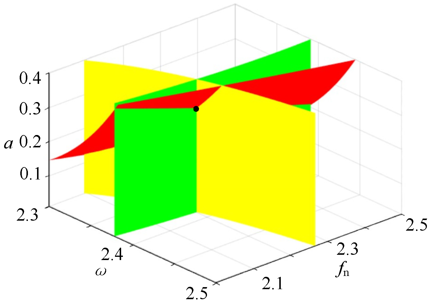
The system parameters are as follows: F0 = 1, Fn = 0.2, m = 1, k1 = 1, k2 = 1, k3 = 1, k4 = 0.1, c1 = 0.1, c2 = 0.01, K = 4, p = 0.1, vc = 0.1, and us = 0.1. The bifurcation point set and the lag point set are calculated as shown in Figure 16 and Figure 17.
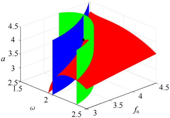
Figure 16.
Set of lag points, red represents G, green represents the first derivative of G with respect to a, and blue represents the second derivative of G with respect to a.

Figure 17.
Set of bifurcation points, red represents G, green represents the first derivative of G with respect to a, and yellow represents the first derivative of G with respect to .
As can be seen from Figure 16, the intersection point of the unfolding surface is the lag point set of the system when the current parameter value is: H = (1.706, 4.066, 3.548). According to the analysis of Figure 17, when the former parameter values are taken, the intersection point of the expanded surface is the bifurcation point set of the system: B = (2.387, 2.201, 0.3124).
By sorting Equation (37), let:
Further obtaining:
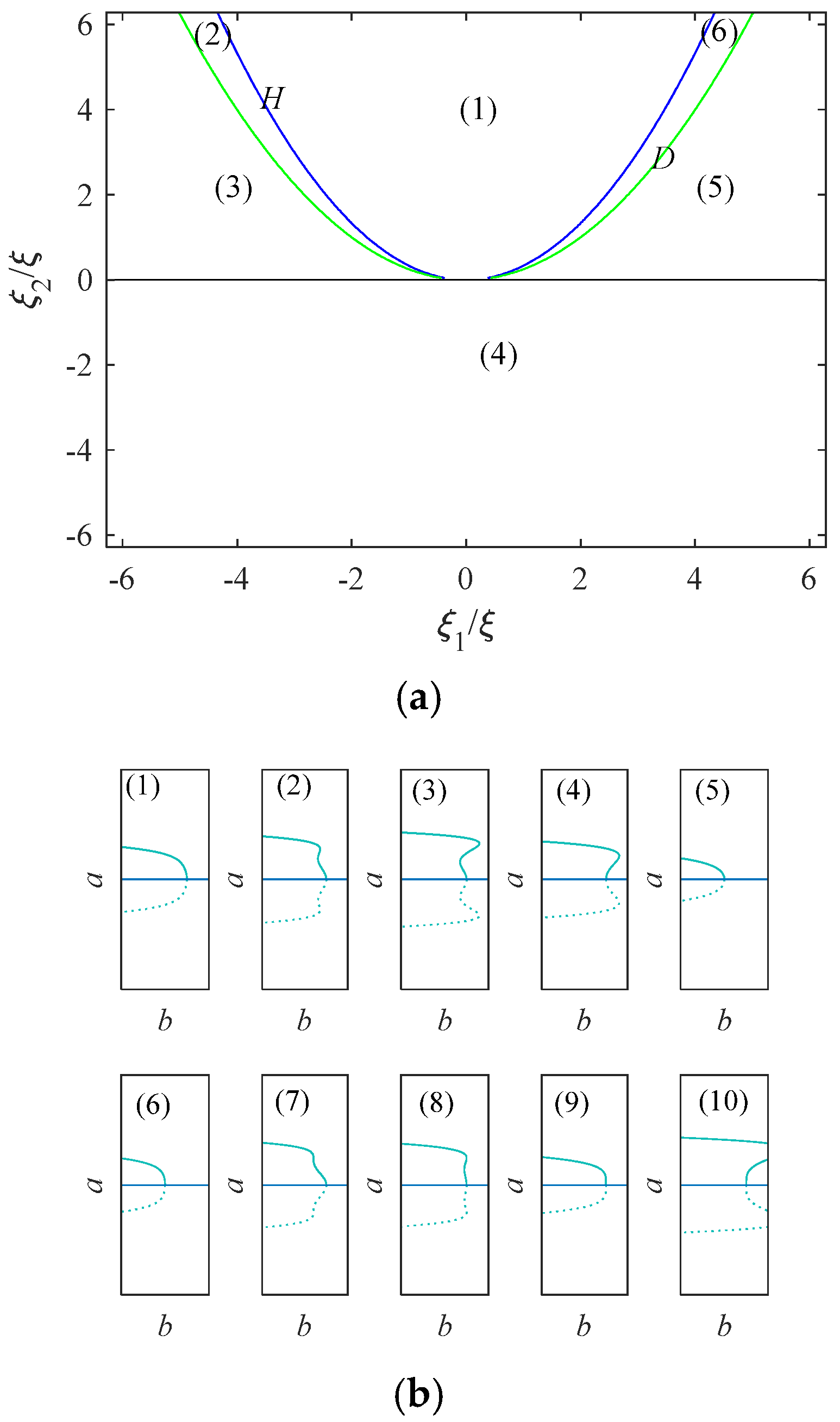
Equation (47) is a general expansion of equation ; the codimension is 2, and the system transition set is then calculated. The migration set can be represented as . Figure 8 is the system transition set and bifurcation diagram.
The parameters F0 = 1, Fn = 0.2, m = 1, k1 = 1, k2 = 1, k3 = 1, k4 = 0.1, c1 = 0.1, c2 = 0.01, K = 4, p = 0.1, vc = 0.1, and us = 0.1 are selected. The analysis of Figure 18 shows that the corresponding bifurcation topology can be obtained by taking the values of and in each region. By analyzing Figure 18b, we conclude that when the unfolding parameter passes through the transition set H from region (1) into region (2), the jump phenomenon of the system can be seen from the bifurcation topology diagram. Parts (2)–(4) in Figure 18b show different bifurcation states.
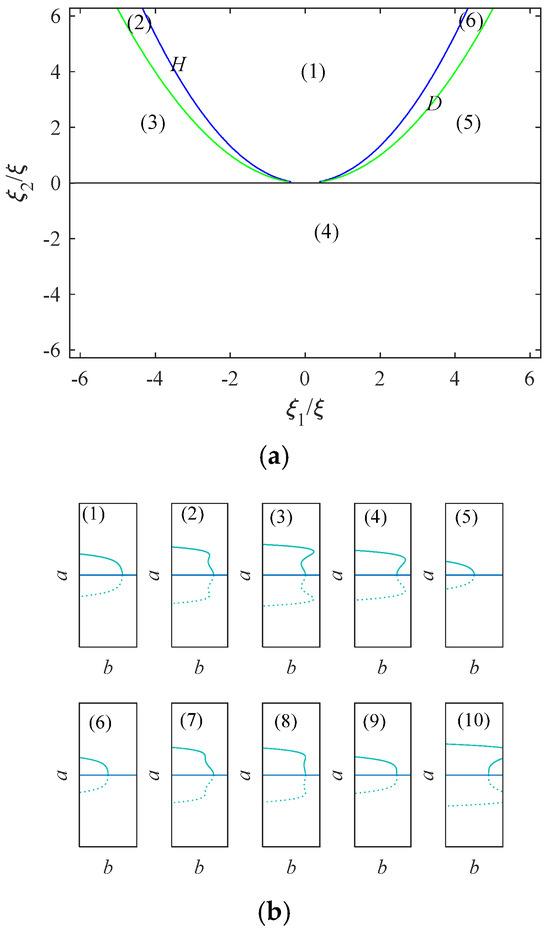
Figure 18.
(a) Transition set. (b) Bifurcation diagram.
7. Bifurcation Response Characteristics
Take a set of operating parameters of the system and conduct bifurcation research with the following parameter values: F0 = 1, m = 1, k1 = 1, k2 = 1, k3 = 1, k4 = 0.1, c1 = 0.1, p = 0.1, vc = 0.1, and us = 0.1.
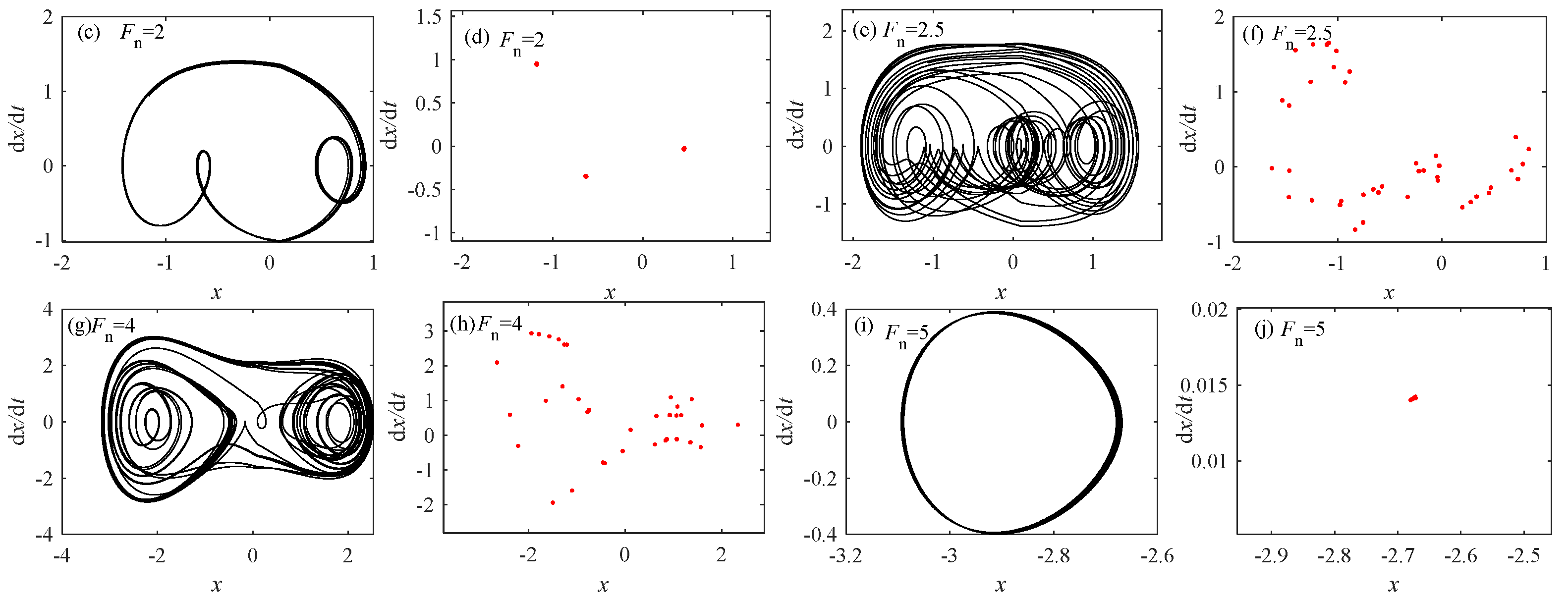
From Figure 19, it can be seen that when Fn changes, the motion is different. When the Fn value increases, the system state initially undergoes generalized three-period motion and then becomes a large-scale chaotic state. It was not until Fn became 4.2 that it transitioned to a small degree of chaotic motion. When in a chaotic state, the corresponding LLE graph value is also greater than 0. The Fn values of different motion states are taken below; the diagrams and Poincaré diagrams are drawn to verify different motion states.
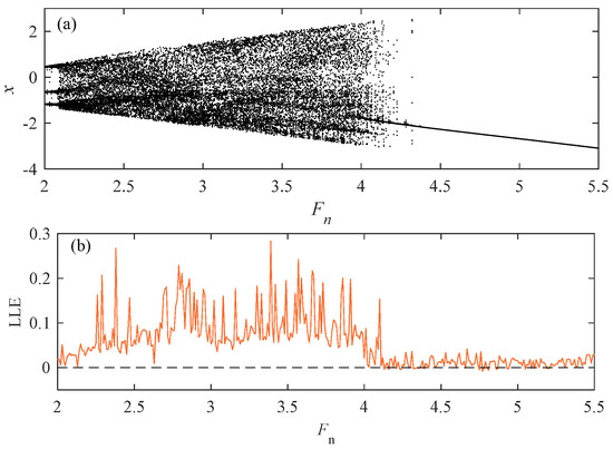
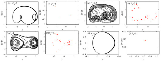
Figure 19.
When c2 = 0.01, = 1.8, and K = 0.5. (a) Bifurcation diagram; (b) Largest Lyapunov Exponent (LLE); (c) phase diagram at Fn = 2; (d) Poincaré sections at Fn = 2; (e) phase diagram at Fn = 2.5; (f) Poincaré sections at Fn = 2.5; (g) phase diagram at Fn = 4; (h) Poincaré sections at Fn = 4; (i) phase diagram at Fn = 5; and (j) Poincaré sections at Fn = 5.

Table 1.
The motion state when Fn takes different values.
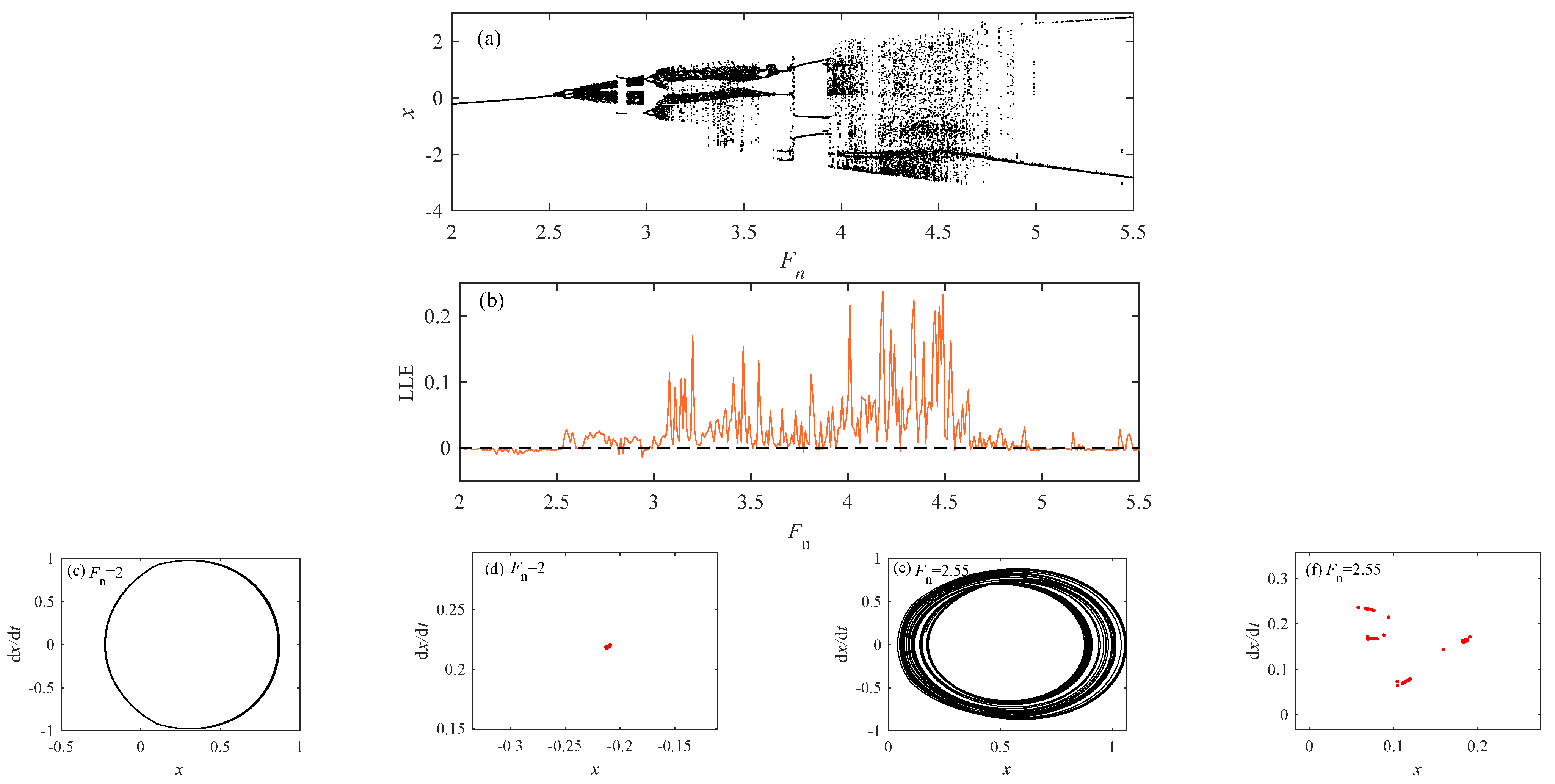
From Figure 20, it can be seen that when K changes, it shows a different motion state from Figure 19. When the value of Fn changes to a larger value, the state is a single cycle → chaotic state → two period motion → chaotic state → three period motion → chaos → single period motion. Compared with K = 0.5, the system state is more abundant at K = 1.5. In a single cycle state, the LLE value is less than 0, while the value of LLE in other motion states is greater than 0. The Fn values of different motion states are 2, 2.55, 2.6, 2.71, 2.88, 3.5, 3.8, and 4.35, respectively. The diagrams and Poincaré sections are drawn to verify different motion states.
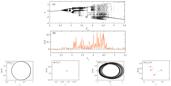
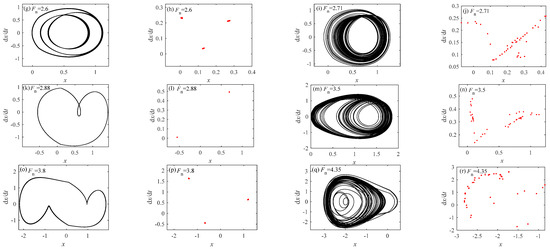
Figure 20.
When c2 = 0.01, = 1.8, and K = 1.5. (a) Bifurcation diagram; (b) LLE; (c) phase diagram at Fn = 2; (d) Poincaré sections at Fn = 2; (e) phase diagram at Fn = 2.55; (f) Poincaré sections at Fn = 2.55; (g) phase diagram at Fn = 2.6; (h) Poincaré sections at Fn = 2.6; (i) phase diagram at Fn = 2.71; (j) Poincaré sections at Fn = 2.71; (k) phase diagram at Fn = 2.88; (l) Poincaré sections at Fn = 2.88; (m) phase diagram at Fn = 3.5; (n) Poincaré sections at Fn = 3.5; (o) phase diagram at Fn = 3.8; (p) Poincaré sections at Fn = 3.8; (q) phase diagram at Fn = 4.35; (r) Poincaré sections at Fn = 4.35.
Table 2.
Each typical point and motion state when Fn takes different values.
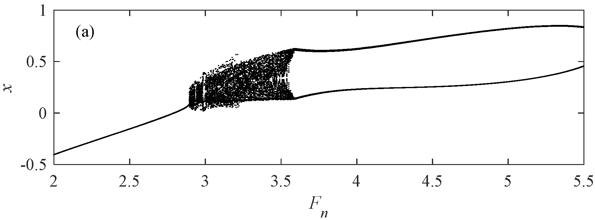
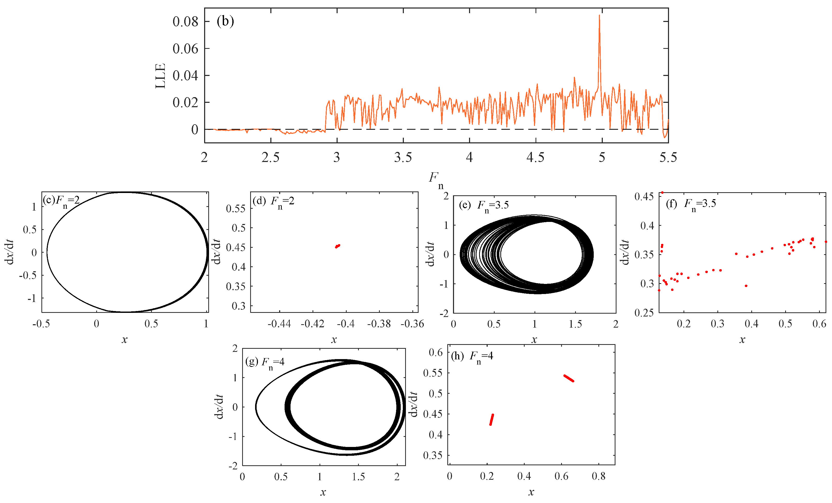
It can be seen from Figure 21 that when K is equal to 2, when Fn increases, the system changes in the order of single period → chaotic state → two-period motion. In a single cycle state, the value of LLE is less than 0, while the value of LLE in other motion states is greater than 0. Next, Fn values of different motion states are taken as 2, 3.5, and 4, respectively, and the picture and Poincaré sections are calculated to verify different motion states of the system.

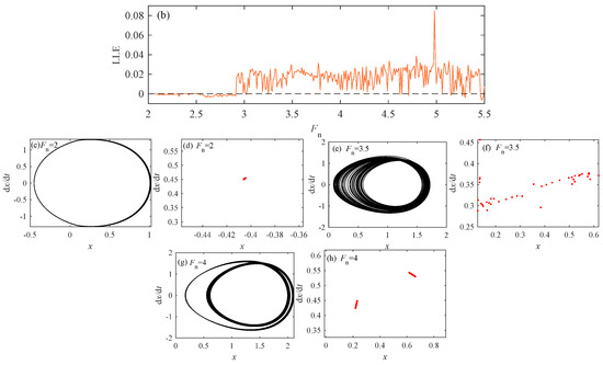
Figure 21.
When c2 = 0.01, = 1.8, and K = 2. (a) Bifurcation diagram; (b) LLE; (c) phase diagram at Fn = 2; (d) Poincaré sections at Fn = 2; (e) phase diagram at Fn = 3.5; (f) Poincaré sections at Fn = 3.5; (g) phase diagram at Fn = 4; (h) Poincaré sections at Fn = 4.
Table 3.
Each typical point and motion state when Fn takes different values.
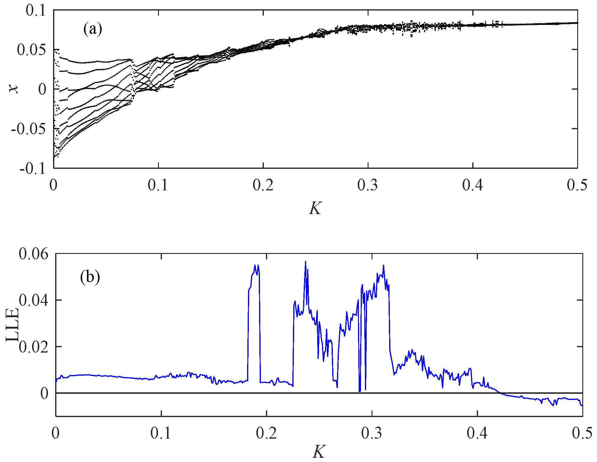
Finally, to visually demonstrate the impact of fractional order on bifurcation, we selected K as the bifurcation parameter in our study.
Analyzing Figure 22, the system exhibits a variety of rich motion phenomena, including various periodic motion states. Our ultimate goal is to maintain the motion within a single-cycle state. A bifurcation diagram within this range shows that the system moves in one period, and the maximum Liapunov curve shows that the LLE value at this time is less than 0.
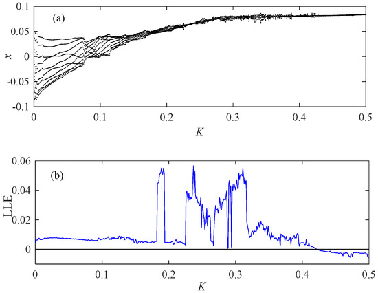
Figure 22.
When Fn = 0.5 and p = 0.33. (a) Bifurcation diagram; (b) LLE.
8. Conclusions
In this study, we conducted in-depth research on a type of friction system. By applying fractional calculus to viscoelastic systems, we have successfully described their unique dynamic characteristics. We derived the equations for system amplitude and frequency using a nonlinear approximate analytical algorithm (averaging method) and verified the effectiveness of the analytical solution through power series expansion. By comparing the amplitude frequency curves of FOS and NFOS, we found that adding fractional order terms can effectively reduce the vibration amplitude, reduce the nonlinear characteristics of the system, and narrow down the range of unstable solutions of the system.
We analyzed in detail the effects of damping parameters, stiffness parameters, fractional order parameters, and disturbance parameters on the amplitude frequency curve. Research has found that changes in system parameter values can lead to significant changes in amplitude frequency curves and stability, providing a theoretical basis for material selection in system production. In addition, we investigated the local static bifurcation response and obtained the law of bifurcation characteristics changing with the opening parameters. Furthermore, we investigated the dynamic bifurcation behavior under different parameter perturbations, and the results showed that changing the system parameters would cause the system to alternate between single-period motion, multi-period motion, and chaotic motion. Therefore, by controlling the system parameters, we can maintain the system within the periodic motion range, thereby improving the stability of the system.
In order to better describe the response of the braking system and improve its performance, we propose the following suggestions:
- Adjust fractional order parameters to optimize the vibration characteristics of the system, thereby reducing unnecessary energy loss.
- Based on the amplitude frequency curve, select damping and stiffness parameters reasonably to ensure that the system remains stable under predetermined operating conditions.
By controlling the disturbance parameters, the system can avoid entering an unstable or chaotic state and improve the reliability and performance of the braking system.
The advantages and disadvantages of using fractional derivatives for viscoelastic materials in dynamic models are summarized as follows:
- Advantages: (1) Fractional calculus can more accurately describe the memory characteristics and time dependence of viscoelastic materials. (2) Fractional calculus provides a more flexible tool to simulate the complex dynamic behavior of different materials.
- Disadvantages: (1) Compared with integer order calculus, fractional order calculus has more complex calculations, especially in numerical calculations. This may lead to a decrease in computational efficiency, especially when processing large-scale data or conducting real-time simulations. (2) The theoretical foundation of fractional calculus is still relatively weak. The approximate processing of fractional calculus may lead to errors in the results, and further verification and improvement are needed in future research.
Author Contributions
Conceptualization, data curation, visualization, writing—original draft, methodology, and formal analysis: W.M. Project administration, investigation, and supervision: Q.D. Software, writing—review and editing, and validation: W.L. Funding acquisition and resources: Z.Y. All authors have read and agreed to the published version of the manuscript.
Funding
This research was funded by the Jilin Province Science and Technology Development Plan Project (20240302038GX) and the Beijing Enterprise Horizontal Project (3R2205502419).
Data Availability Statement
The data presented in this study are available upon request from the corresponding author.
Conflicts of Interest
Author Zhenqi Yang was employed by the company State Grid Jibei Electric Power Co., Ltd. The remaining authors declare that the research was conducted in the absence of any commercial or financial relationships that could be construed as a potential conflict of interest.
References
- Mahdi, H.; Akgun, S.A.; Saleh, S.; Dautenhahn, K. A survey on the design and evolution of social robots—Past, present and future. Robot. Auton. Syst. 2022, 156, 104193. [Google Scholar] [CrossRef]
- Shah, A. Emerging trends in robotic aided additive manufacturing. In Proceedings of the International Conference on Additive Manufacturing and Advanced Materials (AM2), Gandhinagar, India, 6 January 2022. [Google Scholar] [CrossRef]
- Zbiss, K.; Kacem, A.; Santillo, M.; Mohammadi, A. Automatic Collision-Free Trajectory Generation for Collaborative Robotic Car-Painting. IEEE Access 2022, 10, 9950–9959. [Google Scholar] [CrossRef]
- Ju, H.; Park, H.; Kim, N.; Lim, J.; Jung, D.; Lee, J. A Locally Actuatable Soft Robotic Film for Actively Reconfiguring Shapes of Flexible Electronics. Soft Robot. 2022, 9, 767–775. [Google Scholar] [CrossRef] [PubMed]
- Volpe, G.; Cohen, S.; Capps, R.C.; Giacomelli, B.; McManus, R.; Scheckelhoff, K.; Choudhary, K.; Dabestani, A.T.; Hermann, S.; Kuiper, S.; et al. Robotics in acute care hospitals. Am. J. Health Syst. Pharm. 2012, 69, 1601–1603. [Google Scholar] [CrossRef]
- Oran, I.B.; Cezayirlioglu, H.R. AI—Robotic Applications in Logistics Industry and Savings Calculation. J. Organ. Behav. Res. 2021, 6, 148–165. [Google Scholar] [CrossRef]
- Ghiani, L.; Sassu, A.; Palumbo, F.; Mercenaro, L.; Gambella, F. In-Field Automatic Detection of Grape Bunches under a Totally Uncontrolled Environment. Sensors 2021, 21, 3908. [Google Scholar] [CrossRef] [PubMed]
- Liu, X.-F.; Zhang, X.-Y.; Cai, G.-P.; Chen, W.-J. Capturing a Space Target Using a Flexible Space Robot. Appl. Sci. 2022, 12, 984. [Google Scholar] [CrossRef]
- Bocii, L.S.; Sanjuan, J.J.V. Determination of the Braking Characteristics in Case of the Variation Depending on the Temperature of the Material Properties of the Friction Coupling of the Disc Brake of Railway Vehicles. Acta Tech. Napoc. Ser. Appl. Math. Mech. Eng. 2022, 65, 125–134. [Google Scholar]
- Zhang, W.; Zhao, C.; Chen, P.; Chen, E.; Lei, T. Numerical simulation and experimental research on mechanical behaviour of hydraulic disc brakes based on multi-body dynamics. Sci. Rep. 2022, 12, 18594. [Google Scholar] [CrossRef]
- Zhou, S.; Wang, Q.; Liu, J. Control Strategy and Simulation of the Regenerative Braking of an Electric Vehicle Based on an Electromechanical Brake. Trans. Famena 2022, 46, 23–40. [Google Scholar] [CrossRef]
- Yuan, Q. Study on the Influence of Damping Shim on Friction Squeal Characteristics of Automobile Disc Brakes. Noise Vib. Control 2022, 42, 201–207. [Google Scholar]
- Liu, S.H.; Wang, Z.T.; Ren, Y.R.; Ning, K.Y.; Yang, L.L. Research on full-stroke transfer coefficient of brake’s ball-plate forcing mechanism. J. Mach. Des. 2022, 39, 7–12. [Google Scholar]
- Suo, R.; Shi, X. Temperature Field and Stress Field Distribution of Forged Steel Brake Disc for High speed Train. Jordan J. Mech. Ind. Eng. 2022, 16, 113–121. [Google Scholar]
- Christian, S. Canadian space robotic activities. Acta Astronaut. 2004, 41, 239–246. [Google Scholar] [CrossRef]
- Verzijden, P. ERA performance measurements test results. In Proceedings of the 7th ESA Workshop on Advanced Space Technologies for Robotics and Automation ‘ASTRA 2002′ ESTEC, Noordwijk, The Netherlands, 19–21 November 2002. [Google Scholar]
- Shao, Z.Y.; Sun, H.X.; Jia, Q.X. Development of a general 2-dof space module. In Proceedings of the IEEE/RSJ International Conference on Intelligent Robots and Systems, Beijing, China, 9–15 October 2006; pp. 1002–1007. [Google Scholar] [CrossRef]
- Podlubny, I. Chapter 3—Existence and Uniqueness Theorems. In Mathematics in Science and Engineering; Elsevier: Amsterdam, The Netherlands, 1999; Volume 198, pp. 121–136. [Google Scholar] [CrossRef]
- Podlubny, I. Chapter 10—Survey of Applications of the Fractional Calculus. In Mathematics in Science and Engineering; Elsevier: Amsterdam, The Netherlands, 1999; Volume 198, pp. 261–307. [Google Scholar] [CrossRef]
- Podlubny, I. Chapter 9—Fractional-order Systems and Controllers. In Mathematics in Science and Engineering; Elsevier: Amsterdam, The Netherlands, 1999; Volume 198, pp. 243–260. [Google Scholar] [CrossRef]
- Song, Y.; Wang, H.; Chang, Y.; Li, Y. Nonlinear creep model and parameter identification of mudstone based on a modified fractional viscous body. Environ. Earth Sci. 2019, 78, 607. [Google Scholar] [CrossRef]
- Di Paola, M.; Alotta, G.; Burlon, A.; Failla, G. A novel approach to nonlinear variable-order fractional viscoelasticity. Philos. Trans. R. Soc. A Math. Phys. Eng. Sci. 2020, 378, 20190296. [Google Scholar] [CrossRef] [PubMed]
- Mezhoud, R.; Saoudi, K.; Zaraï, A.; Abdelmalek, S. Conditions for the local and global asymptotic stability of the time–fractional Degn–Harrison system. Int. J. Nonlinear Sci. Numer. Simul. 2020, 21, 749–759. [Google Scholar] [CrossRef]
- Birs, I.; Muresan, C.; Nascu, I.; Ionescu, C. A survey of recent advances in fractional order control for time delay systems. IEEE Access 2019, 7, 30951–30965. [Google Scholar] [CrossRef]
- Yavari, M.; Nazemi, A. On fractional infinite-horizon optimal control problems with a combination of conformable and Caputo–Fabrizio fractional derivatives. ISA Trans. 2020, 101, 78–90. [Google Scholar] [CrossRef]
- Pourhashemi, A.; Ramezani, A.; Siahi, M. Dynamic Fractional-Order Sliding Mode Strategy to Control and Stabilize Fractional-Order Nonlinear Biological Systems. IETE J. Research 2020, 68, 2560–2570. [Google Scholar] [CrossRef]
- Tran, N.; Van Au, V.; Zhou, Y.; Tuan, N.H. On a final value problem for fractional reaction-diffusion equation with Riemann-Liouville fractional derivative. Math. Methods Appl. Sci. 2020, 43, 3086–3098. [Google Scholar] [CrossRef]
- Marco, A.; Prabakaran, B.; Ivan, B. Anisotropic fractional viscoelastic constitutive models for human descending thoracic aortas. J. Mech. Behav. Biomed. Mater. 2019, 99, 186–197. [Google Scholar] [CrossRef]
- Lin, Z.L.; Zhang, J.Y.; He, L.Z. Method of Multiple Low-order Harmonic Currents Suppression Based on Fractional-order Capacitor. In Proceedings of the Chinese Society For Electrical Engineering, Wuhan, China, 9 February 2022; Volume 42, pp. 8921–8932. [Google Scholar] [CrossRef]
- Zhuang, B.; Cui, B.T.; Lou, X.Y.; Chen, J. Backstepping-based Output Feedback Boundary Control for Coupled Fractional Reaction-diffusion Systems. Acta Autom. Sin. 2022, 48, 2729–2743. [Google Scholar] [CrossRef]
- Zhu, H.H.; Zhu, J.Z.; Li, S.L.; Fan, J.W.; Done, H.J.; Wu, W.L. Power flow calculation and voltage analysis of fractional order power system. Electr. Mach. Control 2022, 26, 38–46. [Google Scholar] [CrossRef]
- Lu, C.H.; Bai, H.B. Study on Constitutive Model of Viscoelastic Material. Polym. Mater. Sci. Eng. 2007, 23, 28–31. [Google Scholar]
- Dai, J.; Han, M.; Ang, K.K. Moving element analysis of partially filled freight trains subject to abrupt braking. Int. J. Mech. Sci. 2019, 151, 85–94. [Google Scholar] [CrossRef]
- Wu, Q.; Luo, S.; Cole, C. Longitudinal dynamics and energy analysis for heavy haul trains. J. Mod. Transp. 2014, 22, 127–136. [Google Scholar] [CrossRef]
- Mastroddi, F.; Martarelli, F.; Eugeni, M.; Riso, C. Time- and frequency-domain linear viscoelastic modeling of highly damped aerospace structures. Mech. Syst. Signal Process. 2019, 122, 42–55. [Google Scholar] [CrossRef]
- He, Y.; Li, H.B.; Du, J. Dynamic Modulus Fitting Method of Viscoelastic Materials Based on Complex Neural Network. Chin. Q. Mech. 2022, 43, 406–415. [Google Scholar] [CrossRef]
- Li, M.M.; Fang, B.; Zhen, Y.X.; Zhao, J.X. A hybrid vibration isolator based on piezoelectric and viscoelastic materials. J. Vib. Shock 2017, 36, 134–140. [Google Scholar] [CrossRef]
- Tang, Z.H.; Luo, G.H.; Chen, W.; Yang, G.; Fang, J. Parallel dynamic model of rubber isolator about five-parameter fractional derivatives. J. Aerodyn. 2013, 28, 275–282. [Google Scholar] [CrossRef]
- Chang, Y.J.; Tian, W.W.; Chen, E.L.; Shen, Y.J.; Xing, W.C. Dynamic model for the nonlinear hysteresis of metal rubber based on the fractional-order derivative. Vib. Shock 2020, 39, 233–241. [Google Scholar] [CrossRef]
- Hamed, Y.S.; Albogamy, K.M.; Sayed, M. Nonlinear vibrations control of a contact-mode AFM model via a time-delayed positive position feedback. AEJ Alex. Eng. J. 2021, 60, 963–977. [Google Scholar] [CrossRef]
- Kandil, A.; Sayed, M.; Saeed, N.A. On the nonlinear dynamics of constant stiffness coefficients 16-pole rotor active magnetic bearings system. Eur. J. Mech. A/Solids 2020, 84, 104051. [Google Scholar] [CrossRef]
- Ms, A.; Aamb, C.; Imd, E. Stability and bifurcation analysis of a buckled beam via active control. Appl. Math. Model. 2020, 82, 649–665. [Google Scholar] [CrossRef]
- Wang, K. Stability and approximate solution of nonlinear dynamic system of a cylinder with two end faces in relative rotation. Acta Phys. Sin. 2005, 54, 5530–5533. [Google Scholar] [CrossRef]
- Wang, K.; Guan, X.P.; Qiao, J.M. Precise periodic solutions and uniqueness of periodic solutions of some relative rotation nonlinear dynamic system. Acta Phys. Sin. 2010, 59, 3648–3653. [Google Scholar] [CrossRef]
- Podlubny, I. Chapter 2—Fractional Derivatives and Integrals. In Mathematics in Science and Engineering; Elsevier: Amsterdam, The Netherlands, 1999; Volume 198, pp. 41–119. [Google Scholar] [CrossRef]


Disclaimer/Publisher’s Note: The statements, opinions and data contained in all publications are solely those of the individual author(s) and contributor(s) and not of MDPI and/or the editor(s). MDPI and/or the editor(s) disclaim responsibility for any injury to people or property resulting from any ideas, methods, instructions or products referred to in the content. |
© 2024 by the authors. Licensee MDPI, Basel, Switzerland. This article is an open access article distributed under the terms and conditions of the Creative Commons Attribution (CC BY) license (https://creativecommons.org/licenses/by/4.0/).