New Event-Triggered Synchronization Criteria for Fractional-Order Complex-Valued Neural Networks with Additive Time-Varying Delays

Abstract

This paper explores the synchronization control issue for a class of fractional-order Complex-valued Neural Networks (FOCVNNs) with additive time-varying delays (TVDs) utilizing a sampled-data-based event-triggered mechanism (SDBETM). First, an innovative free-matrix-based fractional-order integral inequality (FMBFOII) and an improved fractional-order complex-valued integral inequality (FOCVII) are proposed, which are less conservative than the existing classical fractional-order integral inequality (FOII). Secondly, an SDBETM is inducted to conserve network resources. In addition, a novel Lyapunov–Krasovskii functional (LKF) enriched with additional information regarding the fractional-order derivative, additive TVDs, and triggering instants is constructed. Then, through the integration of the innovative FOCVII, LKF, SDBETM, and other analytical methodologies, we deduce two criteria in the form of linear matrix inequalities (LMIs) to ensure the synchronization of the master–slave FOCVNNs. Finally, numerical simulations are illustrated to confirm the validity of the proposed results.

1. Introduction

Real-valued Neural Networks (RVNNs) have seen widespread adoption across numerous engineering disciplines, such as pattern recognition, robot control, automatic control, information processing, secure communication, and predictive estimation [1,2,3,4]. As scientific progress accelerates, complex-valued signals are frequently encountered across various domains, holding important practical significance. Thus, Complex-valued Neural Networks (CVNNs) have been introduced. Differing from RVNNs, CVNNs excel in addressing numerous challenges that RVNNs struggle with; examples include the symmetric detection problem and the XOR problem [5,6,7]. Furthermore, CVNNs demonstrate exceptional capability in handling complex-valued data due to the neuron states, inputs, weights, and activation functions all taking complex values. Thus, CVNNs have been of considerable interest and have been widely used in the spheres of quantum waves, neural cryptography, and pattern classification [8,9]. In recent years, the infinite memory and hereditary properties of fractional-order systems have attracted significant attention and spurred research across various fields [10,11,12]. Notably, some researchers have integrated fractional-order algorithms with complex-valued neural networks (CVNNs), resulting in the development of FOCVNNs. This has led to extensive investigations into the dynamic behavior of these systems [13,14,15]. Furthermore, the unavoidable time delay in neuronal information transmission can potentially induce instability, bifurcation, and oscillations within neural networks (NNs) [5,8,9]. Hence, investigating FOCVNNs incorporating time delays is crucial.

On the flip side, signals transmitted between locations traverse multiple network segments, each presenting different transmission conditions, which makes some delays that seem to be of the same type have different characteristics due to various factors [5,16]. For instance, in feedback control systems, the distinct placements of the physical plant, controller, sensor, and actuator result in two additive TVDs with differing characteristics. These delays emerge during the transmission of signals from sensor to controller and from controller to actuator [5]. It is unreasonable to discuss these two delays simply as a whole. Consequently, studying the stability of NNs with additive TVDs is paramount, as it has become the focal point of discussion. For example, ref. [8] investigated the global asymptotic stability for CVNNs with additive TVDs, employing the newly proposed double and triple complex-valued Jenson integral inequality. Ref. [5] examined CVNNs with two additive TVDs, utilizing Jenson’s integral inequality in conjunction with the reciprocally convex combination inequality and state estimation method. Ref. [16] discussed stochastic stability for neutral-type NNs with uncertain semi-Markovian jumps and additive TVDs using an extended reciprocally convex combination inequality. The robust stability for stochastic CVNNs with uncertainty and additive TVDs is investigated in [17] through the utilization of integral inequalities and the construction of an LKF that incorporates information regarding additive TVDs. Although many research results on CVNNs with additive TVDs have been published in recent years, research findings on FOCVNNs with additive TVDs are scarce. Consequently, it is valuable to investigate FOCVNNs with additive TVDs.

In addition, LMI methods and LKFs are widely used in the study of system stability [18,19]. However, when applying these methods, a key challenge arises: how to reduce conservatism. Generally, there are two approaches to address this issue: one is to construct more complex LKFs; the other is to relax the derivatives of the LKFs using integral inequality techniques. As we all know, the integral inequality method plays a crucial role in reducing the conservatism of stability conditions or synchronization criteria for various kinds of delayed systems, and it has attracted much more attention in recent years [11,20,21]. However, by the force of the intricacies in fractional-order systems (FOSs), conventional integer-order integral inequalities are rendered inapplicable, so it is imperative to formulate the corresponding FOII for analyzing FOSs. In pursuit of this goal, numerous scholars have dedicated considerable efforts to advancing and refining integral inequalities, such as the fractional-order Jenson integral inequality [1,4], Wirtinger-based fractional-order integral inequality (WBFOII) [4,22], and FMBFOII [4,23,24]. Scholars have derived numerous valuable findings from the aforementioned FOIIs. For example, in reference [4], a new FMBFOII was developed by using a simple auxiliary function, and it has been successfully applied to study the $H\infty$/passive state feedback control issue for delayed fractional-order gene regulatory networks. By introducing the FMBFOII and a fractional Leibniz–Newton formula, reference [23] addressed the global synchronization issue for time-invariant fractional-order NNs with time delay. Additionally, by combining a novel auxiliary function with a fractional Newton–Leibniz formula, another FMBFOII was developed in reference [24] and was employed with an SDBETM to investigate synchronization control in fractional and impulsive complex networks with switched topologies and TVDs. Despite these advancements, there are still some limitations, such as the system’s state information not being considered fully, which limits applicability to TVD systems and is not conducive to a reduction in conservatism. Moreover, the existing inequalities are real-valued, which may not be suitable for complex-valued systems. To address these issues, two new FMBFOIIs and FOCVIIs were developed by virtue of two distinct auxiliary functions and some additional free matrices, in which the information of fractional-order derivatives, TVDs, and event-triggered moments were considered fully, such that we could estimate a stricter lower bound for the derivatives of the LKF and effectively reduce conservatism in stability conditions. Additionally, although some valuable FOIIs have been proposed, there are still many deficiencies and challenges compared with traditional integer-order integral inequalities, which is a valuable research topic. Meanwhile, due to the inclusion of phase information in the state of a complex-valued system, which is unavailable in a real-valued system, studying it with real-valued inequalities presents challenges. Therefore, extending real-valued FOIIs to the complex domain is essential, offering significant value for the advancement and exploration of FOCVIIs in research and application.

Over recent years, the synchronization of NNs has emerged as the most talked-about topic, demonstrating successful applications across various fields including image encryption, signal processing, cryptography, and secure communications [25,26,27,28]. As research has progressed, various forms of synchronization of NNs have been explored, including generalized synchronization [29], complete synchronization [30], anti-synchronization [31], and projective synchronization [30]. Additionally, to achieve the control purpose, scholars have proposed control methods such as sampled-data control [1,27], event-triggered control [13,32], impulsive control [28,33,34], quantization control [35,36], and model prediction control [19], which have made significant research progress. Among them, sampled-data control has drawn a lot of attention by virtue of its ability to significantly diminish the amount of data transfer and improve the efficiency of bandwidth consumption. However, this will waste a lot of unnecessary network bandwidth resources [37]. In response to this limitation, a continuous event-triggered control method was introduced, whereby control signals are updated solely upon fulfillment of predefined event-triggered conditions [38,39]. However, the traditional event-triggering mechanism requires continuous monitoring of the system state, which can lead to excessive communication operations, unnecessary bandwidth consumption, and high computational resource usage. Therefore, an SDBETM that combines an event-triggering mechanism with a sampling mechanism, which activates events only at specific sampling instances, is proposed to address the aforementioned issues. This approach not only significantly reduces the need for continuous system monitoring but also effectively prevents the Zeno phenomenon. As a result, it conserves computational resources and increases communication efficiency. Consequently, SDBETMs have been increasingly applied in FOSs [24], NNs [40], and multi-agent systems [41]. It is worth noting that there are rarely studies on the synchronization problem of FOCVNNs with additive TVDs using SDBETMs, so this is a very worthwhile consideration.

Drawing inspiration from the preceding discussion, this paper centers on tackling the synchronization control issue within FOCVNNs with additive TVDs through the utilization of an SDBETM and FMBFOII. Below is a concise encapsulation of the primary contribution of this paper:

(1) To alleviate the conservatism in the theoretical results, a new FMBFOII is introduced and an updated FOCVII is formulated by integrating the TVD FOII described in [1];

(2) A fresh LKF is formulated based on the improved FOCVII, which fully takes advantage of the information of FD, additive TVDs, and triggering instants;

(3) By integrating the new FOCVII, LKF, and SDBETM approaches, sufficient conditions in LMIs form are established to ensure asymptotic stability for fractional-order error systems (FOEs).

Notations:

The subsequent notations are essential within this issue. $\mathbb{N}$ is an integer set. ${\mathbb{R}}^n$ stands for n-dimensional Euclidean space. ${\mathbb{C}}^n$ represents the set of n-dimensional complex-valued vectors, while ${\mathbb{C}}^{n\times m}$ represents $n\times m$ complex-valued matrices. ${\mathbb{H}}_{+}^{n\times n}$ is an $n\times n$ positive definite Hermitian matrix. H denotes the complex conjugate transpose, i is the imaginary unit, and $i=\sqrt{-1}$. The diagonal matrix is expressed as $diag\{·\}$. $Sym\left\{A\right\}$ denotes $A+A^H$, and $col\{·\}$ is a column vector. I and O denote the unit matrix and zero matrix with suitable dimensions, respectively.

2. Preliminaries

In this section, the foundational definitions and lemmas necessary for elucidating the principal findings for this issue are furnished.

Definition 1

([42]). The α-order integration of $\mathfrak{x}\left(t\right)\in {\mathbb{C}}^n$ is

$$\begin{array}{c}\hfill {\phantom{.}}_{t_0}{\mathcal{I}}_t^{\alpha }\mathfrak{x}\left(t\right)={\displaystyle \frac{1}{\Gamma \left(\alpha \right)}}{\int }_{t_0}^t{(t-s)}^{\alpha -1}\mathfrak{x}\left(s\right)ds,t>t_0,\end{array}$$

where $\alpha \in (0,1)$ and $\Gamma \left(\alpha \right)={\int }_0^{\infty }{\mathfrak{e}}^{-t}{t}^{\alpha -1}dt$ is the gamma function.

Definition 2

([42]). The Caputo α-order derivative of $\mathfrak{x}\left(t\right)\in {\mathbb{C}}^n$ is

$${\phantom{.}}_{t_0}^C{\mathcal{D}}_t^{\alpha }\mathfrak{x}\left(t\right)={\displaystyle \frac{1}{\Gamma (n-\alpha )}}{\int }_{t_0}^t{(t-s)}^{n-\alpha -1}{\mathfrak{x}}^n\left(s\right)ds,t>t_0,$$

where $\alpha \in (n-1,n]$, $n\in \mathbb{N}$. When $n=1$,

$${\phantom{.}}_{t_0}^C{\mathcal{D}}_t^{\alpha }\mathfrak{x}\left(t\right)={\displaystyle \frac{1}{\Gamma (1-\alpha )}}{\int }_{t_0}^t{(t-s)}^{-\alpha }{\mathfrak{x}}^{\prime }\left(s\right)ds.$$

For convenience, ${\phantom{.}}_{t_0}^C{\mathcal{D}}_t^{\alpha }\mathfrak{x}\left(t\right)$ is denoted as ${\phantom{.}}_{t_0}{\mathcal{D}}_t^{\alpha }\mathfrak{x}\left(t\right)$ throughout this paper.

Lemma 1

([1]). The following inequality holds for $P\in {\mathbb{H}}_{+}^{n\times n}$ and function $\mathfrak{x}\left(t\right)\in {\mathbb{C}}^n$, $t\in [a,b]$:

$$\begin{array}{cc}\hfill {\phantom{.}}_a{\mathcal{D}}_b^{\alpha }\left({\mathfrak{x}}^H\left(b\right)P\mathfrak{x}\left(b\right)\right)& ⩽2{\mathfrak{x}}^H\left(b\right)P\left({\phantom{.}}_a{\mathcal{D}}_b^{\alpha }\mathfrak{x}\left(b\right)\right).\hfill \end{array}$$

Lemma 2

([23]). The following inequality holds for function $\mathfrak{x}\left(t\right)\in {\mathbb{C}}^n$, $\forall \vartheta \in \mathbb{N}$, $[b-\vartheta ,b]\subseteq [a,b]$, and $Q\in {\mathbb{H}}_{+}^{n\times n}$:

$${\phantom{.}}_a{\mathcal{I}}_b^{\alpha }\left({\left({\phantom{.}}_a{\mathcal{D}}_b^{\alpha }\mathfrak{x}\left(b\right)\right)}^{H}Q\left({\phantom{.}}_a{\mathcal{D}}_b^{\alpha }\mathfrak{x}\left(b\right)\right)\right)⩾{\phantom{.}}_{b-\vartheta }{\mathcal{I}}_b^{\alpha }\left({\left({\phantom{.}}_a{\mathcal{D}}_b^{\alpha }\mathfrak{x}\left(b\right)\right)}^{H}Q\left({\phantom{.}}_a{\mathcal{D}}_b^{\alpha }\mathfrak{x}\left(b\right)\right)\right).$$

Lemma 3

([1]). The following inequality holds for $Q\in {\mathbb{H}}_{+}^{n\times n}$ and $\mathfrak{x}\left(t\right)\in {\mathbb{C}}^n$:

$$\begin{array}{c}\hfill {\phantom{.}}_a{\mathcal{I}}_b^{\alpha }\left({\mathfrak{x}}^H\left(b\right)Q\mathfrak{x}\left(b\right)\right)⩾{\displaystyle \frac{\Gamma (\alpha +1)}{{(b-a)}^{\alpha }}}{\left({\phantom{.}}_a{\mathcal{I}}_b^{\alpha }\mathfrak{x}\left(b\right)\right)}^{H}Q\left({\phantom{.}}_a{\mathcal{I}}_b^{\alpha }\mathfrak{x}\left(b\right)\right).\end{array}$$

(1)

Lemma 4

(WBFOII [4,22]). Suppose that $Q\in {\mathbb{H}}_{+}^{n\times n}$, for any integrable scalar function $\mathfrak{y}\left(t\right)\in {\mathbb{C}}^n,$ such that

$$\begin{array}{cc}\hfill {\phantom{.}}_a{\mathcal{I}}_b^{\alpha }\left({\left({\phantom{.}}_a{\mathcal{D}}_b^{\alpha }\mathfrak{y}\left(b\right)\right)}^{H}Q\left({\phantom{.}}_a{\mathcal{D}}_b^{\alpha }\mathfrak{y}\left(b\right)\right)\right)& ⩾{\displaystyle \frac{\Gamma (\alpha +1)}{{(b-a)}^{\alpha }}}{\Theta }_1^{H}Q{\Theta }_1+{\displaystyle \frac{3}{\Gamma (\alpha +1){(b-a)}^{\alpha }}}{\Theta }_2^{H}Q{\Theta }_2\hfill \\ \hfill & +{\displaystyle \frac{5}{\Gamma (\alpha +1){(b-a)}^{\alpha }}}{\Theta }_3^{H}Q{\Theta }_3,\hfill \end{array}$$

(2)

where

$$\begin{array}{cc}\hfill {\Theta }_1=& \mathfrak{y}\left(b\right)-\mathfrak{y}\left(a\right),{\Theta }_2={\displaystyle \frac{\Gamma (2\alpha +1)}{{(b-a)}^{\alpha }}}\phantom{.}{\phantom{.}}_a{\mathcal{I}}_b^{\alpha }\mathfrak{y}\left(b\right)-\Gamma (\alpha +1){\Theta }_1-{\displaystyle \frac{\Gamma (2\alpha +1)}{\Gamma (\alpha +1)}}\mathfrak{y}\left(a\right),\hfill \\ \hfill {\Theta }_3=& {\displaystyle \frac{2\Gamma (3\alpha +1)}{{(b-a)}^{2\alpha }}}{\phantom{.}}_a{\mathcal{I}}_b^{2\alpha }\mathfrak{y}\left(b\right)-{\displaystyle \frac{3\Gamma (2\alpha +1)}{{(b-a)}^{\alpha }}}\phantom{.}{\phantom{.}}_a{\mathcal{I}}_b^{\alpha }\mathfrak{y}\left(b\right)-\left({\displaystyle \frac{3\Gamma (2\alpha +1)}{\Gamma (\alpha +1)}}-{\displaystyle \frac{2\Gamma (3\alpha +1)}{\Gamma (2\alpha +1)}}\right)\mathfrak{y}\left(a\right)\hfill \\ \hfill +& \Gamma (\alpha +1){\Theta }_1.\hfill \end{array}$$

Lemma 5.

For function $\mathfrak{x}\left(t\right)\in {\mathbb{C}}^n,t\in [a,b]$, and any matrices $Q\in {\mathbb{H}}_{+}^{n\times n}$, $Z_1,Z_2,Z_3\in {\mathbb{H}}_{+}^{4n\times 4n}$, $Z_4,Z_5,Z_6\in {\mathbb{C}}^{4n\times 4n}$, $N_1,N_2,N_3\in {\mathbb{C}}^{4n\times n},$ such that

$$\Phi =\left[\begin{array}{cccc}{Z}_1& Z_4& Z_5& N_1\\ ★& Z_2& Z_6& N_2\\ ★& ★& Z_3& N_3\\ ★& ★& ★& Q\end{array}\right]\ge 0,$$

then

$$\begin{array}{c}\hfill -{\displaystyle \frac{1}{\Gamma \left(\alpha \right)}}{\int }_a^b{(b-s)}^{\alpha -1}{\left({\phantom{.}}_a{\mathcal{D}}_s^{\alpha }\mathfrak{x}\left(s\right)\right)}^{H}Q\left({\phantom{.}}_a{\mathcal{D}}_s^{\alpha }\mathfrak{x}\left(s\right)\right)ds⩽{\Im }^H\Omega \Im ,\end{array}$$

(3)

where

$$\begin{array}{cc}\hfill & \Im =col\left\{\mathfrak{x}\left(b\right),\mathfrak{x}\left(a\right),{\displaystyle \frac{1}{{(b-a)}^{\alpha }}}{\phantom{.}}_a{\mathcal{I}}_b^{\alpha }\mathfrak{x}\left(b\right),{\displaystyle \frac{1}{{(b-a)}^{2\alpha }}}{\phantom{.}}_a{\mathcal{I}}_b^{2\alpha }\mathfrak{x}\left(b\right)\right\},\hfill \\ \hfill & \Omega ={\displaystyle \frac{{(b-a)}^{\alpha }}{\Gamma (2-\alpha )}}\left(Z_1+{\displaystyle \frac{1}{3}}{Z}_2+{\displaystyle \frac{1}{180}}{Z}_3\right)+Sym\{N_1{\Pi }_1+N_2{\Pi }_2+N_3{\Pi }_3\},\hfill \\ \hfill & {\Pi }_1=E_1-E_2,{\Pi }_2={\displaystyle \frac{1}{\Gamma \left(\alpha \right)}}\left(2\Gamma \left(2\alpha \right)E_3-{\displaystyle \frac{2\Gamma \left(2\alpha \right)}{\Gamma (\alpha +1)}}{E}_2-\Gamma \left(\alpha \right){\Pi }_1\right),\hfill \\ \hfill & {\Pi }_3={\displaystyle \frac{1}{\Gamma \left(\alpha \right)}}\left(\Gamma \left(3\alpha \right)E_4-\Gamma \left(2\alpha \right)E_3-\left({\displaystyle \frac{\Gamma \left(3\alpha \right)}{\Gamma (2\alpha +1)}}-{\displaystyle \frac{\Gamma \left(2\alpha \right)}{\Gamma (\alpha +1)}}\right)E_2-{\displaystyle \frac{1}{6}}\Gamma \left(\alpha \right){\Pi }_1\right),\hfill \\ \hfill & E_1=\left[IOOO\right],E_2=\left[OIOO\right],E_3=\left[OOIO\right],E_4=\left[OOOI\right].\hfill \end{array}$$

Proof. 

Let $\varpi \left(s\right)=col\left\{\Im ,f\left(s\right)\Im ,g\left(s\right)\Im ,{\phantom{.}}_a{\mathcal{D}}_s^{\alpha }\mathfrak{x}\left(s\right)\right\}$ and auxiliary functions be established as below:

$$f\left(s\right)={\displaystyle \frac{2{(b-s)}^{\alpha }}{{(b-a)}^{\alpha }}}-1,g\left(s\right)={\displaystyle \frac{{(b-s)}^{2\alpha }}{{(b-a)}^{2\alpha }}}-{\displaystyle \frac{{(b-s)}^{\alpha }}{{(b-a)}^{\alpha }}}+{\displaystyle \frac{1}{6}},$$

which satisfies ${\phantom{.}}_a{\mathcal{I}}_b^{\alpha }f\left(b\right)=0,{\phantom{.}}_a{\mathcal{I}}_b^{\alpha }g\left(b\right)=0,{\phantom{.}}_a{\mathcal{I}}_b^{\alpha }f\left(b\right)g\left(b\right)=0.$

Given $\Phi \ge 0,$ then ${\varpi }^H\left(s\right)\Phi \varpi \left(s\right)\ge 0$, $\forall s\in [a,b].$ Subsequently,

$$\begin{array}{cc}\hfill {\varpi }^H\left(s\right)\Phi \varpi \left(s\right)& ={\left[\begin{array}{c}\Im \\ f\left(s\right)\Im \\ g\left(s\right)\Im \\ {\phantom{.}}_a{\mathcal{D}}_s^{\alpha }\mathfrak{x}\left(s\right)\end{array}\right]}^H\left[\begin{array}{cccc}{Z}_1& Z_4& Z_5& N_1\\ ★& Z_2& Z_6& N_2\\ ★& ★& Z_3& N_3\\ ★& ★& ★& Q\end{array}\right]\left[\begin{array}{c}\Im \\ f\left(s\right)\Im \\ g\left(s\right)\Im \\ {\phantom{.}}_a{\mathcal{D}}_s^{\alpha }\mathfrak{x}\left(s\right)\end{array}\right]\hfill \\ \hfill & ={\Im }^H{Z}_1\Im +2f\left(s\right){\Im }^H{Z}_4\Im +2g\left(s\right){\Im }^H{Z}_5\Im +{(f\left(s\right)\Im )}^H{Z}_2(f\left(s\right)\Im )\hfill \\ \hfill & +2f\left(s\right)g\left(s\right){\Im }^H{Z}_6\Im +2f\left(s\right){\Im }^H{N}_2\left({\phantom{.}}_a{\mathcal{D}}_s^{\alpha }\mathfrak{x}\left(s\right)\right)+2{\Im }^H{N}_2\left(f\left(s\right){\phantom{.}}_a{\mathcal{D}}_s^{\alpha }\mathfrak{x}\left(s\right)\right)\hfill \\ \hfill & +{(g\left(s\right)\Im )}^H{Z}_2(g\left(s\right)\Im )+2g\left(s\right){\Im }^H{N}_3\left({\phantom{.}}_a{\mathcal{D}}_s^{\alpha }\mathfrak{x}\left(s\right)\right)+{\left({\phantom{.}}_a{\mathcal{D}}_s^{\alpha }\mathfrak{x}\left(s\right)\right)}^{H}Q\left({\phantom{.}}_a{\mathcal{D}}_s^{\alpha }\mathfrak{x}\left(s\right)\right).\hfill \end{array}$$

(4)

Pre- and post-integrating (4),

$$\begin{array}{cc}\hfill {\phantom{.}}_a{\mathcal{I}}_b^{\alpha }\left({\varpi }^H\left(b\right)\Phi \varpi \left(b\right)\right)& ={\phantom{.}}_a{\mathcal{I}}_b^{\alpha }\left({\Im }^H{Z}_1\Im \right)+2{\phantom{.}}_a{\mathcal{I}}_b^{\alpha }\left(f\left(b\right){\Im }^H{Z}_4\Im \right)+2{\phantom{.}}_a{\mathcal{I}}_b^{\alpha }\left(g\left(b\right){\Im }^H{Z}_5\Im \right)\hfill \\ \hfill & +{\phantom{.}}_a{\mathcal{I}}_b^{\alpha }\left(f^2\left(b\right){\Im }^H{Z}_2\Im \right)+2{\phantom{.}}_a{\mathcal{I}}_b^{\alpha }\left({\Im }^H{N}_1\left({\phantom{.}}_a{\mathcal{D}}_b^{\alpha }\mathfrak{x}\left(b\right)\right)\right)\hfill \\ \hfill & +2{\phantom{.}}_a{\mathcal{I}}_b^{\alpha }\left(f\left(b\right)g\left(b\right){\Im }^H{Z}_6\Im \right)+2{\phantom{.}}_a{\mathcal{I}}_b^{\alpha }\left({\Im }^H{N}_2\left({\phantom{.}}_a{\mathcal{D}}_b^{\alpha }\mathfrak{x}\left(b\right)\right)\right)\hfill \\ \hfill & +{\phantom{.}}_a{\mathcal{I}}_b^{\alpha }\left(g^2\left(b\right){\Im }^H{Z}_3\Im \right)+2{\phantom{.}}_a{\mathcal{I}}_b^{\alpha }\left(f\left(b\right){\Im }^H{N}_2\left({\phantom{.}}_a{\mathcal{D}}_b^{\alpha }\mathfrak{x}\left(b\right)\right)\right)\hfill \\ & +2{\phantom{.}}_a{\mathcal{I}}_b^{\alpha }\left(g\left(b\right){\Im }^H{N}_3\left({\phantom{.}}_a{\mathcal{D}}_b^{\alpha }\mathfrak{x}\left(b\right)\right)\right)+{\phantom{.}}_a{\mathcal{I}}_b^{\alpha }\left({\left({\phantom{.}}_a{\mathcal{D}}_b^{\alpha }\mathfrak{x}\left(b\right)\right)}^{H}Q\left({\phantom{.}}_a{\mathcal{D}}_b^{\alpha }\mathfrak{x}\left(b\right)\right)\right).\hfill \end{array}$$

(5)

where

$$\begin{array}{c}\hfill {\phantom{.}}_a{\mathcal{I}}_b^{\alpha }{f}^2\left(b\right)={\displaystyle \frac{{(b-a)}^{\alpha }}{3\Gamma (\alpha +1)}},{\phantom{.}}_a{\mathcal{I}}_b^{\alpha }{g}^2\left(b\right)={\displaystyle \frac{{(b-a)}^{\alpha }}{180\Gamma (\alpha +1)}}.\end{array}$$

(6)

In addition, utilizing Lemma 3, we have

$$\begin{array}{cc}\hfill {\phantom{.}}_a{\mathcal{I}}_b^{\alpha }\left(f\left(b\right){\phantom{.}}_a{\mathcal{D}}_b^{\alpha }\mathfrak{x}\left(b\right)\right)& ={\displaystyle \frac{2\Gamma \left(2\alpha \right)}{\Gamma \left(\alpha \right){(b-a)}^{\alpha }}}{\phantom{.}}_a{\mathcal{I}}_b^{\alpha }\mathfrak{x}\left(b\right)-\left({\displaystyle \frac{2\Gamma \left(2\alpha \right)}{\Gamma \left(\alpha \right)\Gamma (\alpha +1)}}-1\right)\mathfrak{x}\left(a\right)-\mathfrak{x}\left(b\right),\hfill \end{array}$$

(7)

$$\begin{array}{cc}\hfill {\phantom{.}}_a{\mathcal{I}}_b^{\alpha }\left(g\left(b\right){\phantom{.}}_a{\mathcal{D}}_b^{\alpha }\mathfrak{x}\left(b\right)\right)& ={\displaystyle \frac{1}{\Gamma \left(\alpha \right)}}\left({\displaystyle \frac{\Gamma \left(3\alpha \right)}{{(b-a)}^{2\alpha }}}{\phantom{.}}_a{\mathcal{I}}_b^{2\alpha }\mathfrak{x}\left(b\right)-{\displaystyle \frac{\Gamma \left(2\alpha \right)}{{(b-a)}^{\alpha }}}{\phantom{.}}_a{\mathcal{I}}_b^{\alpha }\mathfrak{x}\left(b\right)\right.\hfill \\ \hfill & \left.-\left({\displaystyle \frac{\Gamma \left(3\alpha \right)}{\Gamma (2\alpha +1)}}-{\displaystyle \frac{\Gamma \left(2\alpha \right)}{\Gamma (\alpha +1)}}\right)\mathfrak{x}\left(a\right)-{\displaystyle \frac{\Gamma \left(\alpha \right)}{6}}\left(\mathfrak{x}\left(b\right)-\mathfrak{x}\left(a\right)\right)\right).\hfill \end{array}$$

(8)

As ${\varpi }^H\left(s\right)\Phi \varpi \left(s\right)\ge 0$, $\forall s\in [a,b]$, ${\displaystyle \frac{1}{\Gamma \left(\alpha \right)}}{\int }_a^b{(b-s)}^{\alpha -1}{\varpi }^H\left(s\right)\Phi \varpi \left(s\right)ds\ge 0.$ Eventually, substituting (6)–(7) in (5), we obtain

$$\begin{array}{cc}\hfill & -{\displaystyle \frac{1}{\Gamma \left(\alpha \right)}}{\int }_a^b{(b-s)}^{\alpha -1}{\left({\phantom{.}}_a{\mathcal{D}}_b^{\alpha }\mathfrak{x}\left(s\right)\right)}^{H}Q\left({\phantom{.}}_a{\mathcal{D}}_b^{\alpha }\mathfrak{x}\left(s\right)\right)ds\hfill \\ \hfill & \le {\Im }^H\left({\displaystyle \frac{{(b-a)}^{\alpha }}{\Gamma (2-\alpha )}}\left(Z_1+{\displaystyle \frac{1}{3}}{Z}_2+{\displaystyle \frac{1}{180}}{Z}_3\right)\right)\Im +Sym\left\{{\Im }^H\left[N_1(\mathfrak{x}\left(b\right)-\mathfrak{x}\left(a\right))\right.\right.\hfill \\ \hfill & +{\displaystyle \frac{N_2}{\Gamma \left(\alpha \right)}}\left({\displaystyle \frac{2\Gamma \left(2\alpha \right)}{{(b-a)}^{\alpha }}}{\phantom{.}}_a{\mathcal{I}}_b^{\alpha }\mathfrak{x}\left(b\right)-{\displaystyle \frac{2\Gamma \left(2\alpha \right)}{\Gamma (\alpha +1)}}\mathfrak{x}\left(a\right)-\Gamma \left(\alpha \right)\left(\mathfrak{x}\left(b\right)-\mathfrak{x}\left(a\right)\right)\right)\hfill \\ \hfill & +{\displaystyle \frac{N_3}{\Gamma \left(\alpha \right)}}\left({\displaystyle \frac{\Gamma \left(3\alpha \right)}{{(b-a)}^{2\alpha }}}{\phantom{.}}_a{\mathcal{I}}_b^{2\alpha }\mathfrak{x}\left(b\right)-{\displaystyle \frac{\Gamma \left(2\alpha \right)}{{(b-a)}^{\alpha }}}{\phantom{.}}_a{\mathcal{I}}_b^{\alpha }\mathfrak{x}\left(b\right)-\left({\displaystyle \frac{\Gamma \left(3\alpha \right)}{\Gamma (2\alpha +1)}}-{\displaystyle \frac{\Gamma \left(2\alpha \right)}{\Gamma (\alpha +1)}}\right)\mathfrak{x}\left(a\right)\right.\hfill \\ \hfill & \left.\left.\left.-{\displaystyle \frac{\Gamma \left(\alpha \right)}{6}}\left(\mathfrak{x}\left(b\right)-\mathfrak{x}\left(a\right)\right)\right)\right]\right\}\hfill \\ \hfill & ={\Im }^H\left[\left({\displaystyle \frac{{(b-a)}^{\alpha }}{\Gamma (2-\alpha )}}\left(Z_1+{\displaystyle \frac{1}{3}}{Z}_2+{\displaystyle \frac{1}{180}}{Z}_3\right)\right)+Sym\{N_1{\Pi }_1+N_2{\Pi }_2+N_3{\Pi }_3\}\right]\Im .\hfill \end{array}$$

□

Remark 1.

Let us establish the following values in Lemma 5:

$$\begin{array}{cc}\hfill N_1& ={\displaystyle \frac{\Gamma (\alpha +1)}{{(b-a)}^{\alpha }}}{\left[\begin{array}{cccc}-Q& Q& O& O\end{array}\right]}^H,Z_1=N_1{Q}^{-1}{N}_1^H,Z_2=N_2{Q}^{-1}{N}_2^H,\hfill \\ \hfill Z_3& =N_3{Q}^{-1}{N}_3^H,Z_4=N_1{Q}^{-1}{N}_2^H,Z_5=N_1{Q}^{-1}{N}_3^H,Z_6=N_2{Q}^{-1}{N}_3^H,\hfill \\ \hfill N_2& ={\displaystyle \frac{3}{{(b-a)}^{\alpha }}}{\left[\Gamma (\alpha +1)Q\left({\displaystyle \frac{\Gamma (2\alpha +1)}{\Gamma (\alpha +1)}}-\Gamma (\alpha +1)\right)Q-\Gamma (2\alpha +1)QO\right]}^H,\hfill \\ \hfill N_3& ={\displaystyle \frac{30}{{(b-a)}^{\alpha }}}\left[-\Gamma (\alpha +1)Q\left({\displaystyle \frac{3\Gamma (2\alpha +1)}{\Gamma (\alpha +1)}}-{\displaystyle \frac{2\Gamma (3\alpha +1)}{\Gamma (2\alpha +1)}}-\Gamma (\alpha +1)\right)Q-3\Gamma (2\alpha +1)Q\right.\hfill \\ \hfill & {\left.2\Gamma (3\alpha +1)Q\right]}^H.\hfill \end{array}$$

Then, through a number of straightforward calculations, the inequality (3) can be transformed into the inequality (2). Therefore, the WBFOII (2) is a special case of the FMBFOII (3).

Remark 2.

It is clear that there is an irreducible term in this inequality when applying it to the study of TVD systems, which is well solved by the FMBFOII constructed in [24]. In this paper, referring to the inequality construction method in [4] and the auxiliary function method in [43], we introduce two auxiliary functions, denoted as $f\left(x\right)$ and $g\left(x\right)$, which satisfy ${\phantom{.}}_a{\mathcal{I}}_b^{\alpha }f\left(b\right)={\phantom{.}}_a{\mathcal{I}}_b^{\alpha }g\left(b\right)={\phantom{.}}_a{\mathcal{I}}_b^{\alpha }f\left(b\right)g\left(b\right)=0$. Thus, we construct a new FMBFOII containing ${\phantom{.}}_a{\mathcal{I}}_b^{\alpha }\mathfrak{x}\left(b\right)$, ${\phantom{.}}_a{\mathcal{I}}_b^{2\alpha }\mathfrak{x}\left(b\right),$ which takes more system state information into account and helps us to obtain stability results with lower conservation.

Remark 3.

In addition, we can use the auxiliary function $f\left(x\right)$ to construct an FMBFOII similar to that in [24]. Thus, the FMBFOII (3) can be degraded to the FMBFOII in [24], i.e., Lemma 5 can be transformed to Lemma 4 in [24] after some simple computational operations when $Z_3$, $N_3=0.$ Therefore, Lemma 4 in [24] is the particular case for Lemma 5.

Remark 4.

Compared with other FMBFOIIs in [1,4,23,24], Lemma 5 introduces additional freedom matrices $Z_4$, $Z_5$, and $Z_6$, offering greater flexibility in the computation of the stability criterion. This not only enables a tighter estimation of the lower bound for the derivatives of the LKF but also significantly reduces the conservatism of the stability condition. Moreover, it is straightforward to demonstrate that certain established integral inequalities can be regarded as specific instances of this novel integral inequality. These instances not only include the familiar FOII but also encompass an integer-order integral inequality when $\alpha =1$.

Lemma 6.

If $\vartheta >0$ and $\hslash >0$ with $\vartheta >\hslash$, a matrix $P\in {\mathbb{H}}_{+}^{n\times n}$ and $\mathfrak{x}\left(t\right)\in {\mathbb{C}}^n$, $t_k$ is the trigger time, which satisfies ${lim}_{k\to \infty }{t}_k=\infty$, and $0<t_{k+1}-t_k=\hslash \left(t\right)⩽\hslash$, then for any $t\in [t_k,t_{k+1})$, we have

$$\begin{array}{cc}\hfill & {\phantom{.}}_{t_0}{\mathcal{D}}_t^{\alpha }\left\{(\vartheta -(t-t_k)){\int }_t^{t_{k+1}}{\left({\phantom{.}}_{r-\hslash \left(r\right)}{\mathcal{D}}_r^{1-\alpha }\mathfrak{x}\left(r\right)\right)}^{H}P\left({\phantom{.}}_{r-\hslash \left(r\right)}{\mathcal{D}}_r^{1-\alpha }\mathfrak{x}\left(r\right)\right)dr\right\}⩽(\vartheta -\hslash ){\widehat{\omega }}^H\widehat{\Omega }\widehat{\omega },\hfill \end{array}$$

where

$$\begin{array}{cc}\hfill & \widehat{\omega }=col\left\{\mathfrak{x}\left(t\right),\mathfrak{x}(t-\hslash \left(t\right)),{\displaystyle \frac{1}{\hslash {\left(t\right)}^{1-\alpha }}}{\phantom{.}}_{t-\hslash \left(t\right)}{I}_t^{1-\alpha }\mathfrak{x}\left(t\right),{\displaystyle \frac{1}{\hslash {\left(t\right)}^{2-2\alpha }}}{\phantom{.}}_{t-\hslash \left(t\right)}{I}_t^{2-2\alpha }\mathfrak{x}\left(t\right)\right\},\hfill \\ \hfill & \widehat{\Omega }={\displaystyle \frac{{\hslash }^{1-\alpha }}{\Gamma (2-\alpha )}}\left(Z_1+{\displaystyle \frac{1}{3}}{Z}_2+{\displaystyle \frac{1}{180}}{Z}_3\right)+Sym\{N_1{\Pi }_1+N_2{\Pi }_2+N_3{\Pi }_3\},\hfill \\ \hfill & {\Pi }_1=E_1-E_2,{\Pi }_2={\displaystyle \frac{2\Gamma (2-2\alpha )}{\Gamma (1-\alpha )}}{E}_3-{\displaystyle \frac{2\Gamma (2-2\alpha )}{\Gamma (1-\alpha )\Gamma (2-\alpha )}}{E}_2-{\Pi }_1,\hfill \\ \hfill & {\Pi }_3={\displaystyle \frac{\Gamma (3-3\alpha )}{\Gamma (1-\alpha )}}{E}_4-{\displaystyle \frac{\Gamma (2-2\alpha )}{\Gamma (1-\alpha )}}{E}_3-{\displaystyle \frac{1}{\Gamma (1-\alpha )}}\left({\displaystyle \frac{\Gamma (3-3\alpha )}{\Gamma (3-2\alpha )}}-{\displaystyle \frac{\Gamma (2-2\alpha )}{\Gamma (2-\alpha )}}\right)E_2-{\displaystyle \frac{1}{6}}{\Pi }_1.\hfill \end{array}$$

Proof. 

Let $F\left(t\right)=(\vartheta -(t-t_k)){\int }_t^{t_{k+1}}{\left({\phantom{.}}_{r-\hslash \left(r\right)}{\mathcal{D}}_r^{1-\alpha }\mathfrak{x}\left(r\right)\right)}^{H}P\left({\phantom{.}}_{r-\hslash \left(r\right)}{\mathcal{D}}_r^{1-\alpha }\mathfrak{x}\left(r\right)\right)dr.$

Then,

$$\begin{array}{cc}\hfill & {\phantom{.}}_{t_0}{\mathcal{D}}_t^{\alpha }\left\{F\left(t\right)\right\}\hfill \\ \hfill & =-{\displaystyle \frac{1}{\Gamma (1-\alpha )}}{\int }_{t_0}^t{(t-s)}^{-\alpha }(\vartheta -(s-t_k)){\left({\phantom{.}}_{s-\hslash \left(s\right)}{\mathcal{D}}_s^{1-\alpha }\mathfrak{x}\left(s\right)\right)}^{H}P\left({\phantom{.}}_{s-\hslash \left(s\right)}{\mathcal{D}}_s^{1-\alpha }\mathfrak{x}\left(s\right)\right)ds\hfill \\ \hfill & -{\displaystyle \frac{1}{\Gamma (1-\alpha )}}{\int }_{t_0}^t{(t-s)}^{-\alpha }{\int }_s^{t_{k+1}}{\left({\phantom{.}}_{r-\hslash \left(r\right)}{\mathcal{D}}_r^{1-\alpha }\mathfrak{x}\left(r\right)\right)}^{H}P\left({\phantom{.}}_{r-\hslash \left(r\right)}{\mathcal{D}}_r^{1-\alpha }\mathfrak{x}\left(r\right)\right)drds\hfill \\ \hfill & ⩽-{\displaystyle \frac{1}{\Gamma (1-\alpha )}}{\int }_{t_0}^t{(t-s)}^{-\alpha }(\vartheta -(s-t_k)){\left({\phantom{.}}_{s-\hslash \left(s\right)}{\mathcal{D}}_s^{1-\alpha }\mathfrak{x}\left(s\right)\right)}^{H}P\left({\phantom{.}}_{s-\hslash \left(s\right)}{\mathcal{D}}_s^{1-\alpha }\mathfrak{x}\left(s\right)\right)ds\hfill \\ \hfill & ⩽-{\displaystyle \frac{(\vartheta -\hslash )}{\Gamma (1-\alpha )}}{\int }_{t_0}^t{(t-s)}^{-\alpha }{\left({\phantom{.}}_{s-\hslash \left(s\right)}{\mathcal{D}}_s^{1-\alpha }\mathfrak{x}\left(s\right)\right)}^{H}P\left({\phantom{.}}_{s-\hslash \left(s\right)}{\mathcal{D}}_s^{1-\alpha }\mathfrak{x}\left(s\right)\right)ds.\hfill \end{array}$$

Subsequently, taking advantage of Lemma 2, it is straightforward to conclude that

$$\begin{array}{cc}\hfill & {\phantom{.}}_{t_0}{\mathcal{D}}_t^{\alpha }\left\{F\left(t\right)\right\}\hfill \\ \hfill & ⩽-{\displaystyle \frac{(\vartheta -\hslash )}{\Gamma (1-\alpha )}}{\int }_{t-\hslash \left(t\right)}^t{(t-s)}^{-\alpha }{\left({\phantom{.}}_{s-\hslash \left(s\right)}{\mathcal{D}}_s^{1-\alpha }\mathfrak{x}\left(s\right)\right)}^{H}P\left({\phantom{.}}_{s-\hslash \left(s\right)}{\mathcal{D}}_s^{1-\alpha }\mathfrak{x}\left(s\right)\right)ds\hfill \\ \hfill & =-{\displaystyle \frac{(\vartheta -\hslash )}{\Gamma (1-\alpha )}}{\int }_{t-\hslash \left(t\right)}^t{(t-s)}^{-\alpha }{\left({\phantom{.}}_{t-\hslash \left(t\right)}{\mathcal{D}}_s^{1-\alpha }\left(\mathfrak{x}\left(s\right)+{\phantom{.}}_{t-\hslash \left(t\right)}{\mathcal{I}}_s^{1-\alpha }\left({\phantom{.}}_{s-\hslash \left(s\right)}{\mathcal{D}}_{t-\hslash \left(t\right)}^{1-\alpha }\mathfrak{x}\left(s\right)\right)\right)\right)}^H\hfill \\ \hfill & \times P\left({\phantom{.}}_{t-\hslash \left(t\right)}{\mathcal{D}}_s^{1-\alpha }\left(\mathfrak{x}\left(s\right)+{\phantom{.}}_{t-\hslash \left(t\right)}{\mathcal{I}}_s^{1-\alpha }\left({\phantom{.}}_{s-\hslash \left(s\right)}{\mathcal{D}}_{t-\hslash \left(t\right)}^{1-\alpha }\mathfrak{x}\left(s\right)\right)\right)\right)ds\hfill \end{array}$$

Relying on Lemma 5, along with the conditions ${\phantom{.}}_{t-\hslash \left(t\right)}{\mathcal{I}}_{t-\hslash \left(t\right)}^{1-\alpha }=0$ and ${\phantom{.}}_{t-\hslash \left(t\right)}{\mathcal{D}}_{t-\hslash \left(t\right)}^{1-\alpha }=0$, one has

$$\begin{array}{cc}\hfill {\phantom{.}}_{t_0}{\mathcal{D}}_t^{\alpha }\left\{F\left(t\right)\right\}& ⩽(\vartheta -\hslash )\left\{{\left[\begin{array}{c}\mathfrak{x}\left(t\right)\\ \mathfrak{x}(t-\hslash (t\left)\right)\\ {\displaystyle \frac{1}{\hslash {\left(t\right)}^{1-\alpha }}}{\phantom{.}}_{t-\hslash \left(t\right)}{\mathcal{I}}_t^{1-\alpha }\mathfrak{x}\left(t\right)\\ {\displaystyle \frac{1}{\hslash {\left(t\right)}^{2-2\alpha }}}{\phantom{.}}_{t-\hslash \left(t\right)}{\mathcal{I}}_t^{2-2\alpha }\mathfrak{x}\left(t\right)\end{array}\right]}^H\left({\displaystyle \frac{{\hslash }^{1-\alpha }}{\Gamma (2-\alpha )}}\left(Z_1+{\displaystyle \frac{1}{3}}{Z}_2+{\displaystyle \frac{1}{180}}{Z}_3\right)\right)\right.\hfill \\ \hfill & \times \left[\begin{array}{c}\mathfrak{x}\left(t\right)\\ \mathfrak{x}(t-\hslash (t\left)\right)\\ {\displaystyle \frac{1}{\hslash {\left(t\right)}^{1-\alpha }}}{\phantom{.}}_{t-\hslash \left(t\right)}{\mathcal{I}}_t^{1-\alpha }\mathfrak{x}\left(t\right)\\ {\displaystyle \frac{1}{\hslash {\left(t\right)}^{2-2\alpha }}}{\phantom{.}}_{t-\hslash \left(t\right)}{\mathcal{I}}_t^{2-2\alpha }\mathfrak{x}\left(t\right)\end{array}\right]+Sym\left\{{\left[\begin{array}{c}\mathfrak{x}\left(t\right)\\ \mathfrak{x}(t-\hslash (t\left)\right)\\ {\displaystyle \frac{1}{\hslash {\left(t\right)}^{1-\alpha }}}{\phantom{.}}_{t-\hslash \left(t\right)}{\mathcal{I}}_t^{1-\alpha }\mathfrak{x}\left(t\right)\\ {\displaystyle \frac{1}{\hslash {\left(t\right)}^{2-2\alpha }}}{\phantom{.}}_{t-\hslash \left(t\right)}{\mathcal{I}}_t^{2-2\alpha }\mathfrak{x}\left(t\right)\end{array}\right]}^H\right.\hfill \\ \hfill & \times \left(N_1\left(\mathfrak{x}\left(t\right)-\mathfrak{x}(t-\hslash (t\left)\right)\right)+{\displaystyle \frac{N_2}{\Gamma (1-\alpha )}}\left({\displaystyle \frac{2\Gamma (2-2\alpha )}{\hslash {\left(t\right)}^{1-\alpha }}}{\phantom{.}}_{t-\hslash \left(t\right)}{I}_t^{1-\alpha }\mathfrak{x}\left(t\right)\right.\right.\hfill \\ \hfill & \left.-{\displaystyle \frac{2\Gamma (2-2\alpha )}{\Gamma (2-\alpha )}}\mathfrak{x}(t-\hslash \left(t\right))-\Gamma (1-\alpha )(\mathfrak{x}\left(t\right)-\mathfrak{x}(t-\hslash \left(t\right)))\right)\hfill \\ \hfill & +{\displaystyle \frac{N_3}{\Gamma (1-\alpha )}}\left({\displaystyle \frac{\Gamma (3-3\alpha )}{\hslash {\left(t\right)}^{2-2\alpha }}}{\phantom{.}}_{t-\hslash \left(t\right)}{I}_t^{2-2\alpha }\mathfrak{x}\left(t\right)-{\displaystyle \frac{\Gamma (2-2\alpha )}{\hslash {\left(t\right)}^{1-\alpha }}}{\phantom{.}}_{t-\hslash \left(t\right)}{I}_t^{1-\alpha }\mathfrak{x}\left(t\right)\right.\hfill \\ \hfill & \left.\left.\left.\left.-\left({\displaystyle \frac{\Gamma (3-3\alpha )}{\Gamma (3-2\alpha )}}-{\displaystyle \frac{\Gamma (2-2\alpha )}{\Gamma (2-\alpha )}}\right)\mathfrak{x}(t-\hslash \left(t\right))+{\displaystyle \frac{\Gamma (1-\alpha )}{6}}(\mathfrak{x}\left(t\right)-\mathfrak{x}(t-\hslash \left(t\right)))\right)\right)\right\}\right\}.\hfill \end{array}$$

□

Remark 5.

The constant delay FOII proposed in [23] is improved to be the TVD FOII in [1], but they are both expanded on the real domain, which is not applicable to the study of complex-valued systems. Therefore, in order to study FOCVNNs, this paper extends it to the complex domain to obtain a new FOCVII.

Remark 6.

The authors of [23] and [4] have investigated FONNs and fractional-order gene regulatory networks using the FMBFOII in combination with the FOII, respectively. But they have studied both of them as constant delay systems. Lemma 6 fully incorporates the TVD’s information, allowing us to more accurately estimate the strict lower bound of the fractional-order derivatives of the LKF, thereby reducing conservatism. In addition, given that fractional-order integrals and derivatives are defined via integral forms, one has ${\phantom{.}}_{t-\hslash \left(t\right)}{\mathcal{I}}_{t-\hslash \left(t\right)}^{1-\alpha }=0$ and ${\phantom{.}}_{t-\hslash \left(t\right)}{\mathcal{D}}_{t-\hslash \left(t\right)}^{1-\alpha }=0$. However, ${\phantom{.}}_{t-\hslash \left(t\right)}{\mathcal{D}}_{t-\hslash \left(t\right)}^{1-\alpha }=0$ is not assumed to be 0 in both [23] and [4], which makes their basis vectors become more and increases the computational burden. Therefore, this paper studies the TVD system and takes this problem into account in this study, which reduces a certain computational burden.

The master–slave model for FOCVNNs with additive TVDs based on Caputo FD is given, and an SDBETM is introduced to synchronize the master–slave FOCVNNs.

Next, we consider the following FOCVNNs with additive TVDs:

$$\begin{array}{c}\hfill \left\{\begin{array}{cc}\hfill {\phantom{.}}_{t_0}{\mathcal{D}}_t^{\alpha }\mathfrak{z}\left(t\right)=& -C\mathfrak{z}\left(t\right)+Af\left(\mathfrak{z}\left(t\right)\right)+Bf\left(\mathfrak{z}(t-{\vartheta }_1\left(t\right)-{\vartheta }_2\left(t\right))\right),\hfill \\ \hfill \mathfrak{z}\left(\theta \right)=& \varsigma \left(\theta \right),\forall \theta \in [t_0-\vartheta ,t_0],\hfill \end{array}\right.\end{array}$$

(9)

where $\alpha \in (0,1)$, $\mathfrak{z}\left(t\right)$ represents the system state vector, and $C=diag\left\{c_1,c_2,...,c_n\right\}$ is positive. $A\in {\mathbb{C}}^{n\times n}$ and $B\in {\mathbb{C}}^{n\times n}$ are the connection weight matrices. ${\vartheta }_1\left(t\right)$, ${\vartheta }_2\left(t\right)$ are two additive TVDs that satisfy $0⩽{\vartheta }_1\left(t\right)⩽{\vartheta }_1$, $0⩽{\vartheta }_2\left(t\right)⩽{\vartheta }_2$ and $\vartheta \left(t\right)={\vartheta }_1\left(t\right)+{\vartheta }_2\left(t\right)$, $\vartheta ={\vartheta }_1+{\vartheta }_2,$ where ${\vartheta }_1$, ${\vartheta }_2$ are known positive constants. The neuron activation function $f\left(\mathfrak{z}\left(t\right)\right)=col\left\{f_1\left({\mathfrak{z}}_1\left(t\right)\right),f_2\left({\mathfrak{z}}_2\left(t\right)\right),...,f_n\left({\mathfrak{z}}_n\left(t\right)\right)\right\}\in {\mathbb{C}}^n$ is satisfied:

$$\begin{array}{c}\hfill l_i^{-}⩽{\displaystyle \frac{f_i\left({\mathfrak{z}}_1\right)-f_i\left({\mathfrak{z}}_2\right)}{{\mathfrak{z}}_1-{\mathfrak{z}}_2}}⩽l_i^{+},\forall {\mathfrak{z}}_1\ne {\mathfrak{z}}_2\in \mathbb{C},\end{array}$$

(10)

where $l_i^{-}$, $l_i^{+}(i=1,2,...,n)$ are positive constants.

In this paper, the fractional-order master system (FOMs) is considered as (9), and then the corresponding fractional-order slave system (FOS) is:

$$\begin{array}{c}\hfill \left\{\begin{array}{cc}\hfill {\phantom{.}}_{t_0}{\mathcal{D}}_t^{\alpha }\widehat{\mathfrak{z}}\left(t\right)=& -C\widehat{\mathfrak{z}}\left(t\right)+Af\left(\widehat{\mathfrak{z}}\left(t\right)\right)+Bf\left(\widehat{\mathfrak{z}}(t-{\vartheta }_1\left(t\right)-{\vartheta }_2\left(t\right))\right)+u\left(t\right),\hfill \\ \hfill \widehat{\mathfrak{z}}\left(\theta \right)=& \widehat{\varsigma }\left(\theta \right),\forall \theta \in [t_0-\vartheta ,t_0],\hfill \end{array}\right.\end{array}$$

(11)

where $u\left(t\right)\in {\mathbb{C}}^n$ is the control input.

Define $\mathfrak{e}\left(t\right)=\widehat{\mathfrak{z}}\left(t\right)-\mathfrak{z}\left(t\right).$ Then, the FOE is

$$\begin{array}{c}\hfill \begin{array}{c}\hfill \begin{array}{c}{\phantom{.}}_{t_0}{\mathcal{D}}_t^{\alpha }\mathfrak{e}\left(t\right)=-C\mathfrak{e}\left(t\right)+Af\left(\mathfrak{e}\left(t\right)\right)+Bf\left(\mathfrak{e}(t-{\vartheta }_1\left(t\right)-{\vartheta }_2\left(t\right))\right)+u\left(t\right),\hfill \end{array}\end{array}\end{array}$$

(12)

where $f\left(\mathfrak{e}\left(t\right)\right)=f\left(\widehat{\mathfrak{z}}\left(t\right)\right)-f\left(\mathfrak{z}\left(t\right)\right),$ which satisfies (10).

To conserve resources within the communication network, the SDBETM shall be introduced in this section.

For simplicity’s sake, we assume periodic sampling of the system state, with the sampling sequence denoted as ${\mathbb{S}}_1=\left\{0,h,2h,\cdots \right\}$. ${\mathbb{S}}_2=\left\{t_0,t_1,t_2,\cdots \right\}$ is the triggering sequence, which consists of the sampling instants that satisfy the following SDBETM:

$$\begin{array}{cc}\hfill t_{k+1}=& t_k+hmax\left\{j\right|\wp (t_k+jh,t_k)⩾0\},k\ge 0,j=1,2,\cdots ,\hfill \end{array}$$

(13)

where $\wp (t_k+jh,t_k)={(\mathfrak{e}(t_k+jh)-\mathfrak{e}\left(t_k\right))}^H\Psi (\mathfrak{e}(t_k+jh)-\mathfrak{e}\left(t_k\right))-\sigma {\mathfrak{e}}^H\left(t_k\right)\Psi \mathfrak{e}\left(t_k\right).$ $\Psi$ represents a positive matrix that remains to be determined, while $\sigma \in [0,1)$.

To accomplish the goal of synchronous FOMs and FOSs, the following synchronization controller generated by a ZOH is considered in this paper:

$$\begin{array}{c}\hfill u\left(t\right)=K\mathfrak{e}\left(t_k\right),t\in [t_k,t_{k+1}),\end{array}$$

(14)

where $K\in {\mathbb{C}}^{n\times n}$ is the controller gain matrix. It is clear that ${\mathbb{S}}_2\subseteq {\mathbb{S}}_1$. Therefore, $\exists o_k\in \mathbb{N}$, such that $t_k=o_{k}h$ holds with $o_k<o_{k+1}.$ For the event-triggered holding interval ${\Pi }_k=[t_k,t_{k+1}),$ define $t_{k+1}-t_k=l_{k}h.$ Subsequently, the interval ${\Pi }_k$ is segmented into $o_k$ sampling intervals $O_{k,l}=[o_{k,l},o_{k,l}+h)$, $o_{k,l}=(o_k+l)h,\left(l=0,1,2,\dots ,l_k-1\right)$, that is, ${\Pi }_k={\cup }_{l=0}^{l_k-1}[o_{k,l},o_{k,l}+h).$

By utilizing the input-delay approach, define $h\left(t\right)=t-o_{k,l}$, where $t\in S_k^l=[o_{k,l},o_{k,l}+h)\subset {\Pi }_k\left(l=0,1,2,\dots ,l_k-1\right)$ and $h\left(t\right)\le h.$ In addition, let ${\mathfrak{e}}_h\left(o_{k,l}\right)=\mathfrak{e}\left(o_{k,l}\right)-\mathfrak{e}\left(t_k\right)$. Consequently, $\mathfrak{e}\left(t_k\right)=\mathfrak{e}(t-h\left(t\right))-{\mathfrak{e}}_h(t-h\left(t\right)).$

Therefore,

$$\begin{array}{c}\hfill u\left(t\right)=K\left(\mathfrak{e}(t-h\left(t\right))-{\mathfrak{e}}_h(t-h\left(t\right))\right),t\in {\Pi }_k.\end{array}$$

(15)

We input (15) with (14), which transforms the error system (12) into

$$\begin{array}{c}\hfill \begin{array}{cc}\hfill {\phantom{.}}_{t_0}{\mathcal{D}}_t^{\alpha }\mathfrak{e}\left(t\right)& =-C\mathfrak{e}\left(t\right)+Af\left(\mathfrak{e}\left(t\right)\right)+Bf\left(\mathfrak{e}(t-{\vartheta }_1\left(t\right)-{\vartheta }_2\left(t\right))\right)\hfill \\ & +K\left(\mathfrak{e}(t-h\left(t\right))-{\mathfrak{e}}_h(t-h\left(t\right))\right),t\in {\Pi }_k\hfill \end{array}\end{array}$$

(16)

where $\mathfrak{e}\left(\theta \right)=\widehat{\varsigma }\left(\theta \right)-\varsigma \left(\theta \right),\forall \theta \in [t_0-\vartheta ,t_0].$

Remark 7.

The traditional event-triggering mechanism requires continuous monitoring of the system state, which can lead to excessive communication operations, unnecessary bandwidth consumption, and high computational resource usage. In contrast, the SDBETM integrates an event-triggering mechanism with a sampling mechanism, where triggering events are checked only at the sampling instances, which can significantly reduce computational resources and substantially lower communication frequency. Moreover, the traditional continuous event-triggering mechanisms need additional constraints to ensure that the Zeno phenomenon does not happen, which has a certain conservatism. The SDBETM can effectively mitigate this issue due to the sampling mechanism and accomplish system stability. Additionally, the SDBETM will degenerate to a period time-triggered scheme when $\sigma =0.$

3. Main Results

In this section, two asymptotic stability criteria for the FOEs (16), referring to Lemmas 4 and 5, are presented. Before elucidating the main results, let us introduce the following vectors for ease of reference:

$$\begin{array}{cc}\hfill \xi \left(t\right)=& col\left\{\mathfrak{e}\left(t\right),f\left(\mathfrak{e}\left(t\right)\right),\mathfrak{e}(t-\vartheta \left(t\right)),f\left(\mathfrak{e}(t-\vartheta \left(t\right))\right),\mathfrak{e}(t-\vartheta ),f\left(\mathfrak{e}(t-\vartheta )\right),\mathfrak{e}(t-{\vartheta }_1\left(t\right)),\right.\hfill \\ & \mathfrak{e}(t-{\vartheta }_1),\mathfrak{e}(t-{\vartheta }_2\left(t\right)),\mathfrak{e}(t-{\vartheta }_2),\mathfrak{e}(t-{\upsilon }_1\left(t\right)),\mathfrak{e}(t-{\upsilon }_2\left(t\right)),\mathfrak{e}(t-h\left(t\right)),\hfill \\ \hfill & \mathfrak{e}(t-h),{\mathfrak{e}}_h(t-h\left(t\right)),{\displaystyle \frac{1}{{\vartheta }_1{\left(t\right)}^{2-2\alpha }}}{\phantom{.}}_{t-{\vartheta }_1\left(t\right)}{\mathcal{I}}_t^{2-2\alpha }\mathfrak{e}\left(t\right),{\displaystyle \frac{1}{{\vartheta }_1{\left(t\right)}^{1-\alpha }}}{\phantom{.}}_{t-{\vartheta }_1\left(t\right)}{\mathcal{I}}_t^{1-\alpha }\mathfrak{e}\left(t\right),\hfill \\ \hfill & {\displaystyle \frac{1}{{\vartheta }_1^{2-2\alpha }}}{\phantom{.}}_{t-{\vartheta }_1}{\mathcal{I}}_t^{2-2\alpha }\mathfrak{e}\left(t\right),{\displaystyle \frac{1}{{\vartheta }_1^{1-\alpha }}}{\phantom{.}}_{t-{\vartheta }_1}{\mathcal{I}}_t^{1-\alpha }\mathfrak{e}\left(t\right),{\displaystyle \frac{1}{{\vartheta }_2{\left(t\right)}^{2-2\alpha }}}{\phantom{.}}_{t-{\vartheta }_2\left(t\right)}{\mathcal{I}}_t^{2-2\alpha }\mathfrak{e}\left(t\right),\hfill \\ \hfill & {\displaystyle \frac{1}{{\vartheta }_2{\left(t\right)}^{1-\alpha }}}{\phantom{.}}_{t-{\vartheta }_2\left(t\right)}{\mathcal{I}}_t^{1-\alpha }\mathfrak{e}\left(t\right),{\displaystyle \frac{1}{{\vartheta }_2^{2-2\alpha }}}{\phantom{.}}_{t-{\vartheta }_2}{\mathcal{I}}_t^{2-2\alpha }\mathfrak{e}\left(t\right),{\displaystyle \frac{1}{{\vartheta }_2^{1-\alpha }}}{\phantom{.}}_{t-{\vartheta }_2}{\mathcal{I}}_t^{1-\alpha }\mathfrak{e}\left(t\right),\hfill \\ \hfill & {\displaystyle \frac{1}{{({\vartheta }_1+{\vartheta }_2\left(t\right))}^{2-2\alpha }}}{\phantom{.}}_{t-{\upsilon }_1\left(t\right)}{\mathcal{I}}_t^{2-2\alpha }\mathfrak{e}\left(t\right),{\displaystyle \frac{1}{{({\vartheta }_1+{\vartheta }_2\left(t\right))}^{1-\alpha }}}{\phantom{.}}_{t-{\upsilon }_1\left(t\right)}{\mathcal{I}}_t^{1-\alpha }\mathfrak{e}\left(t\right),\hfill \\ \hfill & {\displaystyle \frac{1}{{({\vartheta }_2+{\vartheta }_1\left(t\right))}^{2-2\alpha }}}{\phantom{.}}_{t-{\upsilon }_2\left(t\right)}{\mathcal{I}}_t^{2-2\alpha }\mathfrak{e}\left(t\right),{\displaystyle \frac{1}{{({\vartheta }_2+{\vartheta }_1\left(t\right))}^{1-\alpha }}}{\phantom{.}}_{t-{\upsilon }_2\left(t\right)}{\mathcal{I}}_t^{1-\alpha }\mathfrak{e}\left(t\right),\hfill \\ \hfill & {\displaystyle \frac{1}{\vartheta {\left(t\right)}^{2-2\alpha }}}{\phantom{.}}_{t-\vartheta \left(t\right)}{\mathcal{I}}_t^{2-2\alpha }\mathfrak{e}\left(t\right),{\displaystyle \frac{1}{\vartheta {\left(t\right)}^{1-\alpha }}}{\phantom{.}}_{t-\vartheta \left(t\right)}{\mathcal{I}}_t^{1-\alpha }\mathfrak{e}\left(t\right),{\displaystyle \frac{1}{\vartheta {\left(t\right)}^{2-2\alpha }}}{\phantom{.}}_{t-\vartheta \left(t\right)}{\mathcal{I}}_t^{2-2\alpha }f\left(\mathfrak{e}\left(t\right)\right),\hfill \\ \hfill & {\displaystyle \frac{1}{\vartheta {\left(t\right)}^{1-\alpha }}}{\phantom{.}}_{t-\vartheta \left(t\right)}{\mathcal{I}}_t^{1-\alpha }f\left(\mathfrak{e}\left(t\right)\right),{\displaystyle \frac{1}{{\vartheta }^{2-2\alpha }}}{\phantom{.}}_{t-\vartheta }{\mathcal{I}}_t^{2-2\alpha }\mathfrak{e}\left(t\right),{\displaystyle \frac{1}{{\vartheta }^{1-\alpha }}}{\phantom{.}}_{t-\vartheta }{\mathcal{I}}_t^{1-\alpha }\mathfrak{e}\left(t\right),\hfill \\ \hfill & {\displaystyle \frac{1}{{\vartheta }^{2-2\alpha }}}{\phantom{.}}_{t-\vartheta }{\mathcal{I}}_t^{2-2\alpha }f\left(\mathfrak{e}\left(t\right)\right),{\displaystyle \frac{1}{{\vartheta }^{1-\alpha }}}{\phantom{.}}_{t-\vartheta }{\mathcal{I}}_t^{1-\alpha }f\left(\mathfrak{e}\left(t\right)\right),{\displaystyle \frac{1}{h{\left(t\right)}^{2-2\alpha }}}{\phantom{.}}_{t-h\left(t\right)}{\mathcal{I}}_t^{2-2\alpha }\mathfrak{e}\left(t\right),\hfill \\ \hfill & \left.{\displaystyle \frac{1}{h{\left(t\right)}^{1-\alpha }}}{\phantom{.}}_{t-h\left(t\right)}{\mathcal{I}}_t^{1-\alpha }\mathfrak{e}\left(t\right),{\displaystyle \frac{1}{h^{2-2\alpha }}}{\phantom{.}}_{t-h}{\mathcal{I}}_t^{2-2\alpha }\mathfrak{e}\left(t\right),{\displaystyle \frac{1}{h^{1-\alpha }}}{\phantom{.}}_{t-h}{\mathcal{I}}_t^{1-\alpha }\mathfrak{e}\left(t\right),{\phantom{.}}_{t_0}{\mathcal{D}}_t^{\alpha }\mathfrak{e}\left(t\right)\right\}.\hfill \end{array}$$

$$\begin{array}{cc}\hfill {\nu }_1& =\left[\begin{array}{c}\mathfrak{e}\left(t\right)\\ \mathfrak{e}(t-{\vartheta }_1\left(t\right))\\ {\displaystyle \frac{1}{{\vartheta }_1{\left(t\right)}^{1-\alpha }}}{\phantom{.}}_{t-{\vartheta }_1\left(t\right)}{\mathcal{I}}_t^{1-\alpha }\mathfrak{e}\left(t\right)\\ {\displaystyle \frac{1}{{\vartheta }_1{\left(t\right)}^{2-2\alpha }}}{\phantom{.}}_{t-{\vartheta }_1\left(t\right)}{\mathcal{I}}_t^{2-2\alpha }\mathfrak{e}\left(t\right)\end{array}\right],{\nu }_2=\left[\begin{array}{c}\mathfrak{e}\left(t\right)\\ \mathfrak{e}(t-{\vartheta }_1)\\ {\displaystyle \frac{1}{{\vartheta }_1^{1-\alpha }}}{\phantom{.}}_{t-{\vartheta }_1}{\mathcal{I}}_t^{1-\alpha }\mathfrak{e}\left(t\right)\\ {\displaystyle \frac{1}{{\vartheta }_1^{2-2\alpha }}}{\phantom{.}}_{t-{\vartheta }_1}{\mathcal{I}}_t^{2-2\alpha }\mathfrak{e}\left(t\right)\end{array}\right],{\nu }_4=\left[\begin{array}{c}\mathfrak{e}\left(t\right)\\ \mathfrak{e}(t-{\vartheta }_2)\\ {\displaystyle \frac{1}{{\vartheta }_2^{1-\alpha }}}{\phantom{.}}_{t-{\vartheta }_2}{\mathcal{I}}_t^{1-\alpha }\mathfrak{e}\left(t\right)\\ {\displaystyle \frac{1}{{\vartheta }_2^{2-2\alpha }}}{\phantom{.}}_{t-{\vartheta }_2}{\mathcal{I}}_t^{2-2\alpha }\mathfrak{e}\left(t\right)\end{array}\right],\hfill \\ \hfill {\nu }_3& =\left[\begin{array}{c}\mathfrak{e}\left(t\right)\\ \mathfrak{e}(t-{\vartheta }_2\left(t\right))\\ {\displaystyle \frac{1}{{\vartheta }_2{\left(t\right)}^{1-\alpha }}}{\phantom{.}}_{t-{\vartheta }_2\left(t\right)}{\mathcal{I}}_t^{1-\alpha }\mathfrak{e}\left(t\right)\\ {\displaystyle \frac{1}{{\vartheta }_2{\left(t\right)}^{2-2\alpha }}}{\phantom{.}}_{t-{\vartheta }_2\left(t\right)}{\mathcal{I}}_t^{2-2\alpha }\mathfrak{e}\left(t\right)\end{array}\right],{\nu }_5=\left[\begin{array}{c}\mathfrak{e}\left(t\right)\\ \mathfrak{e}(t-{\upsilon }_1\left(t\right))\\ {\displaystyle \frac{1}{{\left({\vartheta }_1+{\vartheta }_2\left(t\right)\right)}^{1-\alpha }}}{\phantom{.}}_{t-{\upsilon }_1\left(t\right)}{\mathcal{I}}_t^{1-\alpha }\mathfrak{e}\left(t\right)\\ {\displaystyle \frac{1}{{\left({\vartheta }_1+{\vartheta }_2\left(t\right)\right)}^{2-2\alpha }}}{\phantom{.}}_{t-{\upsilon }_1\left(t\right)}{\mathcal{I}}_t^{2-2\alpha }\mathfrak{e}\left(t\right)\end{array}\right],\hfill \\ \hfill {\nu }_6& =\left[\begin{array}{c}\mathfrak{e}\left(t\right)\\ \mathfrak{e}(t-{\upsilon }_2\left(t\right))\\ {\displaystyle \frac{1}{{\left({\vartheta }_2+{\vartheta }_1\left(t\right)\right)}^{1-\alpha }}}{\phantom{.}}_{t-{\upsilon }_2\left(t\right)}{\mathcal{I}}_t^{1-\alpha }\mathfrak{e}\left(t\right)\\ {\displaystyle \frac{1}{{\left({\vartheta }_2+{\vartheta }_1\left(t\right)\right)}^{2-2\alpha }}}{\phantom{.}}_{t-{\upsilon }_2\left(t\right)}{\mathcal{I}}_t^{2-2\alpha }\mathfrak{e}\left(t\right)\end{array}\right],{\nu }_7=\left[\begin{array}{c}\chi \left(t\right)\\ \chi (t-\vartheta (t\left)\right)\\ {\displaystyle \frac{1}{\vartheta {\left(t\right)}^{1-\alpha }}}{\phantom{.}}_{t-\vartheta \left(t\right)}{\mathcal{I}}_t^{1-\alpha }\chi \left(t\right)\\ {\displaystyle \frac{1}{\vartheta {\left(t\right)}^{2-2\alpha }}}{\phantom{.}}_{t-\vartheta \left(t\right)}{\mathcal{I}}_t^{2-2\alpha }\chi \left(t\right)\end{array}\right],\hfill \\ \hfill {\nu }_8& =\left[\begin{array}{c}\chi \left(t\right)\\ \chi (t-\vartheta )\\ {\displaystyle \frac{1}{{\vartheta }^{1-\alpha }}}{\phantom{.}}_{t-\vartheta }{\mathcal{I}}_t^{1-\alpha }\chi \left(t\right)\\ {\displaystyle \frac{1}{{\vartheta }^{2-2\alpha }}}{\phantom{.}}_{t-\vartheta }{\mathcal{I}}_t^{2-2\alpha }\chi \left(t\right)\end{array}\right],{\nu }_9=\left[\begin{array}{c}\mathfrak{e}\left(t\right)\\ \mathfrak{e}(t-h(t\left)\right)\\ {\displaystyle \frac{1}{h{\left(t\right)}^{1-\alpha }}}{\phantom{.}}_{t-h\left(t\right)}{\mathcal{I}}_t^{1-\alpha }\mathfrak{e}\left(t\right)\\ {\displaystyle \frac{1}{h{\left(t\right)}^{2-2\alpha }}}{\phantom{.}}_{t-h\left(t\right)}{\mathcal{I}}_t^{2-2\alpha }\mathfrak{e}\left(t\right)\end{array}\right],{\nu }_{10}=\left[\begin{array}{c}\mathfrak{e}\left(t\right)\\ \mathfrak{e}(t-h)\\ {\displaystyle \frac{1}{h^{1-\alpha }}}{\phantom{.}}_{t-h}{\mathcal{I}}_t^{1-\alpha }\mathfrak{e}\left(t\right)\\ {\displaystyle \frac{1}{h^{2-2\alpha }}}{\phantom{.}}_{t-h}{\mathcal{I}}_t^{2-2\alpha }\mathfrak{e}\left(t\right)\end{array}\right],\hfill \end{array}$$

$$\begin{array}{cc}\hfill {\omega }_1=& col\{e_1,e_7,e_{16},e_{17}\},{\omega }_2=col\{e_1,e_8,e_{18},e_{19}\},{\omega }_3=col\{e_1,e_9,e_{20},e_{21}\},\hfill \\ \hfill {\omega }_4=& col\{e_1,e_{10},e_{22},e_{23}\},{\omega }_5=col\{e_1,e_{11},e_{24},e_{25}\},{\omega }_6=col\{e_1,e_{12},e_{26},e_{27}\},\hfill \\ \hfill {\omega }_7=& col\{e_1,e_2,e_3,e_4,e_{28},e_{29},e_{30},e_{31}\},{\omega }_8=col\{e_1,e_2,e_5,e_6,e_{32},e_{33},e_{34},e_{35}\},\hfill \\ \hfill {\omega }_9=& col\{e_1,e_{13},e_{36},e_{37}\},{\omega }_{10}=col\{e_1,e_{14},e_{38},e_{39}\}.\hfill \end{array}$$

Theorem 1.

For scalars ${\vartheta }_1>0,{\vartheta }_2>0,\sigma >0,\alpha \in \left(0,1\right)$, the error system (16) is asymptotically stable, if there are some matrices $P\in {\mathbb{H}}_{+}^{n\times n},Q_i\in {\mathbb{H}}_{+}^{n\times n}(i=1,2,\cdots ,4),R_1,R_2\in {\mathbb{H}}_{+}^{n\times n},S_1,S_2\in {\mathbb{H}}_{+}^{2n\times 2n},T_1,T_2\in {\mathbb{H}}_{+}^{n\times n},Z_{1l},Z_{2l},Z_{3l}\in {\mathbb{H}}_{+}^{4n\times 4n},(l=1,2,\cdots ,6,9,10),Z_{i,l}\in {\mathbb{H}}_{+}^{8n\times 8n}(i=1,2,3;l=7,8),$ diagonal matrices $M_1\in {\mathbb{C}}^{n\times n},M_2\in {\mathbb{C}}^{n\times n},M_3\in {\mathbb{C}}^{n\times n}$, and any matrices $Z_{4l},Z_{5l},Z_{6l}\in {\mathbb{C}}^{4n\times 4n},N_{1l},N_{2l},N_{3l}\in {\mathbb{C}}^{4n\times n},(l=1,2,\cdots ,6,9,10)$, $N_{i,l}\in {\mathbb{C}}^{8n\times 2n}(i=1,2,3;l=7,8),U\in {\mathbb{C}}^{n\times n},$ such that the following LMIs hold:

$$\begin{array}{cc}\hfill \left[\begin{array}{cccc}{Z}_{1l}& Z_{4l}& Z_{5l}& N_{1l}\\ ★& Z_{2l}& Z_{6l}& N_{2l}\\ ★& ★& Z_{3l}& N_{3l}\\ ★& ★& ★& Q_i\end{array}\right]& \ge 0,(l=1,2,\cdots ,4;i=1,2,\cdots ,4),\hfill \end{array}$$

(17)

$$\begin{array}{cc}\hfill \left[\begin{array}{cccc}{Z}_{1l}& Z_{4l}& Z_{5l}& N_{1l}\\ ★& Z_{2l}& Z_{6l}& N_{2l}\\ ★& ★& Z_{3l}& N_{3l}\\ ★& ★& ★& R_i\end{array}\right]& \ge 0,(l=5,6;i=1,2),\hfill \end{array}$$

(18)

$$\begin{array}{cc}\hfill \left[\begin{array}{cccc}{Z}_{1l}& Z_{4l}& Z_{5l}& N_{1l}\\ ★& Z_{2l}& Z_{6l}& N_{2l}\\ ★& ★& Z_{3l}& N_{3l}\\ ★& ★& ★& S_i\end{array}\right]& \ge 0,(l=7,8;i=1,2)\hfill \end{array}$$

(19)

$$\begin{array}{cc}\hfill \left[\begin{array}{cccc}{Z}_{1l}& Z_{4l}& Z_{5l}& N_{1l}\\ ★& Z_{2l}& Z_{6l}& N_{2l}\\ ★& ★& Z_{3l}& N_{3l}\\ ★& ★& ★& T_i\end{array}\right]& \ge 0,(l=9,10;i=1,2),\hfill \end{array}$$

(20)

$$\begin{array}{cc}\hfill \Xi & <0,\hfill \end{array}$$

(21)

Herewith, the control gain matrix is $K=U^{-1}F,$ where

$$\begin{array}{cc}\hfill {\Xi }_1& =Sym\left\{e_1^{H}P{e}_{40}\right\}+(\vartheta -h)\left\{{\omega }_1^H\left({\displaystyle \frac{{\vartheta }_1^{1-\alpha }}{\Gamma (2-\alpha )}}\left(Z_{11}+{\displaystyle \frac{1}{3}}{Z}_{21}+{\displaystyle \frac{1}{180}}{Z}_{31}\right)\right){\omega }_1\right.\hfill \\ \hfill & +Sym\left\{{\omega }_1^H\left[N_{11}\left(e_1-e_7\right)+{\displaystyle \frac{N_{21}}{\Gamma (1-\alpha )}}\left(2\Gamma (2-2\alpha )e_{16}-{\displaystyle \frac{2\Gamma (2-2\alpha )}{\Gamma (2-\alpha )}}{e}_7\right.\right.\right.\hfill \\ \hfill & \left.-\Gamma (1-\alpha )(e_1-e_7)\right)+{\displaystyle \frac{N_{31}}{\Gamma (1-\alpha )}}\left(\Gamma (3-3\alpha )e_{17}-\Gamma (2-2\alpha )e_{16}\right.\hfill \\ \hfill & \left.\left.\left.\left.-\left({\displaystyle \frac{\Gamma (3-3\alpha )}{\Gamma (3-2\alpha )}}-{\displaystyle \frac{\Gamma (2-2\alpha )}{\Gamma (2-\alpha )}}\right)e_7+{\displaystyle \frac{1}{6}}\Gamma (1-\alpha )(e_1-e_7)\right)\right]\right\}\right\}\hfill \\ \hfill & +(\vartheta -h)\left\{{\omega }_2^H\left({\displaystyle \frac{{\vartheta }_1^{1-\alpha }}{\Gamma (2-\alpha )}}\left(Z_{12}+{\displaystyle \frac{1}{3}}{Z}_{22}+{\displaystyle \frac{1}{180}}{Z}_{32}\right)\right){\omega }_2\right.\hfill \\ \hfill & +Sym\left\{{\omega }_2^H\left[N_{12}\left(e_1-e_8\right)+{\displaystyle \frac{N_{22}}{\Gamma (1-\alpha )}}\left(2\Gamma (2-2\alpha )e_{18}-{\displaystyle \frac{2\Gamma (2-2\alpha )}{\Gamma (2-\alpha )}}{e}_8\right.\right.\right.\hfill \\ \hfill & \left.-\Gamma (1-\alpha )(e_1-e_8)\right)+{\displaystyle \frac{N_{32}}{\Gamma (1-\alpha )}}\left(\Gamma (3-3\alpha )e_{19}-\Gamma (2-2\alpha )e_{18}\right.\hfill \\ \hfill & \left.\left.\left.\left.-\left({\displaystyle \frac{\Gamma (3-3\alpha )}{\Gamma (3-2\alpha )}}-{\displaystyle \frac{\Gamma (2-2\alpha )}{\Gamma (2-\alpha )}}\right)e_8+{\displaystyle \frac{1}{6}}\Gamma (1-\alpha )(e_1-e_8)\right)\right]\right\}\right\}\hfill \\ \hfill & +(\vartheta -h)\left\{{\omega }_3^H\left({\displaystyle \frac{{\vartheta }_2^{1-\alpha }}{\Gamma (2-\alpha )}}\left(Z_{13}+{\displaystyle \frac{1}{3}}{Z}_{23}+{\displaystyle \frac{1}{180}}{Z}_{33}\right)\right){\omega }_3\right.\hfill \\ \hfill & +Sym\left\{{\omega }_3^H\left[N_{13}\left(e_1-e_9\right)+{\displaystyle \frac{N_{23}}{\Gamma (1-\alpha )}}\left(2\Gamma (2-2\alpha )e_{20}-{\displaystyle \frac{2\Gamma (2-2\alpha )}{\Gamma (2-\alpha )}}{e}_9\right.\right.\right.\hfill \\ \hfill & \left.-\Gamma (1-\alpha )(e_1-e_9)\right)+{\displaystyle \frac{N_{33}}{\Gamma (1-\alpha )}}\left(\Gamma (3-3\alpha )e_{20}-\Gamma (2-2\alpha )e_{21}\right.\hfill \\ \hfill & \left.\left.\left.\left.-\left({\displaystyle \frac{\Gamma (3-3\alpha )}{\Gamma (3-2\alpha )}}-{\displaystyle \frac{\Gamma (2-2\alpha )}{\Gamma (2-\alpha )}}\right)e_9+{\displaystyle \frac{1}{6}}\Gamma (1-\alpha )(e_1-e_9)\right)\right]\right\}\right\}\hfill \\ \hfill & +(\vartheta -h)\left\{{\omega }_4^H\left({\displaystyle \frac{{\vartheta }_2^{1-\alpha }}{\Gamma (2-\alpha )}}\left(Z_{14}+{\displaystyle \frac{1}{3}}{Z}_{24}+{\displaystyle \frac{1}{180}}{Z}_{34}\right)\right){\omega }_4\right.\hfill \\ \hfill & +Sym\left\{{\omega }_4^H\left[N_{14}\left(e_1-e_{10}\right)+{\displaystyle \frac{N_{24}}{\Gamma (1-\alpha )}}\left(2\Gamma (2-2\alpha )e_{22}-{\displaystyle \frac{2\Gamma (2-2\alpha )}{\Gamma (2-\alpha )}}{e}_{10}\right.\right.\right.\hfill \\ \hfill & \left.-\Gamma (1-\alpha )(e_1-e_{10})\right)+{\displaystyle \frac{N_{34}}{\Gamma (1-\alpha )}}\left(\Gamma (3-3\alpha )e_{23}-\Gamma (2-2\alpha )e_{22}\right.\hfill \\ \hfill & \left.\left.\left.\left.-\left({\displaystyle \frac{\Gamma (3-3\alpha )}{\Gamma (3-2\alpha )}}-{\displaystyle \frac{\Gamma (2-2\alpha )}{\Gamma (2-\alpha )}}\right)e_{10}+{\displaystyle \frac{1}{6}}\Gamma (1-\alpha )(e_1-e_{10})\right)\right]\right\}\right\},\hfill \\ \hfill {\Xi }_2& =(\vartheta -h)\left\{{\omega }_5^H\left({\displaystyle \frac{{\vartheta }^{1-\alpha }}{\Gamma (2-\alpha )}}\left(Z_{15}+{\displaystyle \frac{1}{3}}{Z}_{25}+{\displaystyle \frac{1}{180}}{Z}_{35}\right)\right){\omega }_5\right.\hfill \\ \hfill & +Sym\left\{{\omega }_5^H\left[N_{15}\left(e_1-e_{11}\right)+{\displaystyle \frac{N_{25}}{\Gamma (1-\alpha )}}\left(2\Gamma (2-2\alpha )e_{24}-{\displaystyle \frac{2\Gamma (2-2\alpha )}{\Gamma (2-\alpha )}}{e}_{11}\right.\right.\right.\hfill \\ \hfill & \left.-\Gamma (1-\alpha )(e_1-e_{11})\right)+{\displaystyle \frac{N_{35}}{\Gamma (1-\alpha )}}\left(\Gamma (3-3\alpha )e_{25}-\Gamma (2-2\alpha )e_{24}\right.\hfill \\ \hfill & \left.\left.\left.\left.-\left({\displaystyle \frac{\Gamma (3-3\alpha )}{\Gamma (3-2\alpha )}}-{\displaystyle \frac{\Gamma (2-2\alpha )}{\Gamma (2-\alpha )}}\right)e_{11}+{\displaystyle \frac{1}{6}}\Gamma (1-\alpha )(e_1-e_{11})\right)\right]\right\}\right\}\hfill \\ \hfill & +(\vartheta -h)\left\{{\omega }_6^H\left({\displaystyle \frac{{\vartheta }^{1-\alpha }}{\Gamma (2-\alpha )}}\left(Z_{16}+{\displaystyle \frac{1}{3}}{Z}_{26}+{\displaystyle \frac{1}{180}}{Z}_{36}\right)\right){\omega }_6\right.\hfill \\ \hfill & +Sym\left\{{\omega }_6^H\left[N_{16}\left(e_1-e_{12}\right)+{\displaystyle \frac{N_{26}}{\Gamma (1-\alpha )}}\left(2\Gamma (2-2\alpha )e_{26}-{\displaystyle \frac{2\Gamma (2-2\alpha )}{\Gamma (2-\alpha )}}{e}_{12}\right.\right.\right.\hfill \\ \hfill & \left.-\Gamma (1-\alpha )(e_1-e_{12})\right)+{\displaystyle \frac{N_{36}}{\Gamma (1-\alpha )}}\left(\Gamma (3-3\alpha )e_{27}-\Gamma (2-2\alpha )e_{26}\right.\hfill \\ \hfill & \left.\left.\left.\left.-\left({\displaystyle \frac{\Gamma (3-3\alpha )}{\Gamma (3-2\alpha )}}-{\displaystyle \frac{\Gamma (2-2\alpha )}{\Gamma (2-\alpha )}}\right)e_{12}+{\displaystyle \frac{1}{6}}\Gamma (1-\alpha )(e_1-e_{12})\right)\right]\right\}\right\},\hfill \\ \hfill {\Xi }_3& =(\vartheta -h)\left\{{\omega }_7^H\left({\displaystyle \frac{{\vartheta }^{1-\alpha }}{\Gamma (2-\alpha )}}\left(Z_{17}+{\displaystyle \frac{1}{3}}{Z}_{27}+{\displaystyle \frac{1}{180}}{Z}_{37}\right)\right){\omega }_7\right.\hfill \\ \hfill & +Sym\left\{{\omega }_7^H\left[N_{17}\left[\begin{array}{c}{e}_1-e_3\\ e_2-e_4\end{array}\right]+{\displaystyle \frac{N_{27}}{\Gamma (1-\alpha )}}\left(2\Gamma (2-2\alpha )\left[\begin{array}{c}{e}_{28}\\ e_{29}\end{array}\right]-{\displaystyle \frac{2\Gamma (2-2\alpha )}{\Gamma (2-\alpha )}}\left[\begin{array}{c}{e}_3\\ e_4\end{array}\right]\right.\right.\right.\hfill \\ \hfill & \left.-\Gamma (1-\alpha )\left[\begin{array}{c}{e}_1-e_3\\ e_2-e_4\end{array}\right]\right)+{\displaystyle \frac{N_{37}}{\Gamma (1-\alpha )}}\left(\Gamma (3-3\alpha )\left[\begin{array}{c}{e}_{30}\\ e_{31}\end{array}\right]-\Gamma (2-2\alpha )\left[\begin{array}{c}{e}_{28}\\ e_{29}\end{array}\right]\right.\hfill \\ \hfill & \left.\left.\left.\left.-\left({\displaystyle \frac{\Gamma (3-3\alpha )}{\Gamma (3-2\alpha )}}-{\displaystyle \frac{\Gamma (2-2\alpha )}{\Gamma (2-\alpha )}}\right)\left[\begin{array}{c}{e}_3\\ e_4\end{array}\right]+{\displaystyle \frac{1}{6}}\Gamma (1-\alpha )\left[\begin{array}{c}{e}_1-e_3\\ e_2-e_4\end{array}\right]\right)\right]\right\}\right\}\hfill \\ \hfill & +(\vartheta -h)\left\{{\omega }_8^H\left({\displaystyle \frac{{\vartheta }^{1-\alpha }}{\Gamma (2-\alpha )}}\left(Z_{18}+{\displaystyle \frac{1}{3}}{Z}_{28}+{\displaystyle \frac{1}{180}}{Z}_{38}\right)\right){\omega }_8\right.\hfill \\ \hfill & +Sym\left\{{\omega }_8^H\left[N_{18}\left[\begin{array}{c}{e}_1-e_5\\ e_2-e_6\end{array}\right]+{\displaystyle \frac{N_{28}}{\Gamma (1-\alpha )}}\left(2\Gamma (2-2\alpha )\left[\begin{array}{c}{e}_{32}\\ e_{33}\end{array}\right]-{\displaystyle \frac{2\Gamma (2-2\alpha )}{\Gamma (2-\alpha )}}\left[\begin{array}{c}{e}_5\\ e_6\end{array}\right]\right.\right.\right.\hfill \\ \hfill & \left.-\Gamma (1-\alpha )\left[\begin{array}{c}{e}_1-e_5\\ e_2-e_6\end{array}\right]\right)+{\displaystyle \frac{N_{38}}{\Gamma (1-\alpha )}}\left(\Gamma (3-3\alpha )\left[\begin{array}{c}{e}_{34}\\ e_{35}\end{array}\right]-\Gamma (2-2\alpha )\left[\begin{array}{c}{e}_{32}\\ e_{33}\end{array}\right]\right.\hfill \\ \hfill & \left.\left.\left.\left.-\left({\displaystyle \frac{\Gamma (3-3\alpha )}{\Gamma (3-2\alpha )}}-{\displaystyle \frac{\Gamma (2-2\alpha )}{\Gamma (2-\alpha )}}\right)\left[\begin{array}{c}{e}_5\\ e_6\end{array}\right]+{\displaystyle \frac{1}{6}}\Gamma (1-\alpha )\left[\begin{array}{c}{e}_1-e_5\\ e_2-e_6\end{array}\right]\right)\right]\right\}\right\},\hfill \\ \hfill {\Xi }_4& =(\vartheta -h)\left\{{\omega }_9^H\left({\displaystyle \frac{h^{1-\alpha }}{\Gamma (2-\alpha )}}\left(Z_{19}+{\displaystyle \frac{1}{3}}{Z}_{29}+{\displaystyle \frac{1}{180}}{Z}_{39}\right)\right)\right.{\omega }_9\hfill \\ \hfill & +Sym\left\{{\omega }_9^H\left[N_{19}\left(e_1-e_{13}\right)+{\displaystyle \frac{N_{29}}{\Gamma (1-\alpha )}}\left(2\Gamma (2-2\alpha )e_{36}-{\displaystyle \frac{2\Gamma (2-2\alpha )}{\Gamma (2-\alpha )}}{e}_{13}\right.\right.\right.\hfill \\ \hfill & \left.-\Gamma (1-\alpha )(e_1-e_{13})\right)+{\displaystyle \frac{N_{39}}{\Gamma (1-\alpha )}}\left(\Gamma (3-3\alpha )e_{37}-\Gamma (2-2\alpha )e_{36}\right.\hfill \\ \hfill & \left.\left.\left.\left.-\left({\displaystyle \frac{\Gamma (3-3\alpha )}{\Gamma (3-2\alpha )}}-{\displaystyle \frac{\Gamma (2-2\alpha )}{\Gamma (2-\alpha )}}\right)e_{13}+{\displaystyle \frac{1}{6}}\Gamma (1-\alpha )(e_1-e_{13})\right)\right]\right\}\right\}\hfill \\ \hfill & +(\vartheta -h)\left\{{\omega }_{10}^H\left({\displaystyle \frac{h^{1-\alpha }}{\Gamma (2-\alpha )}}\left(Z_{110}+{\displaystyle \frac{1}{3}}{Z}_{210}+{\displaystyle \frac{1}{180}}{Z}_{310}\right)\right){\omega }_{10}\right.\hfill \\ \hfill & +Sym\left\{{\omega }_{10}^H\left[N_{110}\left(e_1-e_{14}\right)+{\displaystyle \frac{N_{210}}{\Gamma (1-\alpha )}}\left(2\Gamma (2-2\alpha )e_{38}-{\displaystyle \frac{2\Gamma (2-2\alpha )}{\Gamma (2-\alpha )}}{e}_{14}\right.\right.\right.\hfill \\ \hfill & \left.-\Gamma (1-\alpha )(e_1-e_{14})\right)+{\displaystyle \frac{N_{310}}{\Gamma (1-\alpha )}}\left(\Gamma (3-3\alpha )e_{39}-\Gamma (2-2\alpha )e_{38}\right.\hfill \\ \hfill & \left.\left.\left.\left.-\left({\displaystyle \frac{\Gamma (3-3\alpha )}{\Gamma (3-2\alpha )}}-{\displaystyle \frac{\Gamma (2-2\alpha )}{\Gamma (2-\alpha )}}\right)e_{14}+{\displaystyle \frac{1}{6}}\Gamma (1-\alpha )(e_1-e_{14})\right)\right]\right\}\right\},\hfill \\ \hfill {\Xi }_5& =Sym\left\{{(e_2-L^{-}{e}_1)}^H{M}_1(L^{+}{e}_1-e_2)+{(e_6-L^{-}{e}_5)}^H{M}_2(L^{+}{e}_5-e_6)\right.\hfill \\ \hfill & +{(e_4-L^{-}{e}_3)}^H{M}_3(L^{+}{e}_3-e_4)+{\left(e_1+e_{40}\right)}^{H}U\left(-e_{40}-C{e}_1+A{e}_2+B{e}_4\right)\hfill \\ \hfill & \left.+{\left(e_1+e_{40}\right)}^{H}F\left(e_{13}-e_{15}\right)\right\}+e_{15}^H\Psi e_{15}-\sigma {\left(e_{13}-e_{15}\right)}^H\Psi \left(e_{13}-e_{15}\right),\hfill \\ \hfill \Xi & ={\Xi }_1+{\Xi }_2+{\Xi }_3+{\Xi }_4+{\Xi }_5.\hfill \end{array}$$

Proof. 

The LKF is defined as follows:

$$\begin{array}{cc}\hfill V\left(\mathfrak{e}\right(t\left)\right)& =\sum _{\iota =1}^5{V}_{\iota }\left(\mathfrak{e}\left(t\right)\right),\hfill \end{array}$$

(22)

where

$$\begin{array}{cc}\hfill V_1\left(\mathfrak{e}\left(t\right)\right)& ={\mathfrak{e}}^H\left(t\right)P\mathfrak{e}\left(t\right),\hfill \end{array}$$

(23)

$$\begin{array}{cc}\hfill V_2\left(\mathfrak{e}\left(t\right)\right)& =(\vartheta -(t-t_k)){\int }_t^{t_{k+1}}{{[}_{r-{\vartheta }_1\left(r\right)}{\mathcal{D}}_r^{1-\alpha }\mathfrak{e}\left(r\right)]}^H{Q}_1{[}_{r-{\vartheta }_1\left(r\right)}{\mathcal{D}}_r^{1-\alpha }\mathfrak{e}\left(r\right)]dr\hfill \\ \hfill & +(\vartheta -(t-t_k)){\int }_t^{t_{k+1}}{{[}_{r-{\vartheta }_1}{\mathcal{D}}_r^{1-\alpha }\mathfrak{e}\left(r\right)]}^H{Q}_2{[}_{r-{\vartheta }_1}{\mathcal{D}}_r^{1-\alpha }\mathfrak{e}\left(r\right)]dr\hfill \\ \hfill & +(\vartheta -(t-t_k)){\int }_t^{t_{k+1}}{{[}_{r-{\vartheta }_2\left(r\right)}{\mathcal{D}}_r^{1-\alpha }\mathfrak{e}\left(r\right)]}^H{Q}_3{[}_{r-{\vartheta }_2\left(r\right)}{\mathcal{D}}_r^{1-\alpha }\mathfrak{e}\left(r\right)]dr\hfill \\ \hfill & +(\vartheta -(t-t_k)){\int }_t^{t_{k+1}}{{[}_{r-{\vartheta }_2}{\mathcal{D}}_r^{1-\alpha }\mathfrak{e}\left(r\right)]}^H{Q}_4{[}_{r-{\vartheta }_2}{\mathcal{D}}_r^{1-\alpha }\mathfrak{e}\left(r\right)]dr,\hfill \end{array}$$

(24)

$$\begin{array}{cc}\hfill V_3\left(\mathfrak{e}\left(t\right)\right)& =(\vartheta -(t-t_k)){\int }_t^{t_{k+1}}{{[}_{r-{\vartheta }_1-{\vartheta }_2\left(r\right)}{\mathcal{D}}_r^{1-\alpha }\mathfrak{e}\left(r\right)]}^H{R}_1\left[{\phantom{.}}_{r-{\vartheta }_1-{\vartheta }_2\left(r\right)}{\mathcal{D}}_{r-{\vartheta }_1}^{1-\alpha }\mathfrak{e}\left(r\right)\right]dr\hfill \\ \hfill & +(\vartheta -(t-t_k)){\int }_t^{t_{k+1}}{{[}_{r-{\vartheta }_2-{\vartheta }_1\left(r\right)}{\mathcal{D}}_r^{1-\alpha }\mathfrak{e}\left(r\right)]}^H{R}_2{[}_{r-{\vartheta }_2-{\vartheta }_1\left(r\right)}{\mathcal{D}}_{r-{\vartheta }_2}^{1-\alpha }\mathfrak{e}\left(r\right)]dr,\hfill \end{array}$$

(25)

$$\begin{array}{cc}\hfill V_4\left(\mathfrak{e}\left(t\right)\right)& =(\vartheta -(t-t_k)){\int }_t^{t_{k+1}}{{[}_{r-\vartheta \left(r\right)}{\mathcal{D}}_r^{1-\alpha }\chi \left(r\right)]}^H{S}_1{[}_{r-\vartheta \left(r\right)}{\mathcal{D}}_r^{1-\alpha }\chi \left(r\right)]dr\hfill \\ \hfill & +(\vartheta -(t-t_k)){\int }_t^{t_{k+1}}{{[}_{r-\vartheta }{\mathcal{D}}_r^{1-\alpha }\chi \left(r\right)]}^H{S}_2{[}_{r-\vartheta }{\mathcal{D}}_r^{1-\alpha }\chi \left(r\right)]dr,\hfill \end{array}$$

(26)

$$\begin{array}{cc}\hfill V_5\left(\mathfrak{e}\left(t\right)\right)& =(\vartheta -(t-t_k)){\int }_t^{t_{k+1}}{{[}_{r-h\left(r\right)}{\mathcal{D}}_r^{1-\alpha }\mathfrak{e}\left(r\right)]}^H{T}_1{[}_{r-h\left(r\right)}{\mathcal{D}}_r^{1-\alpha }\mathfrak{e}\left(r\right)]dr\hfill \\ \hfill & +(\vartheta -(t-t_k)){\int }_t^{t_{k+1}}{{[}_{r-h}{\mathcal{D}}_r^{1-\alpha }\mathfrak{e}\left(r\right)]}^H{T}_2{[}_{r-h}{\mathcal{D}}_r^{1-\alpha }\mathfrak{e}\left(r\right)]dr,\hfill \end{array}$$

(27)

with $\chi \left(r\right)=col\left\{\mathfrak{e}\right(r),f(\mathfrak{e}\left(r\right)\left)\right\}.$

By taking the FD of $V\left(\mathfrak{e}\right(t\left)\right)$, we then have

$$\begin{array}{c}\hfill {\phantom{.}}_{t_0}{\mathcal{D}}_t^{\alpha }V\left(\mathfrak{e}\left(t\right)\right)={\phantom{.}}_{t_0}{\mathcal{D}}_t^{\alpha }\left(\sum _{\iota =1}^5{V}_{\iota }\left(\mathfrak{e}\left(t\right)\right)\right),\end{array}$$

(28)

where ${\upsilon }_1\left(r\right)={\vartheta }_1-{\vartheta }_2\left(r\right),{\upsilon }_2\left(r\right)={\vartheta }_2-{\vartheta }_1\left(r\right),$

$$\begin{array}{cc}\hfill {\phantom{.}}_{t_0}{\mathcal{D}}_t^{\alpha }{V}_1\left(\mathfrak{e}\left(t\right)\right)& ⩽2{\mathfrak{e}}^H\left(t\right)P\left({\phantom{.}}_{t_0}{\mathcal{D}}_t^{\alpha }\mathfrak{e}\left(t\right)\right),\hfill \end{array}$$

(29)

$$\begin{array}{cc}\hfill {\phantom{.}}_{t_0}{\mathcal{D}}_t^{\alpha }{V}_2\left(\mathfrak{e}\left(t\right)\right)& ={\phantom{.}}_{t_0}{\mathcal{D}}_t^{\alpha }\left\{(\vartheta -(t-t_k)){\int }_t^{t_{k+1}}{{[}_{r-{\vartheta }_1\left(r\right)}{\mathcal{D}}_r^{1-\alpha }\mathfrak{e}\left(r\right)]}^H{Q}_1{[}_{r-{\vartheta }_1\left(r\right)}{\mathcal{D}}_r^{1-\alpha }\mathfrak{e}\left(r\right)]dr\right\}\hfill \\ \hfill & +{\phantom{.}}_{t_0}{\mathcal{D}}_t^{\alpha }\left\{(\vartheta -(t-t_k)){\int }_t^{t_{k+1}}{{[}_{r-{\vartheta }_1}{\mathcal{D}}_r^{1-\alpha }\mathfrak{e}\left(r\right)]}^H{Q}_1{[}_{r-{\vartheta }_1}{\mathcal{D}}_r^{1-\alpha }\mathfrak{e}\left(r\right)]dr\right\}\hfill \\ \hfill & +{\phantom{.}}_{t_0}{\mathcal{D}}_t^{\alpha }\left\{(\vartheta -(t-t_k)){\int }_t^{t_{k+1}}{{[}_{r-{\vartheta }_2\left(r\right)}{\mathcal{D}}_r^{1-\alpha }\mathfrak{e}\left(r\right)]}^H{Q}_3{[}_{r-{\vartheta }_2\left(r\right)}{\mathcal{D}}_r^{1-\alpha }\mathfrak{e}\left(r\right)]dr\right\}\hfill \\ \hfill & +{\phantom{.}}_{t_0}{\mathcal{D}}_t^{\alpha }\left\{(\vartheta -(t-t_k)){\int }_t^{t_{k+1}}{{[}_{r-{\vartheta }_2}{\mathcal{D}}_r^{1-\alpha }\mathfrak{e}\left(r\right)]}^H{Q}_4{[}_{r-{\vartheta }_2}{\mathcal{D}}_r^{1-\alpha }\mathfrak{e}\left(r\right)]dr\right\},\hfill \end{array}$$

(30)

$$\begin{array}{cc}\hfill {\phantom{.}}_{t_0}{\mathcal{D}}_t^{\alpha }{V}_3\left(\mathfrak{e}\left(t\right)\right)& ={\phantom{.}}_{t_0}{\mathcal{D}}_t^{\alpha }\left\{(\vartheta -(t-t_k)){\int }_t^{t_{k+1}}{{[}_{r-{\upsilon }_1\left(r\right)}{\mathcal{D}}_r^{1-\alpha }\mathfrak{e}\left(r\right)]}^H{R}_1\left[{\phantom{.}}_{r-{\upsilon }_1\left(r\right)}{\mathcal{D}}_{r-{\vartheta }_1}^{1-\alpha }\mathfrak{e}\left(r\right)\right]dr\right\}\hfill \\ \hfill & +{\phantom{.}}_{t_0}{\mathcal{D}}_t^{\alpha }\left\{(\vartheta -(t-t_k)){\int }_t^{t_{k+1}}{{[}_{r-{\upsilon }_2\left(r\right)}{\mathcal{D}}_r^{1-\alpha }\mathfrak{e}\left(r\right)]}^H{R}_2{[}_{r-{\upsilon }_2\left(r\right)}{\mathcal{D}}_{r-{\vartheta }_2}^{1-\alpha }\mathfrak{e}\left(r\right)]dr\right\},\hfill \end{array}$$

(31)

$$\begin{array}{cc}\hfill {\phantom{.}}_{t_0}{\mathcal{D}}_t^{\alpha }{V}_4\left(\mathfrak{e}\left(t\right)\right)& ={\phantom{.}}_{t_0}{\mathcal{D}}_t^{\alpha }\left\{(\vartheta -(t-t_k)){\int }_t^{t_{k+1}}{{[}_{r-\vartheta \left(r\right)}{\mathcal{D}}_r^{1-\alpha }\chi \left(r\right)]}^H{S}_1{[}_{r-\vartheta \left(r\right)}{\mathcal{D}}_r^{1-\alpha }\chi \left(r\right)]dr\right\}\hfill \\ \hfill & +{\phantom{.}}_{t_0}{\mathcal{D}}_t^{\alpha }\left\{(\vartheta -(t-t_k)){\int }_t^{t_{k+1}}{{[}_{r-\vartheta }{\mathcal{D}}_r^{1-\alpha }\chi \left(r\right)]}^H{S}_2{[}_{r-\vartheta }{\mathcal{D}}_r^{1-\alpha }\chi \left(r\right)]dr\right\},\hfill \end{array}$$

(32)

$$\begin{array}{cc}\hfill {\phantom{.}}_{t_0}{\mathcal{D}}_t^{\alpha }{V}_5\left(\mathfrak{e}\left(t\right)\right)& ={\phantom{.}}_{t_0}{\mathcal{D}}_t^{\alpha }\left\{(\vartheta -(t-t_k)){\int }_t^{t_{k+1}}{{[}_{r-h\left(r\right)}{\mathcal{D}}_r^{1-\alpha }\mathfrak{e}\left(r\right)]}^H{T}_1{[}_{r-h\left(r\right)}{\mathcal{D}}_r^{1-\alpha }\mathfrak{e}\left(r\right)]dr\right\}\hfill \\ \hfill & +{\phantom{.}}_{t_0}{\mathcal{D}}_t^{\alpha }\left\{(\vartheta -(t-t_k)){\int }_t^{t_{k+1}}{{[}_{r-h}{\mathcal{D}}_r^{1-\alpha }\mathfrak{e}\left(r\right)]}^H{T}_2{[}_{r-h}{\mathcal{D}}_r^{1-\alpha }\mathfrak{e}\left(r\right)]dr\right\}.\hfill \end{array}$$

(33)

In consequence of Lemma 2 and the inequality (17), one has

$$\begin{array}{cc}\hfill & {\phantom{.}}_{t_0}{\mathcal{D}}_t^{\alpha }\left\{(\vartheta -(t-t_k)){\int }_t^{t_{k+1}}{{[}_{r-{\vartheta }_1\left(r\right)}{\mathcal{D}}_r^{1-\alpha }\mathfrak{e}\left(r\right)]}^H{Q}_1{[}_{r-{\vartheta }_1\left(r\right)}{\mathcal{D}}_r^{1-\alpha }\mathfrak{e}\left(r\right)]dr\right\}\hfill \\ \hfill & ⩽(\vartheta -h)\left\{{\left[\begin{array}{c}\mathfrak{e}\left(t\right)\\ \mathfrak{e}(t-{\vartheta }_1\left(t\right))\\ {\displaystyle \frac{1}{{\vartheta }_1{\left(t\right)}^{1-\alpha }}}{\phantom{.}}_{t-{\vartheta }_1\left(t\right)}{\mathcal{I}}_t^{1-\alpha }\mathfrak{e}\left(t\right)\\ {\displaystyle \frac{1}{{\vartheta }_1{\left(t\right)}^{2-2\alpha }}}{\phantom{.}}_{t-{\vartheta }_1\left(t\right)}{\mathcal{I}}_t^{2-2\alpha }\mathfrak{e}\left(t\right)\end{array}\right]}^H\left({\displaystyle \frac{{\vartheta }_1^{1-\alpha }}{\Gamma (2-\alpha )}}\left(Z_{11}+{\displaystyle \frac{1}{3}}{Z}_{21}+{\displaystyle \frac{1}{180}}{Z}_{31}\right)\right)\right.\hfill \\ \hfill & \times \left[\begin{array}{c}\mathfrak{e}\left(t\right)\\ \mathfrak{e}(t-{\vartheta }_1\left(t\right))\\ {\displaystyle \frac{1}{{\vartheta }_1{\left(t\right)}^{1-\alpha }}}{\phantom{.}}_{t-{\vartheta }_1\left(t\right)}{\mathcal{I}}_t^{1-\alpha }\mathfrak{e}\left(t\right)\\ {\displaystyle \frac{1}{{\vartheta }_1{\left(t\right)}^{2-2\alpha }}}{\phantom{.}}_{t-{\vartheta }_1\left(t\right)}{\mathcal{I}}_t^{2-2\alpha }\mathfrak{e}\left(t\right)\end{array}\right]+Sym\left\{{\left[\begin{array}{c}\mathfrak{e}\left(t\right)\\ \mathfrak{e}(t-{\vartheta }_1\left(t\right))\\ {\displaystyle \frac{1}{{\vartheta }_1{\left(t\right)}^{1-\alpha }}}{\phantom{.}}_{t-{\vartheta }_1\left(t\right)}{\mathcal{I}}_t^{1-\alpha }\mathfrak{e}\left(t\right)\\ {\displaystyle \frac{1}{{\vartheta }_1{\left(t\right)}^{2-2\alpha }}}{\phantom{.}}_{t-{\vartheta }_1\left(t\right)}{\mathcal{I}}_t^{2-2\alpha }\mathfrak{e}\left(t\right)\end{array}\right]}^H\right.\hfill \\ \hfill & \times \left[N_{11}\left(\mathfrak{e}\left(t\right)-\mathfrak{e}(t-{\vartheta }_1\left(t\right))\right)+{\displaystyle \frac{N_{21}}{\Gamma (1-\alpha )}}\left({\displaystyle \frac{2\Gamma (2-2\alpha )}{{\vartheta }_1{\left(t\right)}^{1-\alpha }}}{\phantom{.}}_{t-{\vartheta }_1\left(t\right)}{I}_t^{1-\alpha }\mathfrak{e}\left(t\right)\right.\right.\hfill \\ \hfill & \left.-{\displaystyle \frac{2\Gamma (2-2\alpha )}{\Gamma (2-\alpha )}}\mathfrak{e}(t-{\vartheta }_1\left(t\right))-\Gamma (1-\alpha )(\mathfrak{e}\left(t\right)-\mathfrak{e}(t-{\vartheta }_1\left(t\right)))\right)\hfill \\ \hfill & +{\displaystyle \frac{N_{31}}{\Gamma (1-\alpha )}}\left({\displaystyle \frac{\Gamma (3-3\alpha )}{{\vartheta }_1{\left(t\right)}^{2-2\alpha }}}{\phantom{.}}_{t-{\vartheta }_1\left(t\right)}{I}_t^{2-2\alpha }\mathfrak{e}\left(t\right)-{\displaystyle \frac{\Gamma (2-2\alpha )}{{\vartheta }_1{\left(t\right)}^{1-\alpha }}}{\phantom{.}}_{t-{\vartheta }_1\left(t\right)}{I}_t^{1-\alpha }\mathfrak{e}\left(t\right)\right.\hfill \\ \hfill & \left.\left.\left.\left.-\left({\displaystyle \frac{\Gamma (3-3\alpha )}{\Gamma (3-2\alpha )}}-{\displaystyle \frac{\Gamma (2-2\alpha )}{\Gamma (2-\alpha )}}\right)\mathfrak{e}(t-{\vartheta }_1\left(t\right))+{\displaystyle \frac{\Gamma (1-\alpha )}{6}}(\mathfrak{e}\left(t\right)-\mathfrak{e}(t-{\vartheta }_1\left(t\right)))\right)\right]\right\}\right\}.\hfill \end{array}$$

(34)

Similarly, we have

$$\begin{array}{cc}\hfill \phantom{.}& {\phantom{.}}_{t_0}{\mathcal{D}}_t^{\alpha }{V}_2\left(\mathfrak{e}\left(t\right)\right)\hfill \\ \hfill & ⩽(\vartheta -h)\left\{{\nu }_1^H\left({\displaystyle \frac{{\vartheta }_1^{1-\alpha }}{\Gamma (2-\alpha )}}\left(Z_{11}+{\displaystyle \frac{1}{3}}{Z}_{21}+{\displaystyle \frac{1}{180}}{Z}_{31}\right)\right){\nu }_1\right.\hfill \\ \hfill & +Sym\left\{{\nu }_1^H\left[N_{11}\left(\mathfrak{e}\left(t\right)-\mathfrak{e}(t-{\vartheta }_1\left(t\right))\right)+{\displaystyle \frac{N_{21}}{\Gamma (1-\alpha )}}\left({\displaystyle \frac{2\Gamma (2-2\alpha )}{{\vartheta }_1{\left(t\right)}^{1-\alpha }}}{\phantom{.}}_{t-{\vartheta }_1\left(t\right)}{I}_t^{1-\alpha }\mathfrak{e}\left(t\right)\right.\right.\right.\hfill \\ \hfill & \left.-{\displaystyle \frac{2\Gamma (2-2\alpha )}{\Gamma (2-\alpha )}}\mathfrak{e}(t-{\vartheta }_1\left(t\right))-\Gamma (1-\alpha )(\mathfrak{e}\left(t\right)-\mathfrak{e}(t-{\vartheta }_1\left(t\right)))\right)\hfill \\ \hfill & +{\displaystyle \frac{N_{31}}{\Gamma (1-\alpha )}}\left({\displaystyle \frac{\Gamma (3-3\alpha )}{{\vartheta }_1{\left(t\right)}^{2-2\alpha }}}{\phantom{.}}_{t-{\vartheta }_1\left(t\right)}{I}_t^{2-2\alpha }\mathfrak{e}\left(t\right)-{\displaystyle \frac{\Gamma (2-2\alpha )}{{\vartheta }_1{\left(t\right)}^{1-\alpha }}}{\phantom{.}}_{t-{\vartheta }_1\left(t\right)}{I}_t^{1-\alpha }\mathfrak{e}\left(t\right)\right.\hfill \\ \hfill & \left.\left.\left.\left.-\left({\displaystyle \frac{\Gamma (3-3\alpha )}{\Gamma (3-2\alpha )}}-{\displaystyle \frac{\Gamma (2-2\alpha )}{\Gamma (2-\alpha )}}\right)\mathfrak{e}(t-{\vartheta }_1\left(t\right))+{\displaystyle \frac{1}{6}}\Gamma (1-\alpha )(\mathfrak{e}\left(t\right)-\mathfrak{e}(t-{\vartheta }_1\left(t\right)))\right)\right]\right\}\right\}\hfill \\ \hfill & +(\vartheta -h)\left\{{\nu }_2^H\left({\displaystyle \frac{{\vartheta }_1^{1-\alpha }}{\Gamma (2-\alpha )}}\left(Z_{12}+{\displaystyle \frac{1}{3}}{Z}_{22}+{\displaystyle \frac{1}{180}}{Z}_{32}\right)\right){\nu }_2\right.\hfill \\ \hfill & +Sym\left\{{\nu }_2^H\left[N_{12}\left(\mathfrak{e}\left(t\right)-\mathfrak{e}(t-{\vartheta }_1)\right)+{\displaystyle \frac{N_{22}}{\Gamma (1-\alpha )}}\left({\displaystyle \frac{2\Gamma (2-2\alpha )}{{\vartheta }_1^{1-\alpha }}}{\phantom{.}}_{t-{\vartheta }_1}{I}_t^{1-\alpha }\mathfrak{e}\left(t\right)\right.\right.\right.\hfill \\ \hfill & \left.-{\displaystyle \frac{2\Gamma (2-2\alpha )}{\Gamma (2-\alpha )}}\mathfrak{e}(t-{\vartheta }_1)-\Gamma (1-\alpha )(\mathfrak{e}\left(t\right)-\mathfrak{e}(t-{\vartheta }_1))\right)\hfill \\ \hfill & +{\displaystyle \frac{N_{32}}{\Gamma (1-\alpha )}}\left({\displaystyle \frac{\Gamma (3-3\alpha )}{{\vartheta }_1^{2-2\alpha }}}{\phantom{.}}_{t-{\vartheta }_1}{I}_t^{2-2\alpha }\mathfrak{e}\left(t\right)-{\displaystyle \frac{\Gamma (2-2\alpha )}{{\vartheta }_1^{1-\alpha }}}{\phantom{.}}_{t-{\vartheta }_1}{I}_t^{1-\alpha }\mathfrak{e}\left(t\right)\right.\hfill \\ \hfill & \left.\left.\left.\left.-\left({\displaystyle \frac{\Gamma (3-3\alpha )}{\Gamma (3-2\alpha )}}-{\displaystyle \frac{\Gamma (2-2\alpha )}{\Gamma (2-\alpha )}}\right)\mathfrak{e}(t-{\vartheta }_1)+{\displaystyle \frac{\Gamma (1-\alpha )}{6}}(\mathfrak{e}\left(t\right)-\mathfrak{e}(t-{\vartheta }_1))\right)\right]\right\}\right\}\hfill \\ \hfill & +(\vartheta -h)\left\{{\nu }_3^H\left({\displaystyle \frac{{\vartheta }_2^{1-\alpha }}{\Gamma (2-\alpha )}}\left(Z_{13}+{\displaystyle \frac{1}{3}}{Z}_{23}+{\displaystyle \frac{1}{180}}{Z}_{33}\right)\right){\nu }_3\right.\hfill \\ \hfill & +Sym\left\{{\nu }_3^H\left[N_{13}\left(\mathfrak{e}\left(t\right)-\mathfrak{e}(t-{\vartheta }_2\left(t\right))\right)+{\displaystyle \frac{N_{23}}{\Gamma (1-\alpha )}}\left({\displaystyle \frac{2\Gamma (2-2\alpha )}{{\vartheta }_2{\left(t\right)}^{1-\alpha }}}{\phantom{.}}_{t-{\vartheta }_2\left(t\right)}{I}_t^{1-\alpha }\mathfrak{e}\left(t\right)\right.\right.\right.\hfill \\ \hfill & \left.-{\displaystyle \frac{2\Gamma (2-2\alpha )}{\Gamma (2-\alpha )}}\mathfrak{e}(t-{\vartheta }_2\left(t\right))-\Gamma (1-\alpha )(\mathfrak{e}\left(t\right)-\mathfrak{e}(t-{\vartheta }_2\left(t\right)))\right)\hfill \\ \hfill & +{\displaystyle \frac{N_{33}}{\Gamma (1-\alpha )}}\left({\displaystyle \frac{\Gamma (3-3\alpha )}{{\vartheta }_2{\left(t\right)}^{2-2\alpha }}}{\phantom{.}}_{t-{\vartheta }_2\left(t\right)}{I}_t^{2-2\alpha }\mathfrak{e}\left(t\right)-{\displaystyle \frac{\Gamma (2-2\alpha )}{{\vartheta }_2{\left(t\right)}^{1-\alpha }}}{\phantom{.}}_{t-{\vartheta }_2\left(t\right)}{I}_t^{1-\alpha }\mathfrak{e}\left(t\right)\right.\hfill \\ \hfill & \left.\left.\left.\left.-\left({\displaystyle \frac{\Gamma (3-3\alpha )}{\Gamma (3-2\alpha )}}-{\displaystyle \frac{\Gamma (2-2\alpha )}{\Gamma (2-\alpha )}}\right)\mathfrak{e}(t-{\vartheta }_2\left(t\right))+{\displaystyle \frac{1}{6}}\Gamma (1-\alpha )(\mathfrak{e}\left(t\right)-\mathfrak{e}(t-{\vartheta }_2\left(t\right)))\right)\right]\right\}\right\}\hfill \\ \hfill & +(\vartheta -h)\left\{{\nu }_4^H\left({\displaystyle \frac{{\vartheta }_2^{1-\alpha }}{\Gamma (2-\alpha )}}\left(Z_{14}+{\displaystyle \frac{1}{3}}{Z}_{24}+{\displaystyle \frac{1}{180}}{Z}_{34}\right)\right){\nu }_4\right.\hfill \\ \hfill & +Sym\left\{{\nu }_4^H\left[N_{14}\left(\mathfrak{e}\left(t\right)-\mathfrak{e}(t-{\vartheta }_2)\right)+{\displaystyle \frac{N_{24}}{\Gamma (1-\alpha )}}\left({\displaystyle \frac{2\Gamma (2-2\alpha )}{{\vartheta }_2^{1-\alpha }}}{\phantom{.}}_{t-{\vartheta }_2}{I}_t^{1-\alpha }\mathfrak{e}\left(t\right)\right.\right.\right.\hfill \\ \hfill & \left.-{\displaystyle \frac{2\Gamma (2-2\alpha )}{\Gamma (2-\alpha )}}\mathfrak{e}(t-{\vartheta }_2)-\Gamma (1-\alpha )(\mathfrak{e}\left(t\right)-\mathfrak{e}(t-{\vartheta }_2))\right)\hfill \\ \hfill & +{\displaystyle \frac{N_{34}}{\Gamma (1-\alpha )}}\left({\displaystyle \frac{\Gamma (3-3\alpha )}{{\vartheta }_2^{2-2\alpha }}}{\phantom{.}}_{t-{\vartheta }_2}{I}_t^{2-2\alpha }\mathfrak{e}\left(t\right)-{\displaystyle \frac{\Gamma (2-2\alpha )}{{\vartheta }_2^{1-\alpha }}}{\phantom{.}}_{t-{\vartheta }_2}{I}_t^{1-\alpha }\mathfrak{e}\left(t\right)\right.\hfill \\ \hfill & \left.\left.\left.\left.-\left({\displaystyle \frac{\Gamma (3-3\alpha )}{\Gamma (3-2\alpha )}}-{\displaystyle \frac{\Gamma (2-2\alpha )}{\Gamma (2-\alpha )}}\right)\mathfrak{e}(t-{\vartheta }_2)+{\displaystyle \frac{\Gamma (1-\alpha )}{6}}(\mathfrak{e}\left(t\right)-\mathfrak{e}(t-{\vartheta }_2))\right)\right]\right\}\right\}.\hfill \end{array}$$

(35)

Likewise, the FDs of $V_{\iota }\left(\mathfrak{e}\left(t\right)\right)(\iota =3,4,5)$ are given as follows:

$$\begin{array}{cc}\hfill & {\phantom{.}}_{t_0}{\mathcal{D}}_t^{\alpha }{V}_3\left(\mathfrak{e}\left(t\right)\right)\hfill \\ \hfill & ⩽(\vartheta -h)\left\{{\nu }_5^H\left({\displaystyle \frac{{\vartheta }^{1-\alpha }}{\Gamma (2-\alpha )}}\left(Z_{15}+{\displaystyle \frac{1}{3}}{Z}_{25}+{\displaystyle \frac{1}{180}}{Z}_{35}\right)\right){\nu }_5\right.\hfill \\ \hfill & +Sym\left\{{\nu }_5^H\left[N_{15}\left(\mathfrak{e}\left(t\right)-\mathfrak{e}(t-{\upsilon }_1\left(t\right))\right)+{\displaystyle \frac{N_{25}}{\Gamma (1-\alpha )}}\left({\displaystyle \frac{2\Gamma (2-2\alpha )}{{\left({\vartheta }_1+{\vartheta }_2\left(t\right)\right)}^{1-\alpha }}}{\phantom{.}}_{t-{\upsilon }_1\left(t\right)}{I}_t^{1-\alpha }\mathfrak{e}\left(t\right)\right.\right.\right.\hfill \\ \hfill & \left.-{\displaystyle \frac{2\Gamma (2-2\alpha )}{\Gamma (2-\alpha )}}\mathfrak{e}(t-{\upsilon }_1\left(t\right))-\Gamma (1-\alpha )(\mathfrak{e}\left(t\right)-\mathfrak{e}(t-{\upsilon }_1\left(t\right)))\right)\hfill \\ \hfill & +{\displaystyle \frac{N_{35}}{\Gamma (1-\alpha )}}\left({\displaystyle \frac{\Gamma (3-3\alpha )}{{\left({\vartheta }_1+{\vartheta }_2\left(t\right)\right)}^{2-2\alpha }}}{\phantom{.}}_{t-{\vartheta }_1-{\vartheta }_2\left(t\right)}{I}_t^{2-2\alpha }\mathfrak{e}\left(t\right)-{\displaystyle \frac{\Gamma (2-2\alpha )}{{\left({\vartheta }_1+{\vartheta }_2\left(t\right)\right)}^{1-\alpha }}}{\phantom{.}}_{t-{\vartheta }_1-{\vartheta }_2\left(t\right)}{I}_t^{1-\alpha }\mathfrak{e}\left(t\right)\right.\hfill \\ \hfill & \left.\left.\left.\left.-\left({\displaystyle \frac{\Gamma (3-3\alpha )}{\Gamma (3-2\alpha )}}-{\displaystyle \frac{\Gamma (2-2\alpha )}{\Gamma (2-\alpha )}}\right)\mathfrak{e}(t-{\upsilon }_1\left(t\right))+{\displaystyle \frac{\Gamma (1-\alpha )}{6}}(\mathfrak{e}\left(t\right)-\mathfrak{e}(t-{\upsilon }_1\left(t\right)))\right)\right]\right\}\right\}\hfill \\ \hfill & +(\vartheta -h)\left\{{\nu }_6^H\left({\displaystyle \frac{{\vartheta }^{1-\alpha }}{\Gamma (2-\alpha )}}\left(Z_{16}+{\displaystyle \frac{1}{3}}{Z}_{26}+{\displaystyle \frac{1}{180}}{Z}_{36}\right)\right){\nu }_6\right.\hfill \\ \hfill & +Sym\left\{{\nu }_6^H\left[N_{16}\left(\mathfrak{e}\left(t\right)-\mathfrak{e}(t-{\upsilon }_2\left(t\right))\right)+{\displaystyle \frac{N_{26}}{\Gamma (1-\alpha )}}\left({\displaystyle \frac{2\Gamma (2-2\alpha )}{{\left({\vartheta }_2+{\vartheta }_1\left(t\right)\right)}^{1-\alpha }}}{\phantom{.}}_{t-{\upsilon }_2\left(t\right)}{I}_t^{1-\alpha }\mathfrak{e}\left(t\right)\right.\right.\right.\hfill \\ \hfill & \left.-{\displaystyle \frac{2\Gamma (2-2\alpha )}{\Gamma (2-\alpha )}}\mathfrak{e}(t-{\upsilon }_2\left(t\right))-\Gamma (1-\alpha )(\mathfrak{e}\left(t\right)-\mathfrak{e}(t-{\upsilon }_2\left(t\right)))\right)\hfill \\ \hfill & +{\displaystyle \frac{N_{36}}{\Gamma (1-\alpha )}}\left({\displaystyle \frac{\Gamma (3-3\alpha )}{{\left({\vartheta }_2+{\vartheta }_1\left(t\right)\right)}^{2-2\alpha }}}{\phantom{.}}_{t-{\upsilon }_2\left(t\right)}{I}_t^{2-2\alpha }\mathfrak{e}\left(t\right)-{\displaystyle \frac{\Gamma (2-2\alpha )}{{\left({\vartheta }_2+{\vartheta }_1\left(t\right)\right)}^{1-\alpha }}}{\phantom{.}}_{t-{\upsilon }_2\left(t\right)}{I}_t^{1-\alpha }\mathfrak{e}\left(t\right)\right.\hfill \\ \hfill & \left.\left.\left.\left.-\left({\displaystyle \frac{\Gamma (3-3\alpha )}{\Gamma (3-2\alpha )}}-{\displaystyle \frac{\Gamma (2-2\alpha )}{\Gamma (2-\alpha )}}\right)\mathfrak{e}(t-{\upsilon }_2\left(t\right))+{\displaystyle \frac{\Gamma (1-\alpha )}{6}}(\mathfrak{e}\left(t\right)-\mathfrak{e}(t-{\upsilon }_2\left(t\right)))\right)\right]\right\}\right\},\hfill \end{array}$$

(36)

$$\begin{array}{cc}\hfill & {\phantom{.}}_{t_0}{\mathcal{D}}_t^{\alpha }{V}_4\left(\mathfrak{e}\left(t\right)\right)\hfill \\ & ⩽(\vartheta -h)\left\{{\nu }_7^H\left({\displaystyle \frac{{\vartheta }^{1-\alpha }}{\Gamma (2-\alpha )}}\left(Z_{17}+{\displaystyle \frac{1}{3}}{Z}_{27}+{\displaystyle \frac{1}{180}}{Z}_{37}\right)\right){\nu }_7\right.\hfill \\ \hfill & +Sym\left\{{\nu }_7^H\left[N_{17}\left(\chi \left(t\right)-\chi (t-\vartheta (t\left)\right)\right)+{\displaystyle \frac{N_{27}}{\Gamma (1-\alpha )}}\left({\displaystyle \frac{2\Gamma (2-2\alpha )}{\vartheta {\left(t\right)}^{1-\alpha }}}{\phantom{.}}_{t-\vartheta \left(t\right)}{I}_t^{1-\alpha }\chi \left(t\right)\right.\right.\right.\hfill \\ \hfill & \left.-{\displaystyle \frac{2\Gamma (2-2\alpha )}{\Gamma (2-\alpha )}}\chi (t-\vartheta \left(t\right))-\Gamma (1-\alpha )(\chi \left(t\right)-\chi (t-\vartheta \left(t\right)))\right)\hfill \\ \hfill & +{\displaystyle \frac{N_{37}}{\Gamma (1-\alpha )}}\left({\displaystyle \frac{\Gamma (3-3\alpha )}{\vartheta {\left(t\right)}^{2-2\alpha }}}{\phantom{.}}_{t-\vartheta \left(t\right)}{I}_t^{2-2\alpha }\chi \left(t\right)-{\displaystyle \frac{\Gamma (2-2\alpha )}{\vartheta {\left(t\right)}^{1-\alpha }}}{\phantom{.}}_{t-\vartheta \left(t\right)}{I}_t^{1-\alpha }\chi \left(t\right)\right.\hfill \\ \hfill & \left.\left.\left.\left.-\left({\displaystyle \frac{\Gamma (3-3\alpha )}{\Gamma (3-2\alpha )}}-{\displaystyle \frac{\Gamma (2-2\alpha )}{\Gamma (2-\alpha )}}\right)\chi (t-\vartheta \left(t\right))+{\displaystyle \frac{\Gamma (1-\alpha )}{6}}(\chi \left(t\right)-\chi (t-\vartheta \left(t\right)))\right)\right]\right\}\right\}\hfill \\ \hfill & +(\vartheta -h)\left\{{\nu }_8^H\left({\displaystyle \frac{{\vartheta }^{1-\alpha }}{\Gamma (2-\alpha )}}\left(Z_{18}+{\displaystyle \frac{1}{3}}{Z}_{28}+{\displaystyle \frac{1}{180}}{Z}_{38}\right)\right){\nu }_8\right.\hfill \\ \hfill & +Sym\left\{{\nu }_8^H\left[N_{18}\left(\chi \left(t\right)-\chi (t-\vartheta )\right)+{\displaystyle \frac{N_{28}}{\Gamma (1-\alpha )}}\left({\displaystyle \frac{2\Gamma (2-2\alpha )}{{\vartheta }^{1-\alpha }}}{\phantom{.}}_{t-\vartheta }{I}_t^{1-\alpha }\chi \left(t\right)\right.\right.\right.\hfill \\ \hfill & \left.-{\displaystyle \frac{2\Gamma (2-2\alpha )}{\Gamma (2-\alpha )}}\chi (t-\vartheta )-\Gamma (1-\alpha )(\chi \left(t\right)-\chi (t-\vartheta ))\right)\hfill \\ \hfill & +{\displaystyle \frac{N_{38}}{\Gamma (1-\alpha )}}\left({\displaystyle \frac{\Gamma (3-3\alpha )}{{\vartheta }^{2-2\alpha }}}{\phantom{.}}_{t-\vartheta }{I}_t^{2-2\alpha }\chi \left(t\right)-{\displaystyle \frac{\Gamma (2-2\alpha )}{{\vartheta }^{1-\alpha }}}{\phantom{.}}_{t-\vartheta }{I}_t^{1-\alpha }\chi \left(t\right)\right.\hfill \\ \hfill & \left.\left.\left.\left.-\left({\displaystyle \frac{\Gamma (3-3\alpha )}{\Gamma (3-2\alpha )}}-{\displaystyle \frac{\Gamma (2-2\alpha )}{\Gamma (2-\alpha )}}\right)\chi (t-\vartheta )+{\displaystyle \frac{\Gamma (1-\alpha )}{6}}(\chi \left(t\right)-\chi (t-\vartheta ))\right)\right]\right\}\right\},\hfill \end{array}$$

(37)

$$\begin{array}{cc}\hfill & {\phantom{.}}_{t_0}{\mathcal{D}}_t^{\alpha }{V}_5\left(\mathfrak{e}\left(t\right)\right)\hfill \\ & ⩽(\vartheta -h)\left\{{\nu }_9^H\left({\displaystyle \frac{h^{1-\alpha }}{\Gamma (2-\alpha )}}\left(Z_{19}+{\displaystyle \frac{1}{3}}{Z}_{29}+{\displaystyle \frac{1}{180}}{Z}_{39}\right)\right){\nu }_9\right.\hfill \\ \hfill & +Sym\left\{{\nu }_9^H\left[N_{19}\left(\mathfrak{e}\left(t\right)-\mathfrak{e}(t-h(t\left)\right)\right)+{\displaystyle \frac{N_{29}}{\Gamma (1-\alpha )}}\left({\displaystyle \frac{2\Gamma (2-2\alpha )}{h{\left(t\right)}^{1-\alpha }}}{\phantom{.}}_{t-h\left(t\right)}{I}_t^{1-\alpha }\mathfrak{e}\left(t\right)\right.\right.\right.\hfill \\ \hfill & \left.-{\displaystyle \frac{2\Gamma (2-2\alpha )}{\Gamma (2-\alpha )}}\mathfrak{e}(t-h\left(t\right))-\Gamma (1-\alpha )(\mathfrak{e}\left(t\right)-\mathfrak{e}(t-h\left(t\right)))\right)\hfill \\ \hfill & +{\displaystyle \frac{N_{39}}{\Gamma (1-\alpha )}}\left({\displaystyle \frac{\Gamma (3-3\alpha )}{h{\left(t\right)}^{2-2\alpha }}}{\phantom{.}}_{t-h\left(t\right)}{I}_t^{2-2\alpha }\mathfrak{e}\left(t\right)-{\displaystyle \frac{\Gamma (2-2\alpha )}{h{\left(t\right)}^{1-\alpha }}}{\phantom{.}}_{t-h\left(t\right)}{I}_t^{1-\alpha }\mathfrak{e}\left(t\right)\right.\hfill \\ \hfill & \left.\left.\left.\left.-\left({\displaystyle \frac{\Gamma (3-3\alpha )}{\Gamma (3-2\alpha )}}-{\displaystyle \frac{\Gamma (2-2\alpha )}{\Gamma (2-\alpha )}}\right)\mathfrak{e}(t-h\left(t\right))+{\displaystyle \frac{\Gamma (1-\alpha )}{6}}(\mathfrak{e}\left(t\right)-\mathfrak{e}(t-h\left(t\right)))\right)\right]\right\}\right\}\hfill \\ \hfill & +(\vartheta -h)\left\{{\nu }_{10}^H\left({\displaystyle \frac{h^{1-\alpha }}{\Gamma (2-\alpha )}}\left(Z_{110}+{\displaystyle \frac{1}{3}}{Z}_{210}+{\displaystyle \frac{1}{180}}{Z}_{310}\right)\right){\nu }_{10}\right.\hfill \\ \hfill & +Sym\left\{{\nu }_{10}^H\left[N_{110}\left(\mathfrak{e}\left(t\right)-\mathfrak{e}(t-h)\right)+{\displaystyle \frac{N_{210}}{\Gamma (1-\alpha )}}\left({\displaystyle \frac{2\Gamma (2-2\alpha )}{h^{1-\alpha }}}{\phantom{.}}_{t-h}{I}_t^{1-\alpha }\mathfrak{e}\left(t\right)\right.\right.\right.\hfill \\ \hfill & \left.-{\displaystyle \frac{2\Gamma (2-2\alpha )}{\Gamma (2-\alpha )}}\mathfrak{e}(t-h)-\Gamma (1-\alpha )(\mathfrak{e}\left(t\right)-\mathfrak{e}(t-h))\right)\hfill \\ \hfill & +{\displaystyle \frac{N_{310}}{\Gamma (1-\alpha )}}\left({\displaystyle \frac{\Gamma (3-3\alpha )}{h^{2-2\alpha }}}{\phantom{.}}_{t-h}{I}_t^{2-2\alpha }\mathfrak{e}\left(t\right)-{\displaystyle \frac{\Gamma (2-2\alpha )}{h^{1-\alpha }}}{\phantom{.}}_{t-h}{I}_t^{1-\alpha }\mathfrak{e}\left(t\right)\right.\hfill \\ \hfill & \left.\left.\left.\left.-\left({\displaystyle \frac{\Gamma (3-3\alpha )}{\Gamma (3-2\alpha )}}-{\displaystyle \frac{\Gamma (2-2\alpha )}{\Gamma (2-\alpha )}}\right)\mathfrak{e}(t-h)+{\displaystyle \frac{1}{6}}\Gamma (1-\alpha )(\mathfrak{e}\left(t\right)-\mathfrak{e}(t-h))\right)\right]\right\}\right\}.\hfill \end{array}$$

(38)

In addition, from (10) and for any matrices $M_i(i=1,2,3)$, one has

$$\begin{array}{cc}\hfill 0& ⩽2{[f\left(\mathfrak{e}\left(t\right)\right)-L^{-}\mathfrak{e}\left(t\right)]}^H{M}_1[L^{+}\mathfrak{e}\left(t\right)-f\left(\mathfrak{e}\left(t\right)\right)]\hfill \\ \hfill & +2{[f\left(\mathfrak{e}(t-\vartheta )\right)-L^{-}\mathfrak{e}(t-\vartheta )]}^H{M}_2[L^{+}\mathfrak{e}(t-\vartheta )-f\left(\mathfrak{e}(t-\vartheta )\right)]\hfill \\ \hfill & +2{[f\left(\mathfrak{e}(t-\vartheta \left(t\right))\right)-L^{-}\mathfrak{e}(t-\vartheta \left(t\right))]}^H{M}_3[L^{+}\mathfrak{e}(t-\vartheta \left(t\right))-f\left(\mathfrak{e}(t-\vartheta \left(t\right))\right)],\hfill \end{array}$$

(39)

From (16) and any matrix U, one has

$$\begin{array}{cc}\hfill 0& =2{\left(\mathfrak{e}\left(t\right)+{\phantom{.}}_{t_0}{\mathcal{D}}_t^{\alpha }\mathfrak{e}\left(t\right)\right)}^{H}U\left(-{\phantom{.}}_{t_0}{\mathcal{D}}_t^{\alpha }\mathfrak{e}\left(t\right)-C\mathfrak{e}\left(t\right)+Af\left(\mathfrak{e}\left(t\right)\right)+Bf\left(\mathfrak{e}(t-{\vartheta }_1\left(t\right)-{\vartheta }_2\left(t\right))\right)\right.\hfill \\ \hfill & \left.+K\left(\mathfrak{e}(t-h\left(t\right))-{\mathfrak{e}}_h(t-h\left(t\right))\right)\right),\hfill \end{array}$$

(40)

Ultimately, combined with (13), (29), (35) to (40), we obtain

$$\begin{array}{c}\hfill {\phantom{.}}_{t_0}{\mathcal{D}}_t^{\alpha }V\left(\mathfrak{e}\left(t\right)\right)⩽{\xi }^{\mathrm{H}}\left(t\right)\Xi \xi \left(t\right).\end{array}$$

(41)

When matrix inequalities (17)–(21) hold, then ${\phantom{.}}_{t_0}{\mathcal{D}}_t^{\alpha }V\left(\mathfrak{e}\left(t\right)\right)<0$. Subsequently, the conclusion is reached that the FOEs (16) are asymptotically stable under the controller (15). That is, the FOMs (9) are synchronized with the FOSs (11). □

Remark 8.

In the existing literature, researchers are considering either constant delay or single TVD systems. However, in practical engineering systems, there are commonly two types of additive TVDs with distinct characteristics, making it unreasonable to generalize discussions about both types of delays. Therefore, it is crucial to take into account the information regarding additive TVDs when constructing the LKF. To reduce the conservatism of LKF, it is possible to build LKFs that have more system state information. Therefore, the following delay information is taken into account with $V_2\left(\mathfrak{e}\left(t\right)\right),V_3\left(\mathfrak{e}\left(t\right)\right),V_4\left(\mathfrak{e}\left(t\right)\right)$: $\mathfrak{e}(t-{\vartheta }_1\left(t\right)),\mathfrak{e}(t-{\vartheta }_1),\mathfrak{e}(t-{\vartheta }_2\left(t\right)),\mathfrak{e}(t-{\vartheta }_2),\mathfrak{e}(t-{\upsilon }_1\left(t\right)),\mathfrak{e}(t-{\upsilon }_2\left(t\right)),\mathfrak{e}(t-\vartheta \left(t\right))$, and $\mathfrak{e}(t-\vartheta ).$

To assess the conservatism between the theoretical results obtained from Lemma 5 and the WBFOII (2) in Lemma 4, a novel asymptotic stability sufficient condition for the FOEs (16) under controller (14) is provided below.

Theorem 2.

For ${\vartheta }_1>0,{\vartheta }_2>0,\sigma >0,\alpha \in \left(0,1\right)$, the FOEs (16) are asymptotically stable, if there are some matrices $P\in {\mathbb{H}}_{+}^{n\times n},Q_i\in {\mathbb{H}}_{+}^{n\times n}(i=1,2,\cdots ,4),R_1,R_2\in {\mathbb{H}}_{+}^{n\times n},S_1,S_2\in {\mathbb{H}}_{+}^{2n\times 2n},T_1,T_2\in {\mathbb{H}}_{+}^{n\times n}$, diagonal matrices $M_1,M_2,M_3\in {\mathbb{C}}^{n\times n}$, and any matrix $U\in {\mathbb{C}}^{n\times n}$, such that:

$$\begin{array}{c}\hfill \Sigma <0,\end{array}$$

(42)

Herewith, the control gain matrix is $K=U^{-1}F,$ where $\Sigma ={\Sigma }_1+{\Sigma }_2+{\Sigma }_3+{\Sigma }_4+{\Sigma }_5,$

$$\begin{array}{cc}\hfill {\Sigma }_1& =Sym\left\{e_1^{H}P{e}_{40}\right\}-{\displaystyle \frac{(\vartheta -h)\Gamma (2-\alpha )}{{\vartheta }_1^{1-\alpha }}}\left({(e_1-e_7)}^H{Q}_1(e_1-e_7)+{(e_1-e_8)}^H{Q}_2(e_1-e_8)\right)\hfill \\ \hfill & -{\displaystyle \frac{3(\vartheta -h)}{\Gamma (2-\alpha ){\vartheta }_1^{1-\alpha }}}\left\{{\left[\Gamma (3-2\alpha )e_{16}-\Gamma (2-\alpha )e_1-\left({\displaystyle \frac{\Gamma (3-2\alpha )}{\Gamma (2-\alpha )}}-\Gamma (2-\alpha )\right)e_7\right]}^H\right.\hfill \\ \hfill & \left.\times Q_1\left[\Gamma (3-2\alpha )e_{16}-\Gamma (2-\alpha )e_1-\left({\displaystyle \frac{\Gamma (3-2\alpha )}{\Gamma (2-\alpha )}}-\Gamma (2-\alpha )\right)e_7\right]\right\}\hfill \\ \hfill & -{\displaystyle \frac{5(\vartheta -h)}{\Gamma (2-\alpha ){\vartheta }_1^{1-\alpha }}}\left\{\left[2\Gamma (4-3\alpha )e_{17}-3\Gamma (3-2\alpha )e_{16}+\left({\displaystyle \frac{3\Gamma (3-2\alpha )}{\Gamma (2-\alpha )}}-{\displaystyle \frac{2\Gamma (4-3\alpha )}{\Gamma (3-2\alpha )}}\right)e_7\right.\right.\hfill \\ \hfill & {\left.+\Gamma (2-\alpha )\left(e_1-e_7\right)\right]}^H{Q}_1\left[2\Gamma (4-3\alpha )e_{17}-3\Gamma (3-2\alpha )e_{16}+\left({\displaystyle \frac{3\Gamma (3-2\alpha )}{\Gamma (2-\alpha )}}\right.\right.\hfill \\ \hfill & \left.\left.\left.-{\displaystyle \frac{2\Gamma (4-3\alpha )}{\Gamma (3-2\alpha )}}\right)e_7+\Gamma (2-\alpha )\left(e_1-e_7\right)\right]\right\}\hfill \\ \hfill & -{\displaystyle \frac{3(\vartheta -h)}{\Gamma (2-\alpha ){\vartheta }_1^{1-\alpha }}}\left\{{\left[\Gamma (3-2\alpha )e_{18}-\Gamma (2-\alpha )e_1-\left({\displaystyle \frac{\Gamma (3-2\alpha )}{\Gamma (2-\alpha )}}-\Gamma (2-\alpha )\right)e_8\right]}^H\right.\hfill \\ \hfill & \left.\times Q_2\left[\Gamma (3-2\alpha )e_{18}-\Gamma (2-\alpha )e_1-\left({\displaystyle \frac{\Gamma (3-2\alpha )}{\Gamma (2-\alpha )}}-\Gamma (2-\alpha )\right)e_8\right]\right\}\hfill \\ \hfill & -{\displaystyle \frac{5(\vartheta -h)}{\Gamma (2-\alpha ){\vartheta }_1^{1-\alpha }}}\left\{\left[2\Gamma (4-3\alpha )e_{19}-3\Gamma (3-2\alpha )e_{18}+\left({\displaystyle \frac{3\Gamma (3-2\alpha )}{\Gamma (2-\alpha )}}-{\displaystyle \frac{2\Gamma (4-3\alpha )}{\Gamma (3-2\alpha )}}\right)e_8\right.\right.\hfill \\ \hfill & {\left.+\Gamma (2-\alpha )\left(e_1-e_8\right)\right]}^H{Q}_2\left[2\Gamma (4-3\alpha )e_{19}-3\Gamma (3-2\alpha )e_{18}+\left({\displaystyle \frac{3\Gamma (3-2\alpha )}{\Gamma (2-\alpha )}}\right.\right.\hfill \\ \hfill & \left.\left.\left.-{\displaystyle \frac{2\Gamma (4-3\alpha )}{\Gamma (3-2\alpha )}}\right)e_8+\Gamma (2-\alpha )\left(e_1-e_8\right)\right]\right\}\hfill \\ \hfill & -{\displaystyle \frac{(\vartheta -h)\Gamma (2-\alpha )}{{\vartheta }_2^{1-\alpha }}}\left({(e_1-e_9)}^H{Q}_3(e_1-e_9)+{(e_1-e_{10})}^H{Q}_4(e_1-e_{10})\right)\hfill \\ \hfill & -{\displaystyle \frac{3(\vartheta -h)}{\Gamma (2-\alpha ){\vartheta }_1^{1-\alpha }}}\left\{{\left[\Gamma (3-2\alpha )e_{20}-\Gamma (2-\alpha )e_1-\left({\displaystyle \frac{\Gamma (3-2\alpha )}{\Gamma (2-\alpha )}}-\Gamma (2-\alpha )\right)e_9\right]}^H\right.\hfill \\ \hfill & \left.\times Q_3\left[\Gamma (3-2\alpha )e_{20}-\Gamma (2-\alpha )e_1-\left({\displaystyle \frac{\Gamma (3-2\alpha )}{\Gamma (2-\alpha )}}-\Gamma (2-\alpha )\right)e_9\right]\right\}\hfill \\ \hfill & -{\displaystyle \frac{5(\vartheta -h)}{\Gamma (2-\alpha ){\vartheta }_1^{1-\alpha }}}\left\{\left[2\Gamma (4-3\alpha )e_{21}-3\Gamma (3-2\alpha )e_{20}+\left({\displaystyle \frac{3\Gamma (3-2\alpha )}{\Gamma (2-\alpha )}}-{\displaystyle \frac{2\Gamma (4-3\alpha )}{\Gamma (3-2\alpha )}}\right)e_9\right.\right.\hfill \\ \hfill & {\left.+\Gamma (2-\alpha )\left(e_1-e_9\right)\right]}^H{Q}_3\left[2\Gamma (4-3\alpha )e_{21}-3\Gamma (3-2\alpha )e_{20}+\left({\displaystyle \frac{3\Gamma (3-2\alpha )}{\Gamma (2-\alpha )}}\right.\right.\hfill \\ \hfill & \left.\left.\left.-{\displaystyle \frac{2\Gamma (4-3\alpha )}{\Gamma (3-2\alpha )}}\right)e_9+\Gamma (2-\alpha )\left(e_1-e_9\right)\right]\right\}\hfill \\ \hfill & -{\displaystyle \frac{3(\vartheta -h)}{\Gamma (2-\alpha ){\vartheta }_1^{1-\alpha }}}\left\{{\left[\Gamma (3-2\alpha )e_{22}-\Gamma (2-\alpha )e_1-\left({\displaystyle \frac{\Gamma (3-2\alpha )}{\Gamma (2-\alpha )}}-\Gamma (2-\alpha )\right)e_{10}\right]}^H\right.\hfill \\ \hfill & \left.\times Q_4\left[\Gamma (3-2\alpha )e_{22}-\Gamma (2-\alpha )e_1-\left({\displaystyle \frac{\Gamma (3-2\alpha )}{\Gamma (2-\alpha )}}-\Gamma (2-\alpha )\right)e_{10}\right]\right\}\hfill \\ \hfill & -{\displaystyle \frac{5(\vartheta -h)}{\Gamma (2-\alpha ){\vartheta }_1^{1-\alpha }}}\left\{\left[2\Gamma (4-3\alpha )e_{23}-3\Gamma (3-2\alpha )e_{22}+\left({\displaystyle \frac{3\Gamma (3-2\alpha )}{\Gamma (2-\alpha )}}-{\displaystyle \frac{2\Gamma (4-3\alpha )}{\Gamma (3-2\alpha )}}\right)e_{10}\right.\right.\hfill \\ \hfill & {\left.+\Gamma (2-\alpha )\left(e_1-e_{10}\right)\right]}^H{Q}_4\left[2\Gamma (4-3\alpha )e_{23}-3\Gamma (3-2\alpha )e_{22}+\left({\displaystyle \frac{3\Gamma (3-2\alpha )}{\Gamma (2-\alpha )}}\right.\right.\hfill \\ \hfill & \left.\left.\left.-{\displaystyle \frac{2\Gamma (4-3\alpha )}{\Gamma (3-2\alpha )}}\right)e_{10}+\Gamma (2-\alpha )\left(e_1-e_{10}\right)\right]\right\},\hfill \\ \hfill {\Sigma }_2& =-{\displaystyle \frac{(\vartheta -h)\Gamma (2-\alpha )}{{\vartheta }^{1-\alpha }}}\left({(e_1-e_{11})}^H{R}_1(e_1-e_{11})+{(e_1-e_{12})}^H{R}_2(e_1-e_{12})\right)\hfill \\ \hfill & -{\displaystyle \frac{3(\vartheta -h)}{\Gamma (2-\alpha ){\vartheta }^{1-\alpha }}}\left\{{\left[\Gamma (3-2\alpha )e_{24}-\Gamma (2-\alpha )e_1-\left({\displaystyle \frac{\Gamma (3-2\alpha )}{\Gamma (2-\alpha )}}-\Gamma (2-\alpha )\right)e_{11}\right]}^H\right.\hfill \\ \hfill & \left.\times R_1\left[\Gamma (3-2\alpha )e_{24}-\Gamma (2-\alpha )e_1-\left({\displaystyle \frac{\Gamma (3-2\alpha )}{\Gamma (2-\alpha )}}-\Gamma (2-\alpha )\right)e_{11}\right]\right\}\hfill \\ \hfill & -{\displaystyle \frac{5(\vartheta -h)}{\Gamma (2-\alpha ){\vartheta }^{1-\alpha }}}\left\{\left[2\Gamma (4-3\alpha )e_{25}-3\Gamma (3-2\alpha )e_{24}+\left({\displaystyle \frac{3\Gamma (3-2\alpha )}{\Gamma (2-\alpha )}}-{\displaystyle \frac{2\Gamma (4-3\alpha )}{\Gamma (3-2\alpha )}}\right)e_{11}\right.\right.\hfill \\ \hfill & {\left.+\Gamma (2-\alpha )\left(e_1-e_{11}\right)\right]}^H{R}_1\left[2\Gamma (4-3\alpha )e_{25}-3\Gamma (3-2\alpha )e_{24}+\left({\displaystyle \frac{3\Gamma (3-2\alpha )}{\Gamma (2-\alpha )}}\right.\right.\hfill \\ \hfill & \left.\left.\left.-{\displaystyle \frac{2\Gamma (4-3\alpha )}{\Gamma (3-2\alpha )}}\right)e_{11}+\Gamma (2-\alpha )\left(e_1-e_{11}\right)\right]\right\}\hfill \\ \hfill & -{\displaystyle \frac{3(\vartheta -h)}{\Gamma (2-\alpha ){\vartheta }^{1-\alpha }}}\left\{{\left[\Gamma (3-2\alpha )e_{26}-\Gamma (2-\alpha )e_1-\left({\displaystyle \frac{\Gamma (3-2\alpha )}{\Gamma (2-\alpha )}}-\Gamma (2-\alpha )\right)e_{12}\right]}^H\right.\hfill \\ \hfill & \left.\times R_2\left[\Gamma (3-2\alpha )e_{26}-\Gamma (2-\alpha )e_1-\left({\displaystyle \frac{\Gamma (3-2\alpha )}{\Gamma (2-\alpha )}}-\Gamma (2-\alpha )\right)e_{12}\right]\right\}\hfill \\ \hfill & -{\displaystyle \frac{5(\vartheta -h)}{\Gamma (2-\alpha ){\vartheta }^{1-\alpha }}}\left\{\left[2\Gamma (4-3\alpha )e_{27}-3\Gamma (3-2\alpha )e_{26}+\left({\displaystyle \frac{3\Gamma (3-2\alpha )}{\Gamma (2-\alpha )}}-{\displaystyle \frac{2\Gamma (4-3\alpha )}{\Gamma (3-2\alpha )}}\right)e_{12}\right.\right.\hfill \\ \hfill & {\left.+\Gamma (2-\alpha )\left(e_1-e_{12}\right)\right]}^H{R}_2\left[2\Gamma (4-3\alpha )e_{27}-3\Gamma (3-2\alpha )e_{26}+\left({\displaystyle \frac{3\Gamma (3-2\alpha )}{\Gamma (2-\alpha )}}\right.\right.\hfill \\ \hfill & \left.\left.\left.-{\displaystyle \frac{2\Gamma (4-3\alpha )}{\Gamma (3-2\alpha )}}\right)e_{12}+\Gamma (2-\alpha )\left(e_1-e_{12}\right)\right]\right\},\hfill \\ \hfill {\Sigma }_3& =-{\displaystyle \frac{(\vartheta -h)\Gamma (2-\alpha )}{{\vartheta }^{1-\alpha }}}\left({\left[\begin{array}{c}{e}_1-e_3\\ e_2-e_4\end{array}\right]}^H{S}_1\left[\begin{array}{c}{e}_1-e_3\\ e_2-e_4\end{array}\right]+{\left[\begin{array}{c}{e}_1-e_5\\ e_2-e_6\end{array}\right]}^H{S}_2\left[\begin{array}{c}{e}_1-e_5\\ e_2-e_6\end{array}\right]\right)\hfill \\ \hfill & -{\displaystyle \frac{3(\vartheta -h)}{\Gamma (2-\alpha ){\vartheta }^{1-\alpha }}}\left\{{\left[\Gamma (3-2\alpha )\left[\begin{array}{c}{e}_{28}\\ e_{29}\end{array}\right]-\Gamma (2-\alpha )\left[\begin{array}{c}{e}_1\\ e_2\end{array}\right]-\left({\displaystyle \frac{\Gamma (3-2\alpha )}{\Gamma (2-\alpha )}}-\Gamma (2-\alpha )\right)\left[\begin{array}{c}{e}_3\\ e_4\end{array}\right]\right]}^H\right.\hfill \\ \hfill & \left.\times S_1\left[\Gamma (3-2\alpha )\left[\begin{array}{c}{e}_{28}\\ e_{29}\end{array}\right]-\Gamma (2-\alpha )\left[\begin{array}{c}{e}_1\\ e_2\end{array}\right]-\left({\displaystyle \frac{\Gamma (3-2\alpha )}{\Gamma (2-\alpha )}}-\Gamma (2-\alpha )\right)\left[\begin{array}{c}{e}_3\\ e_4\end{array}\right]\right]\right\}\hfill \\ \hfill & -{\displaystyle \frac{5(\vartheta -h)}{\Gamma (2-\alpha ){\vartheta }^{1-\alpha }}}\left\{\left[2\Gamma (4-3\alpha )\left[\begin{array}{c}{e}_{30}\\ e_{31}\end{array}\right]-3\Gamma (3-2\alpha )\left[\begin{array}{c}{e}_{28}\\ e_{29}\end{array}\right]\right.\right.\hfill \\ \hfill & {\left.+\left({\displaystyle \frac{3\Gamma (3-2\alpha )}{\Gamma (2-\alpha )}}-{\displaystyle \frac{2\Gamma (4-3\alpha )}{\Gamma (3-2\alpha )}}\right)\left[\begin{array}{c}{e}_3\\ e_4\end{array}\right]+\Gamma (2-\alpha )\left[\begin{array}{c}{e}_1-e_3\\ e_2-e_4\end{array}\right]\right]}^H{S}_1\left[2\Gamma (4-3\alpha )\left[\begin{array}{c}{e}_{30}\\ e_{31}\end{array}\right]\right.\hfill \\ \hfill & \left.-3\Gamma (3-2\alpha )\left[\begin{array}{c}{e}_{28}\\ e_{29}\end{array}\right]+\left({\displaystyle \frac{3\Gamma (3-2\alpha )}{\Gamma (2-\alpha )}}-{\displaystyle \frac{2\Gamma (4-3\alpha )}{\Gamma (3-2\alpha )}}\right)\left[\begin{array}{c}{e}_3\\ e_4\end{array}\right]\left.+\Gamma (2-\alpha )\left[\begin{array}{c}{e}_1-e_3\\ e_2-e_4\end{array}\right]\right]\right\}\hfill \\ \hfill & -{\displaystyle \frac{3(\vartheta -h)}{\Gamma (2-\alpha ){\vartheta }^{1-\alpha }}}\left\{{\left[\Gamma (3-2\alpha )\left[\begin{array}{c}{e}_{32}\\ e_{33}\end{array}\right]-\Gamma (2-\alpha )\left[\begin{array}{c}{e}_1\\ e_2\end{array}\right]-\left({\displaystyle \frac{\Gamma (3-2\alpha )}{\Gamma (2-\alpha )}}-\Gamma (2-\alpha )\right)\left[\begin{array}{c}{e}_5\\ e_6\end{array}\right]\right]}^H\right.\hfill \\ \hfill & \left.\times S_2\left[\Gamma (3-2\alpha )\left[\begin{array}{c}{e}_{32}\\ e_{33}\end{array}\right]-\Gamma (2-\alpha )\left[\begin{array}{c}{e}_1\\ e_2\end{array}\right]-\left({\displaystyle \frac{\Gamma (3-2\alpha )}{\Gamma (2-\alpha )}}-\Gamma (2-\alpha )\right)\left[\begin{array}{c}{e}_5\\ e_6\end{array}\right]\right]\right\}\hfill \\ \hfill & -{\displaystyle \frac{5(\vartheta -h)}{\Gamma (2-\alpha ){\vartheta }^{1-\alpha }}}\left\{\left[2\Gamma (4-3\alpha )\left[\begin{array}{c}{e}_{34}\\ e_{35}\end{array}\right]-3\Gamma (3-2\alpha )\left[\begin{array}{c}{e}_{32}\\ e_{33}\end{array}\right]\right.\right.\hfill \\ \hfill & {\left.+\left({\displaystyle \frac{3\Gamma (3-2\alpha )}{\Gamma (2-\alpha )}}-{\displaystyle \frac{2\Gamma (4-3\alpha )}{\Gamma (3-2\alpha )}}\right)\left[\begin{array}{c}{e}_5\\ e_6\end{array}\right]+\Gamma (2-\alpha )\left[\begin{array}{c}{e}_1-e_5\\ e_2-e_6\end{array}\right]\right]}^H{S}_2\left[2\Gamma (4-3\alpha )\left[\begin{array}{c}{e}_{34}\\ e_{35}\end{array}\right]\right.\hfill \\ \hfill & \left.\left.-3\Gamma (3-2\alpha )\left[\begin{array}{c}{e}_{32}\\ e_{33}\end{array}\right]+\left({\displaystyle \frac{3\Gamma (3-2\alpha )}{\Gamma (2-\alpha )}}-{\displaystyle \frac{2\Gamma (4-3\alpha )}{\Gamma (3-2\alpha )}}\right)\left[\begin{array}{c}{e}_5\\ e_6\end{array}\right]+\Gamma (2-\alpha )\left[\begin{array}{c}{e}_1-e_5\\ e_2-e_6\end{array}\right]\right]\right\},\hfill \\ \hfill {\Sigma }_4& =-{\displaystyle \frac{(\vartheta -h)\Gamma (2-\alpha )}{h^{1-\alpha }}}\left({(e_1-e_{13})}^H{T}_1(e_1-e_{13})+{(e_1-e_{14})}^H{T}_2(e_1-e_{14})\right)\hfill \\ \hfill & -{\displaystyle \frac{3(\vartheta -h)}{\Gamma (2-\alpha )h^{1-\alpha }}}\left\{{\left[\Gamma (3-2\alpha )e_{36}-\Gamma (2-\alpha )e_1-\left({\displaystyle \frac{\Gamma (3-2\alpha )}{\Gamma (2-\alpha )}}-\Gamma (2-\alpha )\right)e_{13}\right]}^H\right.\hfill \\ \hfill & \left.\times T_1\left[\Gamma (3-2\alpha )e_{36}-\Gamma (2-\alpha )e_1-\left({\displaystyle \frac{\Gamma (3-2\alpha )}{\Gamma (2-\alpha )}}-\Gamma (2-\alpha )\right)e_{13}\right]\right\}\hfill \\ \hfill & -{\displaystyle \frac{5(\vartheta -h)}{\Gamma (2-\alpha )h^{1-\alpha }}}\left\{\left[2\Gamma (4-3\alpha )e_{37}-3\Gamma (3-2\alpha )e_{36}+\left({\displaystyle \frac{3\Gamma (3-2\alpha )}{\Gamma (2-\alpha )}}-{\displaystyle \frac{2\Gamma (4-3\alpha )}{\Gamma (3-2\alpha )}}\right)e_{13}\right.\right.\hfill \\ \hfill & {\left.+\Gamma (2-\alpha )\left(e_1-e_{13}\right)\right]}^H{T}_1\left[2\Gamma (4-3\alpha )e_{37}-3\Gamma (3-2\alpha )e_{36}+\left({\displaystyle \frac{3\Gamma (3-2\alpha )}{\Gamma (2-\alpha )}}\right.\right.\hfill \\ \hfill & \left.\left.\left.-{\displaystyle \frac{2\Gamma (4-3\alpha )}{\Gamma (3-2\alpha )}}\right)e_{13}+\Gamma (2-\alpha )\left(e_1-e_{13}\right)\right]\right\}\hfill \\ \hfill & -{\displaystyle \frac{3(\vartheta -h)}{\Gamma (2-\alpha )h^{1-\alpha }}}\left\{{\left[\Gamma (3-2\alpha )e_{38}-\Gamma (2-\alpha )e_1-\left({\displaystyle \frac{\Gamma (3-2\alpha )}{\Gamma (2-\alpha )}}-\Gamma (2-\alpha )\right)e_{14}\right]}^H\right.\hfill \\ \hfill & \left.\times T_2\left[\Gamma (3-2\alpha )e_{38}-\Gamma (2-\alpha )e_1-\left({\displaystyle \frac{\Gamma (3-2\alpha )}{\Gamma (2-\alpha )}}-\Gamma (2-\alpha )\right)e_{14}\right]\right\}\hfill \\ \hfill & -{\displaystyle \frac{5(\vartheta -h)}{\Gamma (2-\alpha )h^{1-\alpha }}}\left\{\left[2\Gamma (4-3\alpha )e_{39}-3\Gamma (3-2\alpha )e_{38}+\left({\displaystyle \frac{3\Gamma (3-2\alpha )}{\Gamma (2-\alpha )}}-{\displaystyle \frac{2\Gamma (4-3\alpha )}{\Gamma (3-2\alpha )}}\right)e_{14}\right.\right.\hfill \\ \hfill & {\left.+\Gamma (2-\alpha )\left(e_1-e_{14}\right)\right]}^H{T}_2\left[2\Gamma (4-3\alpha )e_{39}-3\Gamma (3-2\alpha )e_{38}+\left({\displaystyle \frac{3\Gamma (3-2\alpha )}{\Gamma (2-\alpha )}}\right.\right.\hfill \\ \hfill & \left.\left.\left.-{\displaystyle \frac{2\Gamma (4-3\alpha )}{\Gamma (3-2\alpha )}}\right)e_{14}+\Gamma (2-\alpha )\left(e_1-e_{14}\right)\right]\right\},\hfill \\ \hfill {\Sigma }_5& =Sym\left\{{(e_2-L^{-}{e}_1)}^H{M}_1(L^{+}{e}_1-e_2)+{(e_6-L^{-}{e}_5)}^H{M}_2(L^{+}{e}_5-e_6)\right.\hfill \\ \hfill & \left.+{(e_4-L^{-}{e}_3)}^H{M}_3(L^{+}{e}_3-e_4)+{\left(e_1+e_{40}\right)}^{H}U\left(-e_{40}-C{e}_1+A{e}_2+B{e}_4+K\left(e_{13}-e_{15}\right)\right)\right\}\hfill \\ \hfill & +e_{15}^H\Psi e_{15}-\sigma {\left(e_{13}-e_{15}\right)}^H\Psi \left(e_{13}-e_{15}\right).\hfill \end{array}$$

Proof. 

We create an identical LKF and proof methodology as utilized in Theorem 1. Lemma 5 is utilized to estimate the FD of $V\left(\mathfrak{e}\right(t\left)\right)$. Subsequently, using the same steps as Lemma 6, we have

$$\begin{array}{cc}\hfill {\phantom{.}}_{t_0}{\mathcal{D}}_t^{\alpha }{V}_2\left(\mathfrak{e}\left(t\right)\right)& ⩽-{\displaystyle \frac{(\vartheta -h)\Gamma (2-\alpha )}{{\vartheta }_1^{1-\alpha }}}{[\mathfrak{e}\left(t\right)-\mathfrak{e}(t-{\vartheta }_1\left(t\right))]}^H{Q}_1[\mathfrak{e}\left(t\right)-\mathfrak{e}(t-{\vartheta }_1\left(t\right))]\hfill \\ \hfill & -{\displaystyle \frac{3(\vartheta -h)}{\Gamma (2-\alpha ){\vartheta }_1{\left(t\right)}^{1-\alpha }}}\left[{\displaystyle \frac{\Gamma (3-2\alpha )}{{\vartheta }_1^{1-\alpha }}}{\phantom{.}}_{t-{\vartheta }_1\left(t\right)}{\mathcal{I}}_t^{1-\alpha }\mathfrak{e}\left(t\right)-\Gamma (2-\alpha )\mathfrak{e}\left(t\right)\right.\hfill \\ & {\left.-\left({\displaystyle \frac{\Gamma (3-2\alpha )}{\Gamma (2-\alpha )}}-\Gamma (2-\alpha )\right)\mathfrak{e}(t-{\vartheta }_1\left(t\right))\right]}^H{Q}_1\left[{\displaystyle \frac{\Gamma (3-2\alpha )}{{\vartheta }_1{\left(t\right)}^{1-\alpha }}}{\phantom{.}}_{t-{\vartheta }_1\left(t\right)}{\mathcal{I}}_t^{1-\alpha }\mathfrak{e}\left(t\right)\right.\hfill \\ \hfill & \left.-\Gamma (2-\alpha )\mathfrak{e}\left(t\right)-\left({\displaystyle \frac{\Gamma (3-2\alpha )}{\Gamma (2-\alpha )}}-\Gamma (2-\alpha )\right)\mathfrak{e}(t-{\vartheta }_1\left(t\right))\right]\hfill \\ \hfill & -{\displaystyle \frac{5(\vartheta -h)}{\Gamma (2-\alpha ){\vartheta }_1^{1-\alpha }}}\left[{\displaystyle \frac{2\Gamma (4-3\alpha )}{{\vartheta }_1{\left(t\right)}^{2-2\alpha }}}{\phantom{.}}_{t-{\vartheta }_1\left(t\right)}{\mathcal{I}}_t^{2-2\alpha }\mathfrak{e}\left(t\right)-{\displaystyle \frac{3\Gamma (3-2\alpha )}{{\vartheta }_1{\left(t\right)}^{1-\alpha }}}{\phantom{.}}_{t-{\vartheta }_1\left(t\right)}{\mathcal{I}}_t^{1-\alpha }\mathfrak{e}\left(t\right)\right.\hfill \\ & {\left.-\left({\displaystyle \frac{3\Gamma (3-2\alpha )}{\Gamma (2-\alpha )}}-{\displaystyle \frac{2\Gamma (4-3\alpha )}{\Gamma (3-2\alpha )}}\right)\mathfrak{e}(t-{\vartheta }_1\left(t\right))+\Gamma (2-\alpha )\left(\mathfrak{e}\left(t\right)-\mathfrak{e}(t-{\vartheta }_1\left(t\right))\right)\right]}^H\hfill \\ \hfill & \times Q_1\left[{\displaystyle \frac{2\Gamma (4-3\alpha )}{{\vartheta }_1{\left(t\right)}^{2-2\alpha }}}{\phantom{.}}_{t-{\vartheta }_1\left(t\right)}{\mathcal{I}}_t^{2-2\alpha }\mathfrak{e}\left(t\right)-{\displaystyle \frac{3\Gamma (3-2\alpha )}{{\vartheta }_1{\left(t\right)}^{1-\alpha }}}{\phantom{.}}_{t-{\vartheta }_1\left(t\right)}{\mathcal{I}}_t^{1-\alpha }\mathfrak{e}\left(t\right)\right.\hfill \\ & \left.-\left({\displaystyle \frac{3\Gamma (3-2\alpha )}{\Gamma (2-\alpha )}}-{\displaystyle \frac{2\Gamma (4-3\alpha )}{\Gamma (3-2\alpha )}}\right)\mathfrak{e}(t-{\vartheta }_1\left(t\right))+\Gamma (2-\alpha )\left(\mathfrak{e}\left(t\right)-\mathfrak{e}(t-{\vartheta }_1\left(t\right))\right)\right]\hfill \\ \hfill & -{\displaystyle \frac{(\vartheta -h)\Gamma (2-\alpha )}{{\vartheta }_1^{1-\alpha }}}{[\mathfrak{e}\left(t\right)-\mathfrak{e}(t-{\vartheta }_1)]}^H{Q}_2[\mathfrak{e}\left(t\right)-\mathfrak{e}(t-{\vartheta }_1)]\hfill \\ \hfill & -{\displaystyle \frac{3(\vartheta -h)}{\Gamma (2-\alpha ){\vartheta }_1^{1-\alpha }}}\left[{\displaystyle \frac{\Gamma (3-2\alpha )}{{\vartheta }_1^{1-\alpha }}}{\phantom{.}}_{t-{\vartheta }_1}{\mathcal{I}}_t^{1-\alpha }\mathfrak{e}\left(t\right)-\Gamma (2-\alpha )\mathfrak{e}\left(t\right)\right.\hfill \\ & {\left.-\left({\displaystyle \frac{\Gamma (3-2\alpha )}{\Gamma (2-\alpha )}}-\Gamma (2-\alpha )\right)\mathfrak{e}(t-{\vartheta }_1)\right]}^H{Q}_2\left[{\displaystyle \frac{\Gamma (3-2\alpha )}{{\vartheta }_1^{1-\alpha }}}{\phantom{.}}_{t-{\vartheta }_1}{\mathcal{I}}_t^{1-\alpha }\mathfrak{e}\left(t\right)\right.\hfill \\ \hfill & \left.-\Gamma (2-\alpha )\mathfrak{e}\left(t\right)-\left({\displaystyle \frac{\Gamma (3-2\alpha )}{\Gamma (2-\alpha )}}-\Gamma (2-\alpha )\right)\mathfrak{e}(t-{\vartheta }_1)\right]\hfill \\ \hfill & -{\displaystyle \frac{5(\vartheta -h)}{\Gamma (2-\alpha ){\vartheta }_1^{1-\alpha }}}\left[{\displaystyle \frac{2\Gamma (4-3\alpha )}{{\vartheta }_1^{1-\alpha }}}{\phantom{.}}_{t-{\vartheta }_1}{\mathcal{I}}_t^{2-2\alpha }\mathfrak{e}\left(t\right)-{\displaystyle \frac{3\Gamma (3-2\alpha )}{{\vartheta }_1^{1-\alpha }}}{\phantom{.}}_{t-{\vartheta }_1}{\mathcal{I}}_t^{1-\alpha }\mathfrak{e}\left(t\right)\right.\hfill \\ & {\left.-\left({\displaystyle \frac{3\Gamma (3-2\alpha )}{\Gamma (2-\alpha )}}-{\displaystyle \frac{2\Gamma (4-3\alpha )}{\Gamma (3-2\alpha )}}\right)\mathfrak{e}(t-{\vartheta }_1)+\Gamma (2-\alpha )\left(\mathfrak{e}\left(t\right)-\mathfrak{e}(t-{\vartheta }_1)\right)\right]}^H{Q}_2\hfill \\ \hfill & \times \left[{\displaystyle \frac{2\Gamma (4-3\alpha )}{{\vartheta }_1^{1-\alpha }}}{\phantom{.}}_{t-{\vartheta }_1}{\mathcal{I}}_t^{2-2\alpha }\mathfrak{e}\left(t\right)-{\displaystyle \frac{3\Gamma (3-2\alpha )}{{\vartheta }_1^{1-\alpha }}}{\phantom{.}}_{t-{\vartheta }_1}{\mathcal{I}}_t^{1-\alpha }\mathfrak{e}\left(t\right)\right.\hfill \\ & \left.-\left({\displaystyle \frac{3\Gamma (3-2\alpha )}{\Gamma (2-\alpha )}}-{\displaystyle \frac{2\Gamma (4-3\alpha )}{\Gamma (3-2\alpha )}}\right)\mathfrak{e}(t-{\vartheta }_1)+\Gamma (2-\alpha )\left(\mathfrak{e}\left(t\right)-\mathfrak{e}(t-{\vartheta }_1)\right)\right]\hfill \\ \hfill & -{\displaystyle \frac{(\vartheta -h)\Gamma (2-\alpha )}{{\vartheta }_2^{1-\alpha }}}{[\mathfrak{e}\left(t\right)-\mathfrak{e}(t-{\vartheta }_2\left(t\right))]}^H{Q}_3[\mathfrak{e}\left(t\right)-\mathfrak{e}(t-{\vartheta }_2\left(t\right))]\hfill \\ \hfill & -{\displaystyle \frac{3(\vartheta -h)}{\Gamma (2-\alpha ){\vartheta }_2^{1-\alpha }}}\left[{\displaystyle \frac{\Gamma (3-2\alpha )}{{\vartheta }_2{\left(t\right)}^{1-\alpha }}}{\phantom{.}}_{t-{\vartheta }_2\left(t\right)}{\mathcal{I}}_t^{1-\alpha }\mathfrak{e}\left(t\right)-\Gamma (2-\alpha )\mathfrak{e}\left(t\right)\right.\hfill \\ & {\left.-\left({\displaystyle \frac{\Gamma (3-2\alpha )}{\Gamma (2-\alpha )}}-\Gamma (2-\alpha )\right)\mathfrak{e}(t-{\vartheta }_2\left(t\right))\right]}^H{Q}_3\left[{\displaystyle \frac{\Gamma (3-2\alpha )}{{\vartheta }_2{\left(t\right)}^{1-\alpha }}}{\phantom{.}}_{t-{\vartheta }_2\left(t\right)}{\mathcal{I}}_t^{1-\alpha }\mathfrak{e}\left(t\right)\right.\hfill \\ & \left.-\Gamma (2-\alpha )\mathfrak{e}\left(t\right)-\left({\displaystyle \frac{\Gamma (3-2\alpha )}{\Gamma (2-\alpha )}}-\Gamma (2-\alpha )\right)\mathfrak{e}(t-{\vartheta }_2\left(t\right))\right]\hfill \\ \hfill & -{\displaystyle \frac{5(\vartheta -h)}{\Gamma (2-\alpha ){\vartheta }_2^{1-\alpha }}}\left[{\displaystyle \frac{2\Gamma (4-3\alpha )}{{\vartheta }_2{\left(t\right)}^{1-\alpha }}}{\phantom{.}}_{t-{\vartheta }_2\left(t\right)}{\mathcal{I}}_t^{2-2\alpha }\mathfrak{e}\left(t\right)-{\displaystyle \frac{3\Gamma (3-2\alpha )}{{\vartheta }_2{\left(t\right)}^{1-\alpha }}}{\phantom{.}}_{t-{\vartheta }_2\left(t\right)}{\mathcal{I}}_t^{1-\alpha }\mathfrak{e}\left(t\right)\right.\hfill \\ & {\left.-\left({\displaystyle \frac{3\Gamma (3-2\alpha )}{\Gamma (2-\alpha )}}-{\displaystyle \frac{2\Gamma (4-3\alpha )}{\Gamma (3-2\alpha )}}\right)\mathfrak{e}(t-{\vartheta }_2\left(t\right))+\Gamma (2-\alpha )\left(\mathfrak{e}\left(t\right)-\mathfrak{e}(t-{\vartheta }_2\left(t\right))\right)\right]}^H\hfill \\ \hfill & \times Q_3\left[{\displaystyle \frac{2\Gamma (4-3\alpha )}{{\vartheta }_2{\left(t\right)}^{2-2\alpha }}}{\phantom{.}}_{t-{\vartheta }_2\left(t\right)}{\mathcal{I}}_t^{2-2\alpha }\mathfrak{e}\left(t\right)-{\displaystyle \frac{3\Gamma (3-2\alpha )}{{\vartheta }_2{\left(t\right)}^{1-\alpha }}}{\phantom{.}}_{t-{\vartheta }_2\left(t\right)}{\mathcal{I}}_t^{1-\alpha }\mathfrak{e}\left(t\right)\right.\hfill \\ & \left.-\left({\displaystyle \frac{3\Gamma (3-2\alpha )}{\Gamma (2-\alpha )}}-{\displaystyle \frac{2\Gamma (4-3\alpha )}{\Gamma (3-2\alpha )}}\right)\mathfrak{e}(t-{\vartheta }_2\left(t\right))+\Gamma (2-\alpha )\left(\mathfrak{e}\left(t\right)-\mathfrak{e}(t-{\vartheta }_2\left(t\right))\right)\right]\hfill \\ \hfill & -{\displaystyle \frac{(\vartheta -h)\Gamma (2-\alpha )}{{\vartheta }_2^{1-\alpha }}}{[\mathfrak{e}\left(t\right)-\mathfrak{e}(t-{\vartheta }_2)]}^H{Q}_4[\mathfrak{e}\left(t\right)-\mathfrak{e}(t-{\vartheta }_2)]\hfill \\ \hfill & -{\displaystyle \frac{3(\vartheta -h)}{\Gamma (2-\alpha ){\vartheta }_2^{1-\alpha }}}\left[{\displaystyle \frac{\Gamma (3-2\alpha )}{{\vartheta }_2^{1-\alpha }}}{\phantom{.}}_{t-{\vartheta }_2}{\mathcal{I}}_t^{1-\alpha }\mathfrak{e}\left(t\right)-\Gamma (2-\alpha )\mathfrak{e}\left(t\right)\right.\hfill \\ & {\left.-\left({\displaystyle \frac{\Gamma (3-2\alpha )}{\Gamma (2-\alpha )}}-\Gamma (2-\alpha )\right)\mathfrak{e}(t-{\vartheta }_2)\right]}^H{Q}_4\left[{\displaystyle \frac{\Gamma (3-2\alpha )}{{\vartheta }_2^{1-\alpha }}}{\phantom{.}}_{t-{\vartheta }_2}{\mathcal{I}}_t^{1-\alpha }\mathfrak{e}\left(t\right)\right.\hfill \\ & \left.-\Gamma (2-\alpha )\mathfrak{e}\left(t\right)-\left({\displaystyle \frac{\Gamma (3-2\alpha )}{\Gamma (2-\alpha )}}-\Gamma (2-\alpha )\right)\mathfrak{e}(t-{\vartheta }_2)\right]\hfill \\ \hfill & -{\displaystyle \frac{5(\vartheta -h)}{\Gamma (2-\alpha ){\vartheta }_2^{1-\alpha }}}\left[{\displaystyle \frac{2\Gamma (4-3\alpha )}{{\vartheta }_2^{1-\alpha }}}{\phantom{.}}_{t-{\vartheta }_2}{\mathcal{I}}_t^{2-2\alpha }\mathfrak{e}\left(t\right)-{\displaystyle \frac{3\Gamma (3-2\alpha )}{{\vartheta }_2^{1-\alpha }}}{\phantom{.}}_{t-{\vartheta }_2}{\mathcal{I}}_t^{1-\alpha }\mathfrak{e}\left(t\right)\right.\hfill \\ & {\left.-\left({\displaystyle \frac{3\Gamma (3-2\alpha )}{\Gamma (2-\alpha )}}-{\displaystyle \frac{2\Gamma (4-3\alpha )}{\Gamma (3-2\alpha )}}\right)\mathfrak{e}(t-{\vartheta }_2)+\Gamma (2-\alpha )\left(\mathfrak{e}\left(t\right)-\mathfrak{e}(t-{\vartheta }_2)\right)\right]}^H{Q}_4\hfill \\ \hfill & \times \left[{\displaystyle \frac{2\Gamma (4-3\alpha )}{{\vartheta }_2^{1-\alpha }}}{\phantom{.}}_{t-{\vartheta }_2}{\mathcal{I}}_t^{2-2\alpha }\mathfrak{e}\left(t\right)-{\displaystyle \frac{3\Gamma (3-2\alpha )}{{\vartheta }_2^{1-\alpha }}}{\phantom{.}}_{t-{\vartheta }_2}{\mathcal{I}}_t^{1-\alpha }\mathfrak{e}\left(t\right)\right.\hfill \\ & \left.-\left({\displaystyle \frac{3\Gamma (3-2\alpha )}{\Gamma (2-\alpha )}}-{\displaystyle \frac{2\Gamma (4-3\alpha )}{\Gamma (3-2\alpha )}}\right)\mathfrak{e}(t-{\vartheta }_2)+\Gamma (2-\alpha )\left(\mathfrak{e}\left(t\right)-\mathfrak{e}(t-{\vartheta }_2)\right)\right].\hfill \end{array}$$

(43)

The proof procedure closely resembles that of Theorem 1; thus, the remainder is omitted here. □

Remark 9.

From the above remark, it is manifest that the FMBFOII (3) proposed in this paper can be transformed into other classical FOIIs such as the WBFOII, the fractional-order Jenson integral inequality, and the FMBFOII in [4,23] after a series of transformations. Therefore, all other classical FOIIs can be regarded as particular instances of FMBFOIIs (3). Therefore, the theoretical results derived from the FMBFOII (3) presented in this paper are weaker conservatively than the other classical integral inequalities. These theoretical results comparisons will be given by the simulation results in the next section.

Remark 10.

In contrast to the approach in [1,4,23,24,44], Theorems 1 and 2 incorporate information regarding the double fractional-order integral of the system state, thereby mitigating the conservatism for the theoretical outcomes.

Remark 11.

The computational complexity of Theorem 1 is $962.5n^2+78.5n,$ and that of Theorem 2 is $12.5n^2+6.5n.$ This is the drawback of the FMBFOII. Although Lemma 5 can derive less conservative theoretical results, there are multiple free matrices that make the computational complexity much higher than the theoretical results derived by Lemma 4. Thus, subsequent efforts may be directed towards mitigating the computational complexity arising from Lemma 5.

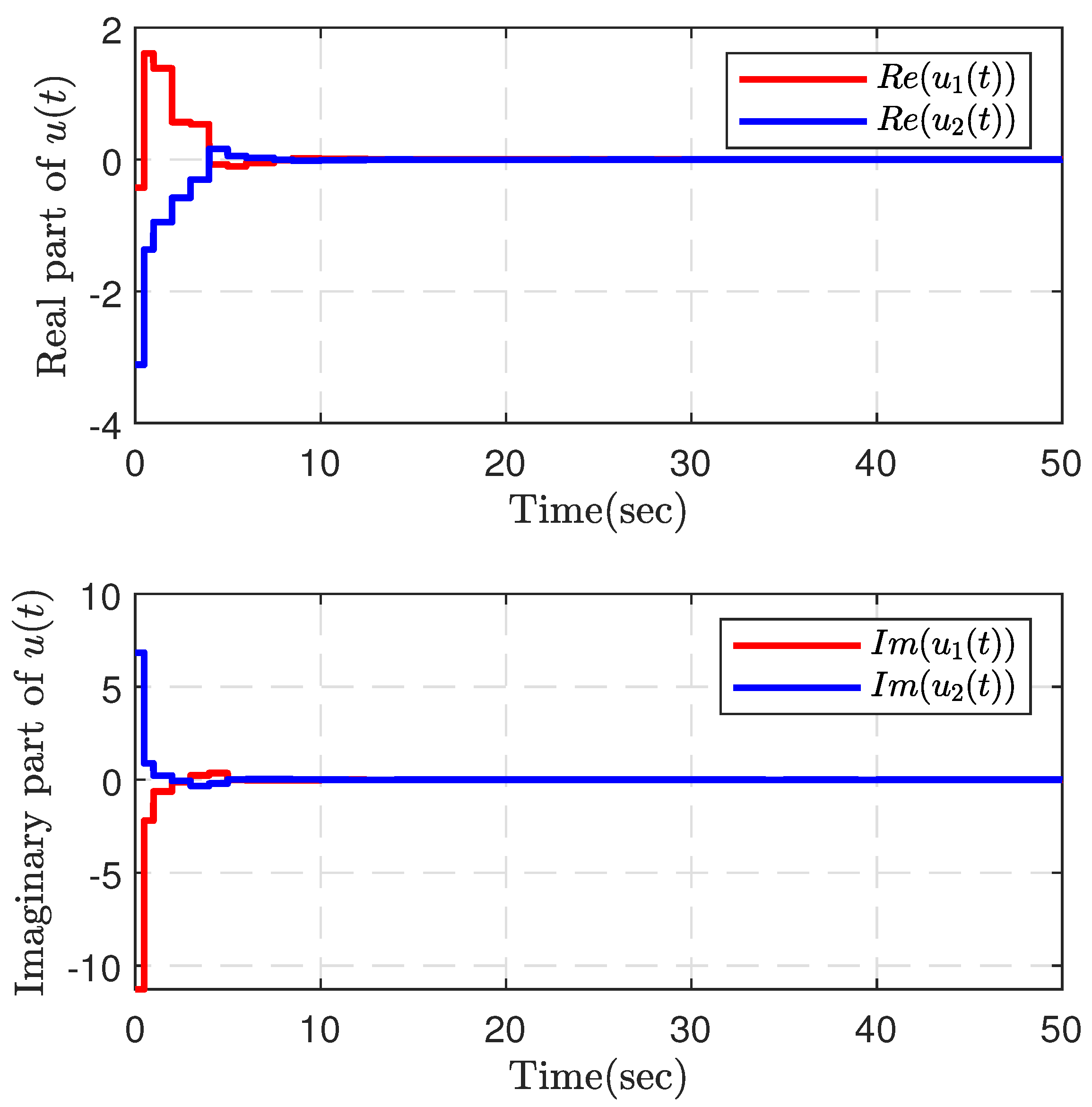
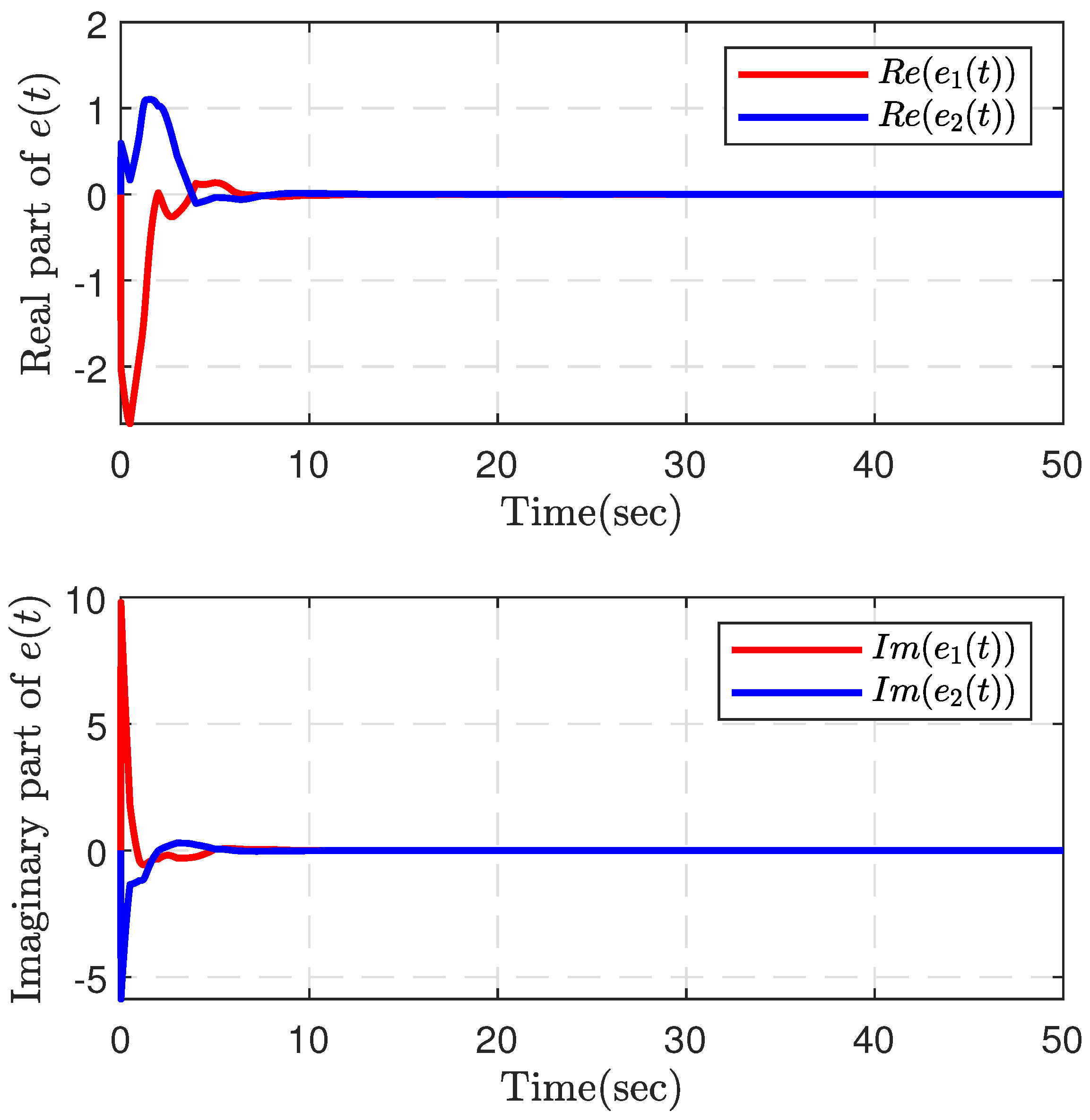
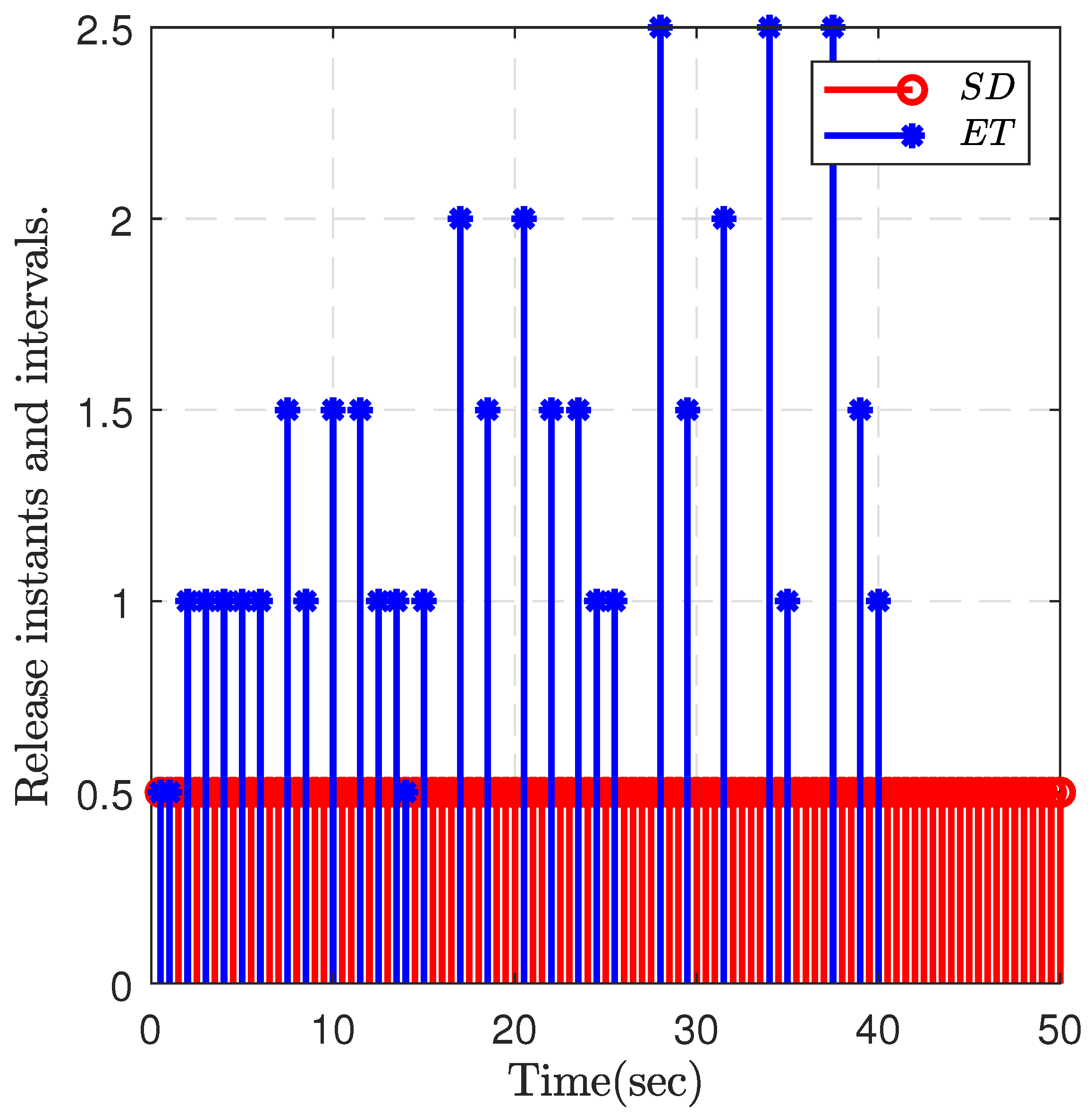
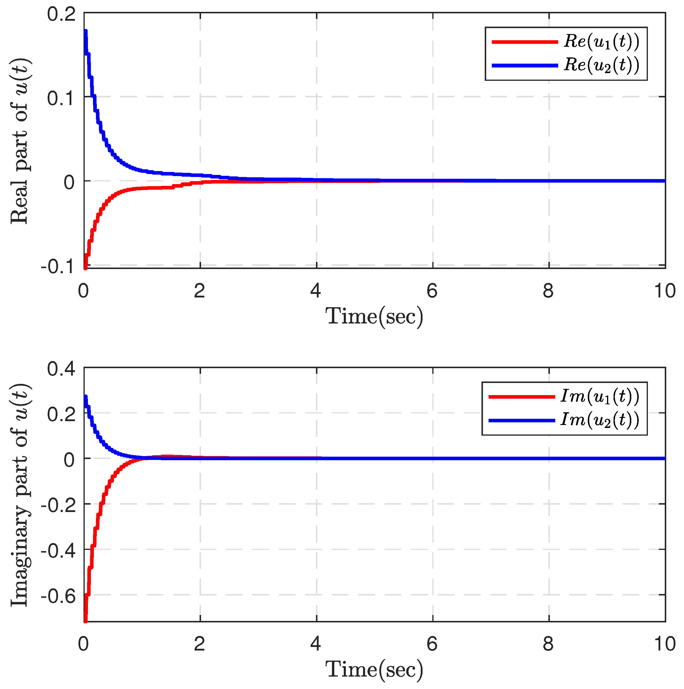
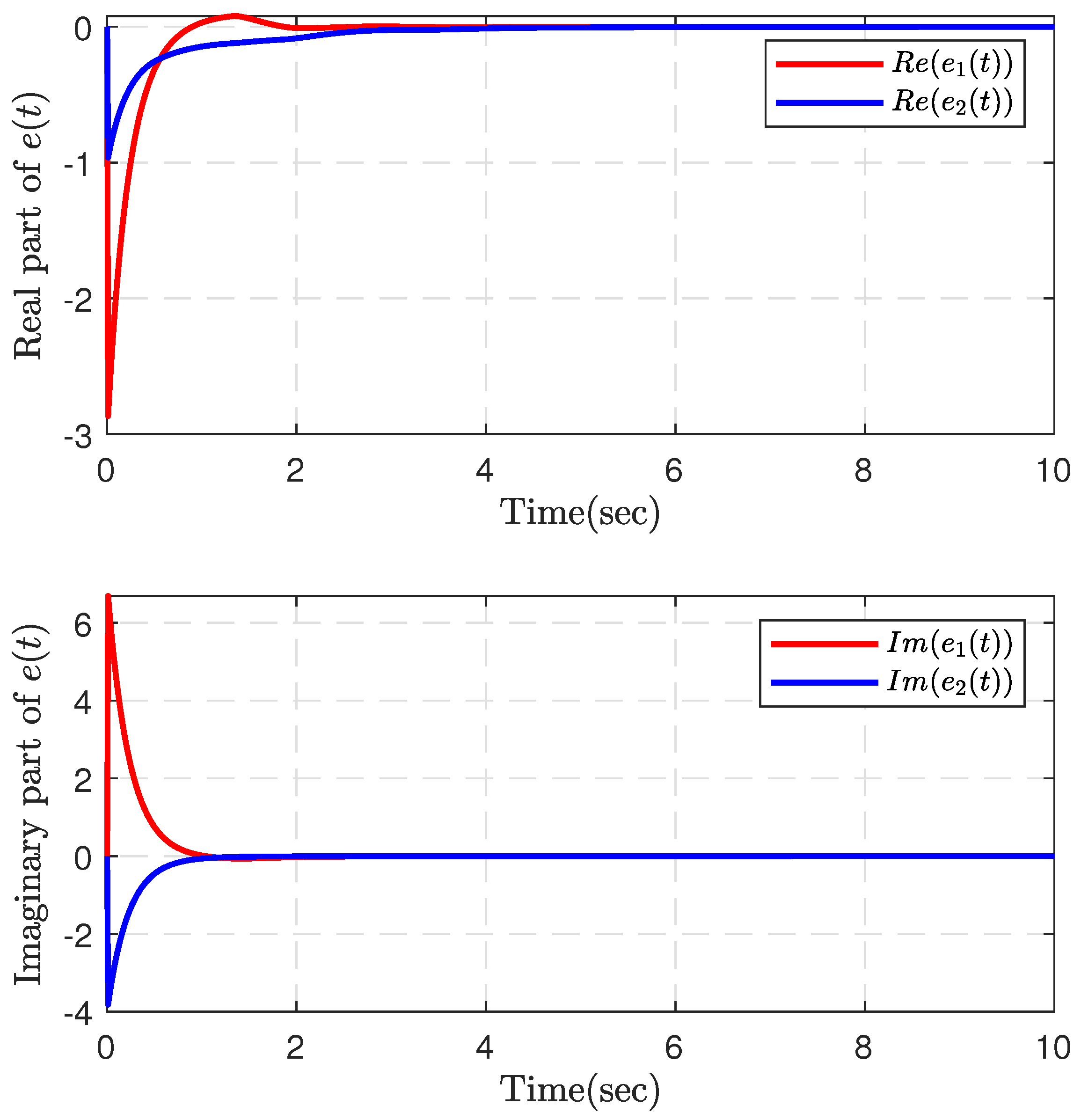
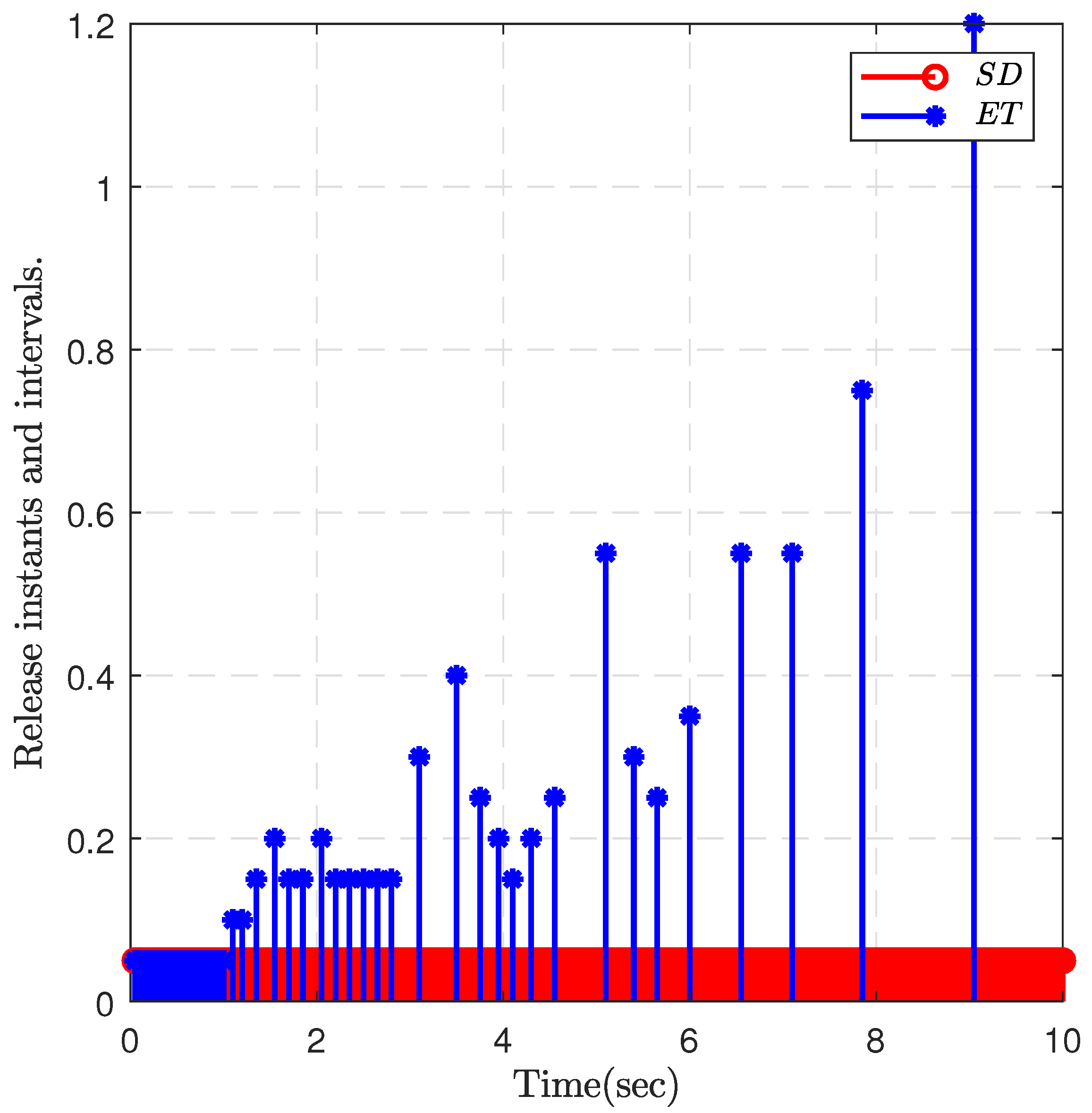
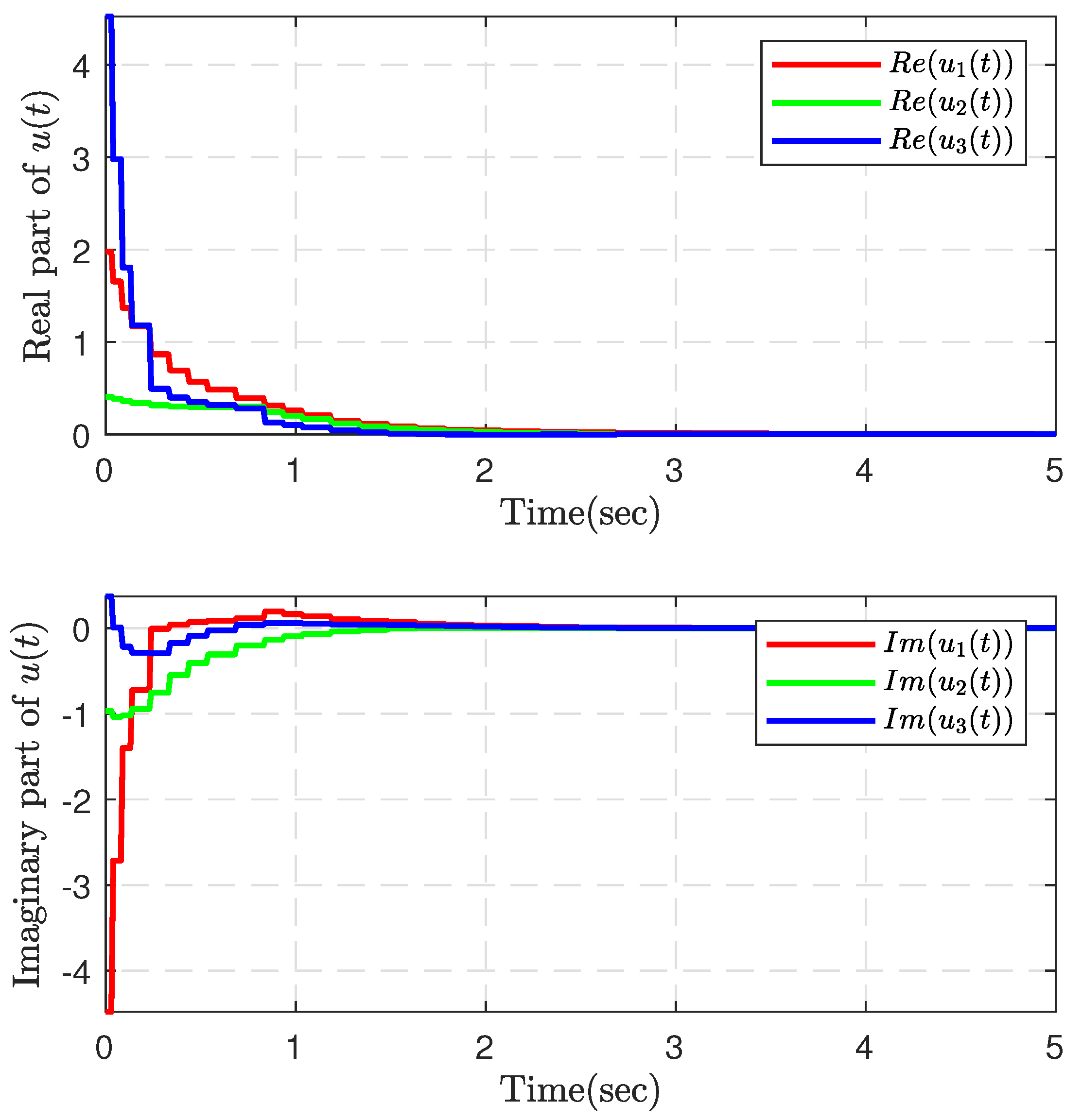
4. Numerical Examples

In this section, an illustrative numerical simulation is provided to confirm the validity of the theoretical results.

Example 1.

Consider the following FOCVNNs:

$$\begin{array}{cc}\hfill & C=diag\left\{0.94,0.92\right\},A=\left[\begin{array}{cc}0.9+0.9i& -0.9+0.8i\\ 0.8+0.4i& 0.2+0.7i\end{array}\right],B=\left[\begin{array}{cc}-0.7+0.4i& -0.5-0.6i\\ -0.6-0.5i& 0.5+0.6i\end{array}\right].\hfill \end{array}$$

The activation function satisfying condition (10) is

$$f_j\left({\mathfrak{z}}_j\left(t\right)\right)=tanh\left(Re\left({\mathfrak{z}}_j\left(t\right)\right)\right)+itanh\left(Im\left({\mathfrak{z}}_j\left(t\right)\right)\right),j=1,2.$$

Let sampling period $h=0.5$ and ${\vartheta }_1\left(t\right)=0.9\left|sin\left(0.7t\right)\right|,{\vartheta }_2\left(t\right)=0.5\left|cos\left(0.5t\right)\right|$. Some parameters are considered as $\alpha =0.99$, $L_1=diag\{1,1\}$, $L_2=diag\{0.5,0.5\}$, ${\vartheta }_1=0.9$, ${\vartheta }_2=0.5$, $\sigma =0.3$.

The control gain matrix can be computed by applying MATLAB’s LMIs toolbox to solve Theorem 1:

$$K=\left[\begin{array}{cc}-0.7607+0.0055i& 0.5707-0.3726i\\ 0.3388+0.2251i& -0.6468+0.0337i\end{array}\right].$$

In terms of Theorem 1, the FOCVNNs (16) with the SDBETM (13) are stable.

Based on these control gain matrices and $\mathfrak{z}\left(t\right)={[1-5i,-0.3+3i]}^H,$$\widehat{\mathfrak{z}}\left(t\right)={[-1+5i,0.3-3i]}^H,$ the state trajectories of the FOMs (9) and FOSs (11) are illustrated in Figure 1. It is clear that the FOMs (9) and FOSs (11) are synchronized under the proposed SDBETM. Furthermore, Figure 2 and Figure 3 depict the response information of control input $u\left(t\right)$ and error state $\mathfrak{e}\left(t\right)$ with the given controller, respectively. Figure 3 shows that the error response gradually converges to zero, which indicates that FOMs (9) and FOSs (11) are synchronous.

On the other hand, clearly depicted in Figure 4, the event-trigger frequency for the SDBETM is substantially lower than that of periodic sampling control, with the intervals between event triggers exceeding the sampling intervals. This demonstrates that the SDBETM is more efficient in conserving network resources than periodic sampling control, while also effectively preventing Zeno behavior.

From the comparison in

Table 1. Number of event triggers compared to those of other FOIIs under different $\alpha$ values (${\vartheta }_1=0.9$, ${\vartheta }_2=0.5$).

$\mathit{\alpha }$	Theorem 1	Lemma 4 in [24]	Theorem 2	Corollary 1 in [22]
$0.99$	30	31	35	39
$0.9$	18	24	29	27
$0.8$	15	18	15	16

, it is clear that the new FMBFOII generates significantly fewer event triggers across all values of α compared to other FOIIs. Meanwhile, as α increases, the corresponding number of event triggers also rises, which will increase the consumption of network resources. Similarly,

Table 2. Number of event triggers compared to those of other FOIIs under different ${\vartheta }_2$ values (${\vartheta }_1=0.9$, $\alpha =0.99$).

${\mathit{\vartheta }}_2$	Theorem 1	Lemma 4 in [24]	Theorem 2	Corollary 1 in [22]
$0.5$	30	31	35	39
$0.7$	37	39	40	45
$1.0$	40	39	46	44
$1.5$	37	38	50	46

shows that the novel FMBFOII consistently produces fewer event triggers than other FOIIs under varying ${\vartheta }_2$ values. As ${\vartheta }_2$ increases, the number of event triggers rises accordingly, leading to inefficient use of network resources.

In summary, the theoretical results derived from the novel FMBFOII consistently outperform those of other FOIIs, providing further evidence of its superiority in reducing conservatism.

Example 2.

Consider the following two-neuron FOCVNNs in [45]:

$$\begin{array}{cc}& C=\left[\begin{array}{cc}4& 0\\ 0& 4.2\end{array}\right],A=B=\left[\begin{array}{cc}1i& -1\\ 1i& 2i\end{array}\right].\hfill \end{array}$$

The activation function satisfying condition (10) is

$$\begin{array}{c}\hfill f_j\left({\mathfrak{z}}_j\left(t\right)\right)={\displaystyle \frac{1}{5}}\left(\right|Re\left({\mathfrak{z}}_j\left(t\right)\right)|+|Im\left({\mathfrak{z}}_j\left(t\right)\right)\left|i\right).\end{array}$$

Let sampling period $h=0.05$ and ${\vartheta }_1\left(t\right)=0.9\left|sin\left(0.5t\right)\right|,{\vartheta }_2\left(t\right)=0.5\left|cos\left(0.9t\right)\right|$. Some parameters are considered as $\alpha =0.99$, $L_1=diag\{1,1\}$, $L_2=diag\{0.5,0.5\}$, ${\vartheta }_1=0.9$, ${\vartheta }_2=0.5$, $\sigma =0.03$.

The control gain matrix can be computed by applying MATLAB’s LMIs toolbox to solve Theorem 1:

$$K=\left[\begin{array}{cc}-0.0711+0.0315i& 0.0353-0.0154i\\ -0.0030-0.0057i& -0.0726+0.0142i\end{array}\right].$$

In terms of Theorem 1, the FOCVNNs (16) with SDBETMs (13) are stable.

As with the analysis in Example 1, based on the control gain matrix and $\mathfrak{z}\left(t\right)={[2-5i,-1+3i]}^H,$$\widehat{\mathfrak{z}}\left(t\right)={[-1+2i,-2-1i]}^H,$ Figure 5 shows the state trajectories of the FOMs (9) and FOSs (11). Figure 6 and Figure 7 depict the response information of control input $u\left(t\right)$ and error state $\mathfrak{e}\left(t\right)$ with the given event-trigger controller, respectively. The release instants and release intervals of the SDBETM are shown in Figure 8.

Example 3.

Consider the following 3-D FOCVNNs in [46]:

$$\begin{array}{cc}\hfill C& =diag\left\{0.8,0.8,0.8\right\},\hfill \\ \hfill A& =\left.\left[\begin{array}{ccc}2.2-1.7i& -1-0.1i& -0.1+0.1i\\ -1.3+1.8i& 0.7-0.2i& -0.5+0.2i\\ -1.4-1.9i& 0.8+0.2i& -0.3-0.2i\end{array}\right.\right],\hfill \\ \hfill B& =\left.\left[\begin{array}{ccc}1.2+1.5i& -0.7+0.2i& -0.3+0.4i\\ 1.3+1.7i& 0.6-0.3i& -0.4+0.5i\\ 1.2+1.6i& 0.9+0.1i& -0.3+0.2i\end{array}\right.\right].\hfill \end{array}$$

The activation functions are chosen as

$$\begin{array}{c}\hfill f_j\left({\mathfrak{z}}_j\left(t\right)\right)=0.2tanh\left(Re\left({\mathfrak{z}}_j\left(t\right)\right)\right)+i·0.2tanh\left(Im\left({\mathfrak{z}}_j\left(t\right)\right)\right).\end{array}$$

Let sampling period $h=0.05$ and ${\vartheta }_1\left(t\right)=0.9\left|sin\left(0.5t\right)\right|,{\vartheta }_2\left(t\right)=0.5\left|cos\left(0.9t\right)\right|$. Some parameters are considered as $\alpha =0.99$, $L_1=diag\{1,1,1\}$, $L_2=diag\{0.5,0.5,0.5\}$, ${\vartheta }_1=0.9$, ${\vartheta }_2=0.5$, $\sigma =0.03$.

The following control gain is obtained by using MATLAB’s LMIs toolbox:

$$K=\left[\begin{array}{ccc}-5.8119-0.0655i& 0.9530+3.6909i& 0.6560-0.8400i\\ 0.8910-3.8708i& -4.5700+0.1700i& -0.8632+0.1788i\\ 0.7577+0.6476i& -0.9440-0.3418i& -1.4688-0.1096i\end{array}\right].$$

Therefore, the FOMs (9) and FOSs (11) are synchronous. Figure 9 represents the state response of all the trajectories of the FOMs (9) and FOSs (11) with the initial conditions $\mathfrak{z}\left(t\right)={[0.4-0.3i,0.3-0.3i,0.2-0.2i]}^T,$$\widehat{\mathfrak{z}}\left(t\right)={[-0.4+0.3i,-0.3+0.3i,-0.2+0.2i]}^H.$ Figure 10 and Figure 11 depict the response information of control input $u\left(t\right)$ and error state $\mathfrak{e}\left(t\right)$ with the given event-trigger controller, respectively. Figure 12 shows release instants and release intervals of the SDBETM (13).

Combining the contents of the above several figures, it is easy to verify the correctness and validity of the theoretical results of this research.

5. Conclusions

In the present treatise, the synchronization control issue for FOCVNNs with additive TVDs has been investigated utilizing the SDBETM. A new FMBFOII has been proposed and a novel FOCVII containing FDs, TVDs, and triggering instants has been constructed. In addition, to reduce network transmission and save network resources, the SDBETM has been introduced. A new LKF containing more information about additive TVDs and triggering instants has been constructed. Then, based on the modified FOCVII, WBFOII, and LKF, and combined with the SDBETM, two less conservative and sufficient conditions guaranteeing that the FOCVNNs with additive TVDs are asymptotically stable have been obtained. Ultimately, numerical simulations have been provided to confirm the effectiveness of the theoretical outcomes. In future endeavors, the results of this research can be utilized to analyze and synthesize FOCVNNs with Markovian jump parameters and ATVDs, as well as for robust control design and cost control.

References

1. Kiruthika, R.; Krishnasamy, R.; Lakshmanan, S.; Prakash, M.; Manivannan, A. Non-fragile sampled-data control for synchronization of chaotic fractional-order delayed neural networks via LMI approach. Chaos Solitons Fractals 2023, 169, 113252. [Google Scholar] [CrossRef]
2. Mukdasai, K. Synchronization of Fractional-Order Uncertain Delayed Neural Networks with an Event-Triggered Communication Scheme. Fractal Fract. 2022, 6, 641. [Google Scholar] [CrossRef]
3. Bao, H.; Cao, J.; Kurths, J. State estimation of fractional-order delayed memristive neural networks. Nonlinear Dyn. 2018, 94, 1215–1225. [Google Scholar] [CrossRef]
4. Padmaja, N.; Balasubramaniam, P. Design of H/passive state feedback control for delayed fractional order gene regulatory networks via new improved integral inequalities. Commun. Nonlinear Sci. Numer. Simul. 2022, 111, 106507. [Google Scholar] [CrossRef]
5. Liang, J.; Li, K.; Song, Q.; Zhao, Z.; Liu, Y.; Alsaadi, F.E. State estimation of complex-valued neural networks with two additive time-varying delays. Neurocomputing 2018, 309, 54–61. [Google Scholar] [CrossRef]
6. Wei, X.; Zhang, Z.; Lin, C.; Chen, J. Synchronization and anti-synchronization for complex-valued inertial neural networks with time-varying delays. Appl. Math. Comput. 2021, 403, 126194. [Google Scholar] [CrossRef]
7. Pan, J.; Zhang, Z. Finite-time synchronization for delayed complex-valued neural networks via the exponential-type controllers of time variable. Chaos Solitons Fractals Appl. Sci. Eng. Interdiscip. J. Nonlinear Sci. 2021, 146, 110897. [Google Scholar] [CrossRef]
8. Subramanian, K.; Muthukumar, P. Global asymptotic stability of complex-valued neural networks with additive time-varying delays. Cogn. Neurodynamics 2017, 11, 293–306. [Google Scholar] [CrossRef]
9. Yao, L.; Wang, Z.; Wang, Q.; Xia, J.; Shen, H. Exponential Stabilization of Delayed Complex-valued Neural Networks with Aperiodic Sampling: A Free-matrix-based Time-dependent Lyapunov Functional Method. Int. J. Control Autom. Syst. 2020, 18, 1894–1903. [Google Scholar] [CrossRef]
10. Aghayan, Z.S.; Alfi, A.; Mousavi, Y.; Fekih, A. Stability analysis of a class of variable fractional-order uncertain neutral-type systems with time-varying delay. J. Frankl. Inst. 2023, 360, 10517–10535. [Google Scholar] [CrossRef]
11. Aghayan, Z.S.; Alfi, A.; Mousavi, Y.; Kucukdemiral, I.B.; Fekih, A. Guaranteed cost robust output feedback control design for fractional-order uncertain neutral delay systems. Chaos Solitons Fractals 2022, 163, 112523. [Google Scholar] [CrossRef]
12. Aghayan, Z.S.; Alfi, A.; Mousavi, Y.; Fekih, A. Criteria for stability and stabilization of variable fractional-order uncertain neutral systems with time-varying delay: Delay-dependent analysis. IEEE Trans. Circuits Syst. II Express Briefs 2023, 70, 3393–3397. [Google Scholar] [CrossRef]
13. Xiong, M.; Ju, G.; Tan, Y. Robust State Estimation for Fractional-Order Nonlinear Uncertain Systems via Adaptive Event-Triggered Communication Scheme. IEEE Access 2019, 7, 115002–115009. [Google Scholar] [CrossRef]
14. Chen, S.; Song, Q.; Zhao, Z.; Liu, Y.; Alsaadi, F.E. Global asymptotic stability of fractional-order complex-valued neural networks with probabilistic time-varying delays. Neurocomputing 2021, 450, 311–318. [Google Scholar] [CrossRef]
15. Aravind, R.V.; Balasubramaniam, P. Stochastic stability of fractional-order Markovian jumping complex-valued neural networks with time-varying delays. Neurocomputing 2021, 439, 122–133. [Google Scholar] [CrossRef]
16. Zhang, H.; Qiu, Z.; Xiong, L. Stochastic stability criterion of neutral-type neural networks with additive time-varying delay and uncertain semi-Markov jump. Neurocomputing 2019, 333, 395–406. [Google Scholar] [CrossRef]
17. Cao, Y.; Sriraman, R.; Shyamsundarraj, N.; Samidurai, R. Robust stability of uncertain stochastic complex-valued neural networks with additive time-varying delays. Math. Comput. Simul. 2020, 171, 207–220. [Google Scholar] [CrossRef]
18. Felipe, A.; Oliveira, R.C. An LMI-based algorithm to compute robust stabilizing feedback gains directly as optimization variables. IEEE Trans. Autom. Control 2020, 66, 4365–4370. [Google Scholar] [CrossRef]
19. Nguyen, T.H.; Nguyen, V.C.; Bui, D.Q.; Dao, P.N. An efficient Min/Max Robust Model Predictive Control for nonlinear discrete-time systems with dynamic disturbance. Chaos Solitons Fractals 2024, 180, 114551. [Google Scholar] [CrossRef]
20. Seuret, A.; Gouaisbaut, F. Jensen’s and Wirtinger’s inequalities for time-delay systems. IFAC Proc. Vol. 2013, 46, 343–348. [Google Scholar] [CrossRef]
21. Zeng, H.B.; He, Y.; Wu, M.; She, J. Free-matrix-based integral inequality for stability analysis of systems with time-varying delay. IEEE Trans. Autom. Control 2015, 60, 2768–2772. [Google Scholar] [CrossRef]
22. Hu, T.; He, Z.; Zhang, X.; Zhong, S. Leader-following consensus of fractional-order multi-agent systems based on event-triggered control. Nonlinear Dyn. 2020, 99, 2219–2232. [Google Scholar] [CrossRef]
23. Hu, T.; He, Z.; Zhang, X.; Zhong, S. Global synchronization of time-invariant uncertainty fractional-order neural networks with time delay. Neurocomputing 2019, 339, 45–58. [Google Scholar] [CrossRef]
24. Hu, T.; Park, J.H.; Liu, X.; He, Z.; Zhong, S. Sampled-data-based event-triggered synchronization strategy for fractional and impulsive complex networks with switching topologies and time-varying delay. IEEE Trans. Syst. Man, Cybern. Syst. 2021, 52, 3568–3580. [Google Scholar] [CrossRef]
25. Wen, G.; Chen, M.Z.; Yu, X. Event-triggered master–slave synchronization with sampled-data communication. IEEE Trans. Circuits Syst. II Express Briefs 2015, 63, 304–308. [Google Scholar] [CrossRef]
26. Zhou, L.; Liu, C.; Pan, R.; Xiao, X. Event-triggered synchronization of switched nonlinear system based on sampled measurements. IEEE Trans. Cybern. 2020, 52, 3531–3538. [Google Scholar] [CrossRef] [PubMed]
27. Guan, C.; Sun, D.; Fei, Z.; Ren, C. Synchronization for switched neural networks via variable sampled-data control method. Neurocomputing 2018, 311, 325–332. [Google Scholar] [CrossRef]
28. Li, H.; Li, C.; Ouyang, D.; Nguang, S.K. Impulsive synchronization of unbounded delayed inertial neural networks with actuator saturation and sampled-data control and its application to image encryption. IEEE Trans. Neural Netw. Learn. Syst. 2020, 32, 1460–1473. [Google Scholar] [CrossRef]
29. Xiao, L.; Li, L.; Cao, P.; He, Y. A fixed-time robust controller based on zeroing neural network for generalized projective synchronization of chaotic systems. Chaos Solitons Fractals 2023, 169, 113279. [Google Scholar] [CrossRef]
30. Li, H.L.; Hu, C.; Cao, J.; Jiang, H.; Alsaedi, A. Quasi-projective and complete synchronization of fractional-order complex-valued neural networks with time delays. Neural Netw. 2019, 118, 102–109. [Google Scholar] [CrossRef]
31. Liu, D.; Zhu, S.; Sun, K. Global anti-synchronization of complex-valued memristive neural networks with time delays. IEEE Trans. Cybern. 2018, 49, 1735–1747. [Google Scholar] [CrossRef] [PubMed]
32. Xu, B.; Li, B. Event-Triggered State Estimation for Fractional-Order Neural Networks. Mathematics 2022, 10, 325. [Google Scholar] [CrossRef]
33. Xing, X.; Wu, H.; Cao, J. Event-triggered impulsive control for synchronization in finite time of fractional-order reaction–diffusion complex networks. Neurocomputing 2023, 557, 126703. [Google Scholar] [CrossRef]
34. Yu, N.; Zhu, W. Exponential stabilization of fractional-order continuous-time dynamic systems via event-triggered impulsive control. Nonlinear Anal. Model. Control 2022, 27, 592–608. [Google Scholar] [CrossRef]
35. Liu, F.; Yang, Y.; Wang, F.; Zhang, L. Synchronization of fractional-order reaction–diffusion neural networks with Markov parameter jumping: Asynchronous boundary quantization control. Chaos Solitons Fractals 2023, 173, 113622. [Google Scholar] [CrossRef]
36. Sun, Y.; Hu, C.; Yu, J.; Shi, T. Synchronization of fractional-order reaction-diffusion neural networks via mixed boundary control. Appl. Math. Comput. 2023, 450, 127982. [Google Scholar] [CrossRef]
37. Fan, Q.Y.; Yang, G.H. Sampled-data output feedback control based on a new event-triggered control scheme. Inf. Sci. 2017, 414, 306–318. [Google Scholar] [CrossRef]
38. Peng, C.; Han, Q.L. A Novel Event-Triggered Transmission Scheme and L_2 Control Co-Design for Sampled-Data Control Systems. IEEE Trans. Autom. Control 2013, 58, 2620–2626. [Google Scholar] [CrossRef]
39. Yang, Y.; Tu, Z.; Wang, L.; Cao, J.; Shi, L.; Qian, W. H infinity synchronization of delayed neural networks via event-triggered dynamic output control. Neural Netw. 2021, 142, 231–237. [Google Scholar] [CrossRef]
40. Qiu, Q.; Su, H. Sampling-based event-triggered exponential synchronization for reaction-diffusion neural networks. IEEE Trans. Neural Netw. Learn. Syst. 2021, 34, 1209–1217. [Google Scholar] [CrossRef]
41. Zhao, L.N.; Ma, H.J.; Xu, L.X.; Wang, X. Observer-based adaptive sampled-data event-triggered distributed control for multi-agent systems. IEEE Trans. Circuits Syst. II Express Briefs 2019, 67, 97–101. [Google Scholar] [CrossRef]
42. Hu, T.; He, Z.; Zhang, X.; Zhong, S. Finite-time stability for fractional-order complex-valued neural networks with time delay. Appl. Math. Comput. 2020, 365, 124715. [Google Scholar] [CrossRef]
43. Hu, T.; He, Z.; Zhang, X.; Zhong, S.; Yao, X. New fractional-order integral inequalities: Application to fractional-order systems with time-varying delay. J. Frankl. Inst. 2021, 358, 3847–3867. [Google Scholar] [CrossRef]
44. Padmaja, N.; Balasubramaniam, P. Results on passivity analysis of delayed fractional-order neural networks subject to periodic impulses via refined integral inequalities. Comput. Appl. Math. 2022, 41, 136. [Google Scholar] [CrossRef]
45. Gunasekaran, N.; Zhai, G. Sampled-data state-estimation of delayed complex-valued neural networks. Int. J. Syst. Sci. 2020, 51, 303–312. [Google Scholar] [CrossRef]
46. Wang, X.; Wang, Z.; Song, Q.; Shen, H.; Huang, X. A waiting-time-based event-triggered scheme for stabilization of complex-valued neural networks. Neural Netw. 2020, 121, 329–338. [Google Scholar] [CrossRef] [PubMed]
Figure 1. State trajectories of FOMs z ( t ) and FOSs z ^ ( t ) ( x = z , y = z ^ ).
Fractalfract 08 00569 g001
Figure 2. Control input u(t).
Fractalfract 08 00569 g002
Figure 3. State trajectories of error e ( t ) ( e = e ).
Fractalfract 08 00569 g003
Figure 4. The event-triggered and sampled release instants and intervals.
Fractalfract 08 00569 g004
Figure 5. State trajectories of FOMs z ( t ) and FOSs z ^ ( t ) ( x = z , y = z ^ ).
Fractalfract 08 00569 g005
Figure 6. Control input u(t).
Fractalfract 08 00569 g006
Figure 7. State trajectories of error e ( t ) ( e = e ).
Fractalfract 08 00569 g007
Figure 8. The event-triggered and sampled release instants and intervals.
Fractalfract 08 00569 g008
Figure 9. State trajectories of FOMs z ( t ) and FOSs z ^ ( t ) ( x = z , y = z ^ ).
Fractalfract 08 00569 g009
Figure 10. Control input u(t).
Fractalfract 08 00569 g010
Figure 11. State trajectories of error e ( t ) ( e = e ).
Fractalfract 08 00569 g011
Figure 12. The event-triggered and sampled release instants and intervals.
Fractalfract 08 00569 g012