The Spatial Variation of Soil Structure Fractal Derived from Particle Size Distributions at the Basin Scale

Abstract

The accurate characterization of soil structure is fundamental to groundwater science, environmental ecology, and Earth systems science. To address the challenge of quantifying the high spatial variability of large-scale soil structures, this study used a laser particle size analyzer to measure the distribution of soil particle size in 207 samples from ten profiles across the Daqing and Ziya River basins in the North China Plain. The quantified soil structure, expressed as soil fractal dimension D, was derived using monofractal theory. Various spatial analysis techniques, including Moran’s I index, correlation analysis heat maps, the Kolmogorov–Smirnov one-sample test, and geostatistical semivariogram function, were jointly applied to investigate the spatial variability of soil structural fractals across different depths in the piedmont plain–coastal areas of the two river basins. The results indicate the following: (1) Quantitative analysis confirms that under the influence of piedmont alluvial and fluvial dynamics, soil D values homogenize from the piedmont to the coastal areas, with decreasing particle size differences closer to the coast. However, the spatial variability of the soil structural fractals in the Ziya River Basin was greater than that in the Daqing River Basin. (2) The combined effects of climate change, regional differences, and human activity led to greater spatial variability in the soil structural fractals in the Ziya River Basin than in the Daqing River Basin. The correlation between D values and burial depth was strongest in the Xianxian profile (−0.78), whereas the spatial correlation was strongest in the Hengshui and Dacheng profiles (−0.47). (3) The greatest spatial variability in soil D values occurred at depths of 1–2 m, with a coefficient of variation of 23.595%, which was significantly higher than those at depths of 0–1 (14.569%) and 2–3 m (16.284%).

1. Introduction

Quantifying soil structure is important for understanding the mechanisms of surface Earth system dynamics and ecological processes [1]. This is because the soil structure fundamentally determines the key parameters of the surface system, influencing other soil properties [2], including the vadose zone hydrodynamic characteristics, solute transport behavior, and thermodynamic properties, and controlling the transformation and transport of matter and energy in saturated and unsaturated zones. Xie et al. [3] integrated global daily runoff observations from 15,500 basins and found that soil structure was the primary factor affecting the spatiotemporal variability of basin groundwater base flow indices in the Earth system model. The accurate quantification of soil structure and spatial variability at the basin scale has become fundamental in groundwater science, ecology, and Earth systems science. However, the distribution of soil particles at regional or basin scales is exceptionally complex, making it extremely difficult to accurately characterize and analyze soil structure under these conditions. This is because of the high spatial variability of the soil structure within the basins, which is influenced by sedimentation processes under perennial river erosion as material moves from the piedmont through plains to coastal areas and eventually into the sea, as seen in the major basins in the North China Plain, where intense climate change and human activity have a combined impact [4].

The North China Plain is a typical alluvial plain with a low elevation, mostly below 50 m. Since the Quaternary period, the river geological process has resulted in the accumulation of layers that are several kilometers thick, comprising various types of deposits, including alluvial, fluvial, lacustrine, and marine sediments. These diverse sediment types reflect the paleogeographic evolution of the Haihe Plain since the Quaternary, resulting in a complex and variable present-day hydrogeological environment [5]. The complex soil–water environment determines the evolution of hydraulic properties and salt migration patterns. For example, the soil permeability coefficient decreases with the depth of the alluvial plain, and the sensitivity to stratum pressure decreases from the piedmont to the coastal area [6]. The chemical composition of the groundwater exhibits an upward trend from the inclined piedmont–colluvial plain to the central alluvial–lacustrine plain and then to the coastal alluvial–marine plain. Groundwater hydrodynamic conditions deteriorate from the piedmont to the coastal area, with a gradual increase in the concentration of high salinity ions and the accumulation of soluble salts, leading to a general salinization of the water body [7]. However, before quantifying the soil structure and spatial distribution characteristics, these trends can only be expressed qualitatively, severely limiting the possibility of studying large-scale soil hydrodynamic characteristics and solute transport patterns at the regional or basin scale.

The key to quantifying the spatial expression of the soil structure depends on accurately describing the complex pore topology and spatial distribution patterns of particle size distributions (PSDs) [8]. Researchers have developed topological models for studying pore size, arrangement, and combination, leading to a series of quantitative studies on soil structure and spatial variability [9,10]. Studies have shown that the soil PSD fractal parameters determined by fractal theory exhibit a strong spatial structure [11]. Soil fractal dimensions not only characterize the size composition of soil particles but also describe the distribution of the particle sizes and pores, reflecting the uniformity of texture [12]. Additionally, using the concept of fractals and the overall surface roughness characterized by fractal dimensions to study the spatial variation in soil properties [13] can effectively quantify the spatial variability and scale effects of the soil structure [14]. In recent years, the fractional plasticity theory has made significant progress in quantifying soil rheological properties. This theory offers a novel approach to studying the plastic behavior of complex materials, enabling the accurate description of deformation characteristics under varying stress conditions through fractional-order derivatives [15,16]. Given the complex spatial distribution of soil particles and the topological structure of pores, the fractional plasticity model helps to reveal the mechanical behavior and deformation mechanisms of soils under different hydraulic conditions. This provides an important theoretical foundation for further understanding large-scale soil structures and their spatial variability. These findings provide scientific support for further studies on the other physical and chemical properties of soil and their significant roles in geological environmental changes [17].

Therefore, this study characterized the soil PSD at different depths within typical basin profiles, quantifying the soil structure using fractal theory, that is, the soil structural fractal dimension (D). Combined with spatial analysis techniques, this study was conducted in two typical basins of the North China Plain (Daqing River and Ziya River basins) to quantify the spatial variability of soil structural fractals at various depths and scales from the piedmont to the plain and coastal areas.

2. Materials and Methods

2.1. Study Area Selection

Although the Daqing and Ziya rivers flow through significantly different regions of the North China Plain, they share common characteristics, such as a thick vadose zone, typical climatic and geomorphological features, and significant spatial variability in the shallow aquifer soil structure. Both river basins consist of a piedmont alluvial fan subsystem, central ancient river channel subsystem, and an eastern coastal subsystem. Both eventually drain into the sea via the Tianjin Binhai New Area. Therefore, these two river basins were selected as typical study areas to explore the differences in soil structure spatial variability from the piedmont to the central plain and coastal areas across different basins, as well as the reasons for these differences.

The Daqing River is formed by the confluence of the Baigou and South Juma rivers in Baigou Town, Hebei, China. Its main tributaries include the Pu, Cao, Fu, Tang, and Zhulong rivers, all of which flow into Baiyangdian and then into the Bohai Sea through Tianjin, China. Based on the distribution of basin subsystems, five typical profiles were selected for the Daqing River basin: the Shijiazhuang profile on the southern edge of the Daqing River basin in the piedmont plain (with a thick vadose zone and groundwater levels between 28–45 m); the Wangdu, Anxin, and Baiyangdian profiles in the river confluence area in the central plain (with significant lithological differences); and the Tianjin profile in the coastal area.

The Ziya River Basin (Figure 1) is located between the Daqing River and the Zhangwei South Canal in the southern part of the Haihe River Basin, China. It consists of two major tributaries, the Fuyang and Hutuo rivers. These two river systems converge in Xian County and flow into the Bohai Sea via the Ziya New River. Based on the distribution of basin subsystems, five profiles were selected within the basin: the Luancheng profile in the piedmont plain (with a thick vadose zone and groundwater levels between 33–43 m); the Hengshui, Xian County, and Hejian profiles in the central plain; and the Dacheng profile in the coastal area.

Thus, ten profiles were selected for the study area (

Table 1. Geographic characteristics of the sampling sites.

Sample Num.	Depth (m)	Location	District	Geographical Coordinates		Elevation (m)
				ψ (N)	λ (E)
SJZ01-30	0–3.0	Shijiazhuang City	The western piedmont	114°40′33″	37°53′16″	85
LC01-26	0–3.0	Luancheng County, Shijiazhuang City		114°28′58″	38°04′59″	55
WD01-04	0.9–1.3	Wangdu County, Baoding City	The median plain	115°09′18″	38°24′40″	46
AX01-06	0.4–1.2	laohetou Town, Anxin County		115°41′55″	38°30′24″	13
BYL01-09	0.4–1.6	Baiyang Lake, Anxin County		116°03′10″	38°35′52″	5
HS01-25	0–2.5	Shenzhou County, Hengshui City		115°30′58″	38°27′14″	30
XX01-19	0–1.9	Xianxian County, Cangzhou City		116°10′11″	38°29′29″	15
HJ01-23	0–2.3	Hejian County, Cangzhou City		116°07′55″	38°32′53″	14
DC01-30	0–3.0	Dacheng County, Langfang City	Eastern coastal areas	116°38′20″	38°39′37″	8
BH01-11	0–1.1	Binhai new-region, Tianjin City		117°32′24″	39°00′48″	4

), with sampling lines forming a triangular layout on the map. The piedmont plain converges in Shijiazhuang, and the coastal area converges in Tianjin (Figure 1).

2.2. Test Arrangement

Based on previous lithological and grain-size analysis data for typical profiles, sampling points were determined for the piedmont, central plain, and coastal regions. For the Shijiazhuang and Luancheng profiles, samples were taken between 0.3–24.6 m, with a total of 38 samples collected. The Wangdu, Anxin, Baiyangdian profiles are typical of plain areas in the Daqing River Basin, with samples taken from 0.4–1.6 m, totaling 19 samples. The profiles of Hengshui, Xian County, and Hejian represent the plain region of the Ziya River Basin, with samples taken from 0.1–3.0 m, totaling 90 samples. The Dacheng and Tianjin profiles are coastal, with samples taken from 0.1–3.0 m, totaling 60 samples. A total of 207 samples were collected from the ten profiles.

From west to east, the horizontal distances from the Wangdu profile to the Anxin, Baiyangdian, and Tianjin profiles were 73, 32, and 90 km, respectively, forming a piedmont–coastal sampling line for the Daqing River basin.

From north to south, the vertical distances from the Anxin profile to the Baiyangdian, Hejian, Xian County, and Hengshui profiles were 15, 51, 80, and 115 km, respectively, forming the central plain sampling line.

From north to south, the vertical distance between the Dacheng and Tianjin profiles is 32 km, forming a coastal area sampling line.

From west to east, the horizontal distances from the Shijiazhuang profile to the Luancheng, Wangdu, Hengshui, Anxin, Xian County, Baiyangdian, Hejian, Dacheng, and Tianjin profiles were 15, 60, 94, 133, 145, 165, 178, 202, and 258 km, respectively, forming a piedmont–central plain–coastal area sampling line across the North China Plain.

2.3. Sample Testing and Fractal Dimension Theory

Each sample group comprised three parts that were thoroughly mixed. The particle size volume percentages of the soil samples were determined using a Master Sizer 2000 laser particle size analyzer (Malvern Instruments, Malvern, UK). A total of 130 particle size intervals, ranging from 0 to 2000 μm, were tested for their volume percentages and cumulative percentages. The fractal dimensions (D) of the 207 samples were calculated using fractal theory. The specific theoretical applications are as follows.

The fractal calculation of the soil particle size was based on the fractal model of the volume distribution across different particle sizes, which can be expressed as the following:

$${\left[{\displaystyle \frac{d_i}{d_{max}}}\right]}^{\left(3-D\right)}={\displaystyle \frac{V(\delta <d_i)}{V_0}}$$

(1)

where d_i (i = 1, 2, 3, …, n) represents the diameter of soil particles, d_max is the maximum diameter of soil particles, D is the fractal dimension, δ is the variable soil particle size, V (δ < d_i) is the volume of soil particles with diameters smaller than d_i, and V₀ is the volume of the soil sample [12].

When calculating the fractal dimension, we first calculated $\mathit{lg}{\displaystyle \frac{V(\delta <d_i)}{V_0}}$ and $\mathit{lg}{\displaystyle \frac{d_i}{d_{max}}}$ from the measured particle sizes and their corresponding volumes. Then $\mathit{lg}{\displaystyle \frac{V(\delta <d_i)}{V_0}}$ was plotted on the vertical axis and $\mathit{lg}{\displaystyle \frac{d_i}{d_{max}}}$ on the horizontal axis, and the least squares method was used to fit a straight line to these data points, determining the slope. Finally, fractal dimension D of the sample was calculated.

2.4. Theories and Methods of Spatial Variation Analysis

2.4.1. Spatial Autocorrelation

In this study, the global Moran’s I index [19] was used to demonstrate the spatial dependence (autocorrelation) of the fractal dimensions across each soil profile. The formula is as follows:

$$Mora{n}^{\prime }sI=n{\sum }_{i=1}^n{\sum }_{j=1}^n{\displaystyle \frac{W_i\left(x_i-\overline{x}\right)\left(x_i-\overline{x}\right)}{\sum _{i=1}\sum _{i=1}^n{W}_i\sum _{i=1}^n{\left(x_i-x\right)}^2}}$$

(2)

where n represents the number of sample points to be estimated; x_i and x_j are the observed values of variable x at sample points i and j, respectively; $\overline{x}$ is the mean value of x; and W_ij is the neighboring weight. The range of values of I is [−1, 1]; when I = 0, the variable has no spatial correlation and is randomly distributed. When I tends to 1, the spatial distribution of the variables shows a completely positive correlation and clustering. When I tends to −1, the variables exhibit a completely negative correlation and scattered distribution.

2.4.2. Normality Test

The Kolmogorov–Smirnov (K-S) test is a nonparametric statistical test used to determine whether a sample conforms to a particular probability distribution [20]. It can be divided into one-sample K-S tests (to assess whether a single sample comes from a particular probability distribution) and two-sample K-S tests (to assess whether two samples come from the same probability distribution). In this study, a one-sample K-S test was used to test the normality of fractal dimension D for soil samples at a confidence level of 5%. The conclusion was drawn based on the p-values.

2.4.3. Spatial Heterogeneity

This study used a semivariogram function from geostatistics [21] to analyze and describe the spatial distribution, variability, and correlation characteristics of soil fractal dimensions. The sample semivariogram function, γ(h), effectively reflects the influence of random factors on the soil fractal dimension and its spatial correlation relationships. The sample semivariogram function can be expressed as the following:

$$\gamma \left(h\right)={\displaystyle \frac{1}{2N_h}}{\sum }_{i=1}^n{\left[Z\left(x_i+h\right)-Z\left(x_i\right)\right]}^2$$

(3)

where γ(h) represents the sample semivariance function value, Z(x_i) denotes the sample data series, and N_h is the number of sample pairs used to estimate the semivariance function value. In this study, geostatistical software GS+ 9.0 was used to analyze the semivariance functions of the soil fractal D values. Anisotropic semivariance functions were fitted using spherical, exponential, Gaussian, and linear models. The optimal theoretical model was chosen based on the criteria of a higher determination coefficient (R²) and lower residual sum of squares (RSS), as well as considering the range and nugget effects. This optimal model was then used for the Kriging interpolation.

2.4.4. Kriging Interpolation

Kriging interpolation is a regression algorithm based on a covariance function for the spatial modeling and prediction of random processes or random fields. This method is commonly used for spatial interpolations in geostatistics. Kriging interpolation includes several algorithms, such as ordinary, simple, and universal Kriging [22]. In this study, ordinary Kriging interpolation was performed based on models fitted using GS+ 9.0. The expression for ordinary Kriging is given by the following:

$$z\left(x_0\right)={\sum }_{i=1}^n{\lambda }_{i}z\left(x_i\right)$$

(4)

where z(x₀) represents the estimated value at location x₀, z(x_i) denotes the measured values at known locations x_i, n is the number of samples within the search radius for the estimation, and λ_i is the weight coefficient.

3. Results

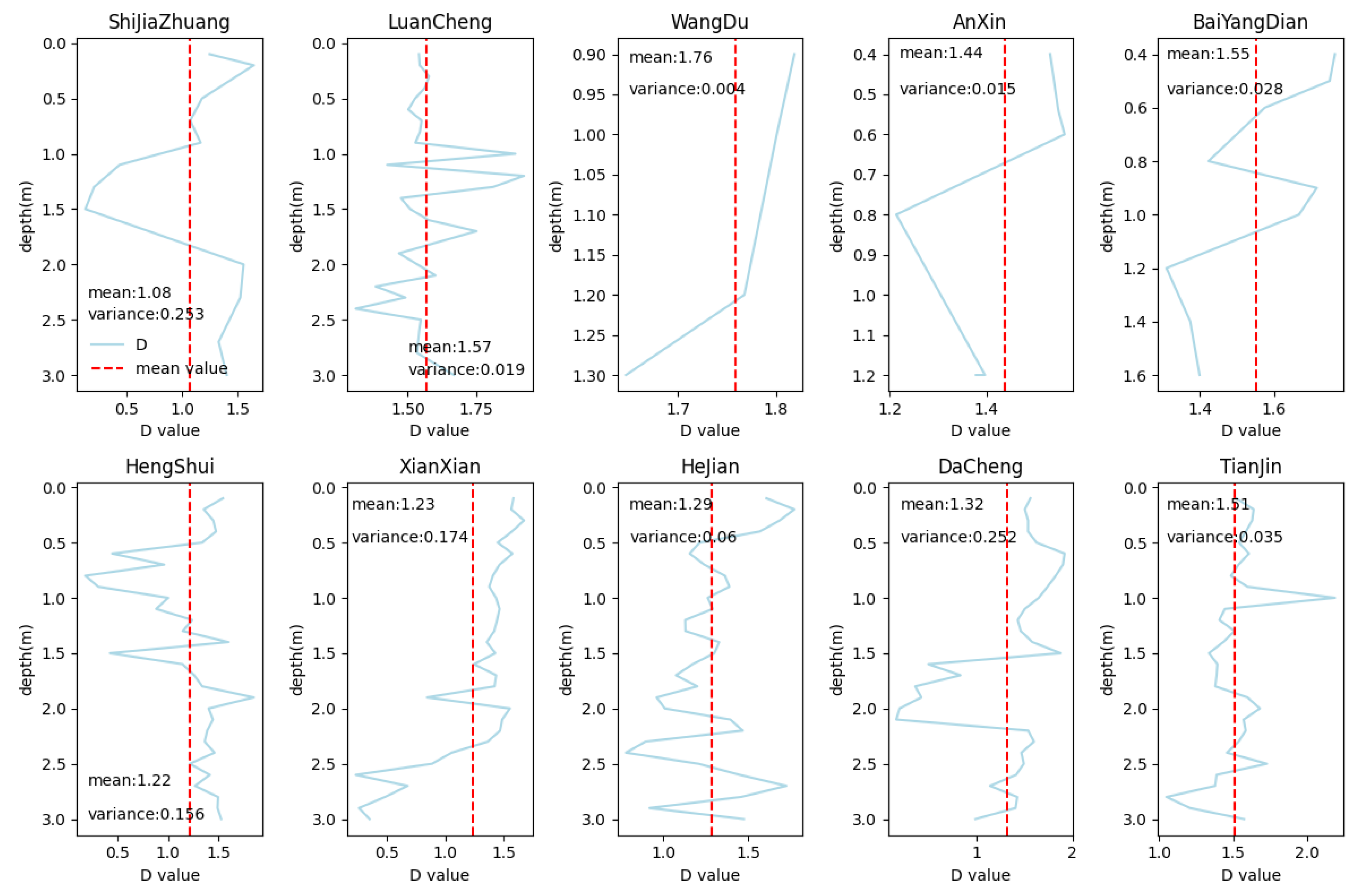
3.1. Soil Structure Profile Fractal Dimension (D-Value) Calculation

Based on Equation (1), the fractal dimensions (D values) of the soil structure were calculated for 207 samples from ten profiles spanning the piedmont, central plain, and coastal areas. After obtaining the D values for each profile at different depths, the mean and variance of the D values for each profile were calculated (Figure 2). The results show that the profile with the lowest mean D value was the Shijiazhuang profile in the piedmont area (1.08). The same profile also had the largest variance in D values, indicating a greater difference in soil particle sizes and greater variation in D values with depth compared to the central plain and coastal areas. In contrast, another piedmont profile, Luancheng, has a relatively large mean D value of 1.57 and a small variance of 0.019. This was attributed to the significant impact of long-term agricultural activities on the soil in the Luancheng profile. Both the Baiyangdian and Tianjin profiles show large mean D values that exceed 1.5 with small variances. This indicates that soil particle size differences decrease and tend towards finer particles as they move closer to coastal areas, with smaller variations in D values with depth. The Wangdu profile exhibited a large mean D value but a small variance, which can be attributed to the limited number of samples in this profile.

The spatial variation analysis of the soil D values at 12 depths across the ten profiles in the two river basins (Figure 3) showed that the maximum D value was 1.9017, occurring at a depth of 0.7 m. The minimum D value was 0.13, occurring at a depth of 1.5 m. At a depth of 0.2 m, the D value exhibited the smallest difference, only 0.414. At a depth of 1.5 m, the D value exhibited the largest difference, reaching 1.7468. The D value differences were relatively small for depths of 0.1–0.7 m, all less than one. Below a depth of 0.9 m, except for the depth of 2.3 m, the D value differences were all greater than one. Additionally, the three-dimensional spatial distribution of soil D values in the two river basins (Figure 4) indicated that at depths of 0.1–0.5 m, the D values were all greater than one. This depth corresponded to the cultivated layer, where the soil structure was relatively uniform. The spatial variation of D values was the greatest at depths of 0.9–2.0 m, where soil structure is most complex. Below a depth of 2.0 m, the spatial variation in the D values was smaller.

Clearly, the qualitative analysis above is insufficient to reveal patterns of soil structure variation in the two river basins and cannot quantify the spatial variability of D values on a large scale from the piedmont to the central plain to coastal areas. Further characterization using spatial analysis techniques is required to provide a more detailed understanding.

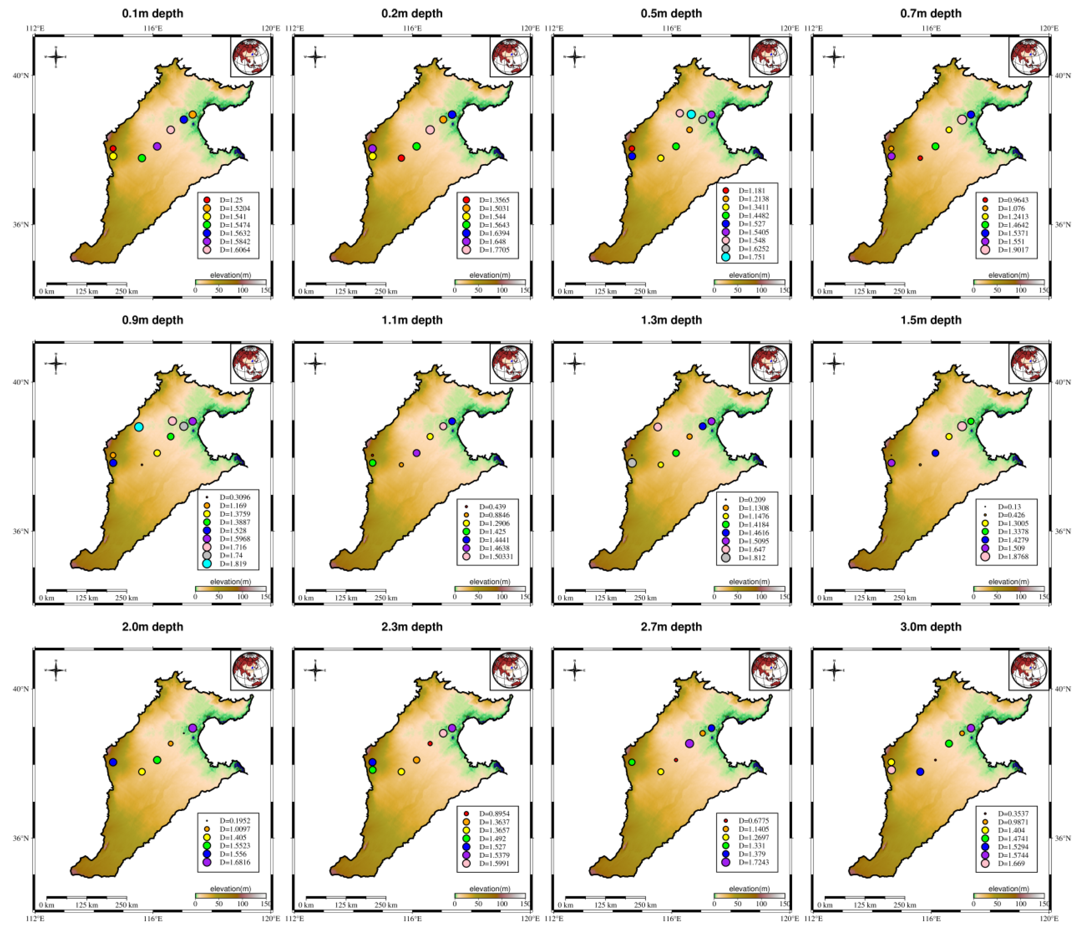
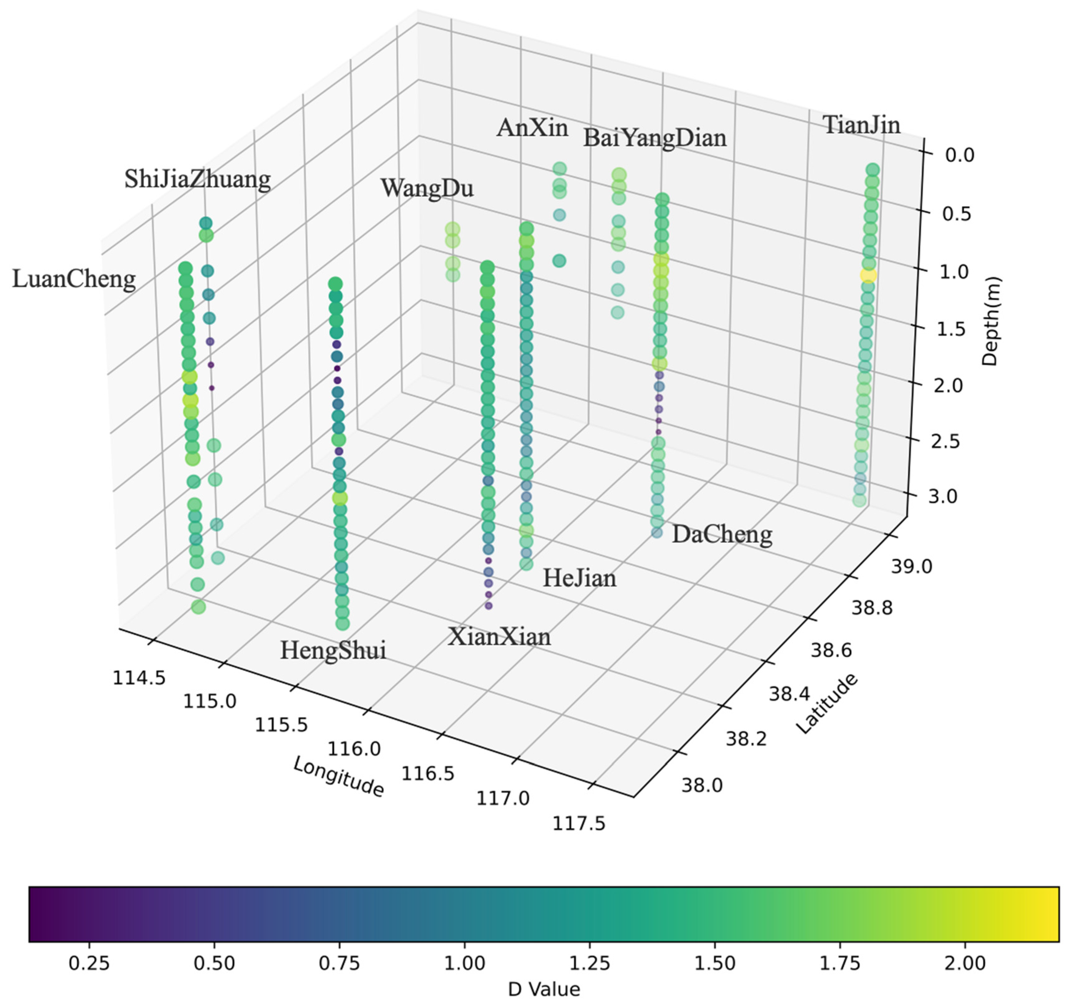
3.2. Spatial Variation of Soil Structure Fractal (D-Value) at the Basin Scale

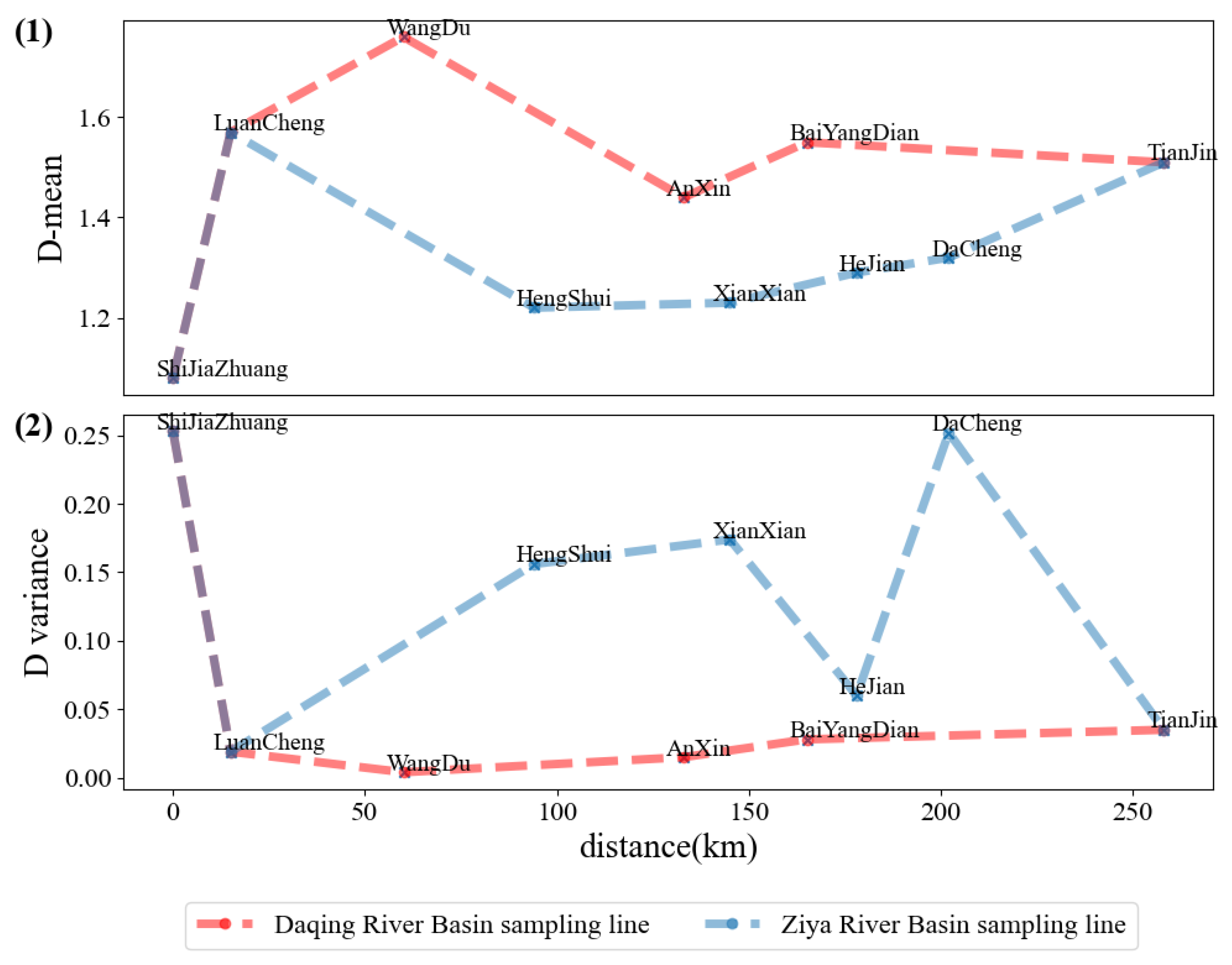
3.2.1. Spatial Variation of D Values in Two River Basins

Based on the “triangle” sampling line from Figure 1, the horizontal distances in the two river basins was determined, and the spatial variation of the mean D values and variance of mean D values were plotted, as shown in Figure 5(1),(2). In Figure 1, the horizontal distances from the Shijiazhuang profile to the other profiles in the Daqing River Basin from west to east are Luancheng (15 km), Wangdu (60 km), Anxin (133 km), Baiyangdian (165 km), and Tianjin (258 km), corresponding to the Daqing River Basin sampling line (red dashed line in Figure 5). Similarly, the horizontal distances from the Shijiazhuang profile to the other profiles in the Ziya River Basin from west to east are Luancheng (15 km), Hengshui (94 km), Xianxian (145 km), Hejian (178 km), Dacheng (202 km), and Binhai New Area (258 km), which correspond to the Ziya River basin sampling line (blue dashed line in Figure 5).

Overall, the mean soil D value in the Daqing River Basin was higher than that in the Ziya River Basin, and the variance was smaller than that in the Ziya River Basin (Figure 5). The mean soil D curves of the two river basins tended to be flat from the piedmont to the coastal area, as shown in Figure 5(1). The mean D value for the Daqing River basin was 1.4850, whereas the mean D value for the Ziya River basin was only 1.3171. Based on the fractal dimension calculation principle in Equation (1), the soil structure in the Ziya River Basin is more complex, and the distribution of soil particle size is more uneven than that in the Daqing River Basin. From the variance plot shown in Figure 5(2), the mean variance of soil D values in the Daqing River Basin was 0.059, whereas the mean variance of soil D values in the Ziya River Basin was as high as 0.136. This also confirms that the soil structure in the Ziya River Basin varies significantly among profiles, indicating greater spatial variability in soil structure fractals from the piedmont to the coast than in the Daqing River Basin.

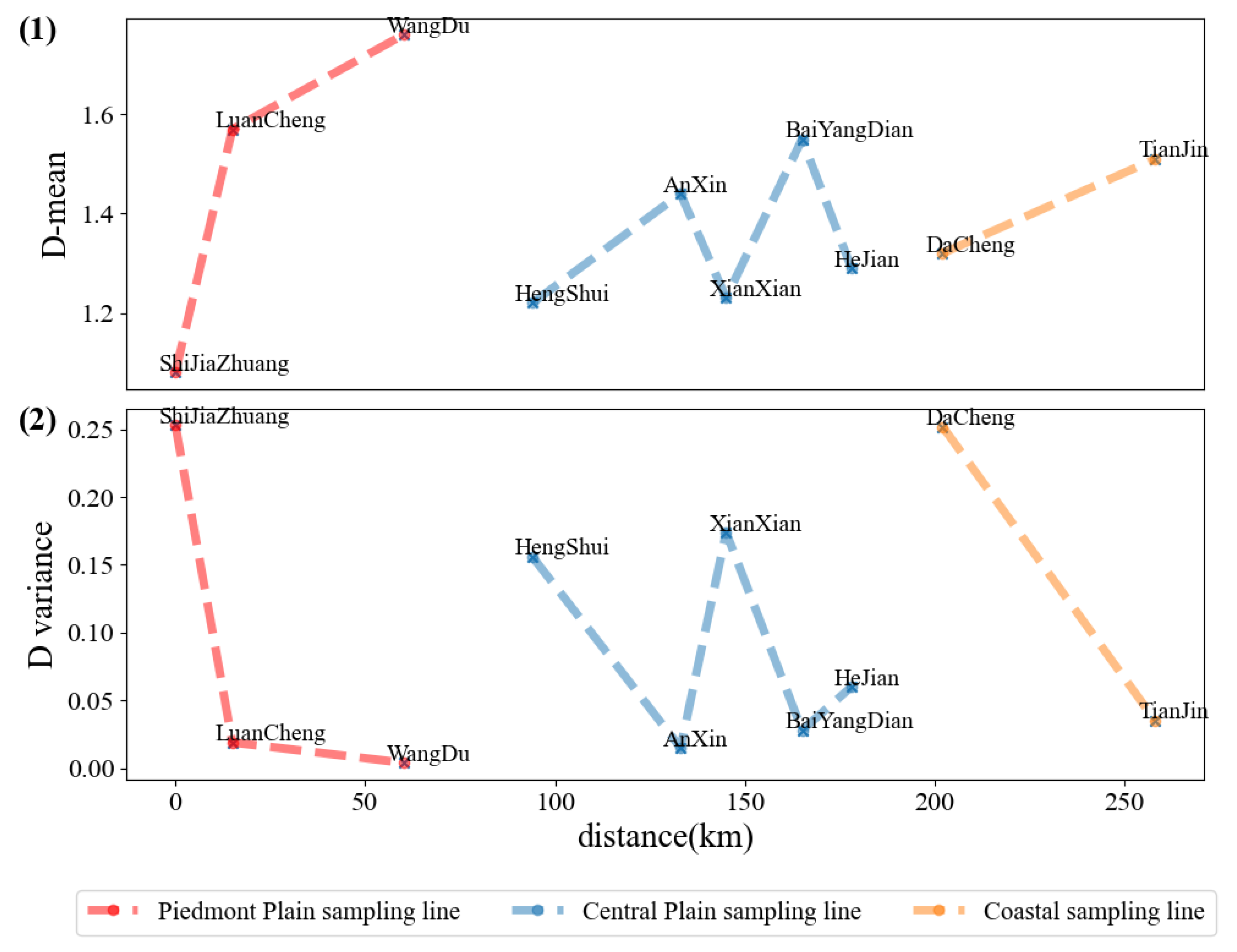
3.2.2. Spatial Variation of D Values in Piedmont Plain–Central Plain–Coastal Area

The piedmont, central plain, and coastal areas of the two river basins were analyzed together. Based on Figure 1, the spatial variation in mean D values and variance in D values from the piedmont plain to the central plain to the coastal areas on a basin scale were plotted, as shown in Figure 6(1),(2). Based on the sampling profile locations shown in Figure 1, the longitudinal distances from the Shijiazhuang and Luancheng profiles to the Wangdu profile are 67 km and 88 km, respectively. This formed the Daqing River Basin piedmont sampling line and piedmont–plain sampling line (red dashed line in Figure 6). From north to south, the longitudinal distances from the Baiyangdian, Hejian, Xianxian, and Hengshui profiles to the Anxin profile were 15, 51, 80, and 115 km, respectively. This formed the central plain sampling line (dashed blue line in Figure 6). The longitudinal distance from the Dacheng profile to the Tianjin profile was 32 km, forming a coastal area sampling line (yellow dashed line in Figure 6).

Overall, at the basin scale, the mean D values and variances were negatively correlated; that is, profiles with higher variance had lower mean values, and profiles with lower variance had higher mean values (Figure 6). The maximum and minimum mean D values were found in the piedmont profiles, as were the maximum and minimum variances in D values. The range of mean D values in coastal profiles was the smallest (1.32–1.51), indicating that from the piedmont to the coast, soil structure fractal becomes more uniform.

3.3. Spatial Variation Analysis

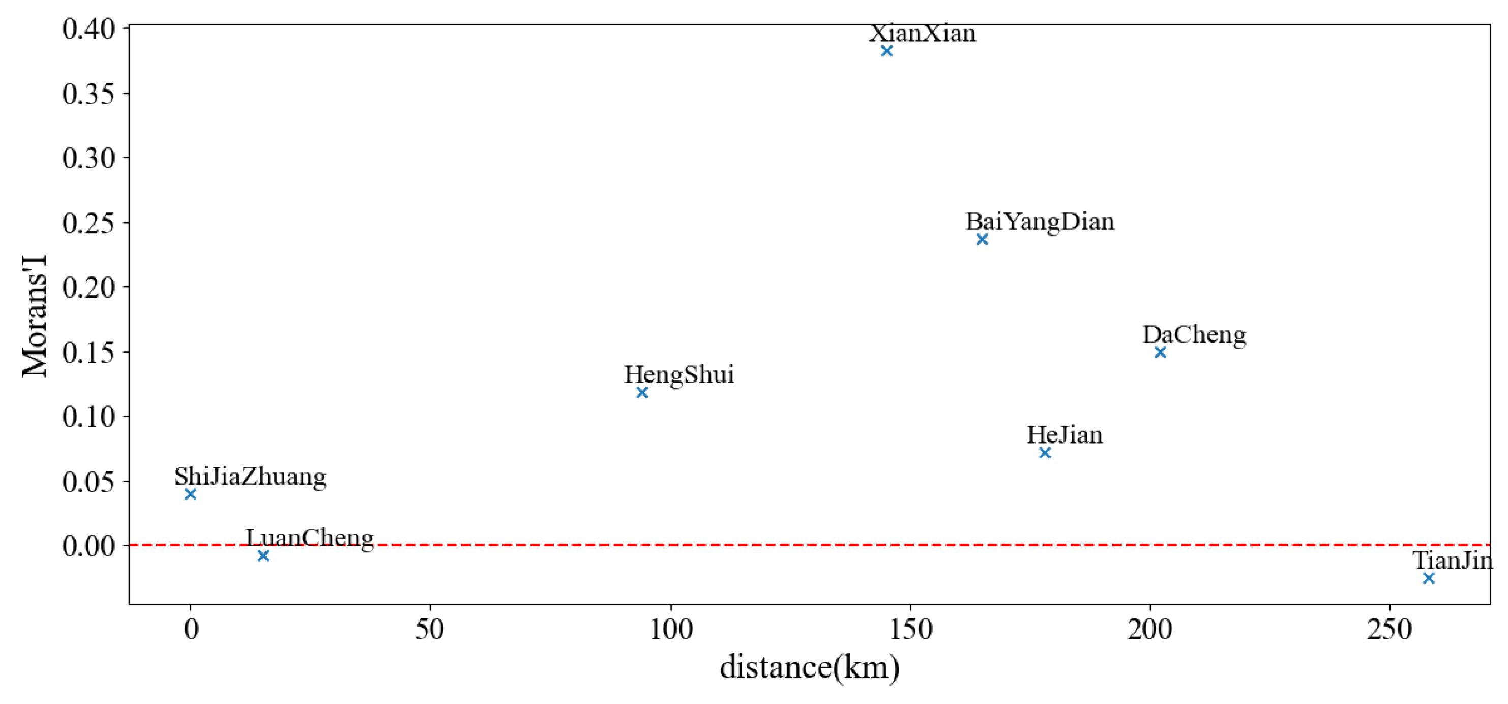
3.3.1. Spatial Autocorrelation Analysis of Profiles

A spatial autocorrelation analysis of each profile in the basin was performed. This study applied the global Moran’s I index to analyze the spatial autocorrelation of the soil D values for each profile (Figure 7). The weight matrix for the Moran’s I index calculation used the nearest neighbor matrix, which automatically calculated the threshold for neighbors based on the average sampling distance of each profile. According to the principles of detecting spatial autocorrelation using the Moran’s I index, the Moran’s I index for the Xianxian profile was 0.38, which is closest to one, indicating the highest degree of spatial autocorrelation. The Moran’s I indices for the Shijiazhuang, Luancheng, and Tianjin profiles were all below 0.05, approaching zero, indicating no significant spatial autocorrelation.

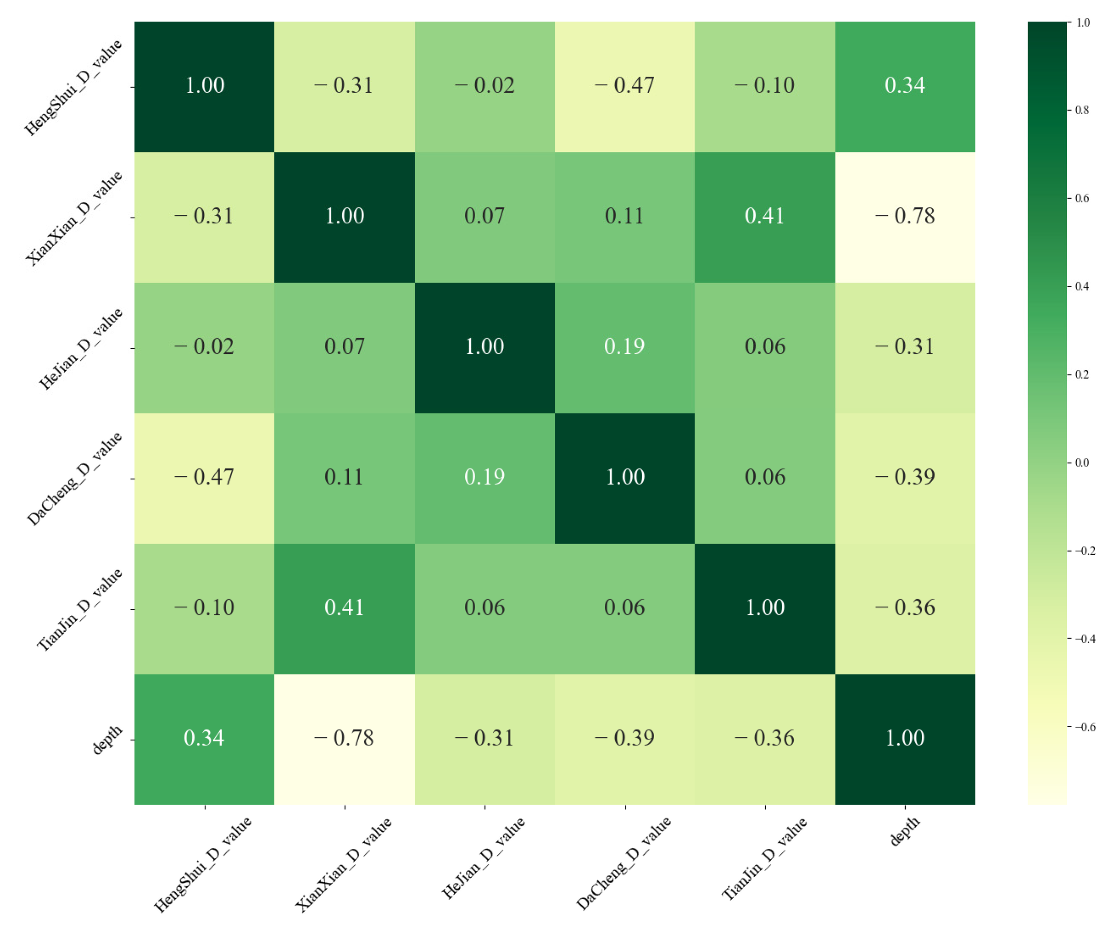
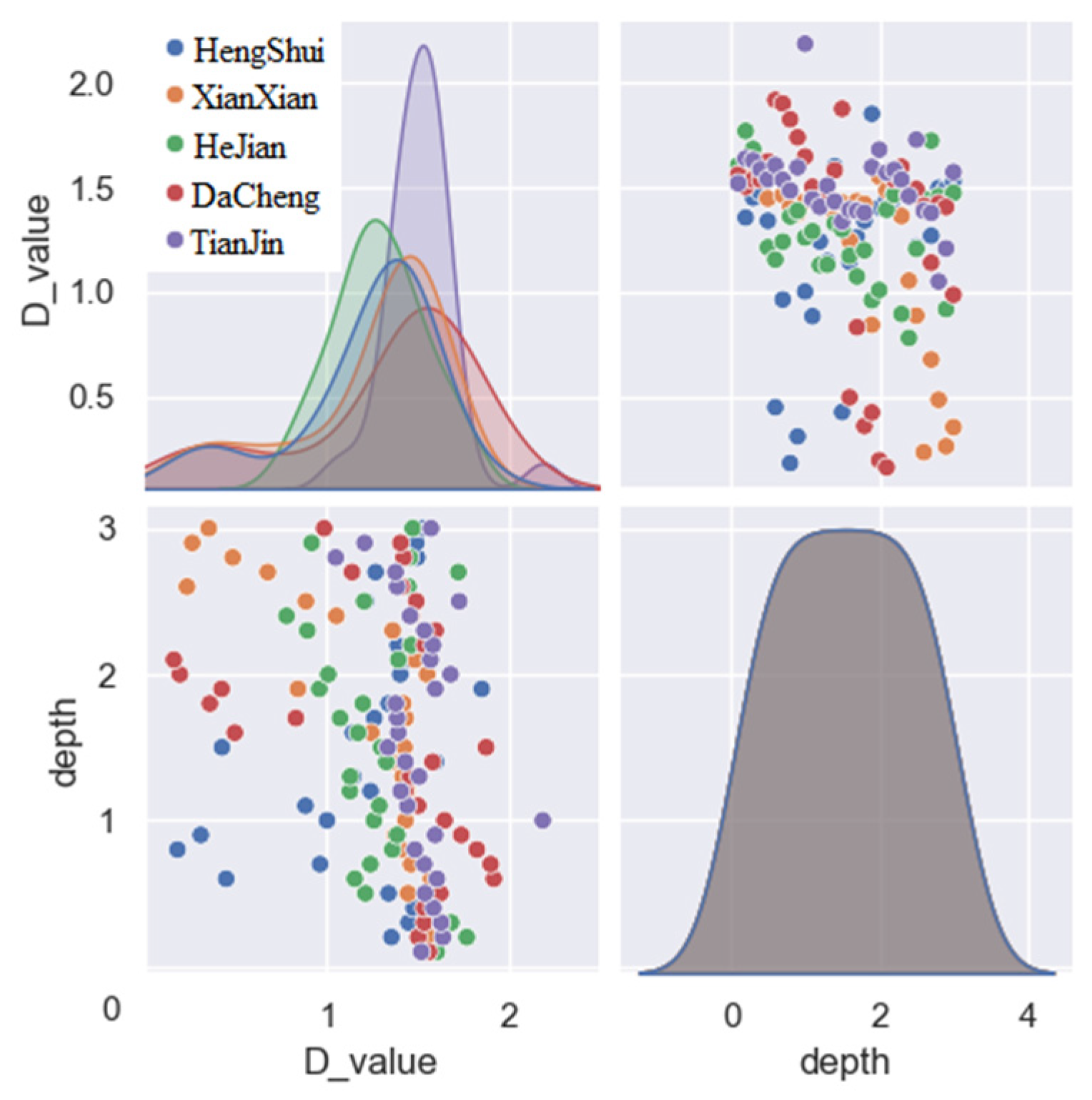
3.3.2. Spatial Correlation Analysis among Profiles

Profiles with the strongest spatial autocorrelation, that is, those with the highest global Moran’s I index, including Xianxian, Hengshui, Hejian, and Dacheng, and the profile with the weakest spatial autocorrelation, Tianjin, were subjected to an inter-profile correlation analysis. Depth was used as a factor in the correlation analysis to generate a correlation heatmap between D values and depth across the profiles (Figure 8). The data show that among the five profiles, the spatial correlation of D values is strongest between Hengshui and Dacheng (−0.47), whereas the spatial correlation of D values between other profiles is relatively low. The spatial correlation between Hengshui and Tianjin is only −0.095, indicating a strong spatial heterogeneity among these five profiles. Only the Xianxian profile exhibits a strong correlation between D values and depth (−0.78), indicating a strong spatial autocorrelation. As shown in the scatter plot matrix of the D values and depths for these five profiles (Figure 9), the D values for Hengshui and Dacheng did not follow a normal distribution (p < 0.05), whereas the D values for Xianxian, Hejian, and Tianjin did (p > 0.05). The distribution of the D values was relatively dispersed in the Dacheng and Hengshui profiles, whereas it was more concentrated in the Tianjin profile. The results for the Xianxian and Tianjin profiles strongly supported the conclusions of the global Moran’s I index analysis in Section 3.3.1.

3.3.3. Spatial Analysis Models

In this study, spatial analysis models, namely the semivariance function model, were established.

For the ten profiles in the two basins, the mean soil D values at four different layers (0–1, 1–2, 2–3, and 0–3 m) were calculated, and the K-S one-sample test was performed. Therefore, the numbers of samples for the four layers were ten, ten, seven, and ten. Because the p-values were all greater than 0.05 (

Table 2. K-S test and descriptive statistics of D value.

Soil Depth	Number of Samples	Mean	Median	Max	Min	Standard Deviation	CV(%)	Variance	Skewness	Kurtosis	K-S Test	p Value
0–1 m	10	1.502	1.543	1.81	1.008	0.219	14.569	0.048	−0.894	0.206	0.162	0.918
1–2 m	10	1.288	1.361	1.708	0.584	0.304	23.595	0.092	−0.913	0.469	0.194	0.78
2–3 m	7	1.308	1.409	1.51	0.827	0.213	16.284	0.045	−1.444	0.867	0.274	0.577
0–3 m	10	1.397	1.379	1.759	1.077	0.195	13.971	0.038	0.181	−0.838	0.153	0.947

), the null hypothesis could not be rejected, indicating that the samples followed a normal distribution and met the conditions for variogram analysis. In general, a coefficient of variation (CV) less than or equal to 0.1 indicates weak variability, 0.1–1 indicates moderate variability, and greater than 1 indicates strong variability, respectively. In this study, soil CVs at different depths were all between 0.1 and 1, indicating moderate variability. The CV of the 1–2 m soil layer was 23.595%, which was significantly higher than those of the 0–1 (14.569%) and 2–3 m (16.284%) layers. This quantified result is consistent with the qualitative analysis of the variation pattern of soil D values with depth, as described in Section 3.1.

Similarly, for the ten profiles within the two basins at depths of 0–1, 1–2, 2–3, and 0–3 m, the spatial distribution, variation, and correlation characteristics of soil D values were analyzed and described using anisotropic semivariograms in geostatistics. GS+ 9.0 was used for modeling, including linear, spherical, exponential, and Gaussian models. The criteria for selecting the fitting model were the highest R² and lowest RSS values. After comparing the four models, we found that the Gaussian model was suitable for the 0–1 and 1–2 m soil layers, whereas the exponential model was suitable for the 2–3 and 0–3 m soil layers (

Table 3. Anisotropic semivariance function model and parameters of fractal dimension D value of soil at different depths (GS+ 9.0 software).

Soil Depth	Fitting Model	Nugget C0	Sill C0 + C	Nugget to Sill (C0/(C0 + C))	Minimum Range (km−1)	Determination Coefficient (R2)	Residual Sum of Squares (RSS)
0–1 m	Gaussian model	0.03	0.246	0.122	152.4	0.21	0.0438
1–2 m	Gaussian model	0.072	0.6138	0.117	588.9	0.27	0.297
2–3 m	Exponential model	0.001	0.14	0.007	21.5	0.481	0.0156
0–3 m	Exponential model	0.024	0.16845	0.142	481.1	0.159	0.0284

). Kriging interpolation, spatial modeling, and random field interpolation were performed to visualize the spatial variation (Figure 10). Although the sample size was relatively small (37 samples), resulting in smaller R² values for each layer, all layers except the 2–3 m layer met the model analysis requirements, with the minimum range (21.5 km) being smaller than the sampling interval.

The spatial variability of each layer was determined based on the identified semivariogram models. The ratio of nugget to sill (C₀/(C₀ + C)) < 0.25 indicates a strong spatial correlation. In this study, the nugget-to-sill ratios for the 0–1, 1–2, and 0–3 m soil layers were all less than 0.25, indicating a strong spatial correlation in these layers.

4. Discussion

Through qualitative and quantitative analyses, on a basin scale, soil structure fractals were found to exhibit varying degrees of spatial variability, both in the plane and profile. Factors contributing to this large-scale spatial variability in soil structure fractals include both internal and external factors.

Internal factors stem from the inherent structural characteristics of soil, such as self-similarity and heterogeneity [23]. The application of fractal theory aims to use internal self-similarity to gain insight into the intricate structures hidden within chaotic phenomena [17]. Changes in these intricate structures cause spatial variability in the soil D values at different depths within the same profile, even with minimal depth variations [18]. The fundamental reasons for the spatial variability of soil D values include not only processing soil PSD data using fractal theory but also considering the physical significance of soil D values and their relationship to soil particle composition. External factors are the main reasons for the spatiotemporal evolution of the soil particle composition in the basin. These factors include the effects of climate change, geographical factors, and human activity on soil.

(1)

Physical Significance of Soil D Value and Its Role in Large-Scale Spatial Variation

The soil D value is an analysis of the spatial autocorrelation of different particle sizes at a certain depth of the soil profile [24]. It is an objective representation of the spatial distribution of soil particles at this depth and an analysis of small-scale spatial variability. This serves as a fundamental unit for spatial variability analyses at the basin scale. Therefore, the spatial variability analysis of the soil structure in this study included three levels: soil D values at a single depth, soil D values in a single profile, and basin soil D values across multiple profiles. Clearly, the results of the first-level spatial variability analysis have a crucial impact on those of the large-scale spatial variability analysis.

(2)

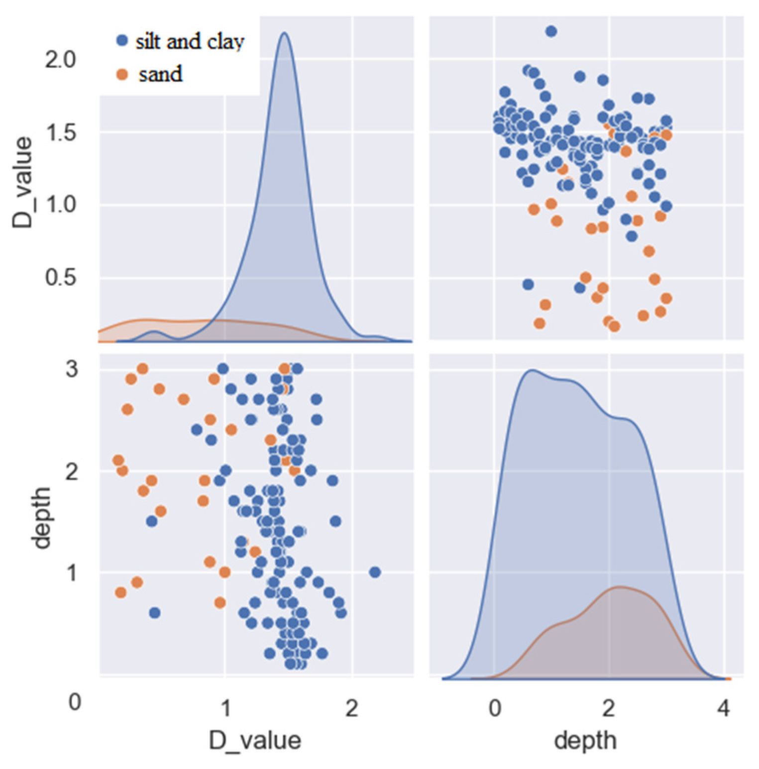
Relationship between Soil D Value and Soil Particle Composition

Differences in soil particle composition also determine the spatial variation in soil D values within the soil [18]. Following the selection of profiles in Section 3.3.2, the relationship between the soil D value and soil particle composition was analyzed for the Hengshui, Xianxian, Hejian, Dacheng, and Tianjin profiles. The particle compositions of 150 samples from different depths in the five profiles were analyzed according to the USDA textural classification (soil texture classification by the U.S. Department of Agriculture). The soil samples were named based on the percentage content of sand, silt, and clay, and classified into two categories: sandy soil (yellow dots) and silty clay (blue dots). These were then correlated with soil D values and depths, resulting in a scatter plot matrix of soil D values and depths for different soil types (Figure 11). The figure shows that sandy soils are found below a depth of 0.8 m, whereas silty clays are almost uniformly distributed at depths of 0 to 3 m. Soil D values for sandy soils are mainly concentrated between 0 and 1, whereas soil D values for silty clays follow a normal distribution, with most D values ranging between 1 and 2, peaking at approximately 1.5.

(3)

Relationship between Soil D Value Spatial Variation and Climate, Regional Changes, and Human-Intensive Activity

Climate change is a significant factor in the structural changes in basin soils. Since the Middle Pleistocene, the stratigraphy of the North China Plain has been characterized by fluvial environmental deposition [25]. Enhanced hydrodynamic conditions and a cold and arid climate, particularly during the Holocene, strengthened hydrodynamic conditions, resulting in a floodplain-dominated depositional environment. This period saw an increase in water levels in the lacustrine environment with the highest magnetic susceptibility values, which were positively correlated with medium silt. Moreover, intensive human activity irreversibly altered the soil structure. Uncontrolled groundwater extraction causes changes in the groundwater depth, resulting in changes in soil salinity [26]. Different land management practices affect soil bulk density and total porosity [27], thereby affecting soil structural changes and causing changes in saturated soil hydraulic conductivity.

In piedmont alluvial and floodplain areas, strong hydrodynamic action leads to coarse sediment particles, mainly sandy soil and silty sand, with sporadically distributed fine particles forming low-permeability lenses with limited distribution. In the central plain, fluvial and lacustrine deposits dominate, with a finer lithology in the vadose zone than in the piedmont plain, and the lenses gradually transition to interlayers. The eastern coastal plain is characterized by fine-grained sediments with clay and silty clay interlayers, and occasional sandy layers [28].

5. Conclusions

Using the PSD measurements of 207 soil samples from ten profiles in the Daqing River and Ziya River basins of the North China Plain, the quantifiable soil structure–soil structural fractal dimension (D) was obtained through single fractal theory. A large-scale spatial variation study of soil structural fractals at different depths across the piedmont plain coastal regions was conducted by combining various spatial analysis techniques, including the Moran’s I index, correlation heatmap analysis, K-S single-sample test, and geostatistical semivariogram functions.

• The mean, variance, and three-dimensional spatial distribution of soil D-values at the basin scale consistently showed that soil D-values tended to become more uniform from the piedmont to the coastal area. The closer one is to the coastal area, the smaller the differences in particle size, tending towards finer particles with less variation in depth. The maximum and minimum mean D-values were found in the piedmont profiles, and the variance in the D-values also exhibited their maximum and minimum values in the piedmont profiles. Coastal profiles show the smallest range of mean D-values (1.32–1.51). The mean variance of soil D-values in the Ziya River Basin was as high as 0.136, whereas it was 0.059 in the Daqing River Basin, indicating that the spatial variability of soil structural fractals in the Ziya River Basin was significantly larger than that in the Daqing River Basin.
• The results of the profile correlation analysis using the Moran’s I index method and heatmap analysis were consistent, showing that the Xian County profile had the highest degree of autocorrelation (Moran’s I index of 0.38) and the strongest correlation between the D-value and burial depth (−0.78). Inter-profile correlation analysis indicates that the Hengshui and Dacheng profiles have the strongest spatial correlation of soil D-values (−0.47), whereas the D-value correlations between other profiles are relatively low.
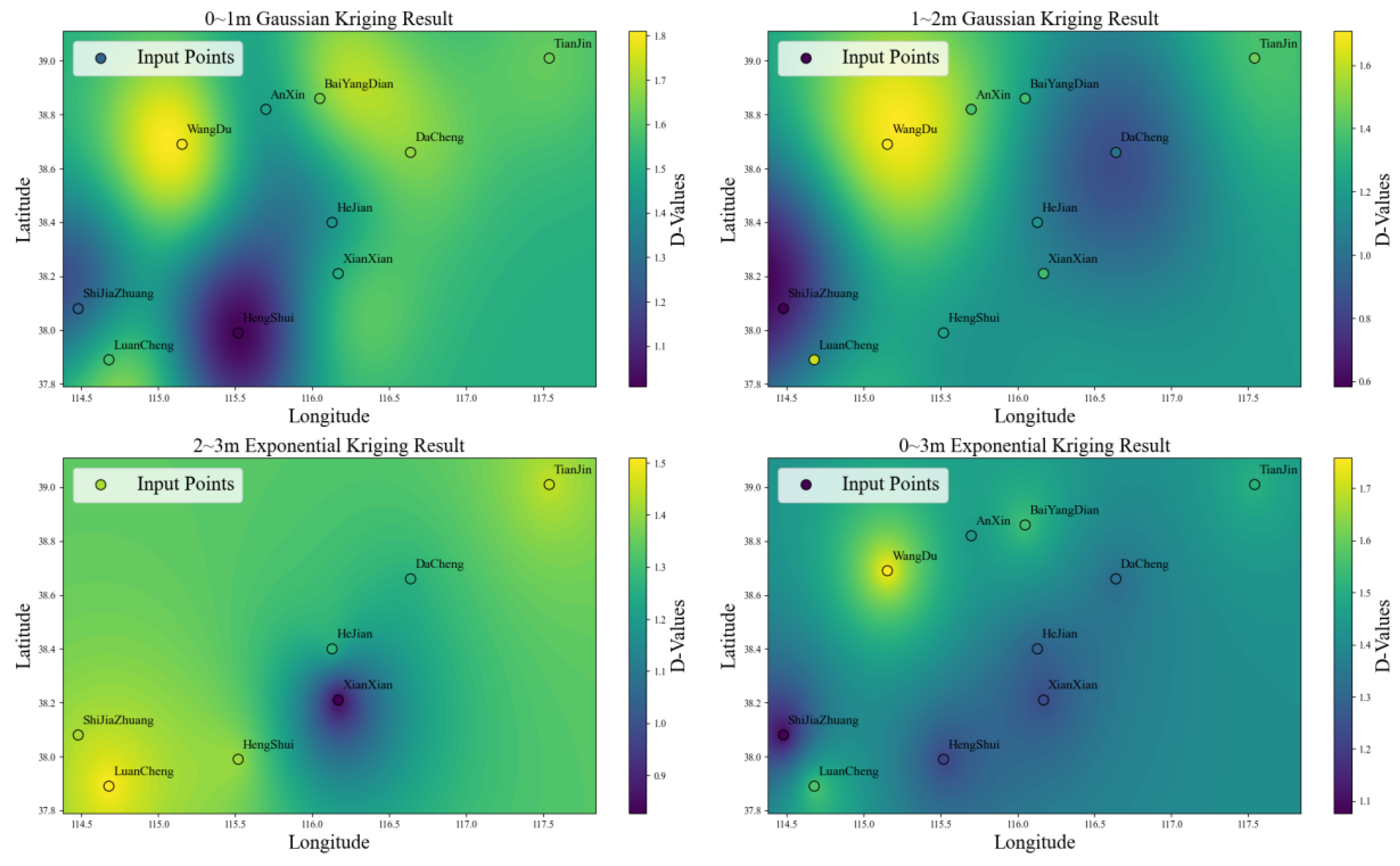
• Qualitative analysis, together with quantitative analysis results from the variogram and semivariance function models, consistently indicated that soil D-values exhibited the strongest spatial variability in the 1–2 m layer across all profiles in both basins. The coefficient of variation for the 1–2 m layer was 23.595%, which was significantly higher than those for the 0–1 m (14.569%) and 2–3 m (16.284%) layers. A Gaussian model was selected for the 0–1 and 1–2 m soil layers, whereas an exponential model was selected for the 2–3 and 0–3 m soil layers. In this study, the nugget-to-sill ratios for the 0–1, 1–2, and 0–3 m soil layers were all less than 0.25, indicating a strong spatial correlation across all layers.
• At the basin scale, soil structural fractals exhibited varying degrees of spatial variability in both the horizontal and vertical profiles. This variability results from the combined effects of internal and external factors, including the physical significance of soil D values, the relationship between soil D values and soil particle composition, climate change, geographic factors, and human activity. The specific contributions and mechanisms of these factors to the spatial variability of the soil structural fractals at different scales, ranges, and depths require further investigation.

In summary, our findings not only contribute to a deeper understanding of the fractal spatial variation of soil structure, but also provide practical applications for land management and environment planning. For instance, the insights gained from this study can inform policymakers and urban planners about the potential risks associated with soil erosion, landslides, and changes in soil fertility due to variations in soil structure fractals. By implementing appropriate measures such as improving soil conservation practices, establishing early warning systems for landslides, and developing sustainable agricultural practices, communities in the region can enhance their resilience and better protect human settlements against future challenges.

References

1. Han, Q.; Bai, H.; Liu, L.; Zhao, Y.; Zhao, Y. Model Representation and Quantitative Analysis of Pore Three-Dimensional Morphological Structure Based on Soil Computed Tomography Images. Eur. J. Soil Sci. 2020, 72, 1530–1542. [Google Scholar] [CrossRef]
2. Mohammadi, M.; Shabanpour, M.; Mohammadi, M.H.; Davatgar, N. Characterizing Spatial Variability of Soil Textural Fractions and Fractal Parameters Derived from Particle Size Distributions. Pedosphere 2019, 29, 224–234. [Google Scholar] [CrossRef]
3. Xie, J.; Liu, X.; Jasechko, S.; Berghuijs, W.R.; Wang, K.; Liu, C.; Reichstein, M.; Jung, M.; Koirala, S. Majority of Global River Flow Sustained by Groundwater. Nat. Geosci. 2024, 17, 770–777. [Google Scholar] [CrossRef]
4. Yang, H.-F.; Meng, R.-F.; Bao, X.-L.; Cao, W.-G.; Li, Z.-Y.; Xu, B.-Y. Assessment of Water Level Threshold for Groundwater Restoration and Over-Exploitation Remediation the Beijing-Tianjin- Hebei Plain. J. Groundwater Sci. Eng. 2022, 10, 113–127. [Google Scholar] [CrossRef]
5. Wang, Y.; Cao, F.; Li, R.M.; Ma, Z.S.; Guo, H.Q.; Ma, H. Geologic and Geochemical Evolutive Feature of Topsoil in Northland of Haihe River Piedmont Plain to Coastal Plain, China. Geol. Bull. China 2010, 29, 1210–1214. [Google Scholar]
6. Yuan, Y.; Zhang, T.L.; Zhang, C.; Ma, R. Spatial Variability of Vertical Permeability Coefficient from the Piedmont to the Coastal Area of Notrh China Plain. South-North Water Divers. Water Sci. Technol. 2020, 18, 184–190. [Google Scholar] [CrossRef]
7. He, Y.P. Shallow Groundwater Hydrogeochemical Simulation Modeling from Piedmont Plain to Coastal Plain Shallow Area in the North Chian Plain. Master’s Thesis, China University of Geoscience, Beijing, China, 2012. [Google Scholar]
8. Lee Peyton, R.; Gantzer, C.J.; Anderson, S.R.; Haeffner, B.; Pfeifer, P. Fractal Dimension to Describe Soil Macropore Structure Using X Ray Computed Tomography. Water Resour. Res. 1994, 30, 691–700. [Google Scholar] [CrossRef]
9. Xia, Y.; Cai, J.; Wei, W.; Hu, X.; Wang, X.; Ge, X. A New Method for Calculating Fractal Dimensions of Porous Media Based on Pore Size Distribution. Fractals 2018, 26, 1850006. [Google Scholar] [CrossRef]
10. Kong, B.; He, S.-H.; Tao, Y.; Xia, J. Pore Structure and Fractal Characteristics of Frozen–Thawed Soft Soil. Fractal Fract. 2022, 6, 183. [Google Scholar] [CrossRef]
11. Yuan, B.; Li, Z.; Chen, W.; Zhao, J.; Lv, J.; Song, J.; Cao, X. Influence of Groundwater Depth on Pile–Soil Mechanical Properties and Fractal Characteristics under Cyclic Loading. Fractal Fract. 2022, 6, 198. [Google Scholar] [CrossRef]
12. Prosperini, N.; Perugini, D. Particle Size Distributions of Some Soils from the Umbria Region (Italy): Fractal Analysis and Numerical Modelling. Geoderma 2008, 145, 185–195. [Google Scholar] [CrossRef]
13. Armstrong, A.C. On the Fractal Dimensions of Some Transient Soil Properties. J. Soil Sci. 1986, 37, 641–652. [Google Scholar] [CrossRef]
14. Fu, X.; Ding, H.; Sheng, Q.; Zhang, Z.; Yin, D.; Chen, F. Fractal Analysis of Particle Distribution and Scale Effect in a Soil–Rock Mixture. Fractal Fract. 2022, 6, 120. [Google Scholar] [CrossRef]
15. Wang, Z.; Luo, Y.; Luo, W.; Deng, X. Mechanical Characterization and Parameter Identification of Rheological Deformation of Subgrade Compacted Soil. Chin. J. Rock Mech. Eng. 2011, 30, 208–216. [Google Scholar]
16. Sun, Y.; Gao, Y.; Ju, W. Fractional Plasticity and Its Application in Constitutive Model for Sands. Chin. J. Geotech. Eng. 2018, 40, 1535–1541. [Google Scholar] [CrossRef]
17. Anderson, A.N.; McBratney, A.B.; Crawford, J.W. Applications of Fractals to Soil Studies. Adv. Agron. 1997, 63, 1–76. [Google Scholar] [CrossRef]
18. He, Y.; Lv, D. Fractal Expression of Soil Particle-Size Distribution at the Basin Scale. Open Geosci. 2022, 14, 70–78. [Google Scholar] [CrossRef]
19. Westerholt, R. A Simulation Study to Explore Inference about Global Moran’s I with Random Spatial Indexes. Geogr. Anal. 2022, 55, 621–650. [Google Scholar] [CrossRef]
20. Lilliefors, H.W. On the Kolmogorov-Smirnov Test for Normality with Mean and Variance Unknown. J. Am. Stat. Assoc. 1967, 62, 399–402. [Google Scholar] [CrossRef]
21. Sun, X.; Guo, C.; Zhang, J.; Sun, J.; Cui, J.; Liu, M. Spatial-Temporal Difference between Nitrate in Groundwater and Nitrogen in Soil Based on Geostatistical Analysis. J. Groundwater Sci. Eng. 2023, 11, 37–46. [Google Scholar] [CrossRef]
22. Ersahin, S. Comparing Ordinary Kriging and Cokriging to Estimate Infiltration Rate. Soil Sci. Soc. Am. J. 2003, 67, 1848–1855. [Google Scholar] [CrossRef]
23. Ersahin, S.; Gunal, H.; Kutlu, T.; Yetgin, B.; Coban, S. Estimating Specific Surface Area and Cation Exchange Capacity in Soils Using Fractal Dimension of Particle-Size Distribution. Geoderma 2006, 136, 588–597. [Google Scholar] [CrossRef]
24. He, Y.; Wang, G. Identifying the Soil Structure of the Piedmont–Plains by the Fractal Dimension of Particle Size. Soil Water Res. 2019, 14, 212–220. [Google Scholar] [CrossRef]
25. Wang, C.; Song, J.; Tan, L.; Lv, M. Characteristics of Grain Size and Magnetic Susceptibility of Sediments and Their Environmental Significance in Piedmont Plain of Mt. Taihang since Early Pleistocene. J. Hebei Geo. Univ. 2023, 46, 14–20. [Google Scholar] [CrossRef]
26. Xiong, Y.; Xi, C.F.; Zhang, T.L. Studies on the Soils of the Yellow River Valley II. Genesis and Evolution of the Soils of North China Greate Plain. Acta Pedol. Sin. 1958, 6, 25–43. [Google Scholar]
27. Chang, X.L. Characteristics and Influencing Factors of Soil Saturated Water Conductivity under Different Land Use Modes in North China Plain. Water Sav. Irrig. 2023, 7, 28–33. [Google Scholar] [CrossRef]
28. Huo, S.Y. Research on the Effect of Water Table Decline on Vertical Groundwater Recharge: A Case Study in the North China Plain. Ph.D. Thesis, China University of Geoscience, Wuhan, China, 2015. [Google Scholar]
Figure 1. Location map of the study area (note: the Figure is referenced from the literature [18]).
Fractalfract 08 00570 g001
Figure 2. Variation of soil D values with depth for each profile. Blue solid line: trend of D values with depth; red dashed line: mean D value for the profile and variance of D values within the profile (variance).
Fractalfract 08 00570 g002
Figure 3. Spatial variation of soil D values at different depths. The color and radius of the circles together represent variation trends in D values at the same depth. Color indicates grade and radius indicates size.
Fractalfract 08 00570 g003
Figure 4. Three-dimensional spatial distribution of soil D values at the basin scale (note: The size of the circles represents the magnitude of the D-values, with larger circles indicating higher D-values and smaller circles indicating lower D-values).
Fractalfract 08 00570 g004
Figure 5. Spatial variation of mean soil D values (D-mean) and variance (D-variance) in two river basin profiles. Note: (1) trend of D-mean with distance; (2) trend of D-variance with distance.
Fractalfract 08 00570 g005
Figure 6. Spatial variation of mean soil D values (D-mean) and variance (D-variance) in piedmont–central plain–coastal area profiles. Note: (1) trend of D-mean with distance; (2) trend of D-variance with distance.
Fractalfract 08 00570 g006
Figure 7. Global Moran’s I indices for different profiles (note: The red dashed line indicates where the global Moran’s I index equals 0, signifying a random spatial distribution of the data, meaning no significant spatial autocorrelation. Values above the dashed line suggest a certain degree of positive spatial correlation, while values below the dashed line indicate some level of negative spatial correlation).
Fractalfract 08 00570 g007
Figure 8. Heat map of correlation analysis between D values and buried depth among basin profiles.
Fractalfract 08 00570 g008
Figure 9. Scatter matrix diagram of soil D values and depth of each profile at the basin scale (note: Different colors represent the soil profiles from various sampling sites).
Fractalfract 08 00570 g009
Figure 10. Kriging interpolation plots of soil D values at different depths of the basin scale.
Fractalfract 08 00570 g010
Figure 11. Scatter matrix of soil D value and the buried depth of different soil types at the basin scale (note: Different colors represent the soil profiles from various sampling sites).
Fractalfract 08 00570 g011