A Collocation Numerical Method for Highly Oscillatory Algebraic Singular Volterra Integral Equations

Abstract

The highly oscillatory algebraic singular Volterra integral equations cannot be solved directly. A collocation numerical method is proposed to overcome the difficulty created by the highly oscillatory algebraic singular kernel. This paper is composed primarily of two methods—the piecewise constant collocation method and the piecewise linear collocation method—in which uniformly distributed nodes serve as collocation points. For the efficient computation of highly oscillatory and algebraic singular integrals, the steepest descent method as well as the Gauss–Laguerre and generalized Gauss–Laguerre quadrature rules are employed. Consequently, the resulting linear system is solved for the unknown function approximated by the Lagrange interpolation polynomial. Detailed theoretical analysis is carried out and numerical experiments showing high accuracy are also presented to confirm our analysis.

1. Introduction

Integral equations play a crucial role in modeling and analyzing a wide range of scientific and engineering phenomena [1,2,3]. Mathematical physics models such as diffraction, quantum scattering, conformal mapping, and water waves have also led to the development of integral equations [4,5,6,7]. Electro–mechanical devices can be modeled effectively using integral models to analyze their dynamic behavior: for example, to simulate the angular velocity of a wind turbine [8] and to evaluate the current performance of a reluctance motor [9].

Various initial and boundary value problems can also be reformulated as Volterra or Fredholm integral equations. Volterra integral equations (VIEs) have been the focus of much research: both theoretical and numerical. VIEs can be applied to create mathematical models for a vast array of phenomena including epidemic diffusion, demography, insurance mathematics, reaction processes, electromagnetic scattering, viscoelastic materials, population dynamics, biological interactions, fish propagation, heat transfer, and heat radiation [10,11,12,13,14,15,16]. For instance, the Helmholtz equation

$$\Delta y+{\omega }^{2}y=0\mathrm{in}{R}^{\eta }\setminus \overline{\Omega },\eta =2,3$$

is a traditional model for describing the scattering of time-harmonic acoustic or electromagnetic wave problems. Under suitable boundary conditions, it can be expressed as an integral equation

$$y\left(x\right)={\int }_{\Gamma }y\left(t\right)\frac{\partial \xi (x,t)}{\partial n\left(t\right)}-\xi (x,t)\frac{\partial y}{\partial n\left(t\right)}ds\left(t\right),x\in R^{\eta }\setminus \overline{\Omega }$$

with

$$\xi (x,t)=\left\{\begin{array}{cc}\frac{i}{4}{H}_0^1\left(\omega \right|x-t\left|\right)\hfill & \eta =2\hfill \\ \frac{1}{4\Pi }\frac{e^{i\omega |x-t|}}{|x-y|}\hfill & \eta =3\hfill \end{array}\right.,$$

where the given kernel function $\xi (x,t)$ is weakly singular and highly oscillatory for $\omega \gg 1$ [17,18,19].

This paper analyzes the highly oscillatory algebraic singular VIEs of the second kind of the form

$$y\left(x\right)+{\int }_0^x\frac{K(x,t)e^{i\omega g(x,t)}}{{(x-t)}^{\alpha }{t}^{\beta }}y\left(t\right)dt=f\left(x\right),x\in [0,1],$$

(1)

where $\alpha ,\beta <1$, $K(x,t)$ is a continuous function, $f\left(x\right)$ is a given function, and y(x) is the unknown function that must be determined. For different cases, based on $K(x,y),\alpha ,\beta ,\omega$ the theoretical aspects of the solutions, their uniqueness, and the existence of VIEs with singularities have been thoroughly studied and established; see [20,21]. Attaining an analytical solution for a highly oscillatory algebraic singular VIE (1) proves to be a formidable challenge. Especially, when $K(x,t)\ne 0,\alpha ,\beta <1,$ and $\omega \gg 1$, the solution to (1) is both singular and highly oscillatory. In recent decades, computational methods for evaluating highly oscillatory integrals have undergone significant advancements. Among numerical methods for VIEs, spectral methods have gained more interest from researchers. Some of the eminent methods are the differential transform method [22,23,24], Filon-type method [25], Levin’s method [26], Galerkin and multi Galerkin methods [27], Chebyshev wavelet method [28], collocation method [29], Jacobi spectral collocation method [30,31], Chelyshkov collocation method [32,33], and the collocation boundary value method [34].

The weakly singular VIE of the second kind with highly oscillatory Bessel kernels of the type

$$y\left(x\right)+{\int }_0^x\frac{J_m\left(\omega (x-t)\right)}{{(x-t)}^{\alpha }}y\left(t\right)dt=f\left(x\right),x\in [0,1],0\le \alpha <1,$$

(2)

is discussed by Xiang and Brunner [35]. The authors explore the Filon method, piecewise constant collocation method (PCCM), and piecewise linear collocation method (PLCM) to get the approximated solution of (2). It was claimed that the solution of the VIE is uniformly bounded for $\omega \gg 1$ and the computational cost of the presented method remains the same regardless of the size of the frequencies. A direct Hermite collocation method as well as a piecewise Hermite collocation method are presented for VIEs of the second kind with highly oscillatory Bessel kernels by Fang et al., see [36]. The results of this study showed that Hermite-type collocation methods are more reliable than other collocation methods. The authors claimed that the approximate function value and derivative value can be calculated concurrently by both methods.

Fermo and Occorsio [37] presented the $Nystr\ddot{o}m$ method for algebraic singular VIEs:

$$y\left(x\right)+{\int }_{-1}^{x}K(x,t){(x-t)}^{\alpha }{(1+t)}^{\beta }y\left(t\right)dt=f\left(x\right),x\in (-1,1),\alpha ,\beta >-1,$$

(3)

where the kernel function possesses singularities along the diagonal $x=t$ and/or at $x=-1$. The authors provided the stability, convergence, and error analysis in the Zygmund weighted space. However, the kernel function presented there does not contain the oscillatory function, i.e., $\omega =0$. Li et al. [38] proposed the Chebyshev and Legendre pseudo-spectral method for weakly singular VIEs of the second kind (3) with $\beta =0$. The integral operator in the equation is approximated by the Gauss-type quadrature formula. They also proved the exponential convergence of the proposed method. A Chebyshev collocation method is developed by Wang et al. [39] to solve VIEs with algebraic or logarithmic singularities by splitting the interval into a singular subinterval and a regular subinterval. To approximate the solution directly in the singular subinterval, the truncated asymptotic expansion or its Padé approximation is used. The singular kernel is evaluated analytically by using a stable and fast recurrence algorithm.

Wu and Sun [40] presented a collocation method based on the steepest descent method for weakly singular VIEs with highly oscillatory kernels:

$$y\left(x\right)+{\int }_0^x\frac{K(x,t)e^{i\omega g(x,t)}}{{(x-t)}^{\alpha }}y\left(t\right)dt=f\left(x\right),x\in [0,1].$$

(4)

After applying the steepest descent method, the introduced method calculated the highly oscillatory integral with the generalized Gauss–Laguerre rule. Xiang and Wu [41] introduced piecewise constant and piecewise linear collocation methods for approximating the solution to VIEs of the second kind with weakly singular trigonometric kernels. The authors stated that a Filon-type method can be used to compute oscillatory integrals by evaluating the highly oscillatory kernels of integral equations. According to Liang and Brunner, the convergence order of the piecewise collocation method for weakly singular VIEs of the second kind has been improved: see [42] for more details. With an increase in n, a piecewise polynomial collocation method with degree $m=1$ is presented to improve the convergence order. For weakly singular VIEs of the second kind with oscillatory trigonometric kernels, Wu [43] compared the collocation method on uniform meshes with that on graded meshes by using the Filon-type method to compute the highly oscillatory integrals occurring in the collocation equation. The author demonstrated that as long as the kernels are oscillatory trigonometric, collocation on graded meshes may not be better than on uniform meshes. It is evident from the above discussion that the discussed methods are inapplicable for solving (1) directly due to the highly oscillatory and algebraic singular kernel. This paper aims to develop an efficient numerical method to compute VIEs with highly oscillatory and algebraic singular kernels. To calculate (1), we have proposed two collocation methods depending on the uniform mesh: the PCCM and the PLCM. Based on the analytic continuation, the steepest descent method is used to compute the obtained highly oscillatory algebraic singular integrals. This transforms them into the sum of two line integrals, with integrands that are nonoscillatory and decay exponentially fast. These line integrals can be efficiently computed by the Gauss–Laguerre and generalized Gauss–Laguerre quadrature rules. In addition, some theoretical and numerical results are also provided to prove the validity of the proposed method.

Here is the brief outline of the paper. Section 1 provides a brief introduction to numerical methods for the VIEs for different cases. The purpose of Section 2 is to present the basic conceptual information and methodology of the proposed method for approximating highly oscillatory algebraic singular VIEs. Section 3 provides some theoretical results, including error bounds for the introduced novel method. Section 4 promises to represent the accuracy and efficiency of the proposed method with some numerical examples. Moreover, a comparison is made between the new numerical technique and the one provided by Wu [43] to demonstrate its reliability.

2. Description of the Collocation Methods

This section explores numerical techniques for computing the solution to (1). A direct method for evaluating highly oscillatory algebraic singular VIEs is the PCCM. Suppose that

$$I_h=\{x_n=nh,0\le n\le N,h=\frac{T}{N}\}$$

(5)

as a uniform mesh of the interval $I=[0,T]$. Let ${\sigma }_n=(x_n,x_{n+1})$, and the set of collocation points is defined by

$$X_h=\{x=x_{n,j}=x_n+c_{j}h;0\le c_1<\dots <c_m\le 1,0\le n\le N-1\},$$

(6)

where $c_j$ is the collocation parameter that determines $X_h$. For a given mesh $I_h$, the piecewise polynomial space $S_{\rho }^{\left(d\right)}\left(I_h\right)$, with $\rho \ge 0,-1\le d\rho$, is given by

$$S_{\rho }^d\left(I_h\right)=\{v\in C^d\left(I\right){:v|}_{{\sigma }_n}\in {\pi }_{\rho },0\le n\le N-1\}.$$

Here, ${\pi }_{\rho }$ represents the space of polynomials with a degree of at most $\rho$. For VIEs, the particular piecewise polynomial space $S_{m+d}^d\left(I_h\right)$ with $\rho =m+d,m\ge 1,d\ge -1$; we choose $d=-1$. Then, the natural collocation space is $S_{m-1}^{(-1)}\left(I_h\right)$ with dimension $Nm$.

The PCCM considers the collocation points ${\tilde{x}}_n\in [x_n,x_{n+1}],n=0,1,\cdots ,N-1$; then, the approximate function $\tilde{y}\left(x\right)$ of $y\left(x\right)$ such that $\tilde{y}{\left(x\right)|}_{[x_n,x_n+1)}$ is constant. However, for the PLCM, $\tilde{y}{\left(x\right)|}_{[x_n,x_n+1]}$ is linear such that $\tilde{y}\left(x_n\right)=y\left(x_n\right)$ and $\tilde{y}\left(x_{n+1}\right)=y\left(x_{n+1}\right)$. The core purpose of the PCCM and PLCM is to find the approximate solution in $S_{m-1}^{(-1)}\left(I_h\right)$. Set $Y_{n,i}=y_h\left(x_{n,i}\right)$; the collocation polynomial $y_h\left(x\right)\in S_{m-1}^{(-1)}\left(I_h\right)$ on ${\sigma }_n$ is expressed as

$$y_h\left(x\right)=y_h(x_n+th)=\sum _{j=1}^m{L}_j\left(t\right)Y_{n,j},t\in (0,1],$$

(7)

where $L_j\left(t\right)={\prod }_{k\ne j}^m\frac{t-c_k}{c_j-c_k}$. Then, for $x=x_{n,j},g(x,t)=(x-t)$, Equation (1),

$$y_h\left(x\right)+{\int }_0^x\frac{K(x,t)e^{i\omega (x-t)}}{{(x-t)}^{\alpha }{t}^{\beta }}{y}_h\left(t\right)dt=f\left(x\right),x\in X_h,$$

can be rewritten as

$$\begin{array}{cc}\hfill y_h\left(x_{n,j}\right)=& f\left(x_{n,j}\right)-{\int }_0^{x_n+c_{j}h}\frac{K(x_{n,j},t)e^{i\omega (x_{n,j}-t)}}{{(x_{n,j-t}-t)}^{\alpha }{t}^{\beta }}{y}_h\left(t\right)dt,\hfill \\ \hfill =& f\left(x_{n,j}\right)-\sum _{l=0}^{n-1}{\int }_{x_l}^{x_{l+1}}\frac{K(x_{n,j},t)e^{iw(x_{n,j}-t)}}{{(x_{n,j}-t)}^{\alpha }{t}^{\beta }}{y}_h\left(t\right)dt-{\int }_{x_n}^{x_{n+c_{j}h}}\frac{K(x_{n,j},t)e^{iw(x_{n,j}-t)}}{{(x_{n,j}-t)}^{\alpha }{t}^{\beta }}{y}_h\left(t\right)dt,\hfill \\ \hfill =& f\left(x_{n,j}\right)-\sum _{l=0}^{n-1}h{\int }_0^1\frac{K(x_{n,j},x_l+th)e^{iw(x_{n,j}-x_l-th)}}{{(x_{n,j}-x_l-th)}^{\alpha }{(x_l+th)}^{\beta }}{y}_h(x_l+th)dt\hfill \\ \hfill & -h{\int }_0^{c_j}\frac{K(x_{n,j},x_n+th)e^{iw(x_{n,j}-x_n-th)}}{{(x_{n,j}-x_n-th)}^{\alpha }{(x_n+th)}^{\beta }}{y}_h(x_n+th)dt.\hfill \end{array}$$

Now by approximating $y_h\left(x_{n,j}\right)$ by the Lagrange polynomial (7), we get

$$\begin{array}{cc}\hfill Y_{n,j}=& f\left(x_{n,j}\right)-h\sum _{l=0}^{n-1}\sum _{k=1}^m{Y}_{l,k}{\int }_0^1\frac{K(x_{n,j},x_l+th)e^{iw(x_{n,j}-x_l-th)}}{{(x_{n,j}-x_l-th)}^{\alpha }{(x_l+th)}^{\beta }}{L}_k\left(t\right)dt\hfill \\ \hfill & -h\sum _{k=1}^m{Y}_{n,k}{\int }_0^{c_j}\frac{K(x_{n,j},x_n+th)e^{iw(x_{n,j}-x_n-th)}}{{(x_{n,j}-x_n-th)}^{\alpha }{(x_n+th)}^{\beta }}{L}_k\left(t\right)dt,\hfill \end{array}$$

$$[I_m+h{B}_n]Y_n=f_n-\sum _{l=0}^{n-1}h{B}_n^{\left(l\right)}{Y}_l.$$

(8)

where

$$\begin{array}{cc}\hfill B_n^{\left(l\right)}=& \left({\int }_0^1\frac{K(x_{n,j},x_l+th)e^{iw(x_{n,j}-x_l-th)}}{{(x_{n,j}-x_l-th)}^{\alpha }{(x_l+th)}^{\beta }}{L}_k\left(t\right)dt\right),\hfill \\ \hfill B_n=& \left({\int }_0^{c_j}\frac{K(x_{n,j},x_n+th)e^{iw(x_{n,j}-x_n-th)}}{{(x_{n,j}-x_n-th)}^{\alpha }{(x_n+th)}^{\beta }}{L}_k\left(t\right)dt\right),\hfill \end{array}$$

(9)

$$(0\le l<n\le N-1),(j,k=1,\dots ,m),{\mathbf{Y}}_n={(Y_{n,1},\dots ,Y_{n,m})}^T,{\mathbf{f}}_n={(f\left(x_{n,1}\right),\dots ,f\left(x_{n,m}\right))}^T,$$

where ${\mathbf{Y}}_n$ are the unknowns, and ${\mathbf{I}}_m$ denotes the identity matrix. Upon solving the above linear system for ${\mathbf{Y}}_n$, the collocation solution can then be obtained on ${\sigma }_n$. The linear system of equations (8) can only be calculated once $B_n^{\left(l\right)}$ and $B_n$ are computed. To solve these highly oscillatory integrals containing algebraic singularities, the steepest descent method is applied to calculate these integrals by the following theorem.

Theorem 1.

Let us consider a function $L_k\left(z\right)$, which is an analytic in the upper half-strip of the complex plane $a\le \Re \left(z\right)\le b$ and $\Im \left(z\right)\ge 0$ and satisfies

$$\begin{array}{cc}\hfill & {\int }_0^1\left|L_k(z+iR)\right|dz\le M{R}^{\alpha +\beta }{e}^{{\omega }_{0}R},0<{\omega }_0<\omega ,\hfill \\ \hfill & {\int }_0^{c_j}\left|L_k(z+iR)\right|dz\le M{R}^{\alpha +\beta }{e}^{{\omega }_{0}R},0<{\omega }_0<\omega ,\hfill \end{array}$$

for constants M and ${\omega }_0$, the integrals $I\left[{\check{B}}_n^l\right]={\int }_0^1\frac{K(x_{n,j},x_l+th)e^{iwth}}{{(x_{n,j}-x_l-th)}^{\alpha }{(x_l+th)}^{\beta }}{L}_k\left(t\right)dt$ and

$I\left[{\check{B}}_n\right]={\int }_0^{c_j}\frac{K(x_{n,j},x_n+th)e^{iwth}}{{(x_{n,j}-x_n-th)}^{\alpha }{(x_n+th)}^{\beta }}{L}_k\left(t\right)dt$ can be evaluated as

$$\begin{array}{cc}\hfill I\left[{\check{B}}_n^l\right]& =\frac{i}{\omega h}{\int }_0^{\infty }\frac{K(x_{n,j},x_l+\frac{it}{\omega })e^{-t}}{{(x_{n,j}-x_l-\frac{it}{\omega })}^{\alpha }{(x_l+\frac{it}{\omega })}^{\beta }}{L}_k\left(\frac{it}{\omega h}\right)dt\hfill \\ \hfill & -\frac{i}{\omega h}{e}^{i\omega h}{\int }_0^{\infty }\frac{K(x_{n,j},x_l+(h+\frac{it}{\omega }))e^{-t}}{{(x_{n,j}-x_l-(h+\frac{it}{\omega }))}^{\alpha }{(x_l+(h+\frac{it}{\omega }))}^{\beta }}{L}_k\left(1+\frac{it}{\omega h}\right)dt.\hfill \end{array}$$

(10)

$$\begin{array}{cc}\hfill I\left[{\check{B}}_n\right]& =\frac{i}{\omega h}{\int }_0^{\infty }\frac{K(x_{n,j},x_n+\frac{it}{\omega })e^{-t}}{{(x_{n,j}-x_n-\frac{it}{\omega })}^{\alpha }{(x_n+\frac{it}{\omega })}^{\beta }}{L}_k\left(\frac{it}{\omega h}\right)dt\hfill \\ \hfill & +{\left(\frac{-i}{\omega h}\right)}^{1-\alpha }{h}^{-\alpha }{e}^{i\omega c_{j}h}{\int }_0^{\infty }\frac{K(x_{n,j},x_n+c_{j}h+\frac{it}{\omega })e^{-t}}{{\left(\frac{t}{\omega h}\right)}^{\alpha }{(x_n+h{c}_j+\frac{it}{\omega })}^{\beta }}{L}_k\left(c_j+\frac{it}{\omega h}\right)dt.\hfill \end{array}$$

(11)

Proof. 

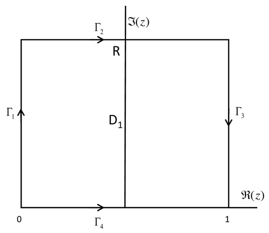
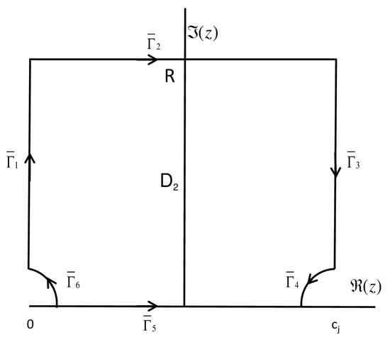
The functions $\frac{K(x_{n,j},x_l+th)e^{iwth}}{{(x_{n,j}-x_l-th)}^{\alpha }{(x_l+th)}^{\beta }}{L}_k\left(t\right)dt$ and $\frac{K(x_{n,j},x_n+th)e^{iwth}}{{(x_{n,j}-x_n-th)}^{\alpha }{(x_n+th)}^{\beta }}{L}_k\left(t\right)dt$ are analytic in the upper half-strip of complex planes $D_1$ and $D_2$, respectively, where region $D_1$ is enclosed by the curves ${\Gamma }_1,{\Gamma }_2,{\Gamma }_3,{\Gamma }_4$ and $D_2$ is enclosed by the curves ${\overline{\Gamma }}_1,{\overline{\Gamma }}_2,{\overline{\Gamma }}_3,{\overline{\Gamma }}_4,{\overline{\Gamma }}_5,{\overline{\Gamma }}_6$, as shown in Figure 1 and Figure 2, respectively. Then, based on the Cauchy theorem, we obtain

$$\begin{array}{cc}\hfill \tilde{I}\left[{\check{B}}_n^l\right]& =0,\hfill \\ \hfill \mathrm{where}\tilde{I}\left[{\check{B}}_n^l\right]& ={\int }_{{\Gamma }_1+{\Gamma }_2+{\Gamma }_3-{\Gamma }_4}\frac{K(x_{n,j},x_l+zh)e^{iwzh}}{{(x_{n,j}-x_l-zh)}^{\alpha }{(x_l+zh)}^{\beta }}{L}_k\left(z\right)dz,\hfill \end{array}$$

(12)

and

$$\begin{array}{cc}\hfill \tilde{I}\left[{\check{B}}_n\right]& =0,\hfill \\ \hfill \mathrm{where}\tilde{I}\left[{\check{B}}_n\right]& ={\int }_{{\overline{\Gamma }}_1+{\overline{\Gamma }}_2+{\overline{\Gamma }}_3+{\overline{\Gamma }}_4+{\overline{\Gamma }}_6-{\overline{\Gamma }}_5}\frac{K(x_{n,j},x_n+zh)e^{iwzh}}{{(x_{n,j}-x_n-zh)}^{\alpha }{(x_n+zh)}^{\beta }}{L}_k\left(z\right)dz,\hfill \end{array}$$

(13)

with the integration paths shown in Figure 1 and Figure 2 for (12) and (13), respectively.

Set ${\int }_{{\Gamma }_i}\frac{K(x_{n,j},x_l+zh)e^{iwzh}}{{(x_{n,j}-x_l-zh)}^{\alpha }{(x_l+zh)}^{\beta }}{L}_k\left(z\right)dz$ and ${\int }_{{\overline{\Gamma }}_j}\frac{K(x_{n,j},x_n+zh)e^{iwzh}}{{(x_{n,j}-x_n-zh)}^{\alpha }{(x_n+zh)}^{\beta }}{L}_k\left(z\right)dz$; we achieve

$$\begin{array}{cc}\hfill {\Gamma }_1+{\Gamma }_2+{\Gamma }_3-{\Gamma }_4& =0,\hfill \\ \hfill {\overline{\Gamma }}_1+{\overline{\Gamma }}_2+{\overline{\Gamma }}_3+{\overline{\Gamma }}_4+{\overline{\Gamma }}_6-{\overline{\Gamma }}_5& =0.\hfill \end{array}$$

(14)

For Equation (12), let $z=is$; then

$$\begin{array}{cc}\hfill {\Gamma }_1& =i{\int }_0^R\frac{K(x_{n,j},x_l+zh)e^{i\omega \left(is\right)h}}{{(x_{n,j}-x_l-\left(is\right)h)}^{\alpha }{(x_l+\left(is\right)h)}^{\beta }}{L}_k\left(is\right)ds,\hfill \\ \hfill {\Gamma }_1& =i{\int }_0^R\frac{K(x_{n,j},x_l+ish)e^{-\omega sh}}{{(x_{n,j}-x_l-ish)}^{\alpha }{(x_l+ish)}^{\beta }}{L}_k\left(is\right)ds.\hfill \end{array}$$

Similarly, for ${\Gamma }_3,z=1+is$, we have

$$\begin{array}{cc}\hfill {\Gamma }_3=& -i{\int }_0^R\frac{K(x_{n,j},x_l+(1+is)h)e^{i\omega (1+is)h}}{{(x_{n,j}-x_l-(1+is)h)}^{\alpha }{(x_l+(1+is)h)}^{\beta }}{L}_k(1+is)ds,\hfill \\ \hfill =& -i{e}^{i\omega h}{\int }_0^R\frac{K(x_{n,j},x_l+(1+is)h)e^{-\omega sh}}{{(x_{n,j}-x_l-(1+is)h)}^{\alpha }{(x_l+(1+is)h)}^{\beta }}{L}_k(1+is)ds.\hfill \end{array}$$

Now, for ${\Gamma }_2,z=s+iR$, we get

$$\begin{array}{cc}\hfill {\Gamma }_2=& {\int }_0^1\frac{K(x_{n,j},x_l+(s+iR)h)e^{i\omega (s+iR)h}}{{(x_{n,j}-x_l-(s+iR)h)}^{\alpha }{(x_l+(s+iR)h)}^{\beta }}{L}_k(s+iR)ds,\hfill \\ \hfill =& e^{-\omega Rh}{\int }_0^1\frac{K(x_{n,j},x_l+(s+iR)h)e^{i\omega sh}}{{(x_{n,j}-x_l-(s+iR)h)}^{\alpha }{(x_l+(s+iR)h)}^{\beta }}{L}_k(s+iR)ds\hfill \\ \hfill & {\Gamma }_2\to 0\mathrm{as}R\to \infty .\hfill \end{array}$$

It follows that

$$\begin{array}{cc}\hfill \tilde{I}\left[{\check{B}}_n^l\right]& =i{\int }_0^{\infty }\frac{K(x_{n,j},x_l+ish)e^{-\omega sh}}{{(x_{n,j}-x_l-ish)}^{\alpha }{(x_l+ish)}^{\beta }}{L}_k\left(is\right)ds\hfill \\ \hfill & -i{e}^{i\omega h}{\int }_0^{\infty }\frac{K(x_{n,j},x_l+(1+is)h)e^{-\omega sh}}{{(x_{n,j}-x_l-(1+is)h)}^{\alpha }{(x_l+(1+is)h)}^{\beta }}{L}_k(1+is)ds,\hfill \\ \hfill & =\frac{i}{\omega h}{\int }_0^{\infty }\frac{K(x_{n,j},x_l+\frac{it}{\omega })e^{-t}}{{(x_{n,j}-x_l-\frac{it}{\omega })}^{\alpha }{(x_l+\frac{it}{\omega })}^{\beta }}{L}_k\left(\frac{it}{\omega h}\right)dt\hfill \\ \hfill & -\frac{i}{\omega h}{e}^{i\omega h}{\int }_0^{\infty }\frac{K(x_{n,j},x_l+(h+\frac{it}{\omega }))e^{-t}}{{(x_{n,j}-x_l-(h+\frac{it}{\omega }))}^{\alpha }{(x_l+(h+\frac{it}{\omega }))}^{\beta }}{L}_k\left(1+\frac{it}{\omega h}\right)dt.\hfill \end{array}$$

(15)

Now applying the same procedure for Equation (13) and considering $z=is$, we obtain

$$\begin{array}{cc}\hfill {\overline{\Gamma }}_1& ={\int }_r^R\frac{K(x_{n,j},x_n+ish)e^{i\omega \left(is\right)h}}{{(x_{n,j}-x_n-ish)}^{\alpha }{(x_n+ish)}^{\beta }}{L}_k\left(is\right)ids,\hfill \\ \hfill & =i{\int }_r^R\frac{K(x_{n,j},x_n+ish)e^{-\omega sh}}{{(x_{n,j}-x_n-ish)}^{\alpha }{(x_n+ish)}^{\beta }}{L}_k\left(is\right)ds.\hfill \end{array}$$

Now for $z=c_j+is$, we have

$$\begin{array}{cc}\hfill {\overline{\Gamma }}_3& ={\int }_r^R\frac{K(x_{n,j},x_n+(c_j+is)h)e^{i\omega (c_j+is)h}}{{(x_{n,j}-x_n-(c_j+is)h)}^{\alpha }{(x_n+(c_j+is)h)}^{\beta }}{L}_k(c_j+is)ids,\hfill \\ \hfill & =i{e}^{i\omega c_{j}h}{\int }_r^R\frac{K(x_{n,j},x_n+(c_j+is)h)e^{-\omega sh}}{{(-ish)}^{\alpha }{(x_n+(c_j+is)h)}^{\beta }}{L}_k(c_j+is)ds,\hfill \\ \hfill & ={(-i)}^{1-\alpha }{h}^{-\alpha }{e}^{i\omega c_{j}h}{\int }_r^R\frac{K(x_{n,j},x_n+(c_j+is)h)e^{-\omega sh}}{{\left(s\right)}^{\alpha }{(x_n+(c_j+is)h)}^{\beta }}{L}_k(c_j+is)ds.\hfill \end{array}$$

Similarly,

$$\begin{array}{cc}\hfill {\overline{\Gamma }}_2& ={\int }_0^{c_j}\frac{K(x_{n,j},x_n+(s+iR)h)e^{i\omega (s+iR)h}}{{(x_{n,j}-x_n-(s+iR)h)}^{\alpha }{(x_n+(s+iR)h)}^{\beta }}{L}_k(s+iR)ds,\hfill \\ \hfill & =e^{-\omega Rh}{\int }_0^{c_j}\frac{K(x_{n,j},x_n+(s+iR)h)e^{i\omega s}}{{(x_{n,j}-x_n-(s+iR)h)}^{\alpha }{(x_n+(s+iR)h)}^{\beta }}{L}_k(s+iR)ds\hfill \\ \hfill & {\overline{\Gamma }}_2\to 0\mathrm{as}R\to \infty .\hfill \end{array}$$

Put $z=c_j+r{e}^{i\theta }$; we get

$$\begin{array}{cc}\hfill {\overline{\Gamma }}_4& =\left|ir{\int }_{\pi /2}^{\pi }\frac{K(x_{n,j},x_n+(c_j+r{e}^{i\theta })h)e^{i\omega (c_j+r{e}^{i\theta })h}}{{(x_{n,j}-x_n-(c_j+r{e}^{i\theta })h)}^{\alpha }{(x_n+(c_j+r{e}^{i\theta })h)}^{\beta }}{e}^{i\theta }{L}_k(c_j+r{e}^{i\theta })d\theta \right|,\hfill \\ \hfill & =\left|ir{e}^{i\omega c_{j}h}{\int }_{\pi /2}^{\pi }\frac{K(x_{n,j},x_n+(c_j+r{e}^{i\theta })h)e^{i\omega r{e}^{i\theta }h}}{{(-r{e}^{i\theta }h)}^{\alpha }{(x_n+(c_j+r{e}^{i\theta })h)}^{\beta }}{e}^{i\theta }{L}_k(c_j+r{e}^{i\theta })d\theta \right|,\hfill \\ \hfill & \le {\left|r\right|}^{1-\alpha }{\int }_{\pi /2}^{\pi }\left|\frac{K(x_{n,j},x_n+(c_j+r{e}^{i\theta })h)e^{i\omega r{e}^{i\theta }h}}{{(-e^{i\theta }h)}^{\alpha }{(x_n+(c_j+r{e}^{i\theta })h)}^{\beta }}{e}^{i\theta }{L}_k(c_j+r{e}^{i\theta })\right|d\theta \hfill \\ \hfill & \to 0\mathrm{as}r\to 0.\hfill \end{array}$$

Now, for $z=r{e}^{i\theta }$; we have

$$\begin{array}{cc}\hfill {\overline{\Gamma }}_6& =ir{\int }_{\pi /2}^{\pi }\frac{K(x_{n,j},x_n+r{e}^{i\theta }h)e^{i\omega h\left(r{e}^{i\theta }\right)}}{{(x_{n,j}-x_n-r{e}^{i\theta }h)}^{\alpha }{(x_n+r{e}^{i\theta }h)}^{\beta }}{e}^{i\theta }{L}_k\left(r{e}^{i\theta }\right)d\theta ,\hfill \\ \hfill & \le \left|r\right|{\int }_{\pi /2}^{\pi }\left|\frac{K(x_{n,j},x_n+r{e}^{i\theta }h)e^{i\omega h\left(r{e}^{i\theta }\right)}}{{(x_{n,j}-x_n-r{e}^{i\theta }h)}^{\alpha }{(x_n+r{e}^{i\theta }h)}^{\beta }}{e}^{i\theta }{L}_k\left(r{e}^{i\theta }\right)\right|d\theta \hfill \\ \hfill & \to 0\mathrm{as}r\to 0.\hfill \end{array}$$

It follows that

$$\begin{array}{cc}\hfill \tilde{I}\left[{\check{B}}_n\right]& =i{\int }_0^{\infty }\frac{K(x_{n,j},x_n+ish)e^{-\omega sh}}{{(x_{n,j}-x_n-ish)}^{\alpha }{(x_n+ish)}^{\beta }}{L}_k\left(is\right)ds\hfill \\ \hfill & +{(-i)}^{1-\alpha }{h}^{-\alpha }{e}^{i\omega c_{j}h}{\int }_0^{\infty }\frac{K(x_{n,j},x_n+(c_j+is)h)e^{-\omega sh}}{{\left(s\right)}^{\alpha }{(x_n+(c_j+is)h)}^{\beta }}{L}_k(c_j+is)ds,\hfill \\ \hfill & =\frac{i}{\omega h}{\int }_0^{\infty }\frac{K(x_{n,j},x_n+\frac{it}{\omega })e^{-t}}{{(x_{n,j}-x_n-\frac{it}{\omega })}^{\alpha }{(x_n+\frac{it}{\omega })}^{\beta }}{L}_k\left(\frac{it}{\omega h}\right)dt\hfill \\ \hfill & +{\left(\frac{-i}{\omega h}\right)}^{1-\alpha }{h}^{-\alpha }{e}^{i\omega c_{j}h}{\int }_0^{\infty }\frac{K(x_{n,j},x_n+c_{j}h+\frac{it}{\omega })e^{-t}}{{\left(\frac{t}{\omega h}\right)}^{\alpha }{(x_n+h{c}_j+\frac{it}{\omega })}^{\beta }}{L}_k\left(c_j+\frac{it}{\omega h}\right)dt.\hfill \end{array}$$

(16)

□

Furthermore, the Gauss–Laguerre quadrature and the generalized Gauss–Laguerre quadrature rules are applied to approximate the integrals (12) and (13). A convenient and straightforward method of generating Gaussian quadrature points and weights can be achieved with the $lagpts\left(n\right)$ function in the Chebfun system. For details, see [44].

3. Error Analysis

In this section, we perform some theoretical analysis. The solution’s asymptotic expression for (1) is provided by Theorem 2. Proposition 1 describes the error bound of the steepest descent method for highly oscillatory algebraic singular integrals. However, Theorem 3 gives the error bound for the collocation method proposed in this paper.

Theorem 2.

Let $y\left(x\right)$ be the solution of the highly oscillatory algebraic singular VIE (1) with $f\in C^m\left(I\right),K\in C^m\left(D\right)$ and $0<\alpha <1$. Then there exist functions $R_{\alpha ,j}^{\left(n\right)}$ and $S_{\alpha ,j}^{\left(n\right)}(j=0,1,\cdots ,m;n\ge 0)$ in $C^m\left(D\right)$ so that for $\omega \to \infty ,$ the solution has the asymptotic expansion

$$\begin{array}{cc}\hfill y\left(x\right)& =f\left(x\right)-(\frac{1}{i\omega }{)}^m\sum _{n=1}^{\infty }{\int }_0^x{(x-t)}^{n(1-\alpha )-1}{t}^{-\beta }{S}_{(1-\alpha ),m}^{\left(n\right)}(x,t)e^{i\omega (x-t)}dt\hfill \\ \hfill & -\sum _{j=0}^{m-1}(\frac{1}{i\omega }{)}^{j+1}\sum _{n=1}^{\infty }{S}_{(1-\alpha ),j}^{\left(n\right)}(x,x){\int }_0^x{t}^{-\beta }{(x-t)}^{n(1-\alpha )-1}{e}^{iw(x-t)}dt,\hfill \end{array}$$

(17)

where the infinite series converges absolutely and uniformly on I. The meaning of $R_{\alpha ,j}^{\left(n\right)}$ and $S_{\alpha ,j}^{\left(n\right)}$ is defined clearly in the proof.

Proof. 

According to [20] the unique solution of (1) with $\beta =0$ is given as

$$y\left(x\right)=f\left(x\right)-{\int }_0^x{(x-t)}^{-\alpha }\sum _{n=1}^{\infty }{(x-t)}^{(n-1)(1-\alpha )}{\psi }_{(1-\alpha ),n}(x,t)e^{i\omega (x-t)}f\left(t\right)dt,$$

which can be further extended for $\beta \ne 0$ as

$$y\left(x\right)=f\left(x\right)-{\int }_0^x{(x-t)}^{-\alpha }{t}^{-\beta }\sum _{n=1}^{\infty }{(x-t)}^{(n-1)(1-\alpha )}{\psi }_{(1-\alpha ),n}(x,t)e^{i\omega (x-t)}f\left(t\right)dt,$$

(18)

where ${\psi }_{(1-\alpha ),n}\in C^m\left(D\right)$ and ${\psi }_{(1-\alpha ),1}(x,t)=K(x,t).$ Owing to the presence of the singular (non-smooth) terms ${(x-t)}^{-\alpha }{(x-t)}^{(n-1)(1-\alpha )}={(x-t)}^{n(1-\alpha )-1}$, the process of subtraction of the singularity is followed as:

Let $S_{(1-\alpha ),n}^{\left(0\right)}(x,t)={\psi }_{(1-\alpha ),n}(x,t)f\left(t\right)$, then

$$S_{(1-\alpha ),n}^{\left(0\right)}(x,t)=(S_{(1-\alpha ),n}^{\left(0\right)}(x,t)-S_{(1-\alpha ),n}^{\left(0\right)}(x,x))+S_{(1-\alpha ),n}^{\left(0\right)}(x,x).$$

(19)

Since $S_{(1-\alpha ),n}^{\left(0\right)}\in C^m\left(D\right)$, the application of Taylor’s theorem directs to

$$\begin{array}{cc}\hfill S_{(1-\alpha ),n}^{\left(0\right)}(x,t)-S_{(1-\alpha ),n}^{\left(0\right)}(x,x)& =\sum _{j=1}^q\frac{{(-1)}^j}{j!}\frac{{\partial }^j{S}_{(1-\alpha ),n}^{\left(0\right)}(x,x)}{\partial t^j}{(x-t)}^j+(x-t){\zeta }_{m-1,n}^{\left(0\right)}(x,t),\hfill \\ \hfill & =(x-t)\sum _{j=1}^q\frac{{(-1)}^j}{j!}\frac{{\partial }^j{S}_{(1-\alpha ),n}^{\left(0\right)}(x,x)}{\partial t^j}{(x-t)}^{j-1}+{\zeta }_{m-1,n}^{\left(0\right)}(x,t),\hfill \\ \hfill & =(x-t)R_{(1-\alpha ),n}^{\left(0\right)}(x,t).\hfill \end{array}$$

Thus, the solution $y\in I$ can be written as

$$\begin{array}{cc}\hfill y\left(x\right)& =f\left(x\right)-\sum _{n=1}^{\infty }{\int }_0^x{(x-t)}^{n(1-\alpha )-1}{t}^{-\beta }((x-t)R_{(1-\alpha ),n}^{\left(0\right)}(x,t)+S_{(1-\alpha ),n}^{\left(0\right)}(x,x))e^{iw(x-t)}dt,\hfill \\ \hfill & =f\left(x\right)-\sum _{n=1}^{\infty }{\int }_0^x{(x-t)}^{n(1-\alpha )}{t}^{-\beta }{R}_{(1-\alpha ),n}^{\left(0\right)}(x,t)e^{iw(x-t)}dt\hfill \\ \hfill & -\sum _{n=1}^{\infty }{S}_{(1-\alpha ),n}^{\left(0\right)}(x,x){\int }_0^x{t}^{-\beta }{(x-t)}^{n(1-\alpha )-1}{e}^{iw(x-t)}dt.\hfill \end{array}$$

To solve the first integral in the above equation containing $R_{(1-\alpha ),n}^{\left(0\right)}(x,t)$, integration by parts can be applied as

$$\begin{array}{cc}\hfill & {\int }_0^x{(x-t)}^{n(1-\alpha )}{t}^{-\beta }{R}_{(1-\alpha ),n}^{\left(0\right)}(x,t)e^{iw(x-t)}dt\hfill \\ \hfill & ={\int }_0^x{(x-t)}^{n(1-\alpha )}{t}^{-\beta }{R}_{(1-\alpha ),n}^{\left(0\right)}(x,t)(-\frac{1}{i\omega }\frac{\partial e^{iw(x-t)}}{\partial t}dt),\hfill \\ \hfill & =\frac{1}{i\omega }({\int }_0^x-n(1-\alpha ){(x-t)}^{n(1-\alpha )-1}{t}^{-\beta }{R}_{(1-\alpha ),n}^{\left(0\right)}(x,t)e^{iw(x-t)}dt\hfill \\ \hfill & +{\int }_0^x{(x-t)}^{n(1-\alpha )}{t}^{-\beta }\frac{\partial R_{(1-\alpha ),n}^{\left(0\right)}(x,t)}{\partial t}{e}^{iw(x-t)}dt\hfill \\ \hfill & +{\int }_0^x-\beta {(x-t)}^{n(1-\alpha )}{t}^{-\beta -1}{R}_{(1-\alpha ),n}^{\left(0\right)}(x,t)e^{iw(x-t)}dt),\hfill \\ \hfill & =\frac{1}{i\omega }{\int }_0^x{(x-t)}^{n(1-\alpha )-1}{t}^{-\beta }{S}_{(1-\alpha ),n}^{\left(1\right)}(x,t)e^{i\omega (x-t)}dt.\hfill \end{array}$$

(20)

It follows that

$$\begin{array}{cc}\hfill y\left(x\right)& =f\left(x\right)-\sum _{n=1}^{\infty }\frac{1}{i\omega }{\int }_0^x{(x-t)}^{n(1-\alpha )-1}{t}^{-\beta }{S}_{(1-\alpha ),n}^{\left(1\right)}(x,t)e^{i\omega (x-t)}dt\hfill \\ \hfill & -\sum _{n=1}^{\infty }{S}_{(1-\alpha ),n}^{\left(0\right)}(x,x){\int }_0^x{t}^{-\beta }{(x-t)}^{n(1-\alpha )-1}{e}^{iw(x-t)}dt.\hfill \end{array}$$

Thus, by considering (19) in order to subtract the singularity from the integral involving $S_{(1-\alpha ),n}^{\left(1\right)}(x,t)$, the proof is proved by induction. □

Proposition 1.

Suppose that $y\left(z\right)$ is a function that is analytic in the half-strip of the complex plane $a\le \Re \left(z\right)\le b$ and $\Im \left(z\right)\ge 0$ and which satisfies:

$$\begin{array}{cc}\hfill & {\int }_0^1\left|y(z+iR)\right|dz\le M{R}^{\alpha +\beta }{e}^{{\omega }_{0}R},0<{\omega }_0<\omega ,\hfill \\ \hfill & {\int }_0^{c_j}\left|y(z+iR)\right|dz\le M{R}^{\alpha +\beta }{e}^{{\omega }_{0}R},0<{\omega }_0<\omega ;\hfill \end{array}$$

then the error for the method described in (10) is defined as $E\left[{\check{B}}_n^l\right]=|I\left[{\check{B}}_n^l\right]-\tilde{I}\left[{\check{B}}_n^l\right]|$ and $E\left[{\check{B}}_n\right]=|I\left[{\check{B}}_n\right]-\tilde{I}\left[{\check{B}}_n\right]|$, respectively, where

$$\begin{array}{cc}\hfill E\left[{\check{B}}_n^l\right]=& O\left(\frac{{(l!)}^2}{\left(2l\right)!{\omega }^{2l+1}h}\right),\hfill \\ \hfill E\left[{\check{B}}_n\right]=& O\left(\frac{l!}{\left(2l\right)!h}\right[min(\frac{l!}{{\omega }^{2l+1}},\frac{\Gamma (-\alpha +l+1)}{{\omega }^{1-\alpha +2l}}).\hfill \end{array}$$

(21)

Proof. 

The error formula for the l-point Gauss–Laguerre quadrature rule for ${\int }_0^{+\infty }y\left(t\right)e^{-t}dt$ is defined as

$$\frac{{(l!)}^2}{\left(2l\right)!}{y}^{\left(2l\right)}\left(\zeta \right),0<\zeta <+\infty .$$

(22)

Also, for the integral ${\int }_0^{+\infty }y\left(t\right)t^{\nu }{e}^{-t}dt,\nu >-1$, the error formula for the $l—$point generalized Gauss–Laguerre quadrature rule is defined as [45]

$$\frac{l!\Gamma (l+\nu +1)}{\left(2l\right)!}{y}^{\left(2l\right)}\left(\zeta \right),0<\zeta <+\infty .$$

(23)

By using Formula (22), we yield

$$\begin{array}{cc}\hfill E\left[{\check{B}}_n^l\right]& \le \frac{{(l!)}^2}{\left(2l\right)!\omega h}\left|\right[\frac{K(x_{n,j},x_l+\frac{it}{\omega })}{{(x_{n,j}-x_l-\frac{it}{\omega })}^{\alpha }{(x_l+\frac{it}{\omega })}^{\beta }}y\left(\frac{it}{\omega h}\right){]}_{{\zeta }_1}^{\left(2l\right)}|\hfill \\ \hfill & +\frac{{(l!)}^2}{\left(2l\right)!\omega h}\left|\right[\frac{K(x_{n,j},x_l+(h+\frac{it}{\omega }))}{{(x_{n,j}-x_l-(h+\frac{it}{\omega }))}^{\alpha }{(x_l+(h+\frac{it}{\omega }))}^{\beta }}y\left(1+\frac{it}{\omega h}\right){]}_{{\zeta }_2}^{\left(2l\right)}|,\hfill \\ \hfill & =\frac{{(l!)}^2}{\left(2l\right)!{\omega }^{2l+1}h}\left|\right[\frac{K(x_{n,j},x_l+i{\xi }_1)}{{(x_{n,j}-x_l-i{\xi }_1)}^{\alpha }{(x_l+i{\xi }_1)}^{\beta }}y\left(\frac{i{\xi }_1}{h}\right){]}_{{\xi }_1={\zeta }_1/\omega }^{\left(2l\right)}|\hfill \\ \hfill & +\frac{{(l!)}^2}{\left(2l\right)!{\omega }^{2l+1}h}\left|\right[\frac{K(x_{n,j},x_l+(h+i{\xi }_2))}{{(x_{n,j}-x_l-(h+i{\xi }_2))}^{\alpha }{(x_l+(h+i{\xi }_2))}^{\beta }}y\left(1+\frac{i{\xi }_2}{h}\right){]}_{{\xi }_2={\zeta }_2/\omega }^{\left(2l\right)}|,\hfill \\ \hfill & =O\left(\frac{{(l!)}^2}{\left(2l\right)!{\omega }^{2l+1}h}\right).\hfill \end{array}$$

For $E\left[{\check{B}}_n\right]$, again, by using Formulas (22) and (23), we get

$$\begin{array}{cc}\hfill E\left[{\check{B}}_n\right]& \le \frac{{(l!)}^2}{\left(2l\right)!\omega h}\left|\right[\frac{K(x_{n,j},x_n+\frac{it}{\omega })}{{(x_{n,j}-x_n-\frac{it}{\omega })}^{\alpha }{(x_n+\frac{it}{\omega })}^{\beta }}y\left(\frac{it}{\omega h}\right){]}_{{\zeta }_3}^{\left(2l\right)}|\hfill \\ \hfill & +\frac{l!\Gamma (-\alpha +l+1)}{\left(2l\right)!{\omega }^{1-\alpha }h}\left|\right[\frac{K(x_{n,j},x_n+c_{j}h+\frac{it}{\omega }))}{{(x_n+c_{j}h+\frac{it}{\omega })}^{\beta }}y\left(c_j+\frac{it}{\omega h}\right){]}_{{\zeta }_4}^{\left(2l\right)}|,\hfill \\ \hfill & =\frac{{(l!)}^2}{\left(2l\right)!{\omega }^{2l+1}h}\left|\right[\frac{K(x_{n,j},x_n+i{\xi }_3)}{{(x_{n,j}-x_n-\frac{it}{\omega })}^{\alpha }{(x_n+i{\xi }_3)}^{\beta }}y\left(\frac{i{\xi }_3}{h}\right){]}_{{\xi }_3={\zeta }_3/\omega }^{\left(2l\right)}|\hfill \\ \hfill & +\frac{l!\Gamma (-\alpha +l+1)}{\left(2l\right)!{\omega }^{1-\alpha +2l}h}\left|\right[\frac{K(x_{n,j},x_n+c_{j}h+i{\xi }_4))}{{(x_n+c_{j}h+i{\xi }_4)}^{\beta }}y\left(c_j+\frac{i{\xi }_4}{h}\right){]}_{{\xi }_4={\zeta }_4/\omega }^{\left(2l\right)}|,\hfill \\ \hfill & =O\left(\frac{l!}{\left(2l\right)!h}\right[min(\frac{l!}{{\omega }^{2l+1}},\frac{\Gamma (-\alpha +l+1)}{{\omega }^{1-\alpha +2l}}).\hfill \end{array}$$

(24)

□

Theorem 3.

Suppose that function $f\left(x\right)\in C^m\left([0,1]\right)$ and $K(x,t)\in C^m([0,1]\times [0,1])$; then, by considering Theorem 3.2 in [40], the numerical solution defined by (8) satisfies

$$sup|y\left(x\right)-y_h\left(x\right)|\le Cmax\left\{min(\frac{1}{{\omega }^{1-\alpha -\beta }},h^{1-\alpha }),h^m\right\};$$

(25)

here, C is a constant that is independent of h and ω.

4. Numerical Examples

This current section is dedicated to presenting the efficiency of the proposed method. The exact values are obtained from Mathematica 11, whereas MATLAB R2023a is used to compute the results by applying the proposed method. In some examples, the exact values are calculated by taking sufficiently large values of N by the proposed method. The absolute error is calculated as $|y\left(x_j\right)-\tilde{y}\left(x_j\right)|$, where $\tilde{y}\left(x_j\right)$ represents the approximated solution, and the exact solution is defined by $y\left(x_j\right)$. The numerical results computed by the PCCM and the PLCM are presented as follows:

Example 1.

Considering $f\left(x\right)=e^x,\alpha =0.5$ and $\beta =0.1,0.2$,

Table 1. The absolute error for $\omega ={10}^3,\alpha =0.5,$ and $\beta =0.2$.

Method	$\mathit{N}$	$|\mathit{y}\left({\mathit{x}}_{\mathit{j}}\right)-\tilde{\mathit{y}}\left({\mathit{x}}_{\mathit{j}}\right)|$
PLCM	10	5.01836 $\times {10}^{-3}$
PCCM	10	4.55659 $\times {10}^{-3}$
PLCM	100	5.98446 $\times {10}^{-3}$
PCCM	100	5.39355 $\times {10}^{-3}$
PLCM	1000	5.27239 $\times {10}^{-4}$
PCCM	1000	8.07002 $\times {10}^{-4}$

,

Table 2. The absolute error for $\omega ={10}^4$, $\alpha =0.5,$ and $\beta =0.1$.

Method	$\mathit{N}$	$|\mathit{y}\left({\mathit{x}}_{\mathit{j}}\right)-\tilde{\mathit{y}}\left({\mathit{x}}_{\mathit{j}}\right)|$
PLCM	100	3.18340 $\times {10}^{-4}$
PCCM	100	1.85657 $\times {10}^{-4}$
PLCM	1000	2.24953 $\times {10}^{-4}$
PCCM	1000	5.28067 $\times {10}^{-5}$

,

Table 3. The absolute error for $\omega ={10}^5$, $\alpha =0.5,$ and $\beta =0.1$.

Method	$\mathit{N}$	$|\mathit{y}\left({\mathit{x}}_{\mathit{j}}\right)-\tilde{\mathit{y}}\left({\mathit{x}}_{\mathit{j}}\right)|$
PLCM	100	3.18605 $\times {10}^{-5}$
PCCM	100	1.31605 $\times {10}^{-5}$
PLCM	1000	3.59854 $\times {10}^{-5}$
PCCM	1000	1.69869 $\times {10}^{-5}$

,

Table 4. The absolute error for $\omega ={10}^6$, $\alpha =0.5,$ and $\beta =0.1$.

Method	$\mathit{N}$	$|\mathit{y}\left({\mathit{x}}_{\mathit{j}}\right)-\tilde{\mathit{y}}\left({\mathit{x}}_{\mathit{j}}\right)|$
PLCM	100	8.40761 $\times {10}^{-6}$
PCCM	100	8.40761 $\times {10}^{-6}$
PLCM	1000	3.59636 $\times {10}^{-8}$
PCCM	1000	9.77366 $\times {10}^{-6}$

and

Table 5. The exact and approximated values for $\omega ={10}^7,\alpha =0.5,\beta =0.1,$ and $N=1000$.

x	Method	$\tilde{\mathit{y}}\left({\mathit{x}}_{\mathit{j}}\right)$	$\mathit{y}\left({\mathit{x}}_{\mathit{j}}\right)$	$|\mathit{y}\left({\mathit{x}}_{\mathit{j}}\right)-\tilde{\mathit{y}}\left({\mathit{x}}_{\mathit{j}}\right)|$
0.4	PLCM	1.491177522505289–9.000647139899675i	1.491177506337760–0.000647192209957i	5.47517 $\times {10}^{-8}$
0.4	PCCM	1.491177505908644–4.000647190817211i	1.491177652328156–6.000647075941965i	1.86104 $\times {10}^{-7}$
0.7	PLCM	2.012926085893602–2.000826801897145i	2.012926065551880–0.000826867858290i	6.90265 $\times {10}^{-8}$
0.7	PCCM	2.012926249972612–2.000826813578346i	2.012926064180901–1.000826866108774i	1.93075 $\times {10}^{-7}$

show the absolute error for the equation

$$y\left(x\right)+{\int }_0^x\frac{K(x,t)e^{i\omega (x-t)}}{{(x-t)}^{\alpha }{t}^{\beta }}y\left(t\right)dt=f\left(x\right),x\in [0,1].$$

(26)

Then, the exact solution for $y\left(x\right)$ can be written as

$$y\left(x\right)=f\left(x\right)+{\int }_0^x{R}_{\alpha }(x,t)e^{i\omega (x-t)}f\left(t\right)dt,$$

where $R_{\alpha }(x,t)$ is defined as

$$R_{\alpha }(x,t)=t^{-\beta }\sum _{n=1}^{\infty }\frac{{(-\Gamma (1-\alpha ))}^n}{\Gamma \left(n\right(1-\alpha \left)\right)}{(x-t)}^{(n-n\alpha -1).}$$

(27)

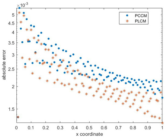
For further details, see [20]. Based on Table 1, Table 2, Table 3, Table 4 and Table 5, it can be seen that the PCCM and the PLCM provide high-precision accuracy rates as w increases. Additionally, Figure 3 shows the absolute error for the PCCM and the PLCM with $\alpha =0.5,\beta =0.1,$ and $\omega ={10}^3.$

The accuracy of the numerical methods presented in this paper is compared with the results claimed in [43] on a uniform mesh for (26) with $f\left(x\right)=e^x,\alpha =0.1,$ and $\beta =0$.

Table 6. The comparison of PCCM and PLCM for $N=5$ with $U_{10}^{L,0}$ and $U_{10}^{L,1}$ [43].

$\mathit{\omega }$	${\mathit{U}}_{10}^{\mathit{L},0}$	${\mathit{U}}_{10}^{\mathit{L},1}$	PCCM	PLCM
1	2.81 $\times {10}^{-2}$	9.99 $\times {10}^{-4}$	2.17 $\times {10}^{-2}$	1.63 $\times {10}^{-2}$
${10}^2$	8.74 $\times {10}^{-3}$	6.50 $\times {10}^{-3}$	8.24 $\times {10}^{-3}$	4.18 $\times {10}^{-3}$
${10}^4$	1.02 $\times {10}^{-4}$	6.94 $\times {10}^{-5}$	3.99 $\times {10}^{-5}$	3.82 $\times {10}^{-5}$
${10}^8$	8.59 $\times {10}^{-9}$	6.94 $\times {10}^{-9}$	3.90 $\times {10}^{-9}$	7.07 $\times {10}^{-9}$

following explains that for $\omega \gg 1$, the results presented in [43] for $N=10$ can be obtained by applying the PCCM and the PLCM for $N=5$.

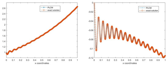
Figure 4 and Figure 5 illustrate the exact solution and numerical solutions computed by the PCCM and the PLCM. As can be seen in the figures below, the solution exhibits a singularity and oscillatory behavior. With increasing ω, increasing oscillation is observed in the imaginary part of the solution.

Example 2.

For $f\left(x\right)=sin\left(x\right),\alpha =0.5,$ and $\beta =0.2,0.1$,

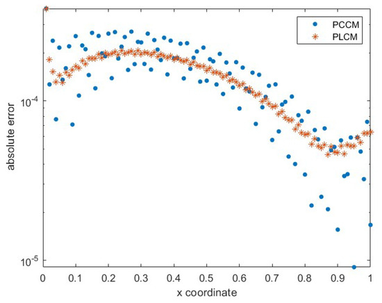
Table 7. The absolute error for $\omega ={10}^3$, $\alpha =0.5,$ and $\beta =0.2$.

Method	$\mathit{N}$	$|\mathit{y}\left({\mathit{x}}_{\mathit{j}}\right)-\tilde{\mathit{y}}\left({\mathit{x}}_{\mathit{j}}\right)|$
PLCM	10	4.48905 $\times {10}^{-4}$
PCCM	10	8.47592 $\times {10}^{-4}$
PLCM	100	1.27823 $\times {10}^{-4}$
PCCM	100	1.04778 $\times {10}^{-4}$
PLCM	1000	1.85025 $\times {10}^{-4}$
PCCM	1000	7.15488 $\times {10}^{-3}$

,

Table 8. The absolute error for $\omega ={10}^4$, $\alpha =0.5,$ and $\beta =0.1$.

Method	$\mathit{N}$	$|\mathit{y}\left({\mathit{x}}_{\mathit{j}}\right)-\tilde{\mathit{y}}\left({\mathit{x}}_{\mathit{j}}\right)|$
PLCM	100	1.67841 $\times {10}^{-5}$
PCCM	100	1.96906 $\times {10}^{-5}$
PLCM	1000	7.10459 $\times {10}^{-6}$
PCCM	1000	7.55101 $\times {10}^{-6}$

,

Table 9. The absolute error for $\omega ={10}^5$, $\alpha =0.5,$ and $\beta =0.1$.

Method	$\mathit{N}$	$|\mathit{y}\left({\mathit{x}}_{\mathit{j}}\right)-\tilde{\mathit{y}}\left({\mathit{x}}_{\mathit{j}}\right)|$
PLCM	100	1.58367 $\times {10}^{-6}$
PCCM	100	1.41486 $\times {10}^{-6}$
PLCM	1000	1.19504 $\times {10}^{-6}$
PCCM	1000	1.05706 $\times {10}^{-6}$

,

Table 10. The absolute error for $\omega ={10}^6$, $\alpha =0.5,$ and $\beta =0.1$.

Method	$\mathit{N}$	$|\mathit{y}\left({\mathit{x}}_{\mathit{j}}\right)-\tilde{\mathit{y}}\left({\mathit{x}}_{\mathit{j}}\right)|$
PLCM	100	1.17697 $\times {10}^{-7}$
PCCM	100	1.90615 $\times {10}^{-7}$
PLCM	1000	6.73424 $\times {10}^{-8}$
PCCM	1000	1.31592 $\times {10}^{-7}$

and

Table 11. The absolute error for $\omega ={10}^7$, $\alpha =0.5,$ and $\beta =0.1$.

Method	$\mathit{N}$	$|\mathit{y}\left({\mathit{x}}_{\mathit{j}}\right)-\tilde{\mathit{y}}\left({\mathit{x}}_{\mathit{j}}\right)|$
PLCM	100	1.14208 $\times {10}^{-8}$
PCCM	100	2.62249 $\times {10}^{-8}$
PLCM	1000	5.39604 $\times {10}^{-9}$
PCCM	1000	7.21998 $\times {10}^{-9}$

show the absolute error for the equation

$$y\left(x\right)+{\int }_0^x\frac{K(x,t)e^{i\omega (x-t)}}{{(x-t)}^{\alpha }{t}^{\beta }}y\left(t\right)dt=f\left(x\right),x\in [0,1].$$

(28)

The exact solution for y(x) can be written as

$$y\left(x\right)=f\left(x\right)+{\int }_0^x{R}_{\alpha }(x,t)e^{i\omega (x-t)}f\left(t\right)dt,$$

where $R_{\alpha }(x,t)$ is defined as (27). It is evident from Table 7, Table 8, Table 9, Table 10 and Table 11 that the PCCM and the PLCM provide high-precision accuracy rates as w increases. Further, Figure 6 shows the absolute errors for the PCCM and the PLCM with $\alpha =0.5,\beta =0.2,$ and $\omega ={10}^3.$

Example 3.

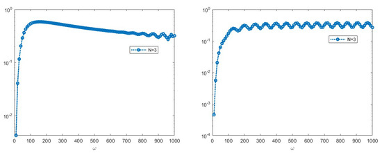
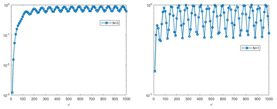
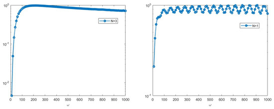
The following example proves the accuracy of the error-bound claimed in Proposition (1) for $E\left[{\check{B}}_n^l\right]$ and $E\left[{\check{B}}_n\right]$ calculated by the steepest descent method followed by Theorem 1. Figure 7, Figure 8 and Figure 9 show the scaled absolute errors for $I\left[{\check{B}}_n^l\right]$ and $I\left[{\check{B}}_n\right]$ with different values of $\alpha ,\beta ,N,$ and ω from 10 to 1000.

5. Conclusions

The purpose of this paper is to propose and illustrate an efficient and effective method for solving highly oscillatory algebraic singular VIEs. Based on the application of the proposed PCCM and PLCM, it has been verified that both methods yield nearly identical approximate results for highly oscillatory algebraic singular integral variables. We have demonstrated that the proposed method delivers satisfactory results even when the number of $\omega$ increases. In Table 6, it has been proved that the PCCM and PLCM can obtain the required exact accuracy for smaller values of N when compared with the method presented in [43]. Moreover, the scaled absolute error graphs also provide evidence of the efficiency and validity of the convergence rate for the highly oscillatory algebraic singular integrals $I\left[{\check{B}}_n^l\right]$ and $I\left[{\check{B}}_n\right]$.

However, in this paper, we have considered the highly oscillatory algebraic singular VIEs, and in future work, the PCCM and PLCM proposed in this paper can be used and modified accordingly to solve algebraic singular VIEs with highly oscillatory Bassel kernel functions.

References

- Colton, D.L.; Kress, R.; Kress, R. Inverse Acoustic and Electromagnetic Scattering Theory, 2nd ed.; Springer: New York City, NY, USA, 1998. [Google Scholar]
- Nédélec, J.C. Acoustic and Electromagnetic Equations: Integral Representations for Harmonic Problems, 1st ed.; Springer: New York City, NY, USA, 2001. [Google Scholar]
- Pike, E.R.; Sabatier, P.C. (Eds.) Scattering, Two-Volume Set: Scattering and Inverse Scattering in Pure and Applied Science, 1st ed.; Academic Press: London, UK, 2001. [Google Scholar]
- Ali, A.H. Applications of differential transform method to initial value problems. Am. J. Eng. Res. 2017, 6, 365–371. [Google Scholar]
- Abu-Ghuwaleh, M.; Saadeh, R.; Qazza, A. General master theorems of integrals with applications. Mathematics 2022, 10, 3547. [Google Scholar] [CrossRef]
- Adomian, G. Solving Frontier Problems of Physics: The Decomposition Method, 1st ed.; Springer: New York City, NY, USA, 2013. [Google Scholar]
- Atkinson, K.E. The Numerical Solution of Integral Equations of the Second Kind; Cambridge University Press: Cambridge, UK, 1997. [Google Scholar]
- Suslov, K.; Gerasimov, D.; Solodusha, S. Smart grid: Algorithms for control of active-adaptive network components. In Proceedings of the 2015 IEEE Eindhoven PowerTech, Eindhoven, The Netherlands, 29 June–2 July 2015; pp. 1–6. [Google Scholar]
- Fomin, O.; Masri, M.; Pavlenko, V. Intelligent technology of nonlinear dynamics diagnostics using Volterra kernels moments. Int. J. Math. Models Methods Appl. Sci. 2016, 10, 158–165. [Google Scholar]
- Ma, W.X.; Huang, Y.; Wang, F. Inverse scattering transforms for non-local reverse-space matrix non-linear Schrödinger equations. Eur. J. Appl. Math. 2022, 33, 1062–1082. [Google Scholar] [CrossRef]
- Wazwaz, A.M. Linear and Nonlinear Integral Equations, 1st ed.; Springer: New York City, NY, USA, 2011. [Google Scholar]
- Jerri, A.J. Introduction to Integral Equations with Applications, 2nd ed.; Wiley-Interscience: Hoboken, NJ, USA, 1999. [Google Scholar]
- Willis, J.R.; Nemat-Nasser, S. Singular perturbation solution of a class of singular integral equations. Q. Appl. Math. 1990, 48, 741–753. [Google Scholar] [CrossRef][Green Version]
- Solodusha, S.; Bulatov, M. Integral equations related to volterra series and inverse problems: Elements of theory and applications in heat power engineering. Mathematics 2021, 9, 1905. [Google Scholar] [CrossRef]
- Brunner, H. On the numerical solution of first-kind Volterra integral equations with highly oscillatory kernels. In Proceedings of the INI. HOP., Cambridge, UK, 13–17 September 2010. [Google Scholar]
- Zakęś, F.; Śniady, P. Application of Volterra integral equations in dynamics of multispan uniform continuous beams subjected to a moving load. Shock. Vib. 2016, 2016, 4070627. [Google Scholar] [CrossRef]
- Asheim, A.; Huybrechs, D. Local solutions to high-frequency 2D scattering problems. J. Comput. Phys. 2010, 229, 5357–5372. [Google Scholar] [CrossRef]
- Langdon, S.; Chandler-Wilde, S.N. A wavenumber independent boundary element method for an acoustic scattering problem. SIAM J. Numer. Anal. 2006, 43, 2450–2477. [Google Scholar] [CrossRef]
- Colton, D.; Kress, R. Integral Equation Methods in Scattering Theory; SIAM: Philadelphia, PA, USA, 2013. [Google Scholar]
- Brunner, H. Volterra Integral Equations: An Introduction to Theory and Applications, 1st ed.; Cambridge University Press: Cambridge, UK, 2017. [Google Scholar]
- Polyanin, P.; Manzhirov, A.V. Handbook of Integral Equations, 2nd ed.; Chapman and Hall/CRC: Boca Raton, FL, USA, 2008. [Google Scholar]
- Odibat, Z.M. Differential transform method for solving Volterra integral equation with separable kernels. Math. Comput. Model. 2008, 48, 1144–1149. [Google Scholar] [CrossRef]
- Hetmaniok, E.; Pleszczyński, M.; Khan, Y. Solving the Integral Differential Equations with Delayed Argument by Using the DTM Method. Sensors 2022, 22, 4124. [Google Scholar] [CrossRef] [PubMed]
- Hetmaniok, E.; Pleszczyński, M. Comparison of the Selected Methods Used for Solving the Ordinary Differential Equations and Their Systems. Mathematics 2022, 10, 306. [Google Scholar] [CrossRef]
- Xiang, S. Efficient Filon-type methods for ∫abf(x)eiωg(x)dx. Numer. Math. 2007, 105, 633–658. [Google Scholar] [CrossRef]
- Zaman, S. Meshless procedure for highly oscillatory kernel based one-dimensional Volterra integral equations. J. Comput. Appl. Math. 2022, 413, 114360. [Google Scholar]
- Kant, K.; Nelakanti, G. Approximation methods for second kind weakly singular Volterra integral equations. J. Comput. Appl. Math. 2020, 368, 112531. [Google Scholar] [CrossRef]
- Zhu, L.; Wang, Y. Numerical solutions of Volterra integral equation with weakly singular kernel using SCW method. Appl. Math. Comput. 2015, 260, 63–70. [Google Scholar] [CrossRef]
- Brunner, H. Collocation Methods for Volterra Integral and Related Functional Differential Equations; Cambridge University Press: Cambridge, UK, 2004. [Google Scholar]
- Chen, Y.; Tang, T. Convergence analysis of the Jacobi spectral-collocation methods for Volterra integral equations with a weakly singular kernel. Math. Comput. 2010, 79, 147–167. [Google Scholar] [CrossRef]
- Li, X.; Tang, T. Convergence analysis of Jacobi spectral collocation methods for Abel-Volterra integral equations of second kind. Front. Math. China 2012, 7, 69–84. [Google Scholar] [CrossRef]
- Chen, Y.; Tang, T. Spectral methods for weakly singular Volterra integral equations with smooth solutions. J. Comput. Appl. Math. 2009, 233, 938–950. [Google Scholar] [CrossRef]
- Talaei, Y. Chelyshkov collocation approach for solving linear weakly singular Volterra integral equations. J. Appl. Math. Comput. 2019, 60, 201–222. [Google Scholar] [CrossRef]
- Ma, J.; Xiang, S. A collocation boundary value method for linear Volterra integral equations. J. Sci. Comput. 2017, 71, 1–20. [Google Scholar] [CrossRef]
- Xiang, S.; Brunner, H. Efficient methods for Volterra integral equations with highly oscillatory Bessel kernels. BIT Numer. Math. 2013, 53, 241–263. [Google Scholar] [CrossRef]
- Fang, C.; He, G.; Xiang, S. Hermite-type collocation methods to solve volterra integral equations with highly oscillatory Bessel kernels. Symmetry 2019, 11, 168. [Google Scholar] [CrossRef]
- Fermo, L.; Occorsio, D. Weakly singular linear Volterra integral equations: A Nyström method in weighted spaces of continuous functions. J. Comput. Appl. Math. 2022, 406, 114001. [Google Scholar] [CrossRef]
- Li, X.; Tang, T.; Xu, C. Numerical solutions for weakly singular Volterra integral equations using Chebyshev and Legendre pseudo-spectral Galerkin methods. J. Sci. Comput. 2016, 67, 43–64. [Google Scholar] [CrossRef]
- Wang, T.; Lian, H.; Ji, L. Singularity separation Chebyshev collocation method for weakly singular Volterra integral equations of the second kind. Numer. Algorithms 2023, 2023, 1–26. [Google Scholar] [CrossRef]
- Wu, Q.; Sun, M. On the convergence rate of collocation methods for Volterra integral equations with weakly singular oscillatory trigonometric kernels. Results Appl. Math. 2023, 17, 100352. [Google Scholar] [CrossRef]
- Xiang, S.; Wu, Q. Numerical solutions to Volterra integral equations of the second kind with oscillatory trigonometric kernels. Appl. Math. Comput. 2013, 223, 34–44. [Google Scholar] [CrossRef]
- Liang, H.; Brunner, H. The fine error estimation of collocation methods on uniform meshes for weakly singular Volterra integral equations. J. Sci. Comput. 2020, 84, 12. [Google Scholar] [CrossRef]
- Wu, Q. On graded meshes for weakly singular Volterra integral equations with oscillatory trigonometric kernels. J. Comput. Appl. Math. 2014, 263, 370–376. [Google Scholar] [CrossRef]
- Huybrechs, D.; Vandewalle, S. On the evaluation of highly oscillatory integrals by analytic continuation. SIAM J. Numer. Anal. 2006, 44, 1026–1048. [Google Scholar] [CrossRef]
- Davis, P.J.; Rabinowitz, P. Methods of Numerical Integration, 2nd ed.; Dover Publications: New York City, NY, USA, 2007. [Google Scholar]
Disclaimer/Publisher’s Note: The statements, opinions and data contained in all publications are solely those of the individual author(s) and contributor(s) and not of MDPI and/or the editor(s). MDPI and/or the editor(s) disclaim responsibility for any injury to people or property resulting from any ideas, methods, instructions or products referred to in the content. |
© 2024 by the authors. Licensee MDPI, Basel, Switzerland. This article is an open access article distributed under the terms and conditions of the Creative Commons Attribution (CC BY) license (https://creativecommons.org/licenses/by/4.0/).