An α-Robust Galerkin Spectral Method for the Nonlinear Distributed-Order Time-Fractional Diffusion Equations with Initial Singularity

Abstract

In this paper, we numerically solve the nonlinear time-fractional diffusion equation of distributed order on an unbounded domain with a weak singularity. A fully discrete implicit scheme is developed based on the L1 formula on graded meshes in time and the Galerkin spectral method using the Laguerre function in space. We obtained an $\alpha$-robust discrete Gronwall inequality and the a priori error estimation of the numerical solution. Then, the existence and uniqueness of the numerical solution are discussed. Next, we present the $\alpha$-robust stability and convergence of the fully discrete scheme, where the convergence was obtained based on the regularity conditions of the exact solution. A numerical example demonstrates the validity of the theoretical results.

1. Introduction

Fractional derivatives can describe the memory and hereditary properties of various materials and processes. Thus, the fractional diffusion equations have been widely used in modeling various phenomena in anomalous diffusion [1], visco-elasticity [2,3], and so on. Some scholars have studied the numerical solutions of the time-fractional partial differential equations; one may refer to [4,5,6,7,8,9,10] and the references therein.

In this work, the nonlinear distributed-order time-fractional diffusion equations in an unbounded domain are considered:

$$\begin{array}{c}\hfill D_t^{\omega ,\beta }u(x,t)-\nu \Delta u(x,t)+\mu u(x,t)+g(u(x,t))=f(x,t),(x,t)\in (0,+\infty )\times (0,T],\end{array}$$

(1)

satisfying

$$\begin{array}{c}u(x,0)=u_0(x),x\in (0,+\infty ),\end{array}$$

(2)

$$\begin{array}{c}u(0,t)=0,\underset{x\to +\infty }{lim}u(x,t)=0,t\in [0,T];\end{array}$$

(3)

here, the coefficients $\nu$ and $\mu$ are positive constants and the nonlinear term $g^{\prime }(u)\ge 0$. $D_t^{\omega ,\beta }u(x,t)$ is the distributed-order fractional derivative with respect to the time variable t, defined as

$$\begin{array}{c}\hfill D_t^{\omega ,\beta }u(x,t)={\int }_0^{\beta }\omega {(\alpha )}_0^C{D}_t^{\alpha }u(x,t)\mathrm{d}\alpha ,\end{array}$$

where $0<\beta \le 1$ is a given constant, ${}_0{}^{C}D_t^{\alpha }u(x,t)$ is the Caputo fractional derivative with order $0<\alpha <1$, given by

$$\begin{array}{c}\hfill {}_0{}^{C}D_t^{\alpha }u(x,t)=\frac{1}{\Gamma (1-\alpha )}{\int }_0^t\frac{u^{\prime }(x,s)}{{(t-s)}^{\alpha }}\mathrm{d}s,\end{array}$$

and $\omega (\alpha )>0$, ${\int }_0^{\beta }\omega (\alpha )\mathrm{d}\alpha <\infty$. The right-hand side $f(x,t)$ is a continuous function on $[0,T]\times [0,+\infty ).$ Without loss of generality, we assumed that $g(0)=0$.

The time-fractional diffusion equations of distributed order are used to model ultraslow diffusion phenomena in polymer physics, iterated map models, models of a particle’s motion in a quenched random force field, and so on [11,12,13]. Hu et al. [14] used an implicit difference method to solve the time distributed-order diffusion equations and proved that the scheme was stable and convergent. Chen et al. [15] proposed a finite-difference/spectral method to numerically solve the time-fractional reaction diffusion equations of distributed order and obtained the stability and convergence of the scheme. Gao and Sun [16,17] numerically solved two-dimensional time-fractional diffusion equations of distributed order by alternating direction implicit difference methods and showed that the algorithms were stable and convergent. In these papers, the error estimates were obtained based on the condition that the solutions with respect to the time variable were smooth enough. In fact, the solutions of the time-fractional diffusion equation exhibit an initial singularity [8,18]. Namely, the first-order and higher-order derivatives with respect to the time variable t will blow up as $t\to 0^{+}$ for a continuous solution.

Ren and Chen [19] proposed a finite-difference/Legendre spectral method for the time-fractional diffusion equations of distributed order on bounded domains and obtained the rigorous error estimates based on the initial singularity of the solution. However, the numerical solution ofthe nonlinear distributed-order time-fractional diffusion equations with a weak singularity on an unbounded domain is sparse.

Define the graded meshes ${\{t_n={(\frac{n}{M})}^{r}T\}}_{n=0}^M$ for positive integer M and grading parameter $r\ge 1$. Denote ${\tau }_n=t_n-t_{n-1}$ for $n=1,2,\dots ,M$. The L1 formula on the graded meshes is defined in [8] as follows:

$$\begin{array}{c}\hfill D_N^{{\alpha }_i}{U}^n=\frac{d_{n,1}^{{\alpha }_i}}{\Gamma (2-{\alpha }_i)}{U}^n-\frac{1}{\Gamma (2-{\alpha }_i)}\sum _{j=1}^{n-1}(d_{n,j}^{{\alpha }_i}-d_{n,j+1}^{{\alpha }_i})U^{n-j}-\frac{d_{n,n}^{{\alpha }_i}}{\Gamma (2-{\alpha }_i)}{U}^0,i=1,2,\dots ,J,\end{array}$$

(4)

where

$$\begin{array}{c}\hfill d_{n,j}^{{\alpha }_i}=\frac{{(t_n-t_{n-j})}^{1-{\alpha }_i}-{(t_n-t_{n-j+1})}^{1-{\alpha }_i}}{{\tau }_{n-j+1}},j=1,2,\dots ,n.\end{array}$$

In this work, an $\alpha$-robust spectral method is proposed to solve the nonlinear distributed-order time-fractional diffusion equation with a weak singularity on an unbounded domain. We present a fully discrete scheme combining the L1 formula on a graded mesh in time with the Galerkin spectral method using the Laguerre function in space. The $\alpha$-robust discrete Gronwall inequality is established, and the a priori estimation of the numerical solution is presented. Then, the existence of a numerical solution is given based on the Brouwer fixed-pointed theorem; moreover, the uniqueness is also presented. Next, using the proposed Gronwall inequality, we prove the $\alpha$-robust stability and convergence for the constructed scheme, where the convergence is obtained based on the realistic regularity conditions of the exact solution. Finally, a numerical example shows the validity of the theoretical results.

The rest of this paper is as follows. We present some preliminaries in Section 2. The $\alpha$-robust discrete Gronwall inequality and the a priori error estimation are given in Section 3. In the next section, we study the existence and uniqueness of the numerical solution. Section 5 proves the $\alpha$-robust stability and convergence of the scheme. In Section 6, we present the numerical example. Some conclusions are given in the last section.

2. Preliminaries

Denote ${\mathbb{R}}^{+}=(0,+\infty )$ and the weight function ${\hat{\omega }}_l(x)=x^l$ for $l>-1$. We introduce the weighted space $L_{{\hat{\omega }}_l}^2({\mathbb{R}}^{+})=\{\psi :\psi \mathrm{is}\mathrm{measurable}\mathrm{and}{\int }_{{\mathbb{R}}^{+}}{\psi }^2{\hat{\omega }}_l\mathrm{d}x<\infty \}$ endowed with the inner product and norm:

$$\begin{array}{c}\hfill {(\psi ,\phi )}_{{\hat{\omega }}_l}={\int }_{{\mathbb{R}}^{+}}\psi \phi {\hat{\omega }}_l\mathrm{d}x,{\parallel \psi \parallel }_{{\hat{\omega }}_l}={(\psi ,\psi )}^{\frac{1}{2}}.\end{array}$$

We drop the subscript ${\hat{\omega }}_l$ for $l=0$. We define $H^1({\mathbb{R}}^{+})=\{\psi :\psi \in L^2({\mathbb{R}}^{+}),{\partial }_x\psi \in L^2({\mathbb{R}}^{+})\}$ equipped with the following norm:

$${\parallel \psi \parallel }_1=(\parallel \psi \parallel +\parallel {\partial }_x\psi {\parallel )}^{\frac{1}{2}}$$

and $H_0^1({\mathbb{R}}^{+})=\{\psi :\psi \in H^1({\mathbb{R}}^{+}),\psi (0)=0\}$.

We next introduce the Laguerre functions:

$$\begin{array}{c}\hfill {\hat{L}}_n(x)=L_n(x)e^{-x},x\in {\mathbb{R}}^{+};\end{array}$$

here, $L_n(x)$ are Laguerre polynomials with degree n. The Laguerre functions are orthogonal for the weight function ${\hat{\omega }}_0(x)=1$. Then, we denote ${\hat{\mathbb{P}}}_N({\mathbb{R}}^{+})=span\{{\hat{L}}_n(x),n=1,2,\dots ,N\}$ and ${\hat{\mathbb{P}}}_N^0({\mathbb{R}}^{+})=\{\psi \in {\hat{\mathbb{P}}}_N:\psi (0)=0\}$.

Denote the derivative operator as ${\hat{\partial }}_x={\partial }_x+\frac{1}{2}$; we define ${\hat{W}}^s({\mathbb{R}}^{+})=\{\psi :{\hat{\partial }}_x^l\psi \in L_{{\hat{\omega }}^l}^2({\mathbb{R}}^{+}),0\le l\le s\}$ equipped with the following norm:

$${\parallel \psi \parallel }_{{\hat{W}}^s({\mathbb{R}}^{+})}={\left(\sum _{l=0}^s{\parallel {\hat{\partial }}_x^l\psi \parallel }_{{\hat{\omega }}^l}^2\right)}^{\frac{1}{2}}.$$

For any $\phi \in H_0^1({\mathbb{R}}^{+})$, we introduce a projection operator ${\hat{\Pi }}_N^{1,0}:H_0^1({\mathbb{R}}^{+})\to {\hat{\mathbb{P}}}_N^0({\mathbb{R}}^{+})$, whose approximation property is described as follows.

Lemma 1 

([20], Theorem 11). For any $\phi \in H_0^1({\mathbb{R}}^{+})$, then it holds that

$$\begin{array}{c}\hfill ({\partial }_x(\phi -{\hat{\Pi }}_N^{1,0}\phi ),{\partial }_x\varphi ))+\frac{1}{4}(\phi -{\hat{\Pi }}_N^{1,0}\phi ,\varphi )=0,\forall \varphi \in {\hat{\mathbb{P}}}_N^0({\mathbb{R}}^{+}).\end{array}$$

If $\phi \in H_0^1({\mathbb{R}}^{+})$ and ${\hat{\partial }}_x\phi \in {\hat{W}}^{s-1}({\mathbb{R}}^{+})$, then for $1\le s\le N+1$,

$$\begin{array}{c}\hfill \parallel {\hat{\Pi }}_N^{1,0}{\phi -\phi \parallel }_1\le c{N}^{(1-s)/2}{\parallel {\hat{\partial }}_x^s\phi \parallel }_{{\hat{\omega }}_{s-1}},\end{array}$$

where the positive constant c does not depend on N, s, and φ.

According to Lemma 1, we can obtain that ${\hat{\Pi }}_N^{1,0}u={\displaystyle \sum _{n=0}^N}{\hat{u}}_n{\hat{L}}_n(x)$, where ${\left\{{\hat{u}}_n\right\}}_{n=0}^N$ satisfy the following equations:

$$\begin{array}{cc}\hfill & \frac{1}{4}{\hat{u}}_m+\sum _{n=0}^N{\hat{u}}_n{\int }_{{\mathbb{R}}^{+}}{\partial }_x{\hat{L}}_n(x){\partial }_x{\hat{L}}_m(x)\mathrm{d}x=\frac{1}{4}{\int }_{{\mathbb{R}}^{+}}u(x){\hat{L}}_m(x)\mathrm{d}x+{\int }_{{\mathbb{R}}^{+}}{\partial }_{x}u(x){\partial }_x{\hat{L}}_m(x)\mathrm{d}x,m=0,1,\dots ,N.\hfill \end{array}$$

Next, we give the composite midpoint formula.

Lemma 2 

([21], (5.1.19)). Divide the interval $[0,\beta ]$ into J subintervals. Denote $\Delta \alpha =\beta /J$ and ${\alpha }_i=(i-1/2)\Delta \alpha$ for $i=1,\dots ,J.$ Then, for $s(\alpha )\in C^2[0,\beta ]$,

$$\begin{array}{c}\hfill {\int }_0^{\beta }s(\alpha )\mathrm{d}\alpha =\Delta \alpha \sum _{i=1}^{J}s({\alpha }_i)+\frac{\beta \Delta {\alpha }^2}{24}{s}^{″}(\xi ),\xi \in [0,\beta ].\end{array}$$

Thus, for $\omega (\alpha )\in C^2[0,\beta ]$ and ${}_0{}^{C}D_t^{\alpha }u(x,t)\in C^2[0,\beta ]$, Equation (1) is equal to

$$\begin{array}{c}\hfill D_t^{\alpha }u(x,t)-\nu \Delta u(x,t)+\mu u(x,t)=f(x,t)+O(\Delta {\alpha }^2),\end{array}$$

(5)

where $D_t^{\alpha }u(x,t)=\Delta \alpha {\displaystyle \sum _{i=1}^J}\omega {({\alpha }_i)}_0^C{D}_t^{{\alpha }_i}u(x,t)$.

In view of the L1 formula on graded meshes (4) and the mean value theorem, we have

$$\begin{array}{c}\hfill d_{n,j+1}^{{\alpha }_i}\le d_{n,j}^{{\alpha }_i},0\le j\le n-1\le M-1.\end{array}$$

(6)

Moreover, define

$$\begin{array}{c}\hfill L_t^{\alpha }{U}^n=\Delta \alpha \sum _{i=1}^J\omega ({\alpha }_i)D_N^{{\alpha }_i}{U}^n=d_{n,1}{U}^n-\sum _{j=1}^{n-1}(d_{n,j}-d_{n,j+1})U^{n-j}-d_{n,n}{U}^0;\end{array}$$

(7)

here,

$$\begin{array}{c}\hfill d_{n,j}=\Delta \alpha \sum _{i=1}^J\frac{\omega ({\alpha }_i)d_{n,j}^{{\alpha }_i}}{\Gamma (2-{\alpha }_i)},1\le j\le n.\end{array}$$

(8)

Based on Lemma 2.5 of [19] and Lemma 2.3 of [22], the following lemma is valid.

Lemma 3. 

Suppose that

$$|U^l(t)|\le c(1+t^{\sigma -l}),forl=0,1,2$$

with $t\in (0,T]$ and $\sigma \in (0,1)$, then we have

$$\begin{array}{c}\hfill |D_t^{\alpha }U(t_n)-L_t^{\alpha }{U}^n|\le c\Delta \alpha \sum _{i=1}^J\omega ({\alpha }_i)t_n^{-{\alpha }_i}{M}^{-min\{r\sigma ,2-\beta +\frac{\Delta \alpha }{2}\}},n=1,2,\dots ,M.\end{array}$$

Next, we give the coercivity property of the L1 scheme.

Lemma 4. 

For functions $U^n\in L^2(\Omega )$, $n=1,2,\dots ,M,$ then we have

$$\begin{array}{c}\hfill (L_t^{\alpha }{U}^n,U^n)\ge (L_t^{\alpha }\parallel U^n\parallel )\parallel U^n\parallel ,n=1,2,\dots ,M.\end{array}$$

Proof. 

By (6), $\Delta \alpha >0$, and $\omega ({\alpha }_i)\ge 0$ for $1\le i\le J$, one has

$$\begin{array}{c}\hfill d_{n,j+1}\le d_{n,j},0\le j\le n-1\le M-1.\end{array}$$

Moreover, using Cauchy–Schwarz inequalities, it holds that

$$\begin{array}{cc}\hfill (L_t^{\alpha }{U}^n,U^n)=& d_{n,1}(U^n,U^n)-\sum _{j=1}^{n-1}(d_{n,j}-d_{n,j+1})(U^{n-j},U^n)-d_{n,n}(U^0,U^n)\hfill \\ \hfill \ge & d_{n,1}\parallel U^n{\parallel }^2-\sum _{j=1}^{n-1}(d_{n,j}-d_{n,j+1})\parallel U^{n-j}\parallel \parallel U^n\parallel -d_{n,n}\parallel U^0\parallel \parallel U^n\parallel \hfill \\ \hfill =& (L_t^{\alpha }\parallel U^n\parallel )\parallel U^n\parallel .\hfill \end{array}$$

□

We present the Brouwer fixed-pointed theorem, which is used to obtain the existence of the numerical solution.

Lemma 5 

([23]). Hilbert space $\mathbb{H}$ is finite-dimensional and equipped with the inner product $(·,·)$ and norm $\parallel ·\parallel$. Let $M:\mathbb{H}\to \mathbb{H}$ be a continuous map with $(M(\psi ),\psi )>0$ for $\parallel \psi \parallel =K>0$. Then, there exists $\psi \in \mathbb{H},\parallel \psi \parallel \le K$, such that

$$\begin{array}{c}\hfill M(\psi )=0.\end{array}$$

3. $\mathbf{\alpha }$-Robust A Priori Error Estimation of the Numerical solution

The fully discrete scheme for initial-boundary Problem (1)–(3) in the weak formulation based on the L1 formula on graded meshes in time and the Galerkin spectral method using the Laguerre function in space is as follows: to find ${\left\{u_N^n\right\}}_{n=1}^M\in {\hat{\mathbb{P}}}_N^0({\mathbb{R}}^{+})$,

$$\begin{array}{c}\hfill (L_t^{\alpha }{u}_N^n,v_N)+\nu ({\partial }_x{u}_N^n,{\partial }_x{v}_N)+\mu (u_N^n,v_N)+(g(u_N^n),v_N)=(f^n,v_N),\forall v_N\in {\hat{\mathbb{P}}}_N^0({\mathbb{R}}^{+})\end{array}$$

(9)

with $u_N^0={\hat{\Pi }}_N^{1,0}{u}_0.$

In [24], Chen and Stynes defined the real numbers ${\theta }_{n,j}$ for $n=1,2,\dots ,M$ and $j=1,2,\dots ,n-1$ by

$$\begin{array}{c}\hfill {\theta }_{n,n}=1,{\theta }_{n,j}=\sum _{k=1}^{n-j}{\tau }_{n-k}^{\alpha }(d_{n,k}-d_{n,k+1}){\theta }_{n-k,j}.\end{array}$$

Lemma 6. 

For $n=1,2,\dots ,M$, it holds that

$$\begin{array}{c}\hfill \frac{1}{d_{n,1}}\sum _{j=1}^n{\theta }_{n,j}\le \sum _{i=1}^J\frac{t_n^{{\alpha }_i}}{\Delta \alpha \omega ({\alpha }_i)\Gamma (1+{\alpha }_i)}.\end{array}$$

Proof. 

We can obtain this result following the proof of Corollary 1 of [25], where $q_i$ is replaced by $\Delta \alpha \omega ({\alpha }_i)$. □

Then, we present the $\alpha$-robust Gronwall inequality as follows.

Lemma 7. 

Let sequences ${\left\{{\lambda }^n\right\}}_{n=1}^{\infty }$ and ${\left\{{\rho }^n\right\}}_{n=1}^{\infty }$ be non-negative. We assumed that the grid function ${\left\{U^n\right\}}_{n=0}^M$ with $U^0\ge 0$, such that

$$\begin{array}{c}\hfill U^n{L}_t^{\alpha }{U}^n\le {\lambda }^n{U}^n+{({\rho }^n)}^2,n=1,2,\dots ,M.\end{array}$$

Then,

$$\begin{array}{c}\hfill U^n\le U^0+\frac{1}{d_{n,1}}\sum _{j=1}^n{\theta }_{n,j}({\lambda }^j+{\rho }^j)+\underset{1\le j\le n}{max}\left\{{\rho }^j\right\}forn=1,\dots ,M.\end{array}$$

Proof. 

This result can be obtained by following the proof of Lemma 4.2 in [26]. It should be noted that, in [26], the coefficient $d_{n,j}$ denotes a single term, while here, it denotes the sum of terms (8). □

Finally, we give the a priori error estimation.

Lemma 8. 

Set ${\left\{u_N^n\right\}}_{n=0}^M$ as the solution of the scheme (9), then we have

$$\begin{array}{c}\hfill \parallel u_N^n\parallel \le \parallel u_N^0\parallel +\sum _{i=1}^J\frac{t_n^{{\alpha }_i}}{\Delta \alpha \omega ({\alpha }_i)\Gamma (1+{\alpha }_i)}\underset{1\le j\le n}{max}\parallel f^j\parallel ,n=1,2,\dots ,M.\end{array}$$

Proof. 

Taking $v_N=u_N^n$ in the scheme (9), it becomes

$$\begin{array}{c}\hfill (L_t^{\alpha }{u}_N^n,u_N^n)+\nu \parallel \nabla u_N^n{\parallel }^2+\mu {\parallel u_N^n\parallel }^2+(g(u_N^n),u_N^n)=(f^n,u_N^n).\end{array}$$

(10)

By Lemma 4, it holds that

$$\begin{array}{c}\hfill (L_t^{\alpha }{u}_N^n,u_N^n)\ge (L_t^{\alpha }\parallel u_N^n\parallel )\parallel u_N^n\parallel .\end{array}$$

(11)

In view of $\nu >0$ and $\mu >0$, then we have

$$\begin{array}{c}\hfill \nu \parallel \nabla u_N^n{\parallel }^2\ge 0,\mu {\parallel u_N^n\parallel }^2\ge 0.\end{array}$$

(12)

Based on the mean value theorem of the differential and the condition $g(0)=0$, it holds that

$$\begin{array}{c}\hfill (g(u_N^n),u_N^n)=(g(u_N^n)-g(0),u_N^n)=g^{\prime }(\vartheta ){\parallel u_N^n\parallel }^2.\end{array}$$

(13)

Using the Cauchy–Schwarz inequality, this gives

$$\begin{array}{c}\hfill (f^n,u_N^n)\le \parallel f^n\parallel \parallel u_N^n\parallel .\end{array}$$

(14)

Taking (11)–(14) into (10), one obtains

$$\begin{array}{c}\hfill (L_t^{\alpha }\parallel u_N^n\parallel )\parallel u_N^n\parallel \le \parallel f^n\parallel \parallel u_N^n\parallel .\end{array}$$

Using Lemmas 6 and 7, we conclude that

$$\begin{array}{cc}\hfill \parallel u_N^n\parallel \le & \parallel u_N^0\parallel +\frac{1}{d_{n,1}}\sum _{j=1}^n{\theta }_{n,j}\parallel f^j\parallel \hfill \\ \hfill \le & \parallel u_N^0\parallel +\frac{1}{d_{n,1}}\sum _{j=1}^n{\theta }_{n,j}\underset{1\le j\le n}{max}\parallel f^j\parallel \hfill \\ \hfill \le & \parallel u_N^0\parallel +\sum _{i=1}^J\frac{t_n^{{\alpha }_i}}{\Delta \alpha \omega ({\alpha }_i)\Gamma (1+{\alpha }_i)}\underset{1\le j\le n}{max}\parallel f^j\parallel .\hfill \end{array}$$

□

4. Existence and Uniqueness of the Numerical Solution

Theorem 1. 

Suppose that ${\left\{u_N^k\right\}}_{k=0}^{n-1}$ are given, then the solution $u_N^n$ of the scheme (9) exists.

Proof. 

Mapping $M:{\hat{\mathbb{P}}}_N^0({\mathbb{R}}^{+})\to {\hat{\mathbb{P}}}_N^0({\mathbb{R}}^{+})$ is defined as

$$\begin{array}{c}\hfill (M(u_N^n),\psi )=(L_t^{\alpha }{u}_N^n,\psi )+\nu ({\partial }_x{u}_N^n,{\partial }_x\psi )+\mu (u_N^n,\psi )+(g(u_N^n),\psi )-(f^n,\psi ),\forall \psi \in {\hat{\mathbb{P}}}_N^0({\mathbb{R}}^{+}).\end{array}$$

Taking $\psi =u_N^n$ in the above equation and using (7), we have

$$\begin{array}{cc}\hfill (M(u_N^n),u_N^n)=& d_{n,1}\parallel u_N^n{\parallel }^2+\nu \parallel {\partial }_x{u}_N^n{\parallel }^2+\mu {\parallel u_N^n\parallel }^2+(g(u_N^n),u_N^n)\hfill \\ \hfill & -\sum _{j=1}^{n-1}(d_{n,j}-d_{n,j+1})(u_N^{n-j},u_N^n)-d_{n,n}(u_N^0,u_N^n)-(f^n,u_N^n),\hfill \end{array}$$

(15)

By the Hölder inequality and Young’s inequality, it holds that

$$\begin{array}{cc}\hfill \sum _{j=1}^{n-1}(d_{n,j}-d_{n,j+1})(u_N^{n-j},u_N^n)\le & \sum _{j=1}^{n-1}\frac{(d_{n,j}-d_{n,j+1})}{2}\parallel u_N^{n-j}{\parallel }^2+\sum _{j=1}^{n-1}\frac{(d_{n,j}-d_{n,j+1})}{2}{\parallel u_N^n\parallel }^2\hfill \\ \hfill \le & \sum _{j=1}^{n-1}\frac{(d_{n,j}-d_{n,j+1})}{2}\parallel u_N^{n-j}{\parallel }^2+\frac{(d_{n,1}-d_{n,n})}{2}{\parallel u_N^n\parallel }^2,\hfill \end{array}$$

and

$$\begin{array}{cc}\hfill d_{n,n}(u_N^0,u_N^n)\le & \frac{d_{n,n}}{2}\parallel u_N^0{\parallel }^2+\frac{d_{n,n}}{2}{\parallel u_N^n\parallel }^2;\hfill \end{array}$$

moreover, using Lemma 8, it holds that

$$\begin{array}{cc}\hfill & {\displaystyle \sum _{j=1}^{n-1}}(d_{n,j}-d_{n,j+1})(u_N^{n-j},u_N^n)+d_{n,n}(u_N^0,u_N^n)\hfill \\ \hfill \le & {\displaystyle \sum _{j=1}^{n-1}}\frac{(d_{n,j}-d_{n,j+1})}{2}\parallel u_N^{n-j}{\parallel }^2+\frac{d_{n,n}}{2}\parallel u_N^0{\parallel }^2+\frac{d_{n,1}}{2}{\parallel u_N^n\parallel }^2\hfill \\ \hfill \le & {\displaystyle \sum _{j=1}^{n-1}}\frac{(d_{n,j}-d_{n,j+1})}{2}\underset{0\le j\le n}{max}\parallel u_N^j{\parallel }^2+\frac{d_{n,n}}{2}\underset{0\le j\le n}{max}\parallel u_N^j{\parallel }^2+\frac{d_{n,1}}{2}\underset{0\le j\le n}{max}{\parallel u_N^j\parallel }^2\hfill \\ \hfill =& d_{n,1}\underset{0\le j\le n}{max}{\parallel u_N^j\parallel }^2\hfill \\ \hfill \le & d_{n,1}{\left(\parallel u_N^0\parallel +{\displaystyle \sum _{i=1}^J}\frac{t_n^{{\alpha }_i}}{\Delta \alpha \omega ({\alpha }_i)\Gamma (1+{\alpha }_i)}\underset{1\le j\le n}{max}\parallel f^j\parallel \right)}^2.\hfill \end{array}$$

(16)

In view of the Hölder inequality and Young’s inequality, it gives

$$\begin{array}{c}\hfill (f^n,u_N^n)\le \frac{1}{4\mu }\parallel f^n{\parallel }^2+\mu {\parallel u_N^n\parallel }^2.\end{array}$$

(17)

Taking (13), (16), and (17) into (15), we conclude that

$$\begin{array}{cc}\hfill M(u_N^n,u_N^n)\ge & d_{n,1}{\parallel u_N^n\parallel }^2-d_{n,1}\left({\left(\parallel u_N^0\parallel +\sum _{i=1}^J\frac{t_n^{{\alpha }_i}}{\Delta \alpha \omega ({\alpha }_i)\Gamma (1+{\alpha }_i)}\underset{1\le j\le n}{max}\parallel f^j\parallel \right)}^2+\frac{1}{4\mu d_{n,1}}{\parallel f^n\parallel }^2\right)\hfill \\ \hfill \ge & d_{n,1}{\parallel u_N^n\parallel }^2-d_{n,1}\left({\left(\parallel u_N^0\parallel +\sum _{i=1}^J\frac{t_n^{{\alpha }_i}}{\Delta \alpha \omega ({\alpha }_i)\Gamma (1+{\alpha }_i)}\underset{1\le j\le n}{max}\parallel f^j\parallel \right)}^2+\frac{1}{4\mu \beta }\underset{1\le i\le J}{max}\frac{\Gamma (2-{\alpha }_i)t_n^{{\alpha }_i}}{\omega ({\alpha }_i)}{\parallel f^n\parallel }^2\right),\hfill \end{array}$$

where the equality $\Delta \alpha =\beta /J$ is used. Then, $(M(u_N^n),u_N^n)>0$ for $\parallel u_N^k\parallel =K$ with

$$K={\left({\left(\parallel u_N^0\parallel +\sum _{i=1}^J\frac{t_n^{{\alpha }_i}}{\Delta \alpha \omega ({\alpha }_i)\Gamma (1+{\alpha }_i)}\underset{1\le j\le n}{max}\parallel f^j\parallel \right)}^2+\frac{1}{4\mu \beta }\underset{1\le i\le J}{max}\frac{\Gamma (2-{\alpha }_i)t_n^{{\alpha }_i}}{\omega ({\alpha }_i)}{\parallel f^n\parallel }^2\right)}^{\frac{1}{2}}.$$

Thus, based on Lemma 5, there exists $u_N^n\in {\hat{\mathbb{P}}}_N^0({\mathbb{R}}^{+})$ such that $M(u_N^n)=0$, namely the solution of the scheme (9) exists. □

Theorem 2. 

The solution ${\left\{u_N^n\right\}}_{n=0}^M$ of the scheme (9) is unique.

Proof. 

Assume that both ${\left\{{\tilde{u}}_N^n\right\}}_{n=0}^M$ and ${\left\{{\hat{u}}_N^n\right\}}_{n=0}^M$ are the solutions of the problem (9) with the same initial value $u_N^0$. Set ${\rho }_N^n={\tilde{u}}_N^n-{\hat{u}}_N^n$, then for $v_N\in {\hat{\mathbb{P}}}_N^0({\mathbb{R}}^{+})$,

$$\begin{array}{c}\hfill (L_t^{\alpha }{\rho }_N^n,v_N)+\nu ({\partial }_x{\rho }_N^n,{\partial }_x{v}_N)+\mu ({\rho }_N^n,v_N)+(g({\tilde{u}}_N^n)-g({\hat{u}}_N^n),v_N)=0.\end{array}$$

Taking $v_N={\rho }_N^n$, the above equality turns into

$$\begin{array}{c}\hfill (L_t^{\alpha }{\rho }_N^n,{\rho }_N^n)+\nu \parallel {\partial }_x{\rho }_N^n{\parallel }^2+\mu {\parallel {\rho }_N^n\parallel }^2+(g({\tilde{u}}_N^n)-g({\hat{u}}_N^n),{\rho }_N^n)=0.\end{array}$$

In view of the mean value theorem of the differential, it holds that

$$\begin{array}{c}\hfill (g({\tilde{u}}_N^n)-g({\hat{u}}_N^n),{\rho }_N^n)=g^{\prime }(\sigma ){\parallel {\rho }_N^n\parallel }^2\ge 0;\end{array}$$

moreover, by Lemma 4, $\nu >0$, and $\mu >0$, then we have

$$\begin{array}{c}\hfill (L_t^{\alpha }\parallel {\rho }_N^n\parallel )\parallel {\rho }_N^n\parallel \le 0.\end{array}$$

Using Lemma 7, we can infer that

$$\begin{array}{c}\hfill \parallel {\rho }_N^n\parallel \le \parallel {\rho }_N^0\parallel =0.\end{array}$$

Thus, $\parallel {\rho }_N^n\parallel =0$, namely ${\tilde{u}}_N^n-{\hat{u}}_N^n=0$. The uniqueness is proven for the solution of the scheme (9). □

5. $\mathbf{\alpha }$-Robust Stability and Convergence of the Fully Discrete Scheme

Suppose ${\left\{{\overline{u}}_N^n\right\}}_{n=0}^M$ are the solutions of the following equation:

$$\begin{array}{c}\hfill (L_t^{\alpha }{\overline{u}}_N^n,v_N)+\nu ({\partial }_x{\overline{u}}_N^n,{\partial }_x{v}_N)+\mu ({\overline{u}}_N^n,v_N)+(g({\overline{u}}_N^n),v_N)=({\overline{f}}^n,v_N),\forall v_N\in {\hat{\mathbb{P}}}_N^0({\mathbb{R}}^{+})\end{array}$$

(18)

with the initial condition ${\overline{u}}_N^0$.

We give the $\alpha$-robust stability of the scheme (9) as follows.

Theorem 3. 

Suppose that ${\left\{u_N^n\right\}}_{n=0}^M$ and ${\left\{{\overline{u}}_N^n\right\}}_{n=0}^M$ are the solutions of the problem scheme (9) with the initial condition $u_N^0$ and ${\overline{u}}_N^0$, respectively, then we have

$$\begin{array}{c}\hfill \parallel u_N^n-{\overline{u}}_N^n\parallel \le \parallel u_N^0-{\overline{u}}_N^0\parallel +\sum _{i=1}^J\frac{t_n^{{\alpha }_i}}{\Delta \alpha \omega ({\alpha }_i)\Gamma (1+{\alpha }_i)}\underset{1\le j\le n}{max}\parallel f^j-{\overline{f}}^j\parallel ,n=1,2,\dots ,M.\end{array}$$

Proof. 

The stability of the scheme (9) can be proven by following the proofs of Lemma 8 and Theorem 2. □

To prove the convergence of the fully discrete scheme, we introduce the next lemma.

Lemma 9. 

Let $l_M=1/lnM$. Suppose that $M\ge 3$ such that $0<l_M<1$. Then, we have

$$\begin{array}{c}\hfill \frac{1}{d_{n,1}}\sum _{j=1}^n\left(\sum _{i=1}^J\Delta \alpha \omega ({\alpha }_i)t_j^{-{\alpha }_i}\right){\theta }_{n,j}\le \frac{l{e}^r\underset{1\le i\le J}{max}\Gamma (1+l_M-{\alpha }_i)}{\Gamma (1+l_M)}.\end{array}$$

Proof. 

This result can be obtained by following the proof of Corollary 2 in [25], where $q_i$ is replaced by $\Delta \alpha \omega ({\alpha }_i)$. □

Then, we present the $\alpha$-robust convergence.

Theorem 4. 

Let ${\left\{u(t_n)\right\}}_{n=0}^M$ and ${\left\{u_N^n\right\}}_{n=0}^M$ be solutions of the initial-boundary problem (1)–(3) and the fully discrete scheme (9), respectively. Denote $\sigma \in (0,1)$. Suppose that $|{\partial }_t^{l}u(x,t)|\le c(1+t^{\sigma -l})$ for $l=0,1,2$, ${\hat{\partial }}_{x}u\in L^{\infty }(0,T;{\hat{W}}^{s-1}({\mathbb{R}}^{+}))$ and ${\hat{\partial }}_x{D}_t^{\alpha }u\in L^{\infty }(0,T;{\hat{W}}^{s-1}({\mathbb{R}}^{+}))$ for $0<\alpha <1$. Then, for $n=1,2,\dots ,M$, it holds that

$$\begin{array}{c}\hfill \parallel u(t_n)-u_N^n\parallel \le \frac{c\underset{1\le i\le J}{max}\Gamma (1+l_M-{\alpha }_i)}{\Gamma (1+l_M)}{M}^{-min\{r\sigma ,2-\beta +\frac{\Delta \alpha }{2}\}}+\left(\sum _{i=1}^J\frac{t_n^{{\alpha }_i}}{\Delta \alpha \omega ({\alpha }_i)\Gamma (1+{\alpha }_i)}+1\right)(c{N}^{\frac{1-s}{2}}+c\Delta {\alpha }^2).\end{array}$$

Proof. 

Denote $u(t_n)-u_N^n=(u(t_n)-{\hat{\Pi }}_N^{1,0}u(t_n))+({\hat{\Pi }}_N^{1,0}u(t_n)-u_N^n)\triangleq {\eta }_N^n+{\xi }_N^n$ for $n=1,2,\dots ,M$. Then, ${\xi }_N^n$ satisfies the following error equation:

$$\begin{array}{cc}\hfill & (L_t^{\alpha }{\xi }_N^n,v_N)+\nu ({\partial }_x{\xi }_N^n,{\partial }_x{v}_N)+\mu ({\xi }_N^n,v_N)+(g(u(t_n)-g(u_N^n),v_N)\hfill \\ \hfill =& (L_t^{\alpha }{\hat{\Pi }}_N^{1,0}{u}^n-D_t^{\omega }u(t_n),v_N)-\nu ({\partial }_x{\eta }_N^n,{\partial }_x{v}_N)-\mu ({\eta }_N^n,v_N).\hfill \end{array}$$

(19)

By Lemma 1, it holds that

$$\begin{array}{c}\hfill ({\partial }_x{\eta }_N^n,{\partial }_x{v}_N)=-\frac{1}{4}({\eta }_N^n,v_N).\end{array}$$

In view of the mean value theorem of the differential, it gives

$$\begin{array}{c}\hfill (g(u(t_n))-g(u_N^n),v_N)=g^{\prime }(\gamma )(u(t_n)-u_N^n,v_N)=g^{\prime }(\gamma )({\xi }_N^n,v_N)+g^{\prime }(\gamma )({\eta }_N^n,v_N).\end{array}$$

Thus, the error Equation (19) turns into

$$\begin{array}{cc}\hfill & (L_t^{\alpha }{\xi }_N^n,v_N)+\nu ({\partial }_x{\xi }_N^n,{\partial }_x{v}_N)+\mu ({\xi }_N^n,v_N)+g^{\prime }(\gamma )({\xi }_N^n,v_N)\hfill \\ \hfill =& (L_t^{\alpha }{\hat{\Pi }}_N^{1,0}{u}^n-D_t^{\omega }u(t_n),v_N)+(\frac{\nu }{4}-\mu -g^{\prime }(\gamma ))({\eta }_N^n,v_N).\hfill \end{array}$$

(20)

For the first term on the right-hand side of (20), we have

$$\begin{array}{c}\hfill (L_t^{\alpha }{\hat{\Pi }}_N^{1,0}{u}^n-D_t^{\omega }u(t_n),v_N)=\sum _{j=1}^4(R_j^n,v_N),\end{array}$$

(21)

where

$$\begin{array}{cc}\hfill & (R_1^n,v_N)=(D_t^{\alpha }u(t_n)-D_t^{\omega ,\beta }u(t_n),v_N),\hfill \\ \hfill & (R_2^n,v_N)=(L_t^{\alpha }{u}^n-D_t^{\alpha }u(t_n),v_N),\hfill \\ \hfill & (R_3^n,v_N)=({\hat{\Pi }}_N^{1,0}{D}_t^{\alpha }u(t_n)-D_t^{\alpha }u(t_n),v_N),\hfill \\ \hfill & (R_4^n,v_N)=\left({\hat{\Pi }}_N^{1,0}(L_t^{\alpha }{u}^n-D_t^{\alpha }u(t_n))-(L_t^{\alpha }{u}^n-D_t^{\alpha }u(t_n)),v_N\right).\hfill \end{array}$$

in view of Lemma 2, the Cauchy–Schwarz inequality, and Young’s inequality, it is easy to obtain

$$\begin{array}{c}\hfill (R_1^n,v_N)\le c\Delta {\alpha }^4+\frac{\mu }{4}{\parallel v_N\parallel }^2.\end{array}$$

(22)

Using the Cauchy–Schwarz inequality and Lemma 3, then

$$\begin{array}{c}\hfill (R_2^n,v_N)\le c\Delta \alpha \sum _{i=1}^J\omega ({\alpha }_i)t_n^{-{\alpha }_i}{M}^{-min\{r\sigma ,2-\beta +\frac{\Delta \alpha }{2}\}}\parallel v_N\parallel .\end{array}$$

(23)

Moreover, in view of Lemma 1, it holds that

$$\begin{array}{cc}\hfill (R_3^n,v_N)\le & c{N}^{\frac{1-s}{2}}\parallel {\hat{\partial }}_x^s{D}_t^{\alpha }u(t_n){\parallel }_{{\hat{\omega }}_{s-1}}\parallel v_N\parallel \le c{N}^{1-s}\parallel {\hat{\partial }}_x{D}_t^{\alpha }{u\parallel }_{L^{\infty }({\hat{W}}^{s-1}({\mathbb{R}}^{+}))}^2+\frac{\mu }{4}{\parallel v_N\parallel }^2\hfill \\ \hfill \le & c{N}^{1-s}\underset{0\le l\le 2J}{max}\parallel {\hat{\partial }}_x{D}_t^{{\alpha }_l}{u\parallel }_{L^{\infty }(0,T;{\hat{W}}^{s-1}({\mathbb{R}}^{+}))}^2+\frac{\mu }{4}{\parallel v_N\parallel }^2.\hfill \end{array}$$

(24)

By Lemmas 1 and 3, one obtains

$$\begin{array}{c}\hfill (R_4^n,v_N)\le c\parallel {\hat{\partial }}_x^s(L_t^{\alpha }{u}^n-D_t^{\alpha }u(t_n)){\parallel }_{{\hat{\omega }}_{s-1}}\parallel v_N\parallel \le c\Delta \alpha \sum _{i=1}^J\omega ({\alpha }_i)t_n^{-{\alpha }_i}{M}^{-min\{r\sigma ,2-\beta +\frac{\Delta \alpha }{2}\}}\parallel v_N\parallel .\end{array}$$

(25)

Taking (22)–(25) into (21), we can conclude that

$$\begin{array}{cc}\hfill (L_t^{\alpha }{\hat{\Pi }}_N^{1,0}{u}^n-D_t^{\omega }u(t_n),v_N)\le & c\Delta \alpha \sum _{i=1}^J\omega ({\alpha }_i)t_n^{-{\alpha }_i}{M}^{-min\{r\sigma ,2-\beta +\frac{\Delta \alpha }{2}\}}\parallel v_N\parallel +c\Delta {\alpha }^4\hfill \\ \hfill & +c{N}^{1-s}\underset{0\le l\le 2J}{max}\parallel {\hat{\partial }}_x{D}_t^{{\alpha }_l}{u\parallel }_{L^{\infty }(0,T;{\hat{W}}^{s-1}({\mathbb{R}}^{+}))}^2+\frac{\mu }{2}{\parallel v_N\parallel }^2.\hfill \end{array}$$

(26)

By virtue of Lemma 1, it gives

$$\begin{array}{c}\hfill (\frac{\nu }{4}-\mu -g^{\prime }(\gamma ))({\eta }_N^n,v_N)\le c{N}^{1-s}\parallel {\hat{\partial }}_x{u\parallel }_{L^{\infty }(0,T;{\hat{W}}^{s-1}({\mathbb{R}}^{+}))}^2+\frac{\mu }{2}{\parallel v_N\parallel }^2.\end{array}$$

(27)

Substituting (26) and (27) into (20) and taking $v_N={\xi }_N^n$, we can conclude that

$$\begin{array}{cc}\hfill & (L_t^{\alpha }{\xi }_N^n,{\xi }_N^n)+\nu \parallel {\partial }_x{\xi }_N^n{\parallel }^2+g^{\prime }(\gamma ){\parallel {\xi }_N^n\parallel }^2\hfill \\ \hfill \le & c\Delta \alpha \sum _{i=1}^J\omega ({\alpha }_i)t_n^{-{\alpha }_i}{M}^{-min\{r\sigma ,2-\beta +\frac{\Delta \alpha }{2}\}}\parallel {\xi }_N^n\parallel +c\Delta {\alpha }^4\hfill \\ \hfill & +c{N}^{1-s}\underset{0\le l\le 2J}{max}\parallel {\hat{\partial }}_x{D}_t^{{\alpha }_l}{u\parallel }_{L^{\infty }(0,T;{\hat{W}}^{s-1}({\mathbb{R}}^{+}))}^2+c{N}^{1-s}{\parallel {\hat{\partial }}_{x}u\parallel }_{L^{\infty }(0,T;{\hat{W}}^{s-1}({\mathbb{R}}^{+}))}^2,\hfill \end{array}$$

Due to Lemma 4 and $\nu >0$, the above inequality becomes

$$\begin{array}{cc}\hfill (L_t^{\alpha }\parallel {\xi }_N^n\parallel )\parallel {\xi }_N^n\parallel \le & c\Delta \alpha \sum _{i=1}^J\omega ({\alpha }_i)t_n^{-{\alpha }_i}{M}^{-min\{r\sigma ,2-\beta +\frac{\Delta \alpha }{2}\}}\parallel {\xi }_N^n\parallel +K^2,\hfill \end{array}$$

where

$$\begin{array}{c}\hfill K=c\Delta {\alpha }^2+c{N}^{\frac{1-s}{2}}\underset{0\le l\le 2J}{max}\parallel {\hat{\partial }}_x{D}_t^{{\alpha }_l}{u\parallel }_{L^{\infty }(0,T;{\hat{W}}^{s-1}({\mathbb{R}}^{+}))}+c{N}^{\frac{1-s}{2}}{\parallel {\hat{\partial }}_{x}u\parallel }_{L^{\infty }(0,T;{\hat{W}}^{s-1}({\mathbb{R}}^{+}))}.\end{array}$$

Using Lemmas 6, 7, and 9, then we have

$$\begin{array}{cc}\hfill \parallel {\xi }_N^n\parallel \le & \parallel {\xi }_N^0\parallel +\frac{1}{d_{n,1}}\sum _{j=1}^n{\theta }_{n,j}\left(c\Delta \alpha \sum _{i=1}^J\omega ({\alpha }_i)t_j^{-{\alpha }_i}{M}^{-min\{r\sigma ,2-\beta +\frac{\Delta \alpha }{2}\}}+K\right)+K\hfill \\ \hfill \le & \frac{cl{e}^r\underset{1\le i\le J}{max}\Gamma (1+l_M-{\alpha }_i)}{\Gamma (1+l_M)}{M}^{-min\{r\sigma ,2-\beta +\frac{\Delta \alpha }{2}\}}+\left(\sum _{i=1}^J\frac{t_n^{{\alpha }_i}}{\Delta \alpha \omega ({\alpha }_i)\Gamma (1+{\alpha }_i)}+1\right)K.\hfill \end{array}$$

Moreover, by $\parallel u(t_n)-u_N^n\parallel \le \parallel {\xi }_N^n\parallel +\parallel {\eta }_N^n\parallel$ and Lemma 1, the convergence result is obtained. □

The existence of the approximate solution has been proven in Theorem 1. This means that the approximate solution still exists if the exact solution does not exist. Furthermore, the approximate solution converges to the exact solution only when the exact solution exists and the exact solution satisfies the condition of Theorem 4. If the exact solution does not exist, the convergence is meaningless.

6. Numerical Experiment

Example 1. 

Consider the nonlinear distributed-order time-fractional diffusion equation:

$$\begin{array}{c}\hfill \left\{\begin{array}{c}{D}_t^{\omega ,\beta }u(x,t)-{\partial }_x^{2}u(x,t)+u(x,t)+{(u(x,t))}^3=f(x,t),(x,t)\in {\mathbb{R}}^{+}\times (0,1],\hfill \\ u(x,0)=xexp(-x),x\in {\mathbb{R}}^{+},\hfill \\ u(0,t)=0,\underset{x\to +\infty }{lim}u(x,t)=0,t\in [0,1],\hfill \end{array}\right.\end{array}$$

where

$$\begin{array}{c}\hfill f(x,t)=\frac{t^{\sigma }-t^{\sigma -\beta }}{lnt}xexp(-x)-(1+t^{\sigma })(x-2)exp(-x)+(1+t^{\sigma })xexp(-x)+{((1+t^{\sigma })xexp(-x))}^3,0<\sigma <1.\end{array}$$

The exact solution is

$$\begin{array}{c}\hfill u(x,t)=(1+t^{\sigma })xexp(-x).\end{array}$$

In view of $0<\sigma <1$, the temporal first-order derivative of the exact solution blows up as $t\to 0^{+}$, i.e., the exact solution has an initial singularity.

The convergence rates with respect to the time variable t for the fully discrete scheme (9) are presented first. To avoid the influence of quadrature errors in the distributed-order variable and the errors in the spatial variable, we took $N=20$ and $J=100$. For different $\sigma$ and $\beta$, Table 1 gives the maximum errors in the $L^2({\mathbb{R}}^{+})$-norm and the temporal convergence order with the grading parameter $r=(2-\beta )/\sigma$. As predicted by Theorem 4, we obtained the temporal accuracy as $2-\beta$.

Table 1. Maximum errors in $L^2$-norm and temporal convergence rates with $r=(2-\beta )/\sigma$.

M	$\mathit{\sigma }=0.2,\mathit{\beta }=0.3$		$\mathit{\sigma }=0.5,\mathit{\beta }=0.5$		$\mathit{\sigma }=0.8,\mathit{\beta }=0.9$
	Errors	Rate	Errors	Rate	Errors	Rate
64	$2.39\times {10}^{-4}$	*	$2.36\times {10}^{-4}$	*	$1.70\times {10}^{-4}$	*
128	$8.19\times {10}^{-5}$	1.5475	$9.69\times {10}^{-5}$	1.2859	$8.55\times {10}^{-5}$	0.9882
256	$2.70\times {10}^{-5}$	1.6032	$3.80\times {10}^{-5}$	1.3512	$4.20\times {10}^{-5}$	1.0265
512	$8.62\times {10}^{-6}$	1.6454	$1.44\times {10}^{-5}$	1.3975	$2.01\times {10}^{-5}$	1.0619
1024	$2.69\times {10}^{-6}$	1.6785	$5.35\times {10}^{-6}$	1.4285	$9.46\times {10}^{-6}$	1.0878

* indicates that there is no order for the first M.

The convergence rate with respect to the distributed-order variable was studied by taking $M=3000$ and $N=20$. For different $\sigma$ and $\beta$, we present the maximum errors in the $L^2({\mathbb{R}}^{+})$-norm and convergence order with grading parameter $r=(2-\beta )/\sigma$ in Table 2. The convergence order in the distributed-order variable is two, which confirms our theoretical result.

Table 2. Maximum $L^2$ errors and convergence rates in the distributed-order variable.

J	$\mathit{\sigma }=0.4,\mathit{\beta }=0.3$		$\mathit{\sigma }=0.6,\mathit{\beta }=0.6$		$\mathit{\sigma }=0.8,\mathit{\beta }=0.6$
	Error	Rate	Error	Rate	Error	Rate
2	$5.06\times {10}^{-4}$	*	$1.85\times {10}^{-3}$	*	$8.38\times {10}^{-4}$	*
4	$1.28\times {10}^{-4}$	1.9793	$4.71\times {10}^{-4}$	1.9699	$2.13\times {10}^{-4}$	1.9745
8	$3.22\times {10}^{-5}$	1.9964	$1.18\times {10}^{-4}$	1.9974	$5.34\times {10}^{-5}$	1.9965
16	$8.01\times {10}^{-6}$	2.0059	$2.91\times {10}^{-5}$	2.0206	$1.33\times {10}^{-5}$	2.0118
32	$1.96\times {10}^{-6}$	2.0288	$6.83\times {10}^{-6}$	2.0907	$3.19\times {10}^{-6}$	2.0537

* indicates that there is no order for the first J.

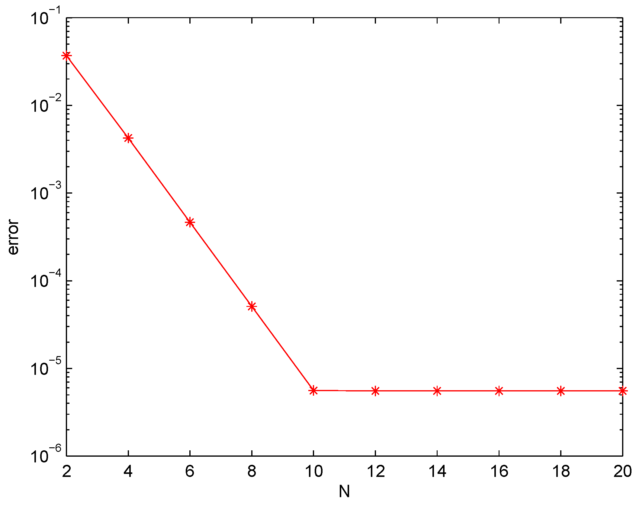
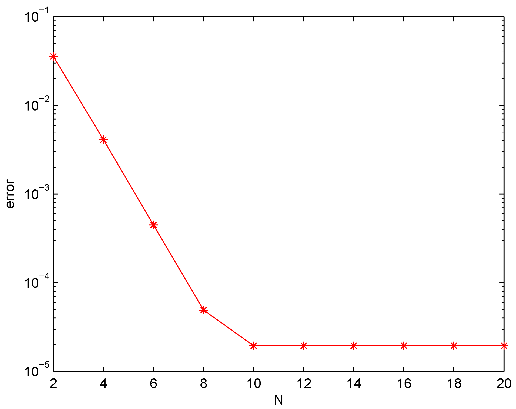
Finally, choosing $M=1000$ and $J=100$, we verified the convergence rate in the spatial direction with respect to the polynomial degree N. Figure 1 and Figure 2 plot the maximum errors in the $L^2$-norm for different $\sigma$ and $\beta$ in the semi-log scale by taking $r=(2-\beta )/\sigma$. It shows that the errors exponentially decay, namely the spectral accuracy in the spatial direction was obtained.

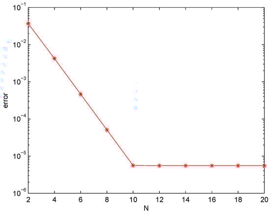
Figure 1. Spatial convergence orders for $\sigma =\beta =0.5$.

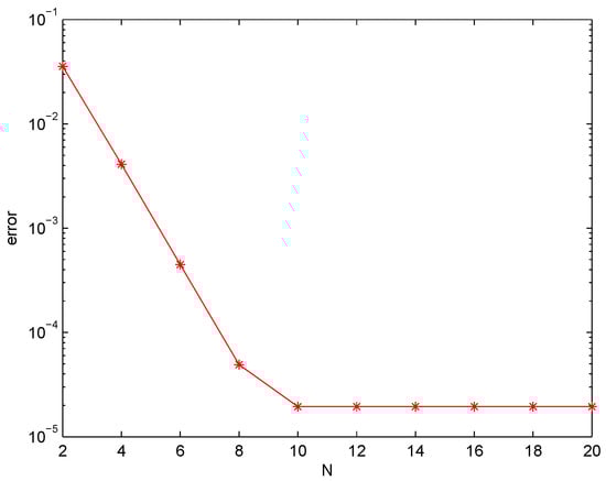
Figure 2. Spatial convergence orders for $\sigma =0.4,\beta =0.6$.

7. Conclusions

The nonlinear distributed-order time-fractional diffusion equations with a weak singularity on an unbounded domain have been numerically solved. An $\alpha$-robust fully discrete scheme has been developed based on the L1 formula on a graded mesh in time and the Galerkin spectral method using the Laguerre function in space. We established an $\alpha$-robust discrete Gronwall inequality and the a priori error estimation of the numerical solution. Then, we obtained that the numerical solution exists and is unique. Next, we proved that the scheme is $\alpha$-robust stable and convergent using the proposed Gronwall inequality, where the convergence rate was $O(M^{-min\{r\sigma ,2-\beta +\frac{\Delta \alpha }{2}\}}+N^{\frac{1-s}{2}}+\Delta {\alpha }^2)$. It should be pointed out that the error estimation was obtained based on the realistic regularity conditions of the solution. The numerical results have demonstrated the sharpness of the error estimation.

References

- Scher, H.; Montroll, E. Anomalous transit-time dispersion in amorphous solids. Phys. Rev. B 1975, 12, 2455. [Google Scholar] [CrossRef]
- Caputo, M.; Mainardi, F. Linear models of dissipation in anelastic solids. Riv. Nuovo C. 1971, 1, 161–198. [Google Scholar] [CrossRef]
- Koeller, R.C. Applications of fractional calculus to the theory of viscoelasticity. J. Appl. Mech. 1984, 51, 299–307. [Google Scholar] [CrossRef]
- Lubich, C. Discretized fractional calculus. SIAM J. Math. Anal. 1986, 17, 704–719. [Google Scholar] [CrossRef]
- Sun, Z.Z.; Wu, X.N. A fully discrete difference scheme for a diffusion-wave system. Appl. Numer. Math. 2006, 56, 193–209. [Google Scholar] [CrossRef]
- Lin, Y.M.; Xu, C.J. Finite difference/spectral approximations for the time-fractional diffusion equation. J. Comput. Phys. 2007, 225, 1533–1552. [Google Scholar] [CrossRef]
- Alikhanov, A.A. A new difference scheme for the time fractional diffusion equation. J. Comput. Phys. 2015, 280, 424–438. [Google Scholar] [CrossRef]
- Stynes, M.; O’riordan, E.; Gracia, J.L. Error analysis of a finite difference method on graded meshes for a time-fractional diffusion equation. SIAM J. Numer. Anal. 2017, 55, 1057–1079. [Google Scholar] [CrossRef]
- Jin, B.T.; Lazarov, R.; Zhou, Z. Two fully discrete schemes for fractional diffusion and diffusion-wave equations with nonsmooth data. SIAM J. Sci. Comput. 2016, 38, A146–A170. [Google Scholar] [CrossRef]
- Cao, W.R.; Zeng, F.H.; Zhang, Z.Q.; Karniadakis, G.E. Implicit-explicit difference schemes for nonlinear fractional differential equations with nonsmooth solutions. SIAM J. Sci. Comput. 2016, 38, A3070–A3093. [Google Scholar] [CrossRef]
- Sinai, Y.G. The limiting behavior of a one-dimensional random walk in a random medium. Theory Probab. Appl. 1982, 27, 256–268. [Google Scholar] [CrossRef]
- Chechkin, A.V.; Gorenflo, R.; Sokolov, I.M. Retarding subdiffusion and accelerating superdiffusion governed by distributed order fractional diffusion equations. Phys. Rev. E 2002, 66, 046129. [Google Scholar] [CrossRef] [PubMed]
- Chechkin, A.V.; Klafter, J.; Sokolov, I.M. Fractional Fokker-Planck equation for ultraslow kinetics. Europhys. Lett. 2003, 63, 326–332. [Google Scholar] [CrossRef]
- Hu, X.; Liu, F.; Anh, V.; Turner, I. A numerical investigation of the time distributed-order diffusion model. ANZIAM J. 2014, 55, C464–C478. [Google Scholar] [CrossRef]
- Chen, H.; Lü, S.J.; Chen, W.P. Finite difference/spectral approximations for the distributed order time fractional reaction-diffusion equation on an un bounded domain. J. Comput. Phys. 2016, 315, 84–97. [Google Scholar] [CrossRef]
- Gao, G.H.; Sun, Z.Z. Two alternating direction implicit difference schemes with the extrapolation method for the two-dimensional distributed-order differential equations. Comput. Math. Appl. 2015, 69, 926–948. [Google Scholar] [CrossRef]
- Gao, G.H.; Sun, Z.Z. Two alternating direction implicit difference schemes for two-dimensional distributed-order fractional diffusion equations. J. Sci. Comput. 2016, 66, 1281–1312. [Google Scholar] [CrossRef]
- Sakamoto, K.; Yamamoto, M. Initial value/boundary value problems for fractional diffusion-wave equations and applications to some inverse problems. J. Math. Anal. Appl. 2011, 382, 426–447. [Google Scholar] [CrossRef]
- Ren, J.C.; Chen, H. A numerical method for distributed order time fractional diffusion equation with weak singular solutions. Appl. Math. Lett. 2019, 96, 159–165. [Google Scholar] [CrossRef]
- Shen, J.; Tang, T.; Wang, L.L. Spectral Methods: Algorithm and Application; Springer-Verlag: Berlin/Heidelberg, Gemany, 2011. [Google Scholar]
- Dahlquist, G.Å. Björck, Numerical Methods in Scientific Computing; Society for Industrial and Applied Mathematics: Philadelphia, PA, USA, 2008; Volume 1. [Google Scholar]
- Chen, H.; Hu, X.H.; Ren, J.C.; Sun, T.; Tang, Y.F. L1 scheme on graded mesh for the linearized time fractional KdV equation with initial singularity. Int. J. Mod. Sim. Sci. Comp. 2019, 10, 1941006. [Google Scholar] [CrossRef]
- Temam, R. Navier-Stokes Equations: Theory and Numerical Analysis, Studies in Mathematics and Its Applications 2; North-Holland Publishing: Amsterdam, The Netherlands, 1977. [Google Scholar]
- Chen, H.; Stynes, M. Blow-up of error estimates in time-fractional initial-boundary value problems. IMA J. Numer. Anal. 2021, 41, 974–997. [Google Scholar] [CrossRef]
- Huang, C.B.; Stynes, M.; Chen, H. An α-robust finite element method for a multi-term time-fractional diffusion problem. J. Comput. Appl. Math. 2021, 389, 113334. [Google Scholar] [CrossRef]
- Huang, C.B.; Stynes, M. α-robust error analysis of a mixed finite element method for a time-fractional biharmonic equation Numer. Algorithm 2021, 87, 1749–1766. [Google Scholar] [CrossRef]
Disclaimer/Publisher’s Note: The statements, opinions and data contained in all publications are solely those of the individual author(s) and contributor(s) and not of MDPI and/or the editor(s). MDPI and/or the editor(s) disclaim responsibility for any injury to people or property resulting from any ideas, methods, instructions or products referred to in the content. |
© 2024 by the authors. Licensee MDPI, Basel, Switzerland. This article is an open access article distributed under the terms and conditions of the Creative Commons Attribution (CC BY) license (https://creativecommons.org/licenses/by/4.0/).