Quasi-P-Wave Reverse Time Migration in TTI Media with a Generalized Fractional Convolution Stencil

Abstract

In seismic modeling and reverse time migration (RTM), incorporating anisotropy is crucial for accurate wavefield modeling and high-quality images. Due to the trade-off between computational cost and simulation accuracy, the pure quasi-P-wave equation has good accuracy to describe wave propagation in tilted transverse isotropic (TTI) media. However, it involves a fractional pseudo-differential operator that depends on the anisotropy parameters, making it unsuitable for resolution using conventional solvers for fractional operators. To address this issue, we propose a novel pure quasi-P-wave equation with a generalized fractional convolution operator in TTI media. First, we decompose the conventional pure quasi-P-wave equation into an elliptical anisotropy equation and a fractional pseudo-differential correction term. Then, we use a generalized fractional convolution stencil to approximate the spatial-domain pseudo-differential term through the solution of an inverse problem. The proposed approximation method is accurate, and the wavefield modeling method based on it also accurately describes quasi-P-wave propagation in TTI media. Moreover, it only increases the computational cost for calculating mixed partial derivatives compared to those in vertical transverse isotropic (VTI) media. Finally, the proposed wavefield modeling method is utilized in RTM to correct the anisotropic effects in seismic imaging. Numerical RTM experiments demonstrate the flexibility and viability of the proposed method.

1. Introduction

Reverse time migration (RTM) is an accurate seismic imaging method used to image complex structures in the subsurface [1,2,3]. It is suitable for lateral velocity variation and is not constrained by steeply dipping limitations. Over time, RTM has been expanded from acoustic isotropic media to viscoelastic anisotropic media [4,5,6] and, from adjoint-based migration to least-squares migration [7,8]. In exploration regions with significant anisotropy, such as subsalt sediments and shale reservoirs, neglecting the anisotropy not only results in blurring and mispositioning of events, but also degrades and distorts seismic images [9]. In exploration seismology, the transverse isotropy (TI) model proposed by [10] is widely used. The symmetry axes in the TI model can be either vertical or tilted, which are known as vertical transverse isotropy (VTI) or tilted transverse isotropy (TTI) media, respectively. Various wave equations have been developed in previous studies to describe the propagation of seismic waves in TI media.

The elastic wave equation can be used for accurate seismic wave modeling in TI media. In RTM, it is essential to extract pure P- and S-waves from the elastic wavefields for generating images with a clear physical meaning. One direct method is to solve the elastic wave equation and then decompose the elastic wavefields into P- and S-waves using the Helmholtz decomposition [11,12]. However, the cost of wavefield extrapolation using the elastic wave equation is significantly higher than that of the acoustic wave equation [13,14]. Alternatively, simplifying the anisotropic elastic wave equation to a quasi-P-wave equation is more efficient and practical.

According to the P-wave dispersion relation, Ref. [15] proposed a quasi-P-wave equation for transversely isotropic (TI) media by setting the S-wave velocity along the symmetry axis to zero. However, this quasi-P-wave equation suffered from S-wave artifacts and a high computational cost for solving the fourth-order partial derivatives. Later, based on the acoustic approximation of [15], various types of coupled second-order wave equations were developed [4,16,17,18]. These equations are computationally efficient and numerically stable. However, they still produce S-wave artifacts that can affect the quality of the resulting images.

On the other hand, Ref. [19] proposed a pure quasi-P-wave equation that could fundamentally avoid S-wave artifacts. However, this pure quasi-P-wave equation involved a space-fractional pseudo-differential operator that depended on the anisotropy parameters, making it unsuitable for direct resolution using conventional solvers such as the finite-difference method and the pseudo-spectral method [20,21,22]. In order to solve the pure quasi-P-wave equation efficiently, Refs. [23,24] separated the pseudo-differential operator into two terms: a partial differential term and an additional scalar term containing anisotropy parameters. The resulting wave equation could be solved using finite-difference methods and pseudo-spectral methods. Ref. [25] utilized the Taylor expansion to approximate the fractional pseudo-differential operator and solved it using a pseudo-spectral approach, which involved a variable Poisson’s equation associated with anisotropic parameters. Later, Ref. [26] used a new expansion approach based on least-square optimization to approximate the pseudo-differential operator. This method improved the accuracy of the approximation, but there were too many terms to solve in TTI media. The fractional pseudo-differential operator can also be computed in a hybrid space-wavenumber domain using approximation methods [27,28,29,30,31].

In addition to approximating the fractional pseudo-differential operator in the wavenumber domain, it is also very meaningful to obtain the pseudo-differential operator in the spatial domain, i.e., fractional convolution stencils. Once fractional convolution stencils are obtained, they can be used to address partial differential equations. However, solving the pseudo-differential operator in the spatial domain poses significant challenges due to their inherent complexity, and analytical solutions are often elusive [32]. As a result, researchers often resort to numerical methods and computational techniques to investigate the dynamics of systems governed by complex fractional differential equations [33]. Ref. [34] derived exact solutions and dynamic properties of a nonlinear fourth-order time-fractional partial differential equation. Recently, Ref. [35] derived the fractional convolution stencils for space-fractional pseudo-differential operators by solving an optimization problem in the wavenumber domain.

Conventional quasi-P-wave equations in TTI media are often affected by the presence of residual S-waves or require complicated and costly computational strategies. To tackle this challenge, we propose a novel pure quasi-P-wave equation in TTI media. We first decompose the quasi-P-wave equation into an elliptical anisotropy equation and a fractional pseudo-differential correction term. Then, we approximate the fractional pseudo-differential term using a fractional convolution stencil, which is determined by solving a nonlinear inverse problem. Next, in non-elliptically anisotropic regions, these convolution stencils are applied locally to rectify non-elliptically anisotropic effects. In contrast to the coupled quasi-P-wave equations and other approximated pure quasi-P-wave equations, the proposed wave equation does not produce S-wave artifacts and can be efficiently solved using the finite-difference method and local convolution, which can be readily computed in parallel.

The rest of this paper is organized as follows: Firstly, we present the novel pure TTI quasi-P-wave equation with a fractional pseudo-differential correction term. Then, we show the method for approximating the pseudo-differential operator using a generalized fractional convolution stencil. Next, the precision of the proposed approximation method is demonstrated through phase-velocity analyses. Finally, numerical experiments demonstrate the flexibility and viability of the proposed method.

2. Methodology

2.1. Pure Quasi-P-Wave Equation in TTI Media

The 2D quasi-P-wave equation in TTI media [18,35] can be written as

$$\left(\genfrac{}{}{0pt}{}{{\partial }_t^2{\sigma }_{xx}}{{\partial }_t^2{\sigma }_{zz}}\right)={\nu }_0^2\left[\begin{array}{cc}1+2\epsilon & \sqrt{1+2\delta }\\ \sqrt{1+2\delta }& 1\end{array}\right]\left(\genfrac{}{}{0pt}{}{{\partial }_{\widehat{x}}^2{\sigma }_{xx}}{{\partial }_{\widehat{z}}^2{\sigma }_{zz}}\right),$$

(1)

with

$$\begin{array}{c}\hfill {\partial }_{\widehat{x}}^2={(\cos \theta {\partial }_x-\sin \theta {\partial }_z)}^2,\\ \hfill {\partial }_{\widehat{z}}^2={(\sin \theta {\partial }_x+\cos \theta {\partial }_z)}^2,\end{array}$$

(2)

where $\epsilon$ and $\delta$ are Thomsen’s anisotropic parameters [10]; $\theta$ denotes the tilt angle of the symmetry axis; ${\sigma }_{xx}$ and ${\sigma }_{zz}$ are the normal stresses along the x and z directions; ${\nu }_0$ is the P-wave velocity along the symmetry axis; and ${\partial }_{\widehat{x}}^2$ and ${\partial }_{\widehat{z}}^2$ are second-order spatial derivatives, evaluated in a rotated coordinate system that is aligned with the axis of symmetry. This coupled quasi-P-wave equation can be solved by using conventional finite-difference methods, but it generates S-wave artifacts and is unstable for $\epsilon <\delta$ [4,16]. By transforming the TTI quasi-P-wave equation into the frequency-wavenumber domain by using the Fourier pairs ${\left(-{\nabla }^2\right)}^{\frac{ϵ}{2}}=k^{ϵ}$ and $\frac{\partial }{\partial t}=i\omega$, we can obtain the Christoffel equation [36] as

$$\left(\genfrac{}{}{0pt}{}{{\omega }^2\widetilde{{\sigma }_{xx}}}{{\omega }^2\widetilde{{\sigma }_{zz}}}\right)={\nu }_0^2\left[\begin{array}{cc}{\left(k_x\cos \theta -k_z\sin \theta \right)}^2(1+2\epsilon )& {\left(k_x\sin \theta +k_z\cos \theta \right)}^2\sqrt{1+2\delta }\\ {\left(k_x\cos \theta -k_z\sin \theta \right)}^2\sqrt{1+2\delta }& {\left(k_x\sin \theta +k_z\cos \theta \right)}^2\end{array}\right]\left(\genfrac{}{}{0pt}{}{\widetilde{{\sigma }_{xx}}}{\widetilde{{\sigma }_{zz}}}\right),$$

(3)

where $\omega$ is the angular frequency, $\tilde{\sigma }$ is the stress tensor in the wavenumber domain, and $k_x$ and $k_z$ are the horizontal and vertical wavenumbers.

The pure quasi-P-wave equation can be factorized from Equation (3) as

$$\left\{{\omega }^2-\frac{1}{2}{v}^2\left[{\widehat{k_x}}^2\left(1+2\epsilon \right)+{\widehat{k_z}}^2+\sqrt{{({\widehat{k_x}}^2\left(1+2\epsilon \right)+{\widehat{k_z}}^2)}^2-8{\widehat{k_x}}^2{\widehat{k_z}}^2(\epsilon -\delta )}\right]\right\}\widetilde{{\sigma }_{zz}}=0.$$

(4)

with

$$\begin{array}{c}\hfill \widehat{k_x}=k_x\cos \theta -k_z\sin \theta ,\\ \hfill \widehat{k_z}=k_x\sin \theta +k_z\cos \theta ,\end{array}$$

(5)

where $\omega$ is the angular frequency, ${\tilde{\sigma }}_{zz}$ is the stress along z directions in the wavenumber domain, and $\widehat{k_x}$ and $\widehat{k_z}$ are the horizontal and vertical wavenumbers in the rotated coordinate system. This equation accurately describes the kinematics of acoustic wavefields in the TTI media and is free from residual S-waves and the instability issue for $\epsilon <\delta$. However, it involves a pseudo-differential term that depends on the anisotropy parameters. Conventional fractional pseudo-differential operators can be solved by using hybrid-domain methods. In these methods, the stress $\sigma$ is transformed from the spatial domain to the wavenumber domain, multiplied by pseudo-differential operators, e.g., $\frac{1}{k_x^2{k}_z^2}$, and then transformed back to the spatial domain. However, the anisotropy parameters are spatial, so the pseudo-differential term in Equation (3) cannot directly multiply the stress ${\tilde{\sigma }}_{zz}$, and Equation (3) cannot be directly solved by using conventional solvers. Many approximation methods and complicated hybrid-domain methods [23,26] have been proposed to address this issue, but they all suffer from low approximation accuracy or high computation cost.

To address this issue, we first rewrite the pseudo-differential term of the pure quasi-P-wave Equation (3) as

$$\sqrt{{\left[{\widehat{k_x}}^2\left(1+2\epsilon \right)+{\widehat{k_z}}^2\right]}^2-8{\widehat{k_x}}^2{\widehat{k_z}}^2(\epsilon -\sigma )}=\left[{\widehat{k_x}}^2\left(1+2\epsilon \right)+{\widehat{k_z}}^2\right]\sqrt{1-\frac{8{\widehat{k_x}}^2{\widehat{k_z}}^2(\epsilon -\delta )}{{\left[{\widehat{k_x}}^2\left(1+2\epsilon \right)+{\widehat{k_z}}^2\right]}^2}},$$

(6)

where ${\widehat{k_x}}^2\left(1+2\epsilon \right)+{\widehat{k_z}}^2$ is an elliptically anisotropic term, which can be directly solved using conventional solvers, and $\sqrt{1-\frac{8{\widehat{k_x}}^2{\widehat{k_z}}^2(\epsilon -\delta )}{{\left[{\widehat{k_x}}^2\left(1+2\epsilon \right)+{\widehat{k_z}}^2\right]}^2}}$ is a fractional pseudo-differential correction term that requires an efficient approximation method for its solution. The magnitude of this fractional pseudo-differential term is much smaller than that of the entire square root term in Equation (4), so it has a better tolerance for approximation error compared with the entire square root term.

Then, we derive the novel pure quasi-P-wave equation by inserting Equation (6) into Equation (4) and present it in the coordinate system without rotation as

$$\left\{{\omega }^2-\frac{1}{2}{v}^2\left[{\left(k_x\cos \theta -k_z\sin \theta \right)}^2\left(1+2\epsilon \right)+{(k_x\sin \theta +k_z\cos \theta )}^2\right](1+\tilde{\Lambda }(k_x,k_z,\epsilon ,\delta ,\theta ))\right\}\widehat{p}=0,$$

(7)

with

$$\tilde{\Lambda }(k_x,k_z,\epsilon ,\delta ,\theta )=\sqrt{1-\frac{8{\left(k_x\cos \theta -k_z\sin \theta \right)}^2(k_x\sin \theta +k_z{\cos \theta )}^2\left(\epsilon -\delta \right)}{{\left[{\left(k_x\cos \theta -k_z\sin \theta \right)}^2\left(1+2\epsilon \right)+{(k_x\sin \theta +k_z\cos \theta )}^2\right]}^2}}.$$

(8)

Next, by using the Fourier pairs ${\left(-{\nabla }^2\right)}^{\frac{ϵ}{2}}=k^{ϵ}$ and $\frac{\partial }{\partial t}=i\omega$, we collect the terms of the pure quasi-P-wave Equation (7) and transform it from the frequency-wavenumber domain to the time-space domain as

$$\frac{{\partial }^{2}p}{\partial t^2}=\frac{1}{2}{v}^2\left[\left(1+2\epsilon cos{\theta }^2\right)\frac{{\partial }^2}{\partial x^2}+2\epsilon sin{\theta }^2\frac{{\partial }^2}{\partial z^2}-4\epsilon sin\theta cos\theta \frac{{\partial }^2}{\partial x\partial z}\right](p+\Lambda \left(x,z,\epsilon ,\delta ,\theta \right)\ast p),$$

(9)

with

$$\Lambda \left(x,z,\epsilon ,\delta ,\theta \right)=\frac{1}{2\pi }{\displaystyle {\int \int }_{-\infty }^{+\infty }}\tilde{\Lambda }\left(k_x,k_z,\epsilon ,\delta ,\theta \right)e^{i{k}_{x}x}{e}^{i{k}_{z}z}d{k}_{x}d{k}_z,$$

(10)

where ∗ denotes the convolution, and $\Lambda \left(x,z,\epsilon ,\delta ,\theta \right)$ is a fractional pseudo-differential correction operator in the space domain. The novel pure quasi-P-wave Equation (9) can be solved directly using conventional finite-difference methods and local convolutions, as long as the spatial-domain fractional pseudo-differential correction operator $\Lambda \left(x,z,\epsilon ,\delta ,\theta \right)$ is obtained.

2.2. Approximating the Pseudo-Differential Operator Using a Generalized Fractional Convolution Stencil

The fractional pseudo-differential operator in the space domain $\Lambda \left(x,z,\epsilon ,\delta ,\theta \right)$ is dependent on the anisotropic parameters $\epsilon$, $\delta$ and $\theta$. Here, we describe how to approximate an operator $\Lambda \left(x,z\right)$ for a set of $\epsilon$, $\delta$ and $\theta$ using a generalized fractional convolution stencil. The operator $\Lambda \left(x,z\right)$ is transformed from the space domain to the wavenumber domain using the 2D Fourier transform as

$$\tilde{\Lambda }\left(k_x,k_z\right)={\int \int }_{-\infty }^{+\infty }\Lambda \left(x,z\right)e^{-i{k}_{x}x}{e}^{-i{k}_{z}z}dxdz.$$

(11)

Then, we use the Euler formula to simplify the exponential function as

$$\begin{array}{c}\hfill \tilde{\Lambda }\left(k_x,k_z\right)={\int \int }_{-\infty }^{+\infty }\Lambda \left(x,z\right)\left(cos{k}_{x}xcosx{k}_{z}z+isin{k}_{x}xcosx{k}_{z}z\right.\\ \hfill \left.+isin{k}_{z}zcosx{k}_{x}x-sin{k}_{z}zsinx{k}_{x}x\right)dxdz.\end{array}$$

(12)

Due to the operator’s even symmetry, i.e., $\Lambda \left(x,z\right)=\Lambda \left(-x,-z\right)$, the second and third trigonometric terms in Equation (12) do not contribute to the integration. Thus, Equation (12) is simplified to

$$\tilde{\Lambda }\left(k_x,k_z\right)={\int \int }_{-\infty }^{+\infty }\Lambda \left(x,z\right)cos\left(k_{x}x+k_{z}z\right)dxdz.$$

(13)

We use a generalized fractional convolution stencil to discretize $\Lambda \left(x,z\right)$ and $\tilde{\Lambda }\left(k_x,k_z\right)$ can be approximated as

$$\tilde{\Lambda }\left(k_x,k_z\right)\approx \sum _{i=-a}^a\sum _{i=-a}^a\Lambda \left(i\Delta x,j\Delta z\right)cos\left(k_{x}i\Delta x+k_{z}j\Delta z\right),$$

(14)

where a is the half-length of the generalized fractional convolution stencil, which was set to 5 in this study, and $\Delta x$ and $\Delta z$ denote the grid increments along the x and z directions.

Next, by constraining the wavenumber within the range of $\left[-\frac{9}{10}\pi ,\frac{9}{10}\pi \right]$, we calculate the generalized fractional convolution stencil by minimizing the difference between the true and approximated pseudo-differential operators. The misfit function for this inverse problem can be expressed as

$$F\left(\Lambda \left(i\Delta x,j\Delta z\right)\right)={∥{\tilde{\Lambda }}_{true}\left(k_x,k_z\right)-\sum _{i=-a}^a\sum _{i=-a}^a\Lambda \left(i\Delta x,j\Delta z\right)cos\left(k_{x}i\Delta x+k_{z}j\Delta z\right)∥}^2,$$

(15)

where ${\tilde{\Lambda }}_{true}$ represents the true fractional pseudo-differential operator in the wavenumber domain (8). We used the interior-reflective Newton algorithm [37] to solve this least-squares inverse problem. This algorithm is quadratically and globally convergent, and the identification of an “activity set” is not necessary for it.

We present a calculated generalized fractional convolution stencil for a case with $\epsilon =0.2$, $\delta =0.1$ and $\theta ={30}^{\circ }$ and compare the corresponding true and approximated pseudo-differential operators in Figure 1. As shown in Figure 1, the coefficient of the central point in the fractional convolution stencil is dominant, and the relative error is only about $2.0535\times {10}^{-9}$. This indicates that the proposed approximation method can accurately generate a fractional convolution stencil to approximate the spatial-domain fractional pseudo-differential operator.

To further evaluate the accuracy of the approximation, we compared the phase velocities calculated using the true and approximated fractional pseudo-differential operator $\tilde{\Lambda }$, which is given by

$$c\left(k_x,k_z\right)=\frac{\sqrt{\frac{1}{2}{v}^2\left[{\left(k_x\cos \theta -k_z\sin \theta \right)}^2\left(1+2\epsilon \right)+{\left(k_x\sin \theta +k_z\cos \theta \right)}^2\right](1+\tilde{\Lambda })}}{\sqrt{k_x^2+k_z^2}},$$

(16)

The resulting phase velocities for v = 3000 m/s, $\epsilon =0.2$, $\delta =0.1$ and $\theta ={30}^{\circ }$ are shown in Figure 2. The relative error of $0.1\%$ indicates that the proposed approximation method has good accuracy.

2.3. Numerical Implementation in Modeling and RTM

Before conducting pure quasi-P-wave wavefield modeling, we need to prepare a fractional convolution stencil library. In this study, we set the range $0\le \epsilon \le 0.5$, $-0.5\le \epsilon -\delta \le 0.5$ with a 0.01 increment, and $-{90}^{\circ }\le \theta \le {90}^{\circ }$ with a $1^{\circ }$ increment. In total, 932,331 fractional convolution stencils with a size of 11 × 11 were calculated using the proposed approximation method. The convolution stencils were organized into a fractional convolution stencil library, which could be repeatedly applied to wavefield extrapolation. The numerical implementation of pure quasi-P-wave modeling for a TTI model can be summarized as follows:

• In regions with non-elliptical anisotropy, load the convolution stencils from the fractional convolution stencil library based on the anisotropic parameters.
• Convolve the convolution stencil with the stress field as $\Lambda (x,z,\epsilon ,\delta ,\theta )\ast p$ to correct the non-elliptically anisotropic effects.
• Use the central finite-difference scheme to calculate $\frac{{\partial }^2}{\partial x^2}$, $\frac{{\partial }^2}{\partial z^2}$ and $\frac{{\partial }^2}{\partial x\partial z}$ of the corrected stress field $p+\Lambda (x,z,\epsilon ,\delta ,\theta )\ast p$.
• Update the wavefield using the second-order equation finite in time $p^{n+1}=2p^n-p^{n-1}+\frac{1}{2}\Delta t^2{v}^2\left[(1+2\epsilon cos{\theta }^2)\frac{{\partial }^2}{\partial x^2}+2\epsilon sin{\theta }^2\frac{{\partial }^2}{\partial z^2}-4\epsilon sin\theta cos\theta \frac{{\partial }^2}{\partial x\partial z}\right]\left(p+\Lambda (x,z,\epsilon ,\delta ,\theta )\ast p\right)$.

After solving the pure quasi-P-wave equation for the stress wavefields of the source and receiver, the RTM image can be calculated by using the zero-lag cross-correlation imaging condition as

$$I\left(\mathbf{x}\right)=\frac{{\int }_0^T{p}_s\left(\mathbf{x}\right)p_r\left(\mathbf{x}\right)dt}{{\int }_0^T{p}_s\left(\mathbf{x}\right)p_s\left(\mathbf{x}\right)dt},$$

(17)

where $\mathbf{x}$ represents the spatial coordinates for underground imaging, $p_s\left(\mathbf{x}\right)$ and $p_r\left(\mathbf{x}\right)$ are the source wavefield and receiver wavefield, and $dt$ and T are the time step and recording duration, respectively.

3. Numerical Examples

In this section, four numerical examples are used to illustrate the performance of the proposed pure quasi-P-wave modeling and RTM in TTI media. For comparisons purposes, we also calculated the wavefields and RTM images in both isotropic and VTI media. In all numerical experiments, we calculated $\frac{{\partial }^2}{\partial x^2}$ and $\frac{{\partial }^2}{\partial z^2}$ by using the second-order central finite-difference scheme with 20th-order accuracy and calculated $\frac{{\partial }^2}{\partial x\partial z}$ by using the first-order central finite-difference scheme with 20th-order accuracy.

3.1. Homogeneous Model

In the first example, we tested the proposed modeling approach for a homogeneous TTI model ($v_P$ = 3 km/s, $\epsilon$ = 0.2, $\delta$ = 0.1 and $\theta ={30}^{\circ }$). A total of 501 × 501 grid points were used in the simulations with a spatial increment of 10 m. An explosive source was placed in the center of the model. The source’s time function was a 10-Hz Ricker wavelet, and the time step was 0.001 s. For comparisons, we also computed the VTI wavefields by solving the wave equation [4]. Figure 3 shows wavefield snapshots of isotropic, VTI and TTI modeling at 0.6 s. The method of [4] suffers from S-wave artifacts (Figure 3b). By contrast, there are no S-wave artifacts in wavefields simulated by the proposed method due to the use of the pure quasi-P-wave equation (Figure 3c). As shown in Figure 3, the TTI wavefield is rotated based on the tilted angles of the symmetry axes, in contrast to the VTI wavefield.

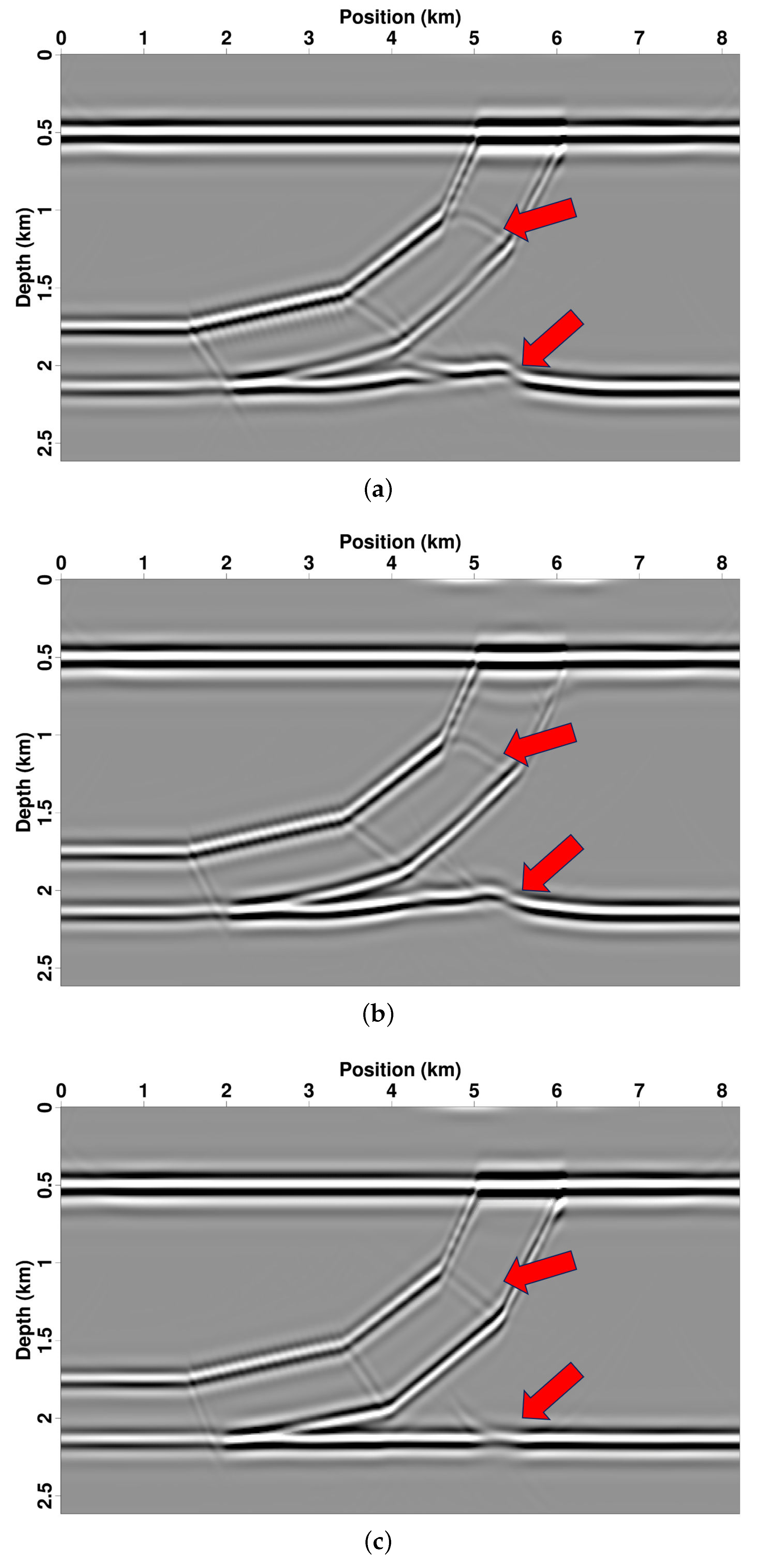
3.2. Overthrust TTI Model

Then, we used an overthrust TTI model (Figure 4) to test the feasibility of the proposed method. In total, 822 × 262 grid points were used, with a spatial increment of 10 m. The true model was smoothed using a triangular filter with dimensions of 50 m × 50 m to construct the migration velocity and anisotropic parameter models. A total of 301 explosive sources were evenly distributed on the surface, with a 30 m spacing. These sources were recorded by 500 receivers covering a 5 km aperture. The recording duration was 3 s, with a time sample increment of 1 ms. The synthetic shot gathers are shown in Figure 5. We present the migration images obtained using isotropic, VTI and TTI RTM in Figure 6. The reflectors in the region with a steep tilt angle appear distorted and misplaced, as indicated by the upper red arrows in Figure 6a,b. Moreover, for the reflectors in the isotropic region, distorted and misplaced features also appear, as indicated by the other red arrows in Figure 6a,b. Conversely, the proposed TTI RTM method produces clear images with accurate kinematic information and focused events (Figure 6c).

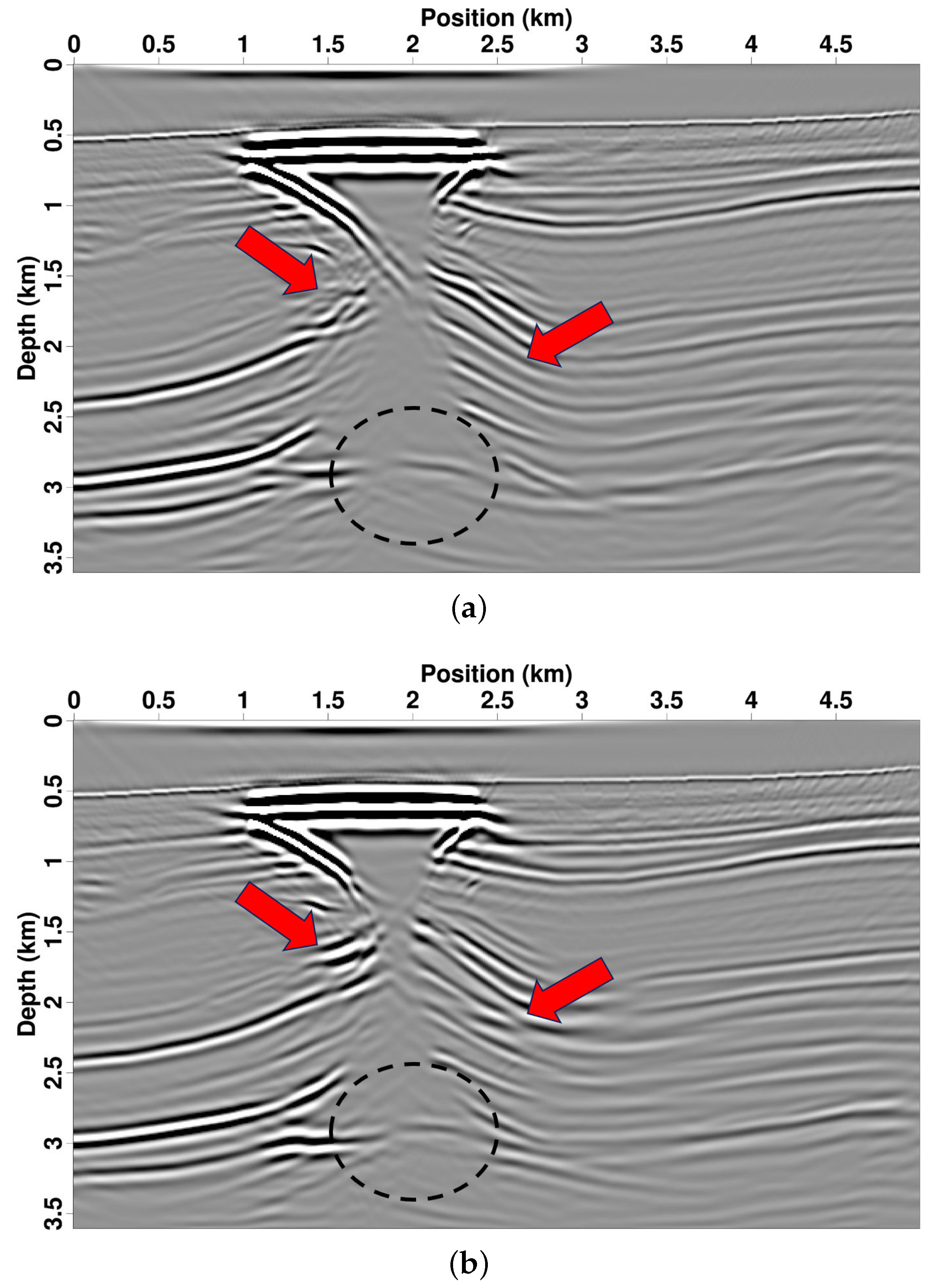
3.3. 2007 BP TTI Model

To further verify the feasibility and effectiveness of the proposed method, we conducted RTM experiments using the proposed TI RTM methods on a modified 2007 BP TTI model (Figure 7). As shown in Figure 7, an intrusive rock mass with isotropic properties is depicted, and the variations in dip angle near this rock mass are very pronounced, posing a significant challenge for underground imaging. The 2007 BP TTI model was discretized with a grid of 500 × 361, with a spatial increment of 10 m. In total, 166 explosive sources with a 25 Hz Ricker wavelet were evenly distributed on the surface, with a spacing of 30 m. In addition, 400 receivers were evenly distributed on the surface. The recording duration was 4 s, with a time sample interval of 0.5 ms. Shot gathers are shown in Figure 8. The migration images acquired through isotropic, VTI and TTI RTM are presented in Figure 9. The reflectors near the intrusive rock mass in the isotropic and VTI images are severely distorted and misplaced due to the steep dip angles, as indicated by the red arrows in Figure 9a,b. Moreover, neglecting the anisotropy also degrades and distorts images in the root regions of the intrusive rock mass (circled regions in Figure 9a,b). On the contrary, the proposed TTI RTM can correct the distortion in seismic wave propagation in TTI media, producing clear images with accurate kinematic information and focused events (Figure 9c).

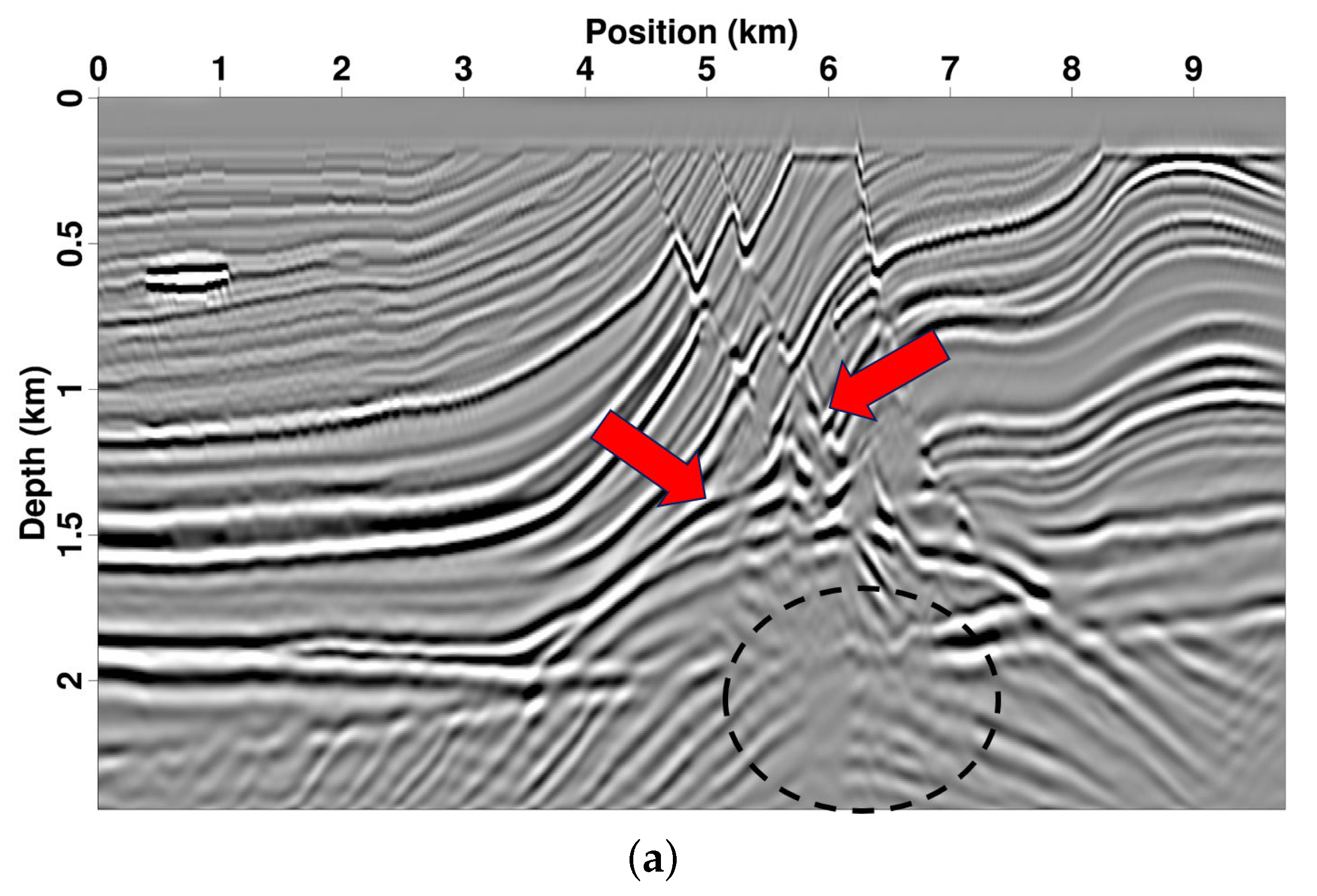
3.4. Marmousi TTI Model

In this experiment, we used the modified Marmousi TTI model to assess the adaptability of the proposed quasi-P-wave imaging method for complex structures. Velocity and anisotropy models are presented in Figure 10. A total of 433 shots were set with a spacing of 22.5 m. Each shot was recorded using 400 receivers spaced 7.5 m apart, covering an aperture of 3 km. The recording duration was 4 s, with a time sample interval of 0.5 ms. The source’s time function was a Ricker wavelet. The peak frequency was 20 Hz. The synthetic shot gathers are shown in Figure 11. Migrated images using isotropic, VTI and TTI RTM are presented in Figure 12. The isotropic and VTI images for the faults and associated faulted blocks appear distorted and misplaced, as shown in Figure 12a,b. Moreover, the reflectors within the anticline exhibit low amplitudes and are contaminated by migration noises. After correcting the effects of anisotropy, the faults and associated faulted blocks are well imaged, and the reflectors within the anticline reservoir become more continuous and easily interpretable (Figure 12c).

4. Discussion

We directly approximated the fractional pseudo-differential term using a fractional convolution stencil, eliminating the need for the Fourier transform required by Poisson’s solvers and hybrid-domain algorithms. Taking a wavefield modeling experiment for a homogeneous model with 501 × 501 grid points as an example, using the least-squares optimization method with the Fourier transform [26] took 487.112963 s, while using the proposed method only took 57.418852 s.

The novel pure quasi-P-wave can be directly solved using conventional finite-difference methods and local spatial convolution. Computational efficiency can be significantly improved through parallel computation with domain decomposition. Our approach approximates the correction term, which accounts for the non-ellipticity of anisotropic wavefields, and thus yields significantly fewer errors than the approximation method proposed by [35].

In comparison with those in VTI media, the proposed approach in TTI media only mainly adds computational cost and memory usage for the calculation of mixed partial derivatives. Furthermore, the development of the proposed method for 3D modeling is straightforward, with the addition of an azimuth of the symmetry axis and a new coordinate axis. A 0.01 increment was used in the calculation of convolution stencils. Smaller increments can be used to increase accuracy, but with larger memory storage. In addition, once the fractional convolution stencil library is precalculated, it can be repeatedly used for modeling and imaging in various models.

5. Conclusions

In this study, we proposed a practical pure quasi-P-wave modeling and RTM approach in the TTI media. We first derived the novel pure TTI quasi-P-wave equation with a fractional pseudo-differential correction term. Then, we approximated the pseudo-differential operators by solving nonlinear inverse problems and created a library of fractional convolution stencils, which comprised 932,331 stencils. Next, the precision and adaptability of the proposed forward modeling approach were demonstrated through phase-velocity analyses and forward modeling experiments. Numerical examples demonstrated that the proposed TTI RTM could correct the anisotropic effects and produce accurate subsurface images for complex structures, such as intrusive rock masses with steep dip angles, anticlines, faults and associated faulted blocks.

References

1. Baysal, E.; Kosloff, D.D.; Sherwood, J.W. Reverse time migration. Geophysics 1983, 48, 1514–1524. [Google Scholar] [CrossRef]
2. McMechan, G.A. Migration by extrapolation of time-dependent boundary values. Geophys. Prospect. 1983, 31, 413–420. [Google Scholar] [CrossRef]
3. Whitmore, N.D. Iterative depth migration by backward time propagation. In SEG Technical Program Expanded Abstracts 1983; Society of Exploration Geophysicists: Houston, TX, USA, 1983; pp. 382–385. [Google Scholar]
4. Zhang, Y.; Zhang, H.; Zhang, G. A stable TTI reverse time migration and its implementation. Geophysics 2011, 76, WA3–WA11. [Google Scholar] [CrossRef]
5. Mu, X.; Huang, J.; Li, Z.; Liu, Y.; Su, L.; Liu, J. Attenuation compensation and anisotropy correction in reverse time migration for attenuating tilted transversely isotropic media. Surv. Geophys. 2022, 43, 737–773. [Google Scholar] [CrossRef]
6. Qiao, Z.; Chen, T.; Sun, C. Anisotropic Attenuation Compensated Reverse Time Migration of Pure qP-Wave in Transversely Isotropic Attenuating Media. Surv. Geophys. 2022, 43, 1435–1467. [Google Scholar] [CrossRef]
7. Nemeth, T.; Wu, C.; Schuster, G.T. Least-squares migration of incomplete reflection data. Geophysics 1999, 64, 208–221. [Google Scholar] [CrossRef]
8. Yang, J.; Huang, J.; Li, Z.; Zhu, H.; McMechan, G.; Zhang, J.; Hu, C.; Zhao, Y. Mitigating velocity errors in least-squares imaging using angle-dependent forward and adjoint Gaussian beam operators. Surv. Geophys. 2021, 42, 1305–1346. [Google Scholar] [CrossRef]
9. Huang, T.; Zhang, Y.; Zhang, H.; Young, J. Subsalt imaging using TTI reverse time migration. Lead. Edge 2009, 28, 448–452. [Google Scholar] [CrossRef]
10. Thomsen, L. Weak elastic anisotropy. Geophysics 1986, 51, 1954–1966. [Google Scholar] [CrossRef]
11. Sripanich, Y.; Fomel, S.; Sun, J.; Cheng, J. Elastic wave-vector decomposition in heterogeneous anisotropic media. Geophys. Prospect. 2017, 65, 1231–1245. [Google Scholar] [CrossRef]
12. Yang, J.; Zhang, H.; Zhao, Y.; Zhu, H. Elastic wavefield separation in anisotropic media based on eigenform analysis and its application in reverse-time migration. Geophys. J. Int. 2019, 217, 1290–1313. [Google Scholar] [CrossRef]
13. Yan, J.; Sava, P. Elastic wave mode separation for tilted transverse isotropy media. Geophys. Prospect. 2012, 60, 29–48. [Google Scholar] [CrossRef]
14. Yong, P.; Huang, J.; Li, Z.; Liao, W.; Qu, L.; Li, Q.; Yuan, M. Elastic-wave reverse-time migration based on decoupled elastic-wave equations and inner-product imaging condition. J. Geophys. Eng. 2016, 13, 953–963. [Google Scholar] [CrossRef]
15. Alkhalifah, T. An acoustic wave equation for anisotropic media. Geophysics 2000, 65, 1239–1250. [Google Scholar] [CrossRef]
16. Zhou, H.; Zhang, G.; Bloor, R. An anisotropic acoustic wave equation for VTI media. In Proceedings of the 68th EAGE Conference and Exhibition incorporating SPE EUROPEC 2006, Vienna, Austria, 12–15 June 2006; EAGE Publications BV: Bunnik, The Netherlands, 2006; p. cp-2. [Google Scholar]
17. Du, X.; Bancroft, J.C.; Lines, L.R. Anisotropic reverse-time migration for tilted TI media. Geophys. Prospect. 2007, 55, 853–869. [Google Scholar] [CrossRef]
18. Duveneck, E.; Milcik, P.; Bakker, P.M.; Perkins, C. Acoustic VTI wave equations and their application for anisotropic reverse-time migration. In SEG Technical Program Expanded Abstracts 2008; Society of Exploration Geophysicists: Houston, TX, USA, 2008; pp. 2186–2190. [Google Scholar]
19. Liu, F.; Morton, S.A.; Jiang, S.; Ni, L.; Leveille, J.P. Decoupled wave equations for P and SV waves in an acoustic VTI media. In Proceedings of the 2009 SEG Annual Meeting, Houston, TX, USA, 25–30 October 2009; OnePetro: Richardson, TX, USA, 2009. [Google Scholar]
20. Xue, Z.; Ma, Y.; Wang, S.; Hu, H.; Li, Q. A Multi-Task Learning Framework of Stable Q-Compensated Reverse Time Migration Based on Fractional Viscoacoustic Wave Equation. Fractal Fract. 2023, 7, 874. [Google Scholar] [CrossRef]
21. Wang, Y.; Lu, J.; Shi, Y.; Wang, N.; Han, L. High-Accuracy Simulation of Rayleigh Waves Using Fractional Viscoelastic Wave Equation. Fractal Fract. 2023, 7, 880. [Google Scholar] [CrossRef]
22. Wang, J.; Yuan, S.; Liu, X. Finite Difference Scheme and Finite Volume Scheme for Fractional Laplacian Operator and Some Applications. Fractal Fract. 2023, 7, 868. [Google Scholar] [CrossRef]
23. Xu, S.; Zhou, H. Accurate simulations of pure quasi-P-waves in complex anisotropic media. Geophysics 2014, 79, T341–T348. [Google Scholar] [CrossRef]
24. Xu, S.; Tang, B.; Mu, J.; Zhou, H. Quasi-P wave propagation with an elliptic differential operator. In SEG Technical Program Expanded Abstracts 2015; Society of Exploration Geophysicists: Houston, TX, USA, 2015; pp. 4380–4384. [Google Scholar]
25. Chu, C.; Macy, B.K.; Anno, P.D. Pure acoustic wave propagation in transversely isotropic media by the pseudospectral method. Geophys. Prospect. 2013, 61, 556–567. [Google Scholar] [CrossRef]
26. Li, X.; Zhu, H. A finite-difference approach for solving pure quasi-P-wave equations in transversely isotropic and orthorhombic media. Geophysics 2018, 83, C161–C172. [Google Scholar] [CrossRef]
27. Fomel, S.; Ying, L.; Song, X. Seismic wave extrapolation using lowrank symbol approximation. Geophys. Prospect. 2013, 61, 526–536. [Google Scholar] [CrossRef]
28. Song, X.; Fomel, S.; Ying, L. Lowrank finite-differences and lowrank Fourier finite-differences for seismic wave extrapolation in the acoustic approximation. Geophys. J. Int. 2013, 193, 960–969. [Google Scholar] [CrossRef]
29. Alkhalifah, T. Effective wavefield extrapolation in anisotropic media: Accounting for resolvable anisotropy. Geophys. Prospect. 2014, 62, 1089–1099. [Google Scholar] [CrossRef]
30. Zhang, Z.d.; Liu, Y.; Alkhalifah, T.; Wu, Z. Efficient anisotropic quasi-P wavefield extrapolation using an isotropic low-rank approximation. Geophys. J. Int. 2018, 213, 48–57. [Google Scholar] [CrossRef]
31. Wu, Z.; Alkhalifah, T.; Zhang, Z. A partial-low-rank method for solving acoustic wave equation. J. Comput. Phys. 2019, 385, 1–12. [Google Scholar] [CrossRef]
32. Wang, R.; Feng, Q.; Ji, J. The discrete convolution for fractional cosine-sine series and its application in convolution equations. AIMS Math. 2024, 9, 2641–2656. [Google Scholar] [CrossRef]
33. Hashemi, M. A variable coefficient third degree generalized Abel equation method for solving stochastic Schrödinger–Hirota model. Chaos Solitons Fractals 2024, 180, 114606. [Google Scholar] [CrossRef]
34. Kai, Y.; Chen, S.; Zhang, K.; Yin, Z. Exact solutions and dynamic properties of a nonlinear fourth-order time-fractional partial differential equation. Waves Random Complex Media 2022, 1–12. [Google Scholar] [CrossRef]
35. Nikonenko, Y.; Charara, M. Explicit finite-difference modeling for the acoustic scalar wave equation in tilted transverse isotropic media with optimal operators. Geophysics 2023, 88, T65–T73. [Google Scholar] [CrossRef]
36. Achenbach, J. Wave Propagation in Elastic Solids; Elsevier: Amsterdam, The Netherlands, 2012. [Google Scholar]
37. Coleman, T.F.; Li, Y. An interior trust region approach for nonlinear minimization subject to bounds. SIAM J. Optim. 1996, 6, 418–445. [Google Scholar] [CrossRef]
Figure 1. Comparison of the true and approximated pseudo-differential operators with the size of 11 × 11 for a case with ε = 0.2, δ = 0.1 and θ = π 6 . (a) The generalized fractional convolution stencil in the space domain, (b) the true fractional pseudo-differential operator in the wavenumber domain, (c) the approximated result in the wavenumber domain and (d) the difference between (c) and (d).
Fractalfract 08 00174 g001
Figure 2. Comparisons of the true and approximated phase velocity for a case with v = 3000 m/s, ε = 0.2 , δ = 0.1 and θ = 30 . (a) The phase velocity calculated using the exact operator, (b) the phase velocity calculated using the approximated operator and (c) the difference between (a) and (b).
Fractalfract 08 00174 g002
Figure 3. Wavefields of isotropic, VTI and TTI modeling at 0.6 s for a case with v = 3000 m/s, ε = 0.2 , δ = 0.1 and θ = 30 . (a) Isotropic wavefield, (b) VTI wavefield simulated using the coupled quasi-P wave equations, (c) VTI wavefield simulated using the proposed approach and (d) TTI wavefield simulated using the proposed approach.
Fractalfract 08 00174 g003
Figure 4. P-wave velocity (a), ε (b), δ (c) and θ (d) for the overthrust TTI model.
Fractalfract 08 00174 g004
Figure 5. Shot gathers simulated by the proposed modeling approach for the overthrust TTI model.
Fractalfract 08 00174 g005
Figure 6. Migration images of the overthrust TTI model using various RTM approaches. (a) Image produced using the isotropic RTM approach, (b) image produced using the proposed VTI RTM approach and (c) image produced using the proposed TTI RTM approach.
Fractalfract 08 00174 g006
Figure 7. P-wave velocity (a), ε (b), δ (c) and θ (d) for the 2007 BP TTI model.
Fractalfract 08 00174 g007
Figure 8. Shot gathers simulated by the proposed modeling approach for the 2007 BP TTI model.
Fractalfract 08 00174 g008
Figure 9. Migration images of the 2007 BP TTI model using various RTM approaches. (a) Image produced using the isotropic RTM approach, (b) image produced using the proposed VTI RTM approach and (c) image produced using the proposed TTI RTM approach.
Fractalfract 08 00174 g009aFractalfract 08 00174 g009b
Figure 10. P-wave velocity (a), ε (b), δ (c) and θ (d) for the Marmousi TTI model.
Fractalfract 08 00174 g010aFractalfract 08 00174 g010b
Figure 11. Shot gathers simulated by the proposed modeling approach for the Marmousi TTI model.
Fractalfract 08 00174 g011
Figure 12. Migration images of the Marmousi TTI model using various RTM approaches. (a) Image obtained using the isotropic RTM approach, (b) image obtained using the proposed VTI RTM approach and (c) image obtained using the proposed TTI RTM approach.
Fractalfract 08 00174 g012aFractalfract 08 00174 g012b
Disclaimer/Publisher’s Note: The statements, opinions and data contained in all publications are solely those of the individual author(s) and contributor(s) and not of MDPI and/or the editor(s). MDPI and/or the editor(s) disclaim responsibility for any injury to people or property resulting from any ideas, methods, instructions or products referred to in the content.