Article

A Novel Technique for Solving the Nonlinear Fractional-Order Smoking Model

by
Abdelhamid Mohammed Djaouti
1,*,
Zareen A. Khan
2,*,
Muhammad Imran Liaqat
3 and
Ashraf Al-Quran
1
1
Department of Mathematics and Statistics, Faculty of Sciences, King Faisal University, Hofuf 31982, Saudi Arabia
2
Department of Mathematical Sciences, College of Science, Princess Nourah bint Abdulrahman University, P.O. Box 84428, Riyadh 11671, Saudi Arabia
3
Abdus Salam School of Mathematical Sciences, Government College University, 68-B, New Muslim Town, Lahore 54600, Pakistan
*
Authors to whom correspondence should be addressed.
Fractal Fract. 2024, 8(5), 286; https://doi.org/10.3390/fractalfract8050286
Submission received: 3 April 2024 / Revised: 3 May 2024 / Accepted: 4 May 2024 / Published: 10 May 2024

Abstract

:
In the study of biological systems, nonlinear models are commonly employed, although exact solutions are often unattainable. Therefore, it is imperative to develop techniques that offer approximate solutions. This study utilizes the Elzaki residual power series method (ERPSM) to analyze the fractional nonlinear smoking model concerning the Caputo derivative. The outcomes of the proposed technique exhibit good agreement with the Laplace decomposition method, demonstrating that our technique is an excellent alternative to various series solution methods. Our approach utilizes the simple limit principle at zero, making it the easiest way to extract series solutions, while variational iteration, Adomian decomposition, and homotopy perturbation methods require integration. Moreover, our technique is also superior to the residual method by eliminating the need for derivatives, as fractional integration and differentiation are particularly challenging in fractional contexts. Significantly, our technique is simpler than other series solution techniques by not relying on Adomian’s and He’s polynomials, thereby offering a more efficient way of solving nonlinear problems.

1. Introduction

Traditional calculus deals with integer-order derivatives and integrals, while fractional calculus (FC) extends these concepts to include derivatives and integrals of non-integer orders, such as fractional and complex orders. FC is particularly useful for modeling systems with memory effects, where the current state depends not only on the immediate past but also on past states over a longer period. This behavior is common in many physical, biological, and engineering systems, where the system retains a memory of its past states or inputs. Memory effects can arise due to various factors, such as delays, relaxation processes, and non-local interactions. FC provides a powerful mathematical framework for modeling systems with memory effects, as it allows for the incorporation of fractional-order derivatives and integrals, enabling more accurate descriptions of complex dynamics. However, in systems exhibiting memory effects, fractional-order derivatives and integrals of non-integer orders are necessary to accurately describe their dynamics. FC allows for the incorporation of memory effects by introducing fractional-order operators, such as the Riemann–Liouville, Caputo, and Grünwald–Letnikov operators. These operators generalize the classical differentiation and integration operators to handle non-integer orders, enabling the modeling of systems with long-term memory and complex dynamics. Systems with memory effects are encountered in various fields, including viscoelastic materials, biological systems, signal processing, and control theory. FC has proven to be particularly valuable in these areas, providing a flexible framework for capturing the intricate behaviors arising from memory effects. By incorporating fractional-order derivatives and integrals, researchers can develop more accurate models and gain a better understanding of the dynamics of systems with memory [1,2,3,4].
Nonlinear fractional differential equations (NFDEs) play a crucial role in disease modeling due to their ability to capture the complex dynamics of disease progression, transmission, and intervention. Here is why they are important [5,6]:
  • Modeling complexity: Diseases often involve complex interactions between various biological, environmental, and social factors. NFDEs can represent these interactions more accurately than linear models, allowing for a more realistic portrayal of disease dynamics.
  • Memory effects and long-range dependencies: Diseases may exhibit memory effects, where past events influence future outcomes, and long-range dependencies, where distant interactions impact disease spread. Nonlinear differential equations with fractional derivatives can capture these effects, providing a better understanding of disease behavior over time and space.
  • Nonlinearity in biological processes: The biological processes underlying disease progression are often nonlinear, involving feedback loops, threshold effects, and complex interactions between different components of the system. NFDEs can model these nonlinearities more effectively, leading to more accurate predictions of disease outcomes.
  • Personalized medicine: Nonlinear models can incorporate individual variability in disease susceptibility, response to treatment, and other factors, allowing for personalized predictions and treatment strategies tailored to specific patient characteristics.
  • Assessment of intervention strategies: NFDEs can evaluate the effectiveness of various intervention strategies, such as vaccination campaigns, treatment protocols, and public health interventions. By simulating the impact of interventions on disease dynamics, these models can inform decision-making and resource allocation.
  • Prediction of emergent phenomena: Diseases may exhibit emergent phenomena such as epidemics, outbreaks, and the emergence of drug resistance. NFDEs can predict these phenomena and identify critical factors driving their occurrence, helping to design proactive measures to mitigate their impact.
  • Integration of data: NFDEs can integrate diverse sources of data, including epidemiological, clinical, genetic, and environmental data, to provide a comprehensive understanding of disease dynamics and inform evidence-based decision-making.
Overall, NFDEs are essential tools in disease modeling, enabling researchers to capture the complexity of disease systems and develop strategies to prevent, control, and treat diseases more effectively.
Smoking stands as one of the most significant health concerns worldwide, claiming over a million lives annually due to its detrimental impact on vital organs. Those who smoke face a heightened risk of suffering from heart attacks or developing lung cancer compared to nonsmokers. The short-term effects of smoking encompass discolored teeth, foul breath, elevated blood pressure, and persistent coughing. Conversely, the long-term consequences of smoking have recently been associated with an array of serious conditions, including stomach ulcers, lung cancer, heart disease, gum disease, throat cancer, and mouth cancer. The life expectancy of a smoker is 10–12 years less than that of a nonsmoker, and according to WHO reports, smoking causes several deaths each day. Many scientists, mathematicians, and medical professionals are working to combat smoking to protect human lives [7]. These factors have led mathematicians to attempt to create a practical smoking model.
NFDEs play a significant role in modeling smoking behavior and its implications for several reasons [8,9,10]:
  • Capturing complex dynamics: Smoking behavior is influenced by various factors such as addiction, psychological factors, social interactions, and environmental cues. NFDEs can capture the complex interactions between these factors and represent the dynamic nature of smoking behavior more accurately than traditional linear models.
  • Memory effects and long-term dependencies: Individuals’ smoking behavior often exhibits memory effects, where past experiences influence current decisions, and long-term dependencies, where behavior is influenced by events far in the past. NFDEs with fractional derivatives can capture these memory effects and long-range dependencies, allowing for a more realistic representation of how past behavior influences current smoking habits.
  • Modeling addiction dynamics: Smoking addiction involves nonlinear processes such as tolerance, withdrawal symptoms, and craving cycles. NFDE models can describe these nonlinear addiction dynamics and help understand the mechanisms underlying addiction development and persistence.
  • Assessing intervention strategies: NFDE models can be used to evaluate the effectiveness of smoking cessation interventions, such as behavioral therapies, pharmacological treatments, and public health campaigns. By simulating the impact of interventions on smoking behavior dynamics, these models can help identify the most effective strategies for reducing smoking prevalence and improving public health outcomes.
  • Predicting population-level trends: NFDE models can project population-level trends in smoking prevalence, cessation rates, and smoking-related morbidity and mortality. By incorporating demographic trends, socioeconomic factors, and policy changes, these models can help policymakers anticipate future challenges and develop targeted interventions to address them.
  • Understanding heterogeneous responses: Individuals may respond differently to smoking cessation interventions due to factors such as genetics, socioeconomics, and cultural background. NFDE models can account for this heterogeneity and provide insights into how different subpopulations may respond to various interventions.
Castillo-Garsow et al. [11] introduced the initial smoking model, investigating diverse smoker categories such as potential, current, and former smokers. Drawing inspiration from these studies, numerous researchers have explored different smoking models. For example, Sharami et al. [12] adjusted Castillo-Garsow et al.’s model and introduced a new category known as chain smokers. In [13], the author introduced a modified model that numerically explores the dynamic behavior of smoking cessation. There are five categories of potential smokers: potential smokers, light smokers, smokers, quit smokers, and total smokers. His proposed model in integer order is given below:
D ϑ ( ω ) = β Ω ( ω ) δ 1 Θ ( ω ) ϑ ( ω ) ( ζ 1 + ϖ ) ϑ ( ω ) + θ Φ ( ω ) , D Θ ( ω ) = δ 1 Θ ( ω ) ϑ ( ω ) δ 2 Θ ( ω ) Ψ ( ω ) ( ζ 2 + ϖ ) Θ ( ω ) , D Ψ ( ω ) = δ 2 Θ ( ω ) Ψ ( ω ) ( Y + ζ 3 + ϖ ) Ψ ( ω ) , D Φ ( ω ) = Y Ψ ( ω ) ( θ + ζ 4 + ϖ ) Φ ( ω ) , D Ω ( ω ) = ( β ϖ ) Ω ( ω ) ζ 1 ϑ ( ω ) + ζ 2 Θ ( ω ) + ζ 3 Ψ ( ω ) + ζ 4 Φ ( ω ) .
FC provides a more accurate framework for modeling complex systems with memory effects, non-local interactions, and long-range dependencies. Solutions to NFDEs allow researchers to better capture the behavior of real-world phenomena, enhancing predictive capabilities and understanding. Indeed, the inherent complexity of NFDEs often renders finding exact solutions impossible, necessitating the use of approximate methods. These equations combine the challenges of both nonlinearity and fractional-order derivatives, making them particularly difficult to solve for exact solutions. When exact solutions to NFDEs are not attainable, approximate solutions play a crucial role in understanding the behavior of systems, making predictions, and guiding engineering design and decision-making processes. In recent years, various approximate methods for solving NFDEs have been utilized [14,15,16,17,18,19,20,21,22,23].
Finding solutions to the fractional nonlinear smoking model (FNLSM) is also an interesting area for researchers. There is a range of- published research on the approximate solutions (App-Ss) of the FNLSM. Haq et al. [24] used the Laplace decomposition approach for solving FNLSM by using the Caputo derivative (CD) definition. Mahdy et al. [25] used the Mittag-Leffler function and Sumudu transform methods to find App-Ss for FNLSM utilizing the CD. Pavani and Raghavendar [26] found App-Ss to FNLSM using the Atangana-Baleanu-Caputo, Caputo-Fabrizio, and Caputo definitions with the help of the decomposition approach and the natural transform. Khan et al. [27] constructed App-Ss using the Picard approach of FNLSM with Caputo Febrizo FD. Veeresha et al. [28] established approximate and numerical solutions for the FNLSM with the q-homotopy analysis transform approach. Gunerhan et al. [29] used the differential transformation approach to find App-Ss for FNLSM. Each of these approaches has distinct restrictions and flaws. These approaches have long running periods and enormous computational demands.
In this study, App-Ss of the FNLSM are obtained using the ERPSM. The residual errors (Res-Errors) and recurrence errors (Rec-Errors) analysis, displayed in the form of graphs and numerical values, demonstrate the levels of accuracy and convergence rates of the proposed method. To assess the reliability of our technique, we compared our obtained results with those from the Laplace decomposition method (LDM) in terms of Res-Errors. The results obtained from ERPSM exhibit high agreement with the LDM [24], indicating that ERPSM is a suitable tool for solving nonlinear models of biological systems. ERPSM, on the other hand, has several advantages over other approximate series solution methods. For example, the residual power series method (RPSM) requires finding the fractional derivative each time to determine the unknown coefficients in series solutions, which is difficult in the fractional case; the variational iteration method (VIM), the adomian decomposition method (ADM), and the homotopy perturbation method (HPM) all require integration, which is also difficult in the fractional case. The great feature of the suggested method is how quickly the coefficients of terms in a series solution can be calculated using the straightforward limit concept at zero. Therefore, ERPSM has a number of advantages over other series solution methods.
Our main contributions can be outlined as follows:
  • For the first time in the literature, we have solved the smoking model using ERPSM, which offers the simplest method for determining series coefficients compared to the Adomian, homotopy, variational iteration, and residual methods.
  • We verified the correctness of our technique through analysis of Res-Errors and Rec-Errors.
  • Moreover, we compared the solutions obtained by ERPSM with those obtained by LDM. Our results strongly agree with LDM, verifying that our approach is an alternative tool for solving NFDEs.
  • To the best of our knowledge, in our research, we have solved the most modified model of smoking.
We consider the following FNLSM [24]:
D ϑ ( ω ) = β Ω ( ω ) δ 1 Θ ( ω ) ϑ ( ω ) ( ζ 1 + ϖ ) ϑ ( ω ) + θ Φ ( ω ) , D Θ ( ω ) = δ 1 Θ ( ω ) ϑ ( ω ) δ 2 Θ ( ω ) Ψ ( ω ) ( ζ 2 + ϖ ) Θ ( ω ) , D Ψ ( ω ) = δ 2 Θ ( ω ) Ψ ( ω ) ( Y + ζ 3 + ϖ ) Ψ ( ω ) , D Φ ( ω ) = Y Ψ ( ω ) ( θ + ζ 4 + ϖ ) Φ ( ω ) , D Ω ( ω ) = ( β ϖ ) Ω ( ω ) ζ 1 ϑ ( ω ) + ζ 2 Θ ( ω ) + ζ 3 Ψ ( ω ) + ζ 4 Φ ( ω ) ,
subject to the conditions: ϑ ( 0 ) = w 1 , Θ ( 0 ) = w 2 , Ψ ( 0 ) = w 3 , Φ ( 0 ) = w 4 , Ω ( 0 ) = w 5 , where, ϑ ( ω ) and Θ ( ω ) are potential and light smokers, respectively; Ψ ( ω ) represents the smoker; and Φ ( ω ) and Ω ( ω ) , respectively, are quit smokers and total smokers at time ω . β and ϖ are the birth and natural birth rates, Y is the smoking recovery rate, and δ 1 and δ 2 are the transmission coefficients. The population’s rate at which a former smoker becomes a potential smoker once more is θ . The death rates of individuals ϑ ( ω ) , Θ ( ω ) , Ψ ( ω ) , Φ ( ω ) , and Ω ( ω ) associated with smoking disease are represented by ζ 1 , ζ 2 , ζ 3 , and ζ 4 .
Our research work is organized as follows: The subsequent section presents important definitions and lemmas that form the foundation of our study. Section 3 consists of two parts: the first part discusses the stability result, and the second part presents the primary concept of the ERPSM and establishes approximate series solutions for the FNLSM. In Section 4, we present the results obtained by ERPSM using graphics and tables. In this section, we also present a comparison study. Finally, Section 5 concludes the research work.

2. Preliminaries

This section presents the basic definitions, properties of the Elzaki transform, and lemmas relevant to the ERPSM that are used to establish approximate series and numerical solutions.
Definition 1.
The Caputo fractional derivative of order > 0 is given by [30]:
D ω ϑ ( ω ) = 1 Γ ( ν ) 0 ω ( ω p ) ν 1 d ν d p ν ϑ ( p ) d p , ν 1 < < ν , d ν d ω ν ϑ ( ω ) , = ν N .
Definition 2.
The Elzaki transform (ET) of ϑ ( ω ) is defined as follows [31]:
Z [ ϑ ( ω ) ] = ϑ * ( σ ) = σ 0 ϑ ( ω ) e ( ω σ ) d ω , ς 1 σ ς 2 ,
where ς 1 , ς 2 can be either finite or infinite.
Lemma 1.
Consider that ϑ 1 ( ω ) and ϑ 2 ( ω ) satisfy the axioms of ET existence. Suppose that Z [ ϑ 1 ( ω ) ] = ϑ 1 * ( σ ) , Z [ ϑ 2 ( ω ) ] = ϑ 2 * ( σ ) as well as the constants χ 1 , χ 2 . When this occurs, the following criteria are met [32]:
 (i) 
Z [ χ 1 ϑ 1 ( ω ) + χ 2 ϑ 2 ( ω ) ] = χ 1 ϑ 1 * ( σ ) + χ 2 ϑ 2 * ( σ ) .
 (ii) 
Z 1 [ χ 1 ϑ 1 * ( σ ) + χ 2 ϑ 2 * ( σ ) ] = χ 1 ϑ 1 ( ω ) + χ 2 ϑ 2 ( ω ) ,
 (iii) 
lim σ 0 1 σ 2 ϑ ( σ ) = ϑ ( 0 ) .
 (iv) 
Z [ D ω ϑ ( ω ) ] = ϑ * ( σ ) σ κ = 0 ν 1 σ κ + 2 ϑ ( κ ) ( 0 ) , ν 1 < ν , ν N .
 (v) 
Z [ D ω ν ϑ ( ω ) ] = ϑ * ( σ ) σ ν κ = 0 ν 1 σ ( κ ν ) + 2 D ω κ ϑ ϑ ( 0 ) , 0 < 1 .
Lemma 2.
Assume that the fractional power series (FPS) demonstration in ET space for the function Z [ ϑ ( ω ) ] = ϑ * ( σ ) is as follows [32]:
ϑ * ( σ ) = ν = 0 ϑ ν σ ν + 2 ,
then we have
ϑ ν = D ω ν ϑ ( 0 ) ,
where D ω ν = D ω . D ω D ω ( ν t i m e s ) .
The following theorem establishes the conditions for the ϑ * ( σ ) = ν = 0 ϑ ν σ ν + 2 series to converge.
Lemma 3.
([33]). Let Z [ ϑ ( ω ) ] = ϑ * ( σ ) be represented as a new FPS in ET space.
If | 1 σ 2 Z [ D ω ( κ + 1 ) ϑ ( ω ) ] | S , then the remainder R κ ( σ ) of the new form of FPS satisfies the following inequality:
| R κ ( σ ) | σ ( κ + 1 ) + 2 S .

3. Stability Result and Algorithm of the ERPSM

The stability result and algorithm of the ERPSM are presented in this section to solve the nonlinear smoking model of fractional order.

3.1. The Stability Result for the Trivial Fixed Point

In this subsection, we are discussing the stability result at E 0 ( 0 , 0 , 0 , 0 , 0 ) .
First of all, we develop the Jacobian matrix as
J = δ 1 Θ ( ζ 1 + ϖ ) δ 1 ϑ 0 θ β δ 1 Θ δ 1 ϑ δ 2 Ψ ( ζ 2 + ϖ ) δ 2 Θ 0 0 0 δ 2 Ψ δ 2 Θ ( Y + ζ 3 + ϖ ) 0 0 0 0 Y ( θ + ζ 4 + ϖ ) 0 ζ 1 ζ 2 ζ 3 ζ 4 β ϖ .
Stability of E 0
J ( E 0 ) = ( ζ 1 + ϖ ) 0 0 θ β 0 ( ζ 2 + ϖ ) 0 0 0 0 0 ( Y + ζ 3 + ϖ ) 0 0 0 0 Y ( θ + ζ 4 + ϖ ) 0 ζ 1 ζ 2 ζ 3 ζ 4 β ϖ .
In order to determine the eigenvalues, we have to find the determinant of the above matrix, as follows:
det ( ζ 1 + ϖ ) L 0 0 θ β 0 ( ζ 2 + ϖ ) L 0 0 0 0 0 ( Y + ζ 3 + ϖ ) L 0 0 0 0 Y ( θ + ζ 4 + ϖ ) L 0 ζ 1 ζ 2 ζ 3 ζ 4 β ϖ L = 0 .
By solving the above determinant, we have the values of the eigenvalues
L 1 = ϖ , L 2 = ( ζ 2 + ϖ ) , L 3 = ( Y + ζ 3 + ϖ ) , L 4 = ( θ + ζ 4 + ϖ ) , L 5 = β ϖ ζ 1 .
The stability of the trivial fixed point is demonstrated by the negativity of all eigenvalues.

3.2. Algorithm of the ERPSM and Series Solutions of the Nonlinear Smoking Model

This section discusses the procedure for utilizing the proposed method to obtain approximate analytical solutions to FNLSM. Initially, the ET is applied to the FNLSM, yielding an algebraic expression. Subsequently, the FPS is introduced as the ET space solution for the derived expression, constituting the fundamental principle of the ERPSM. The key distinction between the ERPSM and the RPSM lies in how the coefficients of this series are determined through the limit concept. The resultant consequences are subsequently mapped back into real space using the inverse ET. The guidelines for employing the ERPSM to identify solutions are outlined below.
Utilize Z on both sides of Equation (2)
Z [ D ϑ ( ω ) ] = Z [ δ Ω ( ω ) δ 1 Θ ( ω ) ϑ ( ω ) ( ζ 1 + ϖ ) ϑ ( ω ) + θ Φ ( ω ) ] , Z [ D Θ ( ω ) ] = Z [ δ 1 Θ ( ω ) ϑ ( ω ) δ 2 Θ ( ω ) Ψ ( ω ) ( ζ 2 + ϖ ) Θ ( ω ) ] , Z [ D Ψ ( ω ) ] = Z [ δ 2 Θ ( ω ) Ψ ( ω ) ( Y + ζ 3 + ϖ ) Ψ ( ω ) ] , Z [ D Φ ( ω ) ] = Z [ Y Ψ ( ω ) ( θ + ζ 4 + ϖ ) Φ ( ω ) ] , Z [ D Ω ( ω ) ] = Z [ ( β ϖ ) Ω ( ω ) ζ 1 ϑ ( ω ) + ζ 2 Θ ( ω ) + ζ 3 Ψ ( ω ) + ζ 4 Φ ( ω ) ] .
For 0 < 1 from the Lemma 1(iv), we obtain the following:
Z [ D ω ϑ ( ω ) ] = ϑ * ( σ ) σ σ 2 ϑ 0 .
We have also Z [ ϑ ( ω ) ] = ϑ * ( σ ) , Z [ Θ ( ω ) ] = Θ * ( σ ) , Z [ Ψ ( ω ) ] = Ψ * ( σ ) ,   Z [ Φ ( ω ) ] = Φ * ( σ ) , and Z [ Ω ( ω ) ] = Ω * ( σ ) . Further, by taking inverse ET, we also have: ϑ ( ω ) = Z 1 [ ϑ * ( σ ) ] , Θ ( ω ) = Z 1 [ Θ * ( σ ) ] , Ψ ( ω ) = Z 1 [ Ψ * ( σ ) ] , Φ ( ω ) = Z 1 [ Φ * ( σ ) ] , and Ω ( ω ) = Z 1 [ Ω * ( σ ) ] .
As a result, we obtain the following from Equation (8):
ϑ * ( σ ) σ σ 2 ϑ 0 = β Ω * ( σ ) δ 1 Z Z 1 [ ϑ * ( σ ) ] Z 1 [ Θ * ( σ ) ] ( ζ 1 + ϖ ) ϑ * ( σ ) + θ Φ * ( σ ) , Θ * ( σ ) σ σ 2 Θ 0 = δ 1 Z Z 1 [ ϑ * ( σ ) ] Z 1 [ Θ * ( σ ) ] δ 2 Z Z 1 [ Ψ * ( σ ) ] Z 1 [ Θ * ( σ ) ] ( ζ 2 + ϖ ) Θ * ( σ ) , Ψ * ( σ ) σ σ 2 Ψ 0 = δ 2 Z Z 1 [ Ψ * ( σ ) ] Z 1 [ Θ * ( σ ) ] σ ( Y + ζ 3 + ϖ ) Ψ * ( σ ) , Φ * ( σ ) σ σ 2 Φ 0 = Y Ψ * ( σ ) ( θ + ζ 4 + ϖ ) Φ * ( σ ) , Ω * ( σ ) σ σ 2 Ω 0 = ( β ϖ ) Ω * ( σ ) ζ 1 ϑ * ( σ ) + ζ 2 Θ * ( σ ) + ζ 3 Ψ * ( σ ) + ζ 4 Φ * ( σ ) .
From Equation (10), we have also
ϑ * ( σ ) = σ 2 ϑ 0 + σ β Ω * ( σ ) σ δ 1 Z Z 1 [ ϑ * ( σ ) ] Z 1 [ Θ * ( σ ) ] σ ( ζ 1 + ϖ ) ϑ * ( σ ) + σ θ Φ * ( σ ) , Θ * ( σ ) = σ 2 Θ 0 + σ δ 1 Z Z 1 [ ϑ * ( σ ) ] Z 1 [ Θ * ( σ ) ] σ δ 2 Z Z 1 [ Ψ * ( σ ) ] Z 1 [ Θ * ( σ ) ] ( ζ 2 + ϖ ) σ Θ * ( σ ) , Ψ * ( σ ) = σ 2 Ψ 0 + σ δ 2 Z Z 1 [ Ψ * ( σ ) ] Z 1 [ Θ * ( σ ) ] σ ( Y + ζ 3 + ϖ ) Ψ * ( σ ) , Φ * ( σ ) = σ 2 Φ 0 + σ Y Ψ * ( σ ) σ ( θ + ζ 4 + ϖ ) Φ * ( σ ) , Ω * ( σ ) = σ 2 Ω 0 + σ ( β ϖ ) Ω * ( σ ) σ ζ 1 ϑ * ( σ ) + ζ 2 Θ * ( σ ) + ζ 3 Ψ * ( σ ) + ζ 4 Φ * ( σ ) .
Assume that the FPS solutions of Equation (11) in ET space are below.
ϑ * ( σ ) = ν = 0 ϑ ν σ 2 + ν , Θ * ( σ ) = ν = 0 Θ ν σ 2 + ν , Ψ * ( σ ) = ν = 0 Ψ ν σ 2 + ν , Φ * ( σ ) = ν = 0 Φ ν σ 2 + ν , and Ω * ( σ ) = ν = 0 Ω ν σ 2 + ν .
As a result of applying Lemma 1(iii), we obtained the following results:
lim σ 0 1 σ 2 ϑ * ( σ ) = ϑ 0 = w 1 , lim σ 0 1 σ 2 Θ * ( σ ) = Θ 0 = w 2 , lim σ 0 1 σ 2 Ψ * ( σ ) = Ψ 0 = w 3 , lim σ 0 1 σ 2 Φ * ( σ ) = Φ 0 = w 4 , and lim σ 0 1 σ 2 Ω * ( σ ) = Ω 0 = w 5 .
Hence, FPS can be rearranged as follows:
ϑ * ( σ ) = ϑ 0 σ 2 + ν = 1 ϑ ν σ 2 + ν , Θ * ( σ ) = Θ 0 σ 2 + ν = 1 Θ ν σ 2 + ν , Ψ * ( σ ) = Ψ 0 σ 2 + ν = 1 Ψ ν σ 2 + ν , Φ * ( σ ) = Φ 0 σ 2 + ν = 1 Φ ν σ 2 + ν , and Ω * ( σ ) = Ω 0 σ 2 + ν = 1 Ω ν σ 2 + ν .
Assume that the κ th-truncated FPS solutions of Equation (11) are below.
ϑ κ * ( σ ) = ϑ 0 σ 2 + ν = 1 κ ϑ ν σ 2 + ν , Θ κ * ( σ ) = Θ 0 σ 2 + ν = 1 κ Θ ν σ 2 + ν , Ψ κ * ( σ ) = Ψ 0 σ 2 + ν = 1 κ Ψ ν σ 2 + ν , Φ κ * ( σ ) = Φ 0 σ 2 + ν = 1 κ Φ ν σ 2 + ν , and Ω κ * ( σ ) = Ω 0 σ 2 + ν = 1 κ Ω ν σ 2 + ν , where κ = 1 , 2 , 3 ,
The Elzaki residual functions (ERF) Z R e s ( ϑ * ( σ ) ) , Z R e s ( Θ * ( σ ) ) , Z R e s ( Ψ * ( σ ) ) , Z R e s ( Φ * ( σ ) ) and Z R e s ( Ω * ( σ ) ) for the Equation (11) are defined as follows:
Z R e s ( ϑ * ( σ ) ) = ϑ * ( σ ) σ 2 ϑ 0 σ β Ω * ( σ ) + σ δ 1 Z Z 1 [ ϑ * ( σ ) ] Z 1 [ Θ * ( σ ) ] + σ ( ζ 1 + ϖ ) ϑ * ( σ ) σ θ Φ * ( σ ) , Z R e s ( Θ * ( σ ) ) = Θ * ( σ ) σ 2 Θ 0 + σ δ 1 Z Z 1 [ ϑ * ( σ ) ] Z 1 [ Θ * ( σ ) ] + σ δ 2 Z Z 1 [ Ψ * ( σ ) ] Z 1 [ Θ * ( σ ) ] + ( ζ 2 + ϖ ) σ Θ * ( σ ) , Z R e s ( Ψ * ( σ ) ) = Ψ * ( σ ) σ 2 Ψ 0 σ δ 2 Z Z 1 [ Ψ * ( σ ) ] Z 1 [ Θ * ( σ ) ] + σ ( Y + ζ 3 + ϖ ) Ψ * ( σ ) , Z R e s ( Φ * ( σ ) ) = Φ * ( σ ) σ 2 Φ 0 σ Y Ψ * ( σ ) + σ ( θ ζ 4 + ϖ ) Φ * ( σ ) , Z R e s ( Ω * ( σ ) ) = Ω * ( σ ) σ 2 Ω 0 + σ ( β ϖ ) Ω * ( σ ) + σ ζ 1 ϑ * ( σ ) + ζ 2 Θ * ( σ ) ζ 3 Ψ * ( σ ) + ζ 4 Φ * ( σ ) .
The κ th-ERF Z R e s κ ( ϑ * ( σ ) ) , Z R e s κ ( Θ * ( σ ) ) , Z R e s κ ( Ψ * ( σ ) ) , Z R e s κ ( Φ * ( σ ) ) , and
Z R e s κ ( Ω * ( σ ) ) are now defined for Equation (11):
Z R e s κ ( ϑ * ( σ ) ) = ϑ κ * ( σ ) σ 2 ϑ 0 σ β Ω κ * ( σ ) + σ δ 1 Z Z 1 [ ϑ κ * ( σ ) ] Z 1 [ Θ κ * ( σ ) ] + σ ( ζ 1 + ϖ ) ϑ κ * ( σ ) σ θ Φ κ * ( σ ) , Z R e s κ ( Θ κ * ( σ ) ) = Θ κ * ( σ ) σ 2 Θ 0 + σ δ 1 Z Z 1 [ ϑ κ * ( σ ) ] Z 1 [ Θ κ * ( σ ) ] + σ δ 2 Z Z 1 [ Ψ κ * ( σ ) ] Z 1 [ Θ κ * ( σ ) ] + ( ζ 2 + ϖ ) σ Θ κ * ( σ ) , Z R e s κ ( Ψ κ * ( σ ) ) = Ψ κ * ( σ ) σ 2 Ψ 0 σ δ 2 Z Z 1 [ Ψ κ * ( σ ) ] Z 1 [ Θ κ * ( σ ) ] + σ ( Y + ζ 3 + ϖ ) Ψ κ * ( σ ) , Z R e s κ ( Φ κ * ( σ ) ) = Φ κ * ( σ ) σ 2 Φ 0 σ Y Ψ κ * ( σ ) + σ ( θ ζ 4 + ϖ ) Φ κ * ( σ ) , Z R e s κ ( Ω κ * ( σ ) ) = Ω κ * ( σ ) σ 2 Ω 0 + σ ( β ϖ ) Ω κ * ( σ ) + σ ζ 1 ϑ κ * ( σ ) + ζ 2 Θ κ * ( σ ) ζ 3 Ψ κ * ( σ ) + ζ 4 Φ κ * ( σ ) .
By inserting the κ th-truncated FPS ϑ κ * ( σ ) , Θ κ * ( σ ) , Ψ κ * ( σ ) , Φ κ * ( σ ) , and Ω κ * ( σ ) into Equation (13), multiplying the resulting expression by 1 σ 2 + κ on both sides, and finally putting lim σ 0 , the obtained results are as follows:
lim σ 0 1 σ 2 + κ Z R e s ϑ κ * ( σ ) = 0 , lim σ 0 1 σ 2 + κ Z R e s Θ κ * ( σ ) = 0 , lim σ 0 1 σ 2 + κ Z R e s Ψ κ * ( σ ) = 0 , lim σ 0 1 σ 2 + κ Z R e s Φ κ * ( σ ) = 0 , lim σ 0 1 σ 2 + κ Z R e s Ω κ * ( σ ) = 0 .
To determine the first unknown coefficient of the FPS solution, solve Equation (14) for κ = 1 . The detailed methodology used to find ϑ 1 , Θ 1 , Ψ 1 , Φ 1 , and Ω 1 is outlined in the Appendix A.
ϑ 1 = β Ω 0 δ 1 Θ 0 ϑ 0 ( ζ 1 + ϖ ) ϑ 0 + θ Φ 0 , Θ 1 = δ 1 Θ 0 ϑ 0 δ 2 Θ 0 Ψ 0 ( ζ 2 + ϖ ) Θ 0 , Ψ 1 = δ 2 Θ 0 Ψ 0 ( Y + ζ 3 + ϖ ) Ψ 0 , Φ 1 = Y Ψ 0 ( θ + ζ 4 + ϖ ) Φ 0 , Ω 1 = ( β ϖ ) Ω 0 ( ζ 1 ϑ 0 + ζ 2 Θ 0 + ζ 3 Ψ 0 + ζ 4 Φ 0 ) .
For κ = 2 solve the Equation (14) to obtain the 2nd unknown coefficient of the FPS solution.
ϑ 2 = β Ω 1 δ 1 Θ 0 ϑ 1 + Θ 1 ϑ 0 ( ζ 1 + ϖ ) ϑ 1 + θ Φ 1 , Θ 2 = δ 1 Θ 0 ϑ 1 + Θ 1 ϑ 0 δ 2 Θ 0 Ψ 1 + Θ 1 Ψ 0 ( ζ 2 + ϖ ) Θ 1 , Ψ 2 = δ 2 Θ 1 Ψ 0 + Θ 0 Ψ 1 ( Y + ζ 3 + ϖ ) Ψ 1 , Φ 2 = Y Ψ 1 ( θ + ζ 4 + ϖ ) Φ 1 , Ω 2 = ( β ϖ ) Ω 1 ( ζ 1 ϑ 1 + ζ 2 Θ 1 + ζ 3 Ψ 1 + ζ 4 Φ 1 ) .
To find the 3rd unknown coefficient of the FPS solution, solve Equation (14) for κ = 3 .
ϑ 3 = β Ω 2 δ 1 Θ 0 ϑ 2 + Θ 1 ϑ 2 Γ ( 2 + 1 ) Γ ( + 1 ) 2 + Θ 2 ϑ 0 ( ζ 1 + ϖ ) ϑ 1 + θ Φ 2 , Θ 3 = δ 1 Θ 0 ϑ 2 + Θ 1 ϑ 1 Γ ( 2 + 1 ) Γ ( + 1 ) 2 + Θ 2 ϑ 0 δ 2 Θ 0 Ψ 2 + Θ 1 Ψ 1 Γ ( 2 + 1 ) Γ ( + 1 ) 2 + Θ 2 Ψ 0 ( ζ 2 + ϖ ) Θ 2 , Ψ 3 = δ 2 Θ 0 Ψ 2 + Θ 1 Ψ 1 Γ ( 2 + 1 ) Γ ( + 1 ) 2 + Θ 2 Ψ 0 ( Y + ζ 3 + ϖ ) Ψ 2 , Φ 3 = Y Ψ 2 ( θ + ζ 4 + ϖ ) Φ 2 , Ω 3 = ( β ϖ ) Ω 2 ( ζ 1 ϑ 2 + ζ 2 Θ 2 + ζ 3 Ψ 2 + ζ 4 Φ 2 ) .
In the same way, to find the 4th, 5th, and 6th unknown coefficients of the FPS solution, solve Equation (14) for κ = 4 , 5 , and 6, and finally we obtain the following results:
ϑ 4 = β Ω 3 δ 1 Θ 0 ϑ 3 + Θ 1 ϑ 2 Γ ( 3 + 1 ) Γ ( + 1 ) Γ ( 2 + 1 ) + Θ 2 ϑ 1 Γ ( 3 + 1 ) Γ ( + 1 ) Γ ( 2 + 1 ) + ϑ 0 Θ 3 ( ζ 1 + ϖ ) ϑ 3 + θ Φ 3 , Θ 4 = δ 1 ( Θ 0 ϑ 3 + Θ 1 ϑ 2 Γ ( 3 + 1 ) Γ ( + 1 ) Γ ( 2 + 1 ) + Θ 2 ϑ 1 Γ ( 3 + 1 ) Γ ( + 1 ) Γ ( 2 + 1 ) + ϑ 0 Θ 3 ) δ 2 ( Θ 0 Ψ 3 + Θ 1 Ψ 2 Γ ( 3 + 1 ) Γ ( + 1 ) Γ ( 2 + 1 ) + Θ 2 Ψ 1 Γ ( 3 + 1 ) Γ ( + 1 ) Γ ( 2 + 1 ) + Ψ 0 Θ 3 ) ( ζ 2 + ϖ ) Θ 3 , Ψ 4 = δ 2 Θ 0 Ψ 3 + Θ 1 Ψ 2 Γ ( 3 + 1 ) Γ ( + 1 ) Γ ( 2 + 1 ) + Θ 2 Ψ 1 Γ ( 3 + 1 ) Γ ( + 1 ) Γ ( 2 + 1 ) + Ψ 0 Θ 3 ( Y + ζ 3 + ϖ ) Ψ 3 , Φ 4 = Y Ψ 3 ( θ + ζ 4 + ϖ ) Φ 3 , Ω 4 = ( β ϖ ) Ω 3 ( ζ 1 ϑ 3 + ζ 2 Θ 3 + ζ 3 Ψ 3 + ζ 4 Φ 3 ) .
ϑ 5 = β Ω 4 δ 1 ( Θ 0 ϑ 4 + Θ 1 ϑ 3 Γ ( 4 + 1 ) Γ ( + 1 ) Γ ( 3 + 1 ) + Θ 2 ϑ 2 Γ ( 4 + 1 ) Γ ( 2 + 1 ) 2 + Θ 3 P 1 Γ ( 4 + 1 ) Γ ( + 1 ) Γ ( 3 + 1 ) + ϑ 0 Θ 4 ) ( ζ 1 + ϖ ) ϑ 4 + θ Φ 4 , Θ 5 = δ 1 Θ 0 ϑ 4 + Θ 1 ϑ 3 Γ ( 4 + 1 ) Γ ( + 1 ) Γ ( 3 + 1 ) + Θ 2 ϑ 2 Γ ( 4 + 1 ) Γ ( 2 + 1 ) 2 + Θ 3 ϑ 1 Γ ( 4 + 1 ) Γ ( + 1 ) Γ ( 3 + 1 ) + ϑ 0 Θ 4 δ 2 Θ 0 Ψ 4 + Θ 1 Ψ 3 Γ ( 4 + 1 ) Γ ( + 1 ) Γ ( 3 + 1 ) + Θ 2 Ψ 2 Γ ( 4 + 1 ) Γ ( 2 + 1 ) 2 + Θ 3 Ψ 1 Γ ( 4 + 1 ) Γ ( + 1 ) Γ ( 3 + 1 ) + Ψ 0 Θ 4 ( ζ 2 + ϖ ) Θ 4 , Ψ 5 = δ 2 Θ 0 Ψ 4 + Θ 1 Ψ 3 Γ ( 4 + 1 ) Γ ( + 1 ) Γ ( 3 + 1 ) + Θ 2 Ψ 2 Γ ( 4 + 1 ) Γ ( 2 + 1 ) 2 + Θ 3 Ψ 1 Γ ( 4 + 1 ) Γ ( + 1 ) Γ ( 3 + 1 ) + Ψ 0 Θ 4 ( Y + ζ 3 + ϖ ) Ψ 4 , Φ 5 = Y Ψ 4 ( θ + ζ 4 + ϖ ) Φ 4 , Ω 5 = ( β ϖ ) Ω 4 ( ζ 1 ϑ 4 + ζ 2 Θ 4 + ζ 3 Ψ 4 + ζ 4 Φ 4 ) .
ϑ 6 = β Ω 5 δ 1 ( Θ 0 ϑ 5 + Θ 1 ϑ 4 Γ ( 5 + 1 ) Γ ( + 1 ) Γ ( 4 + 1 ) + Θ 2 ϑ 3 Γ ( 5 + 1 ) Γ ( 2 + 1 ) Γ ( 3 + 1 ) + Θ 3 ϑ 2 Γ ( 5 + 1 ) Γ ( 3 + 1 ) Γ ( 2 + 1 ) + Θ 4 ϑ 1 Γ ( 5 + 1 ) Γ ( 4 + 1 ) Γ ( + 1 ) + Θ 5 ϑ 0 ) ( ζ 1 + ϖ ) ϑ 5 + θ Φ 5 , Θ 6 = δ 1 ( Θ 0 ϑ 5 + Θ 1 ϑ 4 Γ ( 5 + 1 ) Γ ( + 1 ) Γ ( 4 + 1 ) + Θ 2 ϑ 3 Γ ( 5 + 1 ) Γ ( 2 + 1 ) Γ ( 3 + 1 ) + Θ 3 ϑ 2 Γ ( 5 + 1 ) Γ ( 3 + 1 ) Γ ( 2 + 1 ) + Θ 4 ϑ 1 Γ ( 5 + 1 ) Γ ( 4 + 1 ) Γ ( + 1 ) + Θ 5 ϑ 0 ) δ 2 ( Θ 2 Ψ 5 + Θ 1 Ψ 4 Γ ( 5 + 1 ) Γ ( + 1 ) Γ ( 4 + 1 ) + Θ 2 Ψ 3 Γ ( 5 + 1 ) Γ ( 2 + 1 ) Γ ( 3 + 1 ) + Θ 3 Ψ 2 Γ ( 5 + 1 ) Γ ( 3 + 1 ) Γ ( 2 + 1 ) + Θ 4 Ψ 1 Γ ( 5 + 1 ) Γ ) 4 + 1 ) Γ ( + 1 ) + Θ 5 Ψ 0 ) ( ζ 2 + ϖ ) Θ 5 , Ψ 6 = δ 2 ( Θ 0 Ψ 5 + Θ 1 Ψ 4 Γ ( 5 + 1 ) Γ ( + 1 ) Γ ( 4 + 1 ) + Θ 2 Ψ 3 Γ ( 5 + 1 ) Γ ( 2 + 1 ) Γ ( 3 + 1 ) + Θ 3 Ψ 2 Γ ( 5 + 1 ) Γ ( 3 + 1 ) Γ ( 2 + 1 ) + Θ 4 Ψ 1 Γ ( 5 + 1 ) Γ ( 4 + 1 ) Γ ( + 1 ) + Θ 5 Ψ 0 ) + ( Y + ζ 3 + ϖ ) Ψ 5 , Φ 6 = Y Ψ 5 ( θ + ζ 4 + ϖ ) Φ 5 , Ω 6 = ( β ϖ ) Ω 5 ( ζ 1 ϑ 5 + ζ 2 Θ 5 + ζ 3 Ψ 5 + ζ 4 Φ 5 ) .
In this way, we obtained the following 6th-step App-Ss of the Equation (11) in ET space:
ϑ * ( 6 ) ( σ ) = ν = 0 6 ϑ ν σ ν + 2 , Θ * ( 6 ) ( σ ) = ν = 0 6 Θ ν σ ν + 2 , Ψ * ( 6 ) ( σ ) = ν = 0 6 Ψ ν σ ν + 2 , Φ * ( 6 ) ( σ ) = ν = 0 6 Φ ν σ ν + 2 , Ω * ( 6 ) ( σ ) = ν = 0 6 Ω ν σ ν + 2 .
We obtained the 6th-step App-Ss of the Equation (2) in real space using the inverse ET as follows:
ϑ ( 6 ) ( ω ) = ν = 0 6 ϑ ν ω ν + 2 Γ ( ν + 1 ) , Θ ( 6 ) ( ω ) = ν = 0 6 Θ ν ω ν + 2 Γ ( ν + 1 ) , Ψ ( 6 ) ( ω ) = ν = 0 6 Ψ ν ω ν + 2 Γ ( ν + 1 ) , Φ ( 6 ) ( ω ) = ν = 0 6 Φ ν ω ν + 2 Γ ( ν + 1 ) , Ω ( 6 ) ( ω ) = ν = 0 6 Ω ν ω ν + 2 Γ ( ν + 1 ) .
To demonstrate the usefulness and efficiency of the ERPSM in handling nonlinear models, we present the numerical results for the App-Ss of the FNLSM presented in Equation (2). Therefore, to obtain the numerical results, utilize the following values of the initial conditions: ϑ ( 0 ) = 20 , Θ ( 0 ) = 40 , Ψ ( 0 ) = 60 , Φ ( 0 ) = 80 , Ω ( 0 ) = 200 , and parameters: β = 0.1 , δ 1 = 0.01 , δ 2 = 0.001 , ζ 1 = 0.33 , ζ 2 = 0.44 , ζ 3 = 0.55 , ζ 4 = 0.66 , θ = 0.2 , ϖ = 0.05 , Y = 0.99 [25], we have the following coefficients of FPS.
By utilizing the initial conditions and parameter values in Equations (15) and (16), we obtain the 1st and 2nd coefficients of FPS as follows: ϑ 1 = 20.4 , Θ 1 = 14 , Ψ 1 = 93 , Φ 1 = 13.4 , Ω 1 = 100 .   ϑ 2 = 25.792 , Θ 2 = 16.78 , Ψ 2 = 143.31 , Φ 2 = 79.876 , Ω 2 = 54.422 . By using the initial conditions and parameter values in Equation (17) we obtain the 3rd coefficient of FPS as follows:
ϑ 3 = 2.856 Γ ( 2 + 1 ) Γ ( + 1 ) 2 + 6.22876 , Θ 3 = 4.158 Γ ( 2 + 1 ) Γ ( + 1 ) 2 21.9222 , Ψ 3 = 1.302 Γ ( 2 + 1 ) Γ ( + 1 ) 2 221.124 , Φ 3 = 214.564 , Ω 3 = 22.2531 .
In the same way, by utilizing the same initial conditions and parameter values in Equation (18), we obtain the 4th coefficient of FPS as follows:
ϑ 4 = 1.39608 Γ ( 2 + 1 ) Γ ( + 1 ) 2 7.034 Γ ( 3 + 1 ) Γ ( + 1 ) Γ ( 2 + 1 ) + 40.2135 , Θ 4 = 0.5082 Γ ( 2 + 1 ) Γ ( + 1 ) 2 + 10.6009 Γ ( 3 + 1 ) Γ ( + 1 ) Γ ( 2 + 1 ) + 8.26734 , Ψ 4 = 2.26758 Γ ( 2 + 1 ) Γ ( + 1 ) 2 3.56688 Γ ( 3 + 1 ) Γ ( + 1 ) Γ ( 2 + 1 ) + 341.426 , Φ 4 = 1.28898 Γ ( 2 + 1 ) Γ ( + 1 ) 2 414.166 , Ω 4 = 0.17094 Γ ( 2 + 1 ) Γ ( + 1 ) 2 13.5166 .
In the same manner, by utilizing the same values in Equations (19) and (20), we obtain the 5th and 6th coefficients of FPS as follows:
ϑ 5 = 1.24807 Γ ( 4 + 1 ) Γ ( 2 + 1 ) Γ ( + 1 ) 3 Γ ( 3 + 1 ) + 1.26219 Γ ( 2 + 1 ) Γ ( + 1 ) 2 + 3.36634 Γ ( 3 + 1 ) Γ ( 2 + 1 ) + 5.34416 Γ ( 4 + 1 ) Γ ( 3 + 1 ) Γ ( + 1 ) + 4.3279 Γ ( 4 + 1 ) Γ ( 2 + 1 ) 2 117.205 , Θ 5 = 0.368466 Γ ( 4 + 1 ) Γ ( 2 + 1 ) Γ ( + 1 ) 3 Γ ( 3 + 1 ) + 3.54524 Γ ( 2 + 1 ) Γ ( + 1 ) 2 + 6.16472 Γ ( 3 + 1 ) Γ ( 2 + 1 ) + 5.1345 Γ ( 4 + 1 ) Γ ( 3 + 1 ) Γ ( + 1 ) + 2.40474 Γ ( 4 + 1 ) Γ ( 2 + 1 ) 2 528.715 , Ψ 5 = 3.41788 Γ ( 2 + 1 ) Γ ( + 1 ) 2 3.53121 Γ ( 3 + 1 ) Γ ( + 1 ) Γ ( 2 + 1 ) + 714.903 , Φ 5 = 3.41788 Γ ( 2 + 1 ) Γ ( + 1 ) 2 3.53121 Γ ( 3 + 1 ) Γ ( + 1 ) Γ ( 2 + 1 ) + 714.903 , Ω 5 = 0.642088 Γ ( 2 + 1 ) Γ ( + 1 ) 2 0.381383 Γ ( 3 + 1 ) Γ ( + 1 ) Γ ( 2 + 1 ) + 67.981 .
ϑ 6 = 3.13277 Γ ( 3 + 1 ) Γ ( 2 + 1 ) + 3.94335 Γ ( 5 + 1 ) Γ ( 4 + 1 ) 2.07271 Γ ( 4 + 1 ) Γ ( 3 + 1 ) Γ ( + 1 ) + 1.52456 Γ ( 2 + 1 ) 1.55167 Γ ( 5 + 1 ) Γ ( 3 + 1 ) 3.14734 Γ ( 3 + 1 ) Γ ( 5 + 1 ) Γ ( 2 + 1 ) Γ ( 4 + 1 ) Γ ( + 1 ) 2 + Γ ( 2 + 1 ) 0.650189 Γ ( 4 + 1 ) 2 Γ ( 3 + 1 ) 0.299124 Γ ( 5 + 1 ) Γ ( + 1 ) 3 Γ ( 4 + 1 ) 2.02923 Γ ( 4 + 1 ) Γ ( 2 + 1 ) 2 6.69936 Γ ( 5 + 1 ) Γ ( 2 + 1 ) Γ ( 3 + 1 ) + 240.481 , Θ 6 = 0.933797 Γ ( 3 + 1 ) Γ ( 2 + 1 ) + 1.60548 Γ ( 5 + 1 ) Γ ( 4 + 1 ) + 0.465271 Γ ( 4 + 1 ) Γ ( 3 + 1 ) Γ ( + 1 ) + 0.6924 Γ ( 4 + 1 ) Γ ( 2 + 1 ) 2 + 0.307546 Γ ( 2 + 1 ) + 2.1257 Γ ( 5 + 1 ) Γ ( 3 + 1 ) + 4.08329 Γ ( 3 + 1 ) Γ ( 5 + 1 ) Γ ( 2 + 1 ) Γ ( 4 + 1 ) Γ ( + 1 ) 2 + Γ ( 2 + 1 ) 0.258175 Γ ( 4 + 1 ) 2 Γ ( 3 + 1 ) + 0.31464 Γ ( 5 + 1 ) Γ ( + 1 ) 3 Γ ( 4 + 1 ) + 13.5515 Γ ( 5 + 1 ) Γ ( 2 + 1 ) Γ ( 3 + 1 ) 25.2313 , Ψ 6 = 9.62652 Γ ( 3 + 1 ) Γ ( 2 + 1 ) 5.54883 Γ ( 5 + 1 ) Γ ( 4 + 1 ) 8.58719 Γ ( 4 + 1 ) Γ ( 3 + 1 ) Γ ( + 1 ) + 5.51892 Γ ( 2 + 1 ) 0.574035 Γ ( 5 + 1 ) Γ ( 3 + 1 ) 0.935946 Γ ( 3 + 1 ) Γ ( 5 + 1 ) Γ ( 2 + 1 ) Γ ( 4 + 1 ) Γ ( + 1 ) 2 + Γ ( 2 + 1 ) 0.668115 Γ ( 4 + 1 ) 2 Γ ( 3 + 1 ) 0.0155165 Γ ( 5 + 1 ) Γ ( + 1 ) 3 Γ ( 4 + 1 ) 4.13131 Γ ( 4 + 1 ) Γ ( 2 + 1 ) 2 6.85213 Γ ( 5 + 1 ) Γ ( 2 + 1 ) Γ ( 3 + 1 ) + 819.723 , Φ 6 = 0.364781 Γ ( 4 + 1 ) Γ ( 2 + 1 ) Γ ( + 1 ) 3 Γ ( 3 + 1 ) + 6.62006 Γ ( 2 + 1 ) Γ ( + 1 ) 2 + 9.31647 Γ ( 3 + 1 ) Γ ( 2 + 1 ) + 5.08315 Γ ( 4 + 1 ) Γ ( 3 + 1 ) Γ ( + 1 ) + 2.38069 Γ ( 4 + 1 ) Γ ( 2 + 1 ) 2 1173.99 , Ω 6 = 0.0967567 Γ ( 4 + 1 ) Γ ( 2 + 1 ) Γ ( + 1 ) 3 Γ ( 3 + 1 ) + 0.095992 Γ ( 2 + 1 ) Γ ( + 1 ) 2 + 0.0230625 Γ ( 4 + 1 ) Γ ( 3 + 1 ) 1.66776 Γ ( 3 + 1 ) Γ ( 2 + 1 ) Γ ( + 1 ) + 0.211547 Γ ( 4 + 1 ) Γ ( 2 + 1 ) 2 140.544 .
The 6th-step App-Ss produced by ERPSM in terms of ϑ ( ω ) , Θ ( ω ) , Ψ ( ω ) , Φ ( ω ) , and Ω ( ω ) at = 0.6 , 0.7 , 0.8 , 0.9 , and 1.0 are shown below.
By utilizing the numerical values of the coefficients of FPS in Equation (22), we obtain 6th-step App-Ss of ϑ ( ω ) at = 0.6 , 0.7 , 0.8 , 0.9 , and 1.0 , respectively, as follows:
ϑ 6 ( ω ) = 20 + 22.8312 ω 0.6 23.4089 ω 1.2 + 6.06638 ω 1.8 + 8.82477 ω 2.4 14.1731 ω 3.0 + 14.1475 ω 3.6 , ϑ 6 ( ω ) = 20 + 22.4512 ω 0.7 20.7637 ω 1.4 + 4.78958 ω 2.1 + 5.20164 ω 2.8 6.75802 ω 3.5 + 5.31228 ω 4.2 , ϑ 6 ( ω ) = 20 + 21.9029 ω 0.8 18.0411 ω 1.6 + 3.66816 ω 2.4 + 2.85741 ω 3.2 2.93698 ω 4.0 + 1.75654 ω 4.8 , ϑ 6 ( ω ) = 20 + 21.211 ω 0.9 15.3845 ω 1.8 + 2.7346 ω 2.7 + 1.45643 ω 3.6 1.15069 ω 4.5 + 0.492564 ω 5.4 , ϑ 6 ( ω ) = 20 + 20.4 ω 1.0 12.896 ω 2.0 + 1.99013 ω 3.0 + 0.679973 ω 4.0 0.393774 ω 5.0 + 0.102576 ω 6.0 .
By utilizing the numerical values of the coefficients of FPS in Equation (22), we obtain 6th-step App-Ss of Θ ( ω ) at = 0.6 , 0.7 , 0.8 , 0.9 , and 1.0 respectively, as follows:
Θ 6 ( ω ) = 40 15.6684 ω 0.6 + 15.2296 ω 1.2 16.4991 ω 1.8 + 9.06384 ω 2.4 6.80173 ω 3.0 + 4.02973 ω 3.6 , Θ 6 ( ω ) = 40 15.4077 ω 0.7 + 13.5086 ω 1.4 12.8221 ω 2.1 + 6.32114 ω 2.8 4.31189 ω 3.5 + 2.45206 ω 4.2 , Θ 6 ( ω ) = 40 15.0314 ω 0.8 + 11.7373 ω 1.6 9.65203 ω 2.4 + 4.23371 ω 3.2 2.58298 ω 4.0 + 1.35418 ω 4.8 , Θ 6 ( ω ) = 40 14.5566 ω 0.9 + 10.009 ω 1.8 7.06324 ω 2.7 + 2.73583 ω 3.6 1.47083 ω 4.5 + 0.690291 ω 5.4 , Θ 6 ( ω ) = 40 14 ω 1.0 + 8.39 ω 2.0 5.0397 ω 3.0 + 1.71193 ω 4.0 0.800088 ω 5.0 + 0.328775 ω 6.0 .
By utilizing the numerical values of the coefficients of FPS in Equation (22), we obtain 6th-step App-Ss of Ψ ( ω ) at = 0.6 , 0.7 , 0.8 , 0.9 , and 1.0 respectively, as follows:
Ψ 6 ( ω ) = 60 104.083 ω 0.6 + 130.069 ω 1.2 130.825 ω 1.8 + 111.439 ω 2.4 82.698 ω 3.0 + 54.2306 ω 3.6 , Ψ 6 ( ω ) = 60 102.351 ω 0.7 + 115.371 ω 1.4 99.7282 ω 2.1 + 70.5278 ω 2 . 8 42.1854 ω 3.5 + 21.6255 ω 4.2 , Ψ 6 ( ω ) = 60 99.8514 ω 0.8 + 100.243 ω 1.6 73.4528 ω 2.4 + 42.5057 ω 3.2 20.1626 ω 4.0 + 7.90615 ω 4.8 , Ψ 6 ( ω ) = 60 96.6971 ω 0.9 + 85.4821 ω 1.8 52.4532 ω 2.7 + 24.5186 ω 3.6 9.08508 ω 4.5 + 2.66097 ω 5.4 , Ψ 6 ( ω ) = 60 93 ω 1.0 + 71.655 ω 2.0 36.42 ω 3.0 + 13.5913 ω 4.0 3.8768 ω 5.0 + 0.824144 ω 6.0 .
By utilizing the numerical values of the coefficients of FPS in Equation (22), we obtain 6th-step App-Ss of Φ ( ω ) at = 0.6 , 0.7 , 0.8 , 0.9 , and 1.0 respectively, as follows:
Φ 6 ( ω ) = 80 14.9969 ω 0.6 72.4958 ω 1.2 + 127.984 ω 1.8 138.329 ω 2.4 + 117.362 ω 3.0 84.5975 ω 3.6 , Φ 6 ( ω ) = 80 14.7473 ω 0.7 64.3036 ω 1.4 + 97.6347 ω 2.1 87.8166 ω 2.8 + 60.4283 ω 3.5 34.5449 ω 4.2 , Φ 6 ( ω ) = 80 14.3872 ω 0.8 55.872 ω 1.6 + 71.9722 ω 2.4 53.1208 ω 3.2 + 29.2235 ω 4.0 13.0493 ω 4.8 , Φ 6 ( ω ) = 80 13.9327 ω 0.9 47.6448 ω 1.8 + 51.4462 ω 2.7 30.7765 ω 3.6 + 13.3653 ω 4.5 4.59817 ω 5.4 , Φ 6 ( ω ) = 80 13.4 ω 1.0 39.938 ω 2.0 + 35.7607 ω 3.0 17.1495 ω 4.0 + 5.81228 ω 5.0 1.5212 ω 6.0 .
By utilizing the numerical values of the coefficients of FPS in Equation (22), we obtain 6th-step App-Ss of Ω ( ω ) at = 0.6 , 0.7 , 0.8 , 0.9 , and 1.0 respectively, as follows:
Ω 6 ( ω ) = 200 111.917 ω 0.6 + 49.3936 ω 1.2 13.2736 ω 1.8 4.45481 ω 2.4 + 11.3696 ω 3.0 10.6432 ω 3.6 , Ω 6 ( ω ) = 200 110.055 ω 0.7 + 43.8121 ω 1.4 10.126 ω 2.1 2.82466 ω 2.8 + 5.86365 ω 3.5 4.37738 ω 4.2 , Ω 6 ( ω ) = 200 107.367 ω 0.8 + 38.0673 ω 1.6 7.46445 ω 2.4 1.70626 ω 3.2 + 2.84105 ω 4.0 1.66788 ω 4.8 , Ω 6 ( ω ) = 200 103.975 ω 0.9 + 32.4619 ω 1.8 5.33564 ω 2.7 0.986961 ω 3.6 + 1.30215 ω 4.5 0.593831 ω 5.4 , Ω 6 ( ω ) = 200 100 ω 1.0 + 27.211 ω 2.0 3.70885 ω 3.0 0.548948 ω 4.0 + 0.567675 ω 5.0 0.198916 ω 6.0 .
Based on their graphical and numerical outcomes, the approximations established by the ERPSM for the FNLSM are reviewed and evaluated in the next section.

4. Graphical and Numerical Results of Approximate Solutions Attained by ERPSM

In this section, we evaluate the graphical and numerical results of the approximate solutions for the five groups of smokers discussed in Section 3. Error functions are utilized to assess the precision and capabilities of the approximation method. Since ERPSM provides an approximate solution in terms of an infinite FPS, it is necessary to indicate the errors of the approximate solution. To illustrate the precision and capability of ERPSM, we employ the recurrence and residual error functions.
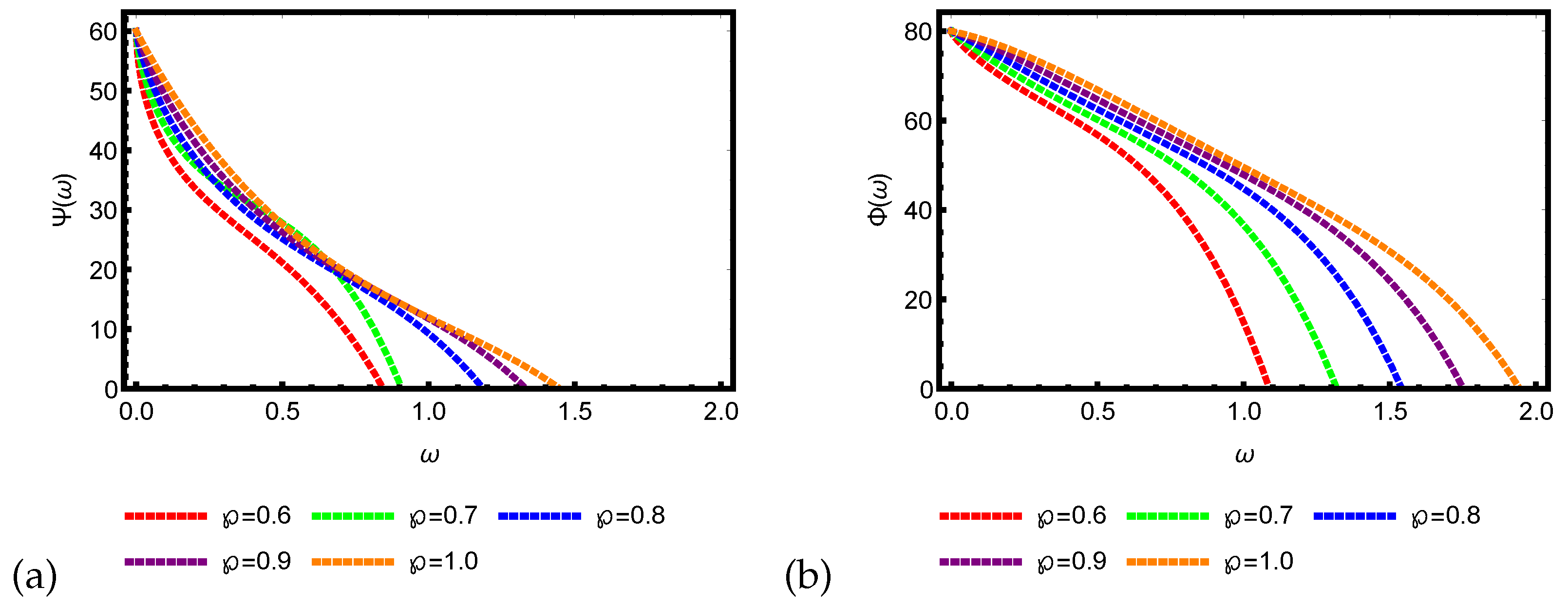
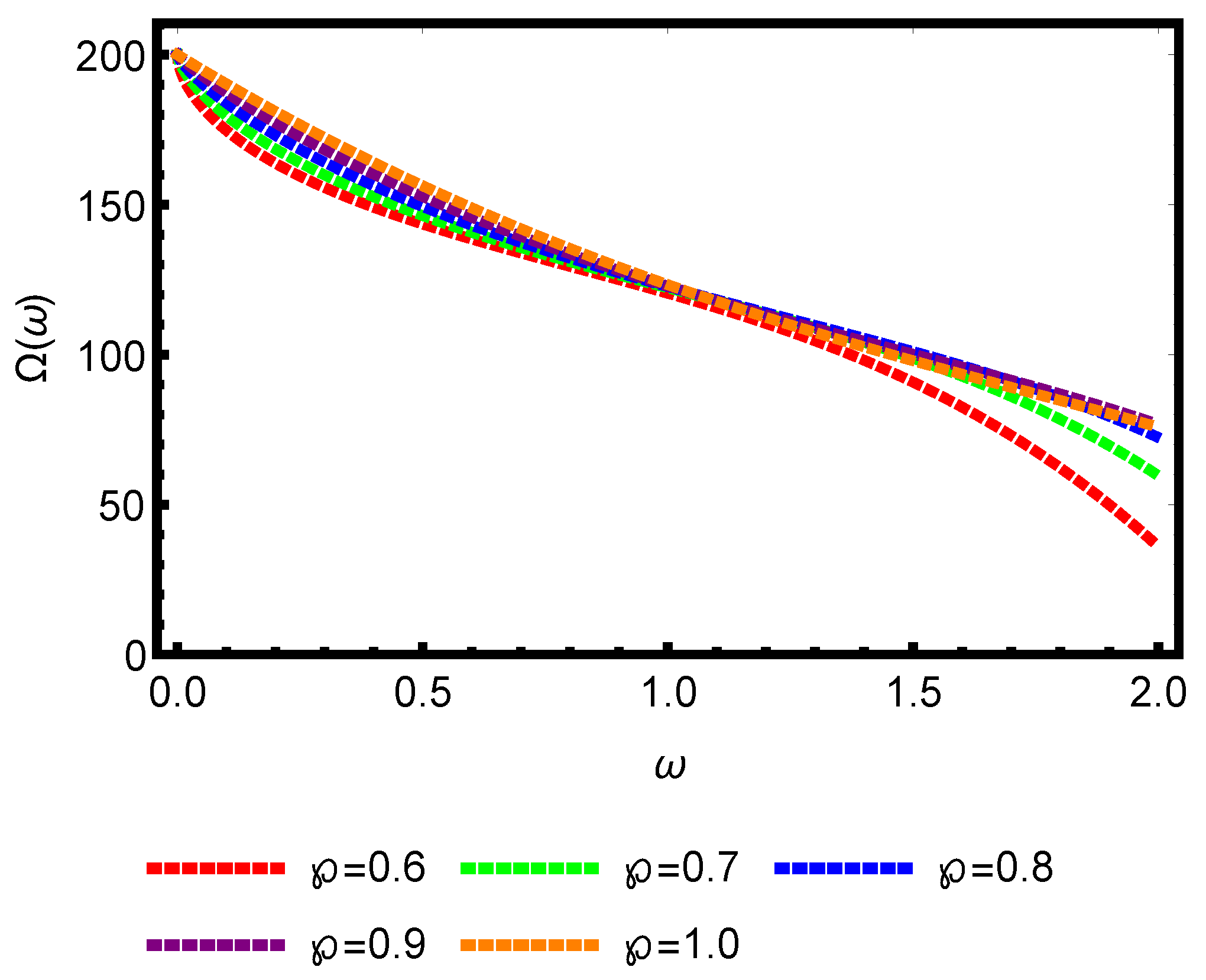
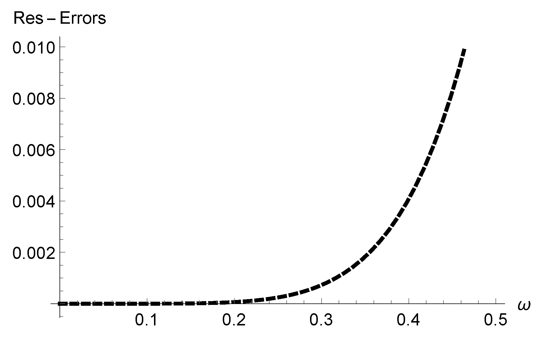
Figure 1, Figure 2 and Figure 3 illustrate the behaviors of the 6th-step App-Ss derived by ERPSM for potential smokers ϑ ( ω ) , light smokers Θ ( ω ) , smokers Ψ ( ω ) , quit smokers Φ ( ω ) , and total smokers Ω ( ω ) for various fractional derivative values, including = 0.6 , 0.7 , 0.8 , 0.9 , and 1.0 , within the interval ω [ 0 , 2.0 ] . From these figures, it is evident that the FNLSM exhibits a higher degree of freedom due to the utilization of fractional derivatives. The results show that the decline is significant for the lower fractional order but not as much for the higher order. It is important to note that we used a short period of time because we considered small initial values. The initial data should be sufficiently large for a longer time interval. Moreover, from these figures, we concluded that ERPSM yielded results that are in accordance with [25], which established the reliability and effectiveness of the suggested method for solving fractional nonlinear problems that arise in biological systems. Figure 4, Figure 5 and Figure 6 are used to assess the accuracy of the proposed method. These figures depict the Res-Errors obtained by the ERPSM for the FNLSM’s 6th-step App-Ss in the range ω [ 0 , 0.5 ] . For all sorts of smokers, we observed that the Res-Errors are incredibly small. We come to the conclusion that the proposed method provides a very accurate App-Ss in the form of a series. The convergence of the App-Ss to the exact solutions for FNLSM has been illustrated graphically using Rec-Errors in the interval ω [ 0 , 0.5 ] at = 1.0 , as shown in Figure 7, Figure 8, Figure 9, Figure 10 and Figure 11. These figures demonstrate that the suggested method quickly converges to the exact solutions because the Rec-Errors for the 5th-step App-Ss are very small, but they get even smaller for the 6th-step App-Ss. The Rec-Errors study confirmed the high level of convergence rates of App-Ss achieved by ERPSM. We therefore came to the conclusion that the proposed method is a practical and effective technique for solving nonlinear fractional models.
Table 1, Table 2, Table 3, Table 4 and Table 5 show how the 6th-step App-Ss of ϑ ( ω ) , Θ ( ω ) , Ψ ( ω ) , Φ ( ω ) and Ω ( ω ) obtained by ERPSM behave at different = 0.5 , 0.6 , 0.7 , 0.8 , 0.9 , and 1.0 FD values in the ω [ 0 , 1.0 ] interval. Table 6 and Table 7 show the Res-Errors for the 5th and 6th apps in the interval ω [ 0 , 0.5 ] as obtained by the ERPSM for the FNLSM at = 1.0 . From these tables, we observed that the Res-Errors for all the kinds of smokers in the 5th step App-Ss are very small. When we consider 6th-step App-Ss for all categories of smokers, the Rec-Errors become even smaller. This process of Rec-Errors shows the accuracy of our proposed method, and hence the approximation is rapidly converging to the exact solution. Table 8 and Table 9 compare the Res-errors of the third-step App-Ss derived by ERPSM and LDM [24] for all types of smokers in the ω [ 0 , 0.5 ] range. The results obtained using the proposed method show clear agreement with the LDM, confirming that the ERPSM is a useful substitute method in the solution of fractional nonlinear problems in biological systems.
In the following tables, we conduct a comparative study of our results obtained by ERPSM with those obtained by LDM [24] in the framework of Res-Errors. We observe that the results obtained by both methods are highly consistent with each other. Therefore, we conclude that ERPSM is an alternative method for solving NFDES in a straightforward manner.

5. Conclusions

In this research, we have utilized a novel straightforward approximate technique known as ERPSM to establish approximate series and numerical solutions for the FNLSM, which has held significant importance in applied sciences. The precision and convergence rates have been demonstrated through Res-Errors and Rec-Errors analyses, presented both graphically and numerically. ERPSM has proven to be a valuable alternative tool for solving fractional nonlinear models in biological systems, as evidenced by the outcomes demonstrating strong alignment with the LDM.
The advantages of ERPSM over other methods for providing approximate solutions, as evidenced by the results, can be summarized as follows: ERPSM determines the coefficients of terms of the series solution by applying the straightforward limit principle at zero. In contrast, other established methods like VIM, ADM, and HPM have necessitated integration, while RPSM has relied on derivatives, both of which have posed challenges in fractional contexts. Therefore, ERPSM is an alternative tool to various series solution methods for solving differential equations of fractional order. Moreover, ERPSM has been capable of solving NFDEs without relying on He’s or Adomian’s polynomials. Consequently, ERPSM has required significantly fewer computations to solve NFDEs, making it a viable substitute for methods reliant on He’s or Adomian polynomials. Additionally, ERPSM has generated series solutions for FNLSM without using the concepts of perturbation, linearization, or discretization, distinguishing it from numerous approximation techniques. Given these results, we have established that our technique is both accurate and simple to use.
In the future, we intend to employ ERPSM to solve both the Nagumo-type equation and evolutionary equations [34,35]. Additionally, we will investigate whether this method can be applied to stochastic problems. If any modifications are required for the method to solve fractional stochastic differential equations, we will work on implementing these amendments.

Author Contributions

Conceptualization, A.M.D., Z.A.K., M.I.L. and A.A.-Q.; methodology, A.M.D., Z.A.K., M.I.L. and A.A.-Q.; software, A.M.D., Z.A.K., M.I.L. and A.A.-Q.; validation, A.M.D., Z.A.K., M.I.L. and A.A.-Q.; formal analysis, A.M.D., Z.A.K., M.I.L. and A.A.-Q.; investigation, A.M.D., Z.A.K., M.I.L. and A.A.-Q.; resources, A.M.D. and Z.A.K.; writing—original draft preparation, A.M.D., Z.A.K. and M.I.L.; writing—review and editing, A.M.D., Z.A.K. and M.I.L.; visualization, A.M.D., Z.A.K. and M.I.L.; funding acquisition, A.M.D., Z.A.K. and A.A.-Q. All authors have read and agreed to the published version of the manuscript.

Funding

Princess Nourah bint Abdulrahman University Researchers Supporting Project number (PNURSP2024R8). Princess Nourah bint Abdulrahman University, Riyadh, Saudi Arabia. This work was supported by the Deanship of Scientific Research, Vice Presidency for Graduate Studies and Scientific Research, King Faisal University, Saudi Arabia (Project No. GrantA191).

Data Availability Statement

The article contained both data and implementing information.

Conflicts of Interest

The authors declare no conflicts of interest.

Appendix A

The detailed derivations of ϑ 1 , Θ 1 , Ψ 1 , Φ 1 , and Ω 1 are given below.
Firstly, by utilizing κ = 1 in Equation (13) and κ th-truncated FPS, we obtain the following results:
Z R e s 1 ( ϑ * ( σ ) ) = ϑ 1 * ( σ ) σ 2 ϑ 0 σ β Ω 1 * ( σ ) + σ δ 1 Z Z 1 [ ϑ 1 * ( σ ) ] Z 1 [ Θ 1 * ( σ ) ] + σ ( ζ 1 + ϖ ) ϑ 1 * ( σ ) σ θ Φ 1 * ( σ ) , Z R e s 1 ( Θ * ( σ ) ) = Θ 1 * ( σ ) σ 2 Θ 0 + σ δ 1 Z Z 1 [ ϑ 1 * ( σ ) ] Z 1 [ Θ 1 * ( σ ) ] + σ δ 2 Z Z 1 [ Ψ 1 * ( σ ) ] Z 1 [ Θ 1 * ( σ ) ] + ( ζ 2 + ϖ ) σ Θ 1 * ( σ ) , Z R e s 1 ( Ψ * ( σ ) ) = Ψ 1 * ( σ ) σ 2 Ψ 0 σ δ 2 Z Z 1 [ Ψ 1 * ( σ ) ] Z 1 [ Θ 1 * ( σ ) ] + σ ( Y + ζ 3 + ϖ ) Ψ 1 * ( σ ) , Z R e s 1 ( Φ * ( σ ) ) = Φ 1 * ( σ ) σ 2 Φ 0 σ Y Ψ 1 * ( σ ) + σ ( θ ζ 4 + ϖ ) Φ 1 * ( σ ) , Z R e s 1 ( Ω * ( σ ) ) = Ω 1 * ( σ ) σ 2 Ω 0 + σ ( β ϖ ) Ω 1 * ( σ ) + σ ζ 1 ϑ 1 * ( σ ) + ζ 2 Θ 1 * ( σ ) ζ 3 Ψ 1 * ( σ ) + ζ 4 Φ 1 * ( σ ) .
Further, ϑ 1 * ( σ ) = ϑ 0 σ 2 + ϑ 1 σ 2 + ,   Θ 1 * ( σ ) = Θ 0 σ 2 + Θ 1 σ 2 + ,   Ψ 1 * ( σ ) = Ψ 0 σ 2 + Ψ 1 σ 2 + ,   Φ 1 * ( σ ) = Φ 0 σ 2 + Φ 1 σ 2 + , and Ω 1 * ( σ ) = Ω 0 σ 2 + Ω 1 σ 2 + ,
By utilizing the above-obtained results, we obtain the following outcomes:
e q ( A 2 ) Z R e s 1 ( ϑ * ( σ ) ) = ϑ 0 σ 2 + ϑ 1 σ 2 + ϑ 0 σ 2 σ β Ω 0 σ 2 + Ω 1 σ 2 + + σ δ 1 Z [ Z 1 [ ϑ 0 σ 2 + ϑ 1 σ 2 + ] Z 1 [ Θ 0 σ 2 + Θ 1 σ 2 + ] ] + σ ( ζ 1 + ϖ ) ϑ 0 σ 2 + ϑ 1 σ 2 + σ θ Φ 0 σ 2 + Φ 1 σ 2 + , Z R e s 1 ( Θ * ( σ ) ) = Θ 0 σ 2 + Θ 1 σ 2 + σ 2 Θ 0 + σ δ 1 Z Z 1 [ ϑ 0 σ 2 + ϑ 1 σ 2 + ] Z 1 [ Θ 0 σ 2 + Θ 1 σ 2 + + σ δ 2 Z Z 1 [ Ψ 0 σ 2 + Ψ 1 σ 2 + ] Z 1 [ Θ 0 σ 2 + Θ 1 σ 2 + ] + ( ζ 2 + ϖ ) σ Θ 0 σ 2 + Θ 1 σ 2 + , Z R e s 1 ( Ψ * ( σ ) ) = Ψ 0 + Ψ 1 σ 2 + σ 2 Ψ 0 σ δ 2 Z Z 1 [ Ψ 0 σ 2 + Ψ 1 σ 2 + ] Z 1 [ Θ 0 + Θ 1 σ 2 + ] + σ ( Y + ζ 3 + ϖ ) Ψ 0 σ 2 + Ψ 1 σ 2 + , Z R e s 1 ( Φ * ( σ ) ) = Φ 0 σ 2 + Φ 1 σ 2 + σ 2 Φ 0 σ Y Ψ 0 σ 2 + Ψ 1 σ 2 + + σ ( θ ζ 4 + ϖ ) Φ 0 σ 2 + Φ 1 σ 2 + , Z R e s 1 ( Ω * ( σ ) ) = Ω 0 σ 2 + Ω 1 σ 2 + σ 2 Ω 0 + σ ( β ϖ ) Ω 0 σ 2 + Ω 1 σ 2 + + σ ( ζ 1 ϑ 0 σ 2 + ϑ 1 σ 2 + + ζ 2 Θ 0 σ 2 + Θ 1 σ 2 + ζ 3 Ψ 0 σ 2 + Ψ 1 σ 2 + + ζ 4 Φ 0 σ 2 + Φ 1 σ 2 + ) .
By using values of Z R e s 1 ( ϑ * ( σ ) ) , Z R e s 1 ( Θ * ( σ ) ) , Z R e s 1 ( Ψ * ( σ ) ) , Z R e s 1 ( Φ * ( σ ) ) , and Z R e s 1 ( Ω * ( σ ) ) in Equation (14), we obtain the desired values of ϑ 1 , Θ 1 , Ψ 1 , Φ 1 , and Ω 1 , as provided in Equation (15). In the same way, we obtained the remaining coefficient of FPS by repeating the procedure for κ = 2 , 3 , 4 , 5 , and 6. The values are provided in Equations (16)–(20).

References

  1. Monje, C.A.; Chen, Y.; Vinagre, B.M.; Xue, D.; Feliu-Batlle, V. Fractional-Order Systems and Controls: Fundamentals and Applications; Springer Science Business Media: Berlin/Heidelberg, Germany, 2010. [Google Scholar]
  2. Samko, S. Fractional integration and differentiation of variable order: An overview. Nonlinear Dyn. 2013, 71, 653–662. [Google Scholar] [CrossRef]
  3. Abu-Ghuwaleh, M.; Saadeh, R. New definitions of fractional derivatives and integrals for complex analytic functions. Arab. J. Basic Appl. Sci. 2023, 30, 675–690. [Google Scholar] [CrossRef]
  4. Zhou, P.; Ma, J.; Tang, J. Clarify the physical process for fractional dynamical systems. Nonlinear Dyn. 2020, 100, 2353–2364. [Google Scholar] [CrossRef]
  5. Arfan, M.; Lashin, M.M.; Sunthrayuth, P.; Shah, K.; Ullah, A.; Iskakova, K.; Abdeljawad, T. On nonlinear dynamics of COVID-19 disease model corresponding to nonsingular fractional order derivative. Med. Biol. Eng. Comput. 2022, 60, 3169–3185. [Google Scholar] [CrossRef] [PubMed]
  6. Mangal, S.; Misra, O.P.; Dhar, J. SIRS epidemic modeling using fractional-ordered differential equations: Role of fear effect. Int. J. Biomath. 2024, 17, 2350044. [Google Scholar] [CrossRef]
  7. Singh, H.; Baleanu, D.; Singh, J.; Dutta, H. Computational study of fractional order smoking model. Chaos Solit. Fract. 2021, 142, 110440. [Google Scholar] [CrossRef]
  8. Alrabaiah, H.; Zeb, A.; Alzahrani, E.; Shah, K. Dynamical analysis of fractional-order tobacco smoking model containing snuffing class. Alex. Eng. J. 2021, 60, 3669–3678. [Google Scholar] [CrossRef]
  9. Hassani, H.; Machado, J.T.; Avazzadeh, Z.; Naraghirad, E.; Mehrabi, S. Optimal solution of the fractional-order smoking model and its public health implications. Nonlinear Dyn. 2022, 108, 2815–2831. [Google Scholar] [CrossRef]
  10. Liu, P.; Munir, T.; Cui, T.; Din, A.; Wu, P. Mathematical assessment of the dynamics of the tobacco smoking model: An application of fractional theory. AIMS Math. 2022, 7, 7143–7165. [Google Scholar] [CrossRef]
  11. Swartz, J.B. Use of a Multistage Model to Predict Time Trends in Smoking Induced Lung Cancer. J. Epidemiol. Community Health 1992, 46, 311–315. [Google Scholar] [CrossRef]
  12. Brauer, F.; Castillo-Cha’vez, C. Mathematical Models in Population Biology and Epidemiology; Springer: Berlin/Heidelberg, Germany, 2001. [Google Scholar]
  13. Zaman, G. Optimal campaign in the smoking dynamics. Comput. Math. Methods Med. 2011, 2011, 163834. [Google Scholar] [CrossRef]
  14. Li, C.; Zhang, H.; Yang, X. A New Nonlinear Compact Difference Scheme for a Fourth-Order Nonlinear Burgers Type Equation with a Weakly Singular Kernel. J. Appl. Math. Comput. 2024, 2024, 1–33. [Google Scholar] [CrossRef]
  15. Shi, Y.; Yang, X. Pointwise error estimate of conservative difference scheme for supergeneralized viscous Burgers’ equation. Electron. Res. Arch. 2024, 32, 1471–1497. [Google Scholar] [CrossRef]
  16. Wang, W.; Zhang, H.; Zhou, Z.; Yang, X. A Fast Compact Finite Difference Scheme for the Fourth-Order Diffusion-Wave Equation. Inter. J. Comput. Math. 2024, 101, 170–193. [Google Scholar] [CrossRef]
  17. Shi, Y.; Yang, X. A time two-grid difference method for nonlinear generalized viscous Burgers’ equation. J. Math. Chem. 2024, 2014, 1–34. [Google Scholar] [CrossRef]
  18. Liaqat, M.I.; Khan, A.; Akgül, A. Adaptation on power series method with conformable operator for solving fractional order systems of nonlinear partial differential equations. Chaos Solit. Fract. 2022, 157, 111984. [Google Scholar] [CrossRef]
  19. Zaky, M.A. An accurate spectral collocation method for nonlinear systems of fractional differential equations and related integral equations with nonsmooth solutions. Appl. Numer. Math. 2020, 154, 205–222. [Google Scholar] [CrossRef]
  20. Jajarmi, A.; Baleanu, D. A new iterative method for the numerical solution of high-order non-linear fractional boundary value problems. Front. Phys. 2020, 8, 220. [Google Scholar] [CrossRef]
  21. Khalid, N.; Abbas, M.; Iqbal, M.K.; Singh, J.; Ismail, A.I.M. A computational approach for solving time fractional differential equation via spline functions. Alex. Eng. J. 2020, 59, 3061–3078. [Google Scholar] [CrossRef]
  22. Babaei, A.; Jafari, H.; Banihashemi, S. Numerical solution of variable order fractional nonlinear quadratic integro-differential equations based on the sixth-kind Chebyshev collocation method. J. Comput. Appl. Math. 2020, 377, 112908. [Google Scholar] [CrossRef]
  23. Li, D.; Sun, W.; Wu, C. A novel numerical approach to time-fractional parabolic equations with nonsmooth solutions. Numer. Math. Theory Methods Appl. 2021, 14, 355–376. [Google Scholar]
  24. Haq, F.; Shah, K.; ur Rahman, G.; Shahzad, M. Numerical solution of fractional order smoking model via Laplace Adomian decomposition method. Alex. Eng. J. 2018, 57, 1061–1069. [Google Scholar] [CrossRef]
  25. Mahdy, A.M.S.; Sweilam, N.H.; Higazy, M. Approximate solution for solving nonlinear fractional order smoking model. Alex. Eng. J. 2020, 59, 739–752. [Google Scholar] [CrossRef]
  26. Pavani, K.; Raghavendar, K. A novel technique to study the solutions of time fractional nonlinear smoking epidemic model. Sci. Rep. 2024, 14, 4159. [Google Scholar] [CrossRef] [PubMed]
  27. Khan, S.A.; Shah, K.; Zaman, G.; Jarad, F. Existence Theory and Numerical Solutions to Smoking Model under Caputo-Fabrizio Fractional Derivative. Chaos: An Interdiscip. J. Nonlinear Sci. 2019, 29, 013128. [Google Scholar]
  28. Veeresha, P.; Prakasha, D.G.; Baskonus, H.M. Solving smoking epidemic model of fractional order using a modified homotopy analysis transform method. Math. Sci. 2019, 13, 115–128. [Google Scholar] [CrossRef]
  29. Gunerhan, H.; Rezazadeh, H.; Adel, W.; Hatami, M.; Sagayam, K.M.; Emadifar, H.; Hamoud, A.A. Analytical approximate solution of fractional order smoking epidemic model. Adv. Mech. Eng. 2022, 14, 1–11. [Google Scholar]
  30. Mohammed, O.H.; Salim, H.A. Computational methods based laplace decomposition for solving nonlinear system of fractional order differential equations. Alex. Eng. J. 2018, 57, 3549–3557. [Google Scholar] [CrossRef]
  31. He, W.; Chen, N.; Dassios, I.; Shah, N.A.; Chung, J.D. Fractional system of Korteweg-De Vries equations via Elzaki transform. Mathematics 2021, 9, 673. [Google Scholar] [CrossRef]
  32. Liaqat, M.I.; Akgül, A.; Bayram, M. Series and Closed Form Solution of Caputo Time-Fractional Wave and Heat Problems with the Variable Coefficients by a Novel Approach. Opt. Quant. Electron. 2024, 56, 203. [Google Scholar] [CrossRef]
  33. Liaqat, M.I.; Khan, A.; Akgül, A.; Ali, M.S. A Novel Numerical Technique for Fractional Ordinary Differential Equations with Proportional Delay. J. Funct. Spaces 2022, 2022, 1–21. [Google Scholar] [CrossRef]
  34. Yang, X.; Zhang, Z. On conservative, positivity preserving, nonlinear FV scheme on distorted meshes for the multi-term nonlocal Nagumo-type equations. Appl. Math. Lett. 2024, 150, 108972. [Google Scholar] [CrossRef]
  35. Yang, X.; Qiu, W.; Chen, H.; Zhang, H. Second-order BDF ADI Galerkin finite element method for the evolutionary equation with a nonlocal term in three-dimensional space. Appl. Numer. Math. 2022, 172, 497–513. [Google Scholar] [CrossRef]
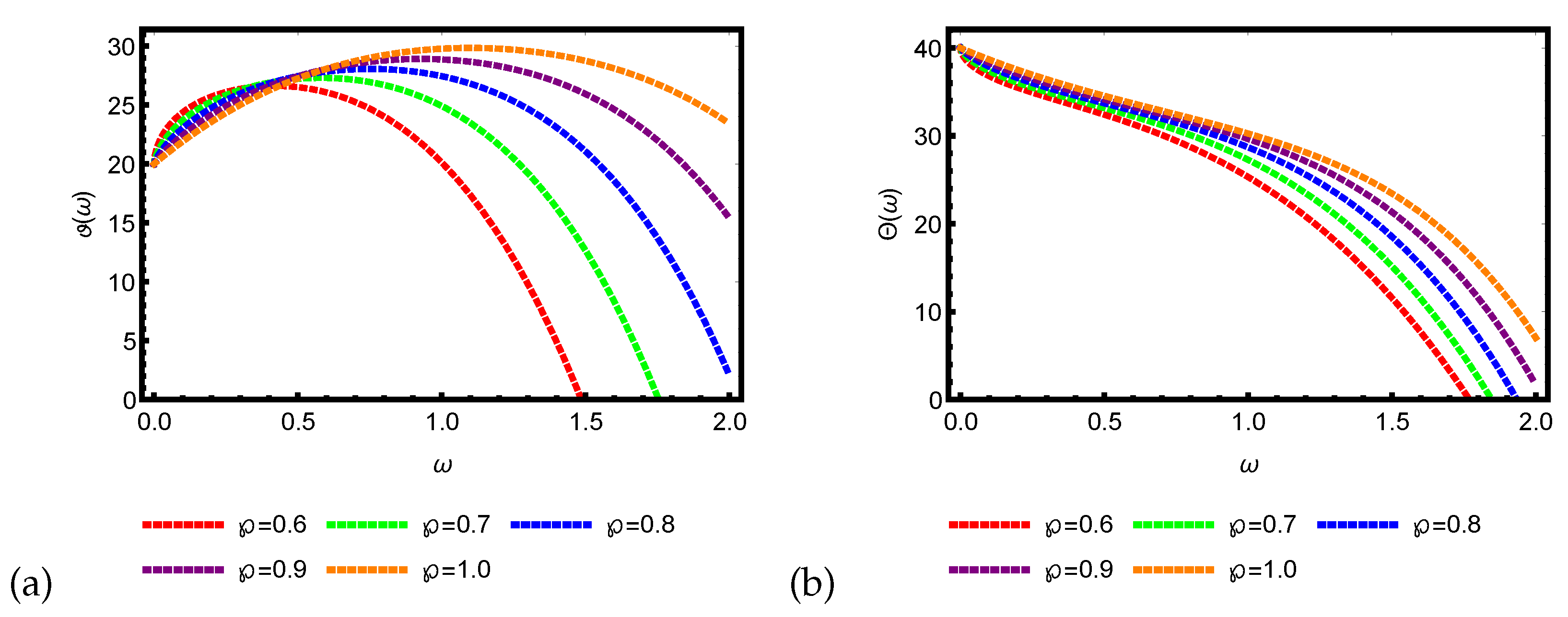
Figure 1. The behavior of 6th-step App-Ss with = 0.6 , 0.7 , 0.8 , 0.9 , 1.0 of (a) potential smokers, ϑ ( ω ) ; (b) light smokers, Θ ( ω ) .
Fractalfract 08 00286 g001
Figure 2. The behavior of 6th-step App-Ss with = 0.6 , 0.7 , 0.8 , 0.9 , 1.0 of (a) smokers, Ψ ( ω ) ; (b) quit smokers, Φ ( ω ) .
Fractalfract 08 00286 g002
Figure 3. The behavior of 6th-step App-S with = 0.6 , 0.7 , 0.8 , 0.9 , 1.0 of total smokers, Ω ( ω ) .
Fractalfract 08 00286 g003
Figure 4. The Res-Errors of 6th-step App-Ss are as follows: (a) potential smokers, ϑ ( ω ) ; (b) light smokers, Θ ( ω ) at = 1.0 .
Fractalfract 08 00286 g004
Figure 5. The Res-Errors of 6th-step App-Ss are as follows: (a) smokers, Ψ ( ω ) ; (b) quit smokers, Φ ( ω ) at = 1.0 .
Fractalfract 08 00286 g005
Figure 6. The Res-Errors of 6th-step App-S for total smokers Ω ( ω ) .
Fractalfract 08 00286 g006
Figure 7. Graphs of Rec-Errors in the interval ω [ 0 , 0.5 ] when = 1.0 : (a) | ϑ 5 ( ω ) ϑ 4 ( ω ) | , (b) | ϑ 6 ( ω ) ϑ 5 ( ω ) | .
Fractalfract 08 00286 g007
Figure 8. Graphs of Rec-Errors in the interval ω [ 0 , 0.5 ] when = 1.0 : (a) | Θ 5 ( ω ) Θ 4 ( ω ) | , (b) | Θ 6 ( ω ) Θ 5 ( ω ) | .
Fractalfract 08 00286 g008
Figure 9. Graphs of Rec-Errors in the interval ω [ 0 , 0.5 ] when = 1.0 : (a) | Ψ 5 ( ω ) Ψ 4 ( ω ) | , (b) | Ψ 6 ( ω ) ψ 5 ( ω ) | .
Fractalfract 08 00286 g009
Figure 10. Graphs of Rec-Errors in the interval ω [ 0 , 0.5 ] when = 1.0 : (a) | Φ 5 ( ω ) Φ 4 ( ω ) | , (b) | Φ 6 ( ω ) Φ 5 ( ω ) | .
Fractalfract 08 00286 g010
Figure 11. Graphs of Rec-Errors in the interval ω [ 0 , 0.5 ] when = 1.0 : (a) | Ω 5 ( ω ) Ω 4 ( ω ) | , (b) | Ω 6 ( ω ) Ω 5 ( ω ) | .
Fractalfract 08 00286 g011
Table 1. ϑ ( ω ) behavior at various values.
ω = 0.6 = 0.7 = 0.8 = 0.9 = 1.0
0.1 24.3750 23.6971 23.0343 28.8668 21.9131
0.2 25.7061 25.2921 24.7592 28.8668 23.581
0.3 26.3695 26.2781 25.9725 28.8668 25.0176
0.4 26.6172 26.8904 26.8427 28.8668 26.2374
0.5 26.5161 27.2191 27.4509 28.8668 27.2551
0.6 26.0702 27.2979 27.8413 28.8668 28.0848
0.7 25.2547 27.1300 28.0358 28.8668 28.7407
0.8 24.0291 26.6996 28.0411 28.8668 29.235
0.9 22.3432 25.9767 27.8513 28.8668 29.5787
1.0 20.1403 24.9207 27.4504 28.8668 29.7803
Table 2. Θ ( ω ) behavior at various values.
ω = 0.6 = 0.7 = 0.8 = 0.9 = 1.0
0.1 36.7931 37.3704 37.8765 38.3126 38.6792
0.2 35.4676 36.0428 36.5635 37.0484 37.4978
0.3 34.4138 35.0008 35.505 35.976 36.4312
0.4 33.4292 34.0719 34.5765 35.0243 35.4555
0.5 32.4207 33.1699 33.7091 34.1473 34.5495
0.6 31.3302 32.2363 32.8527 33.3081 33.6915
0.7 30.1124 31.2237 31.9646 32.4733 32.8593
0.8 28.7286 30.089 31.0045 31.6097 32.0283
0.9 27.1437 28.7909 29.9319 30.6825 31.1727
1.0 25.3242 27.2881 28.7046 29.6542 30.2621
Table 3. Ψ ( ω ) behavior at various values.
ω = 0.6 = 0.7 = 0.8 = 0.9 = 1.0
0.1 40.3498 43.4776 46.4251 49.0826 51.3815
0.2 33.6865 36.1773 38.7503 41.3893 43.9953
0.3 31.3447 31.1612 33.1467 35.3161 37.6663
0.4 25.1759 27.2493 28.7682 30.3769 32.2422
0.5 21.1535 23.8488 25.1668 26.2779 27.5896
0.6 16.5328 20.5494 22.0337 22.8044 23.5891
0.7 10.884 17.0038 19.1155 19.7788 20.1306
0.8 3.81331 12.8878 16.1771 17.0388 17.1088
0.9 0.0000 7.87628 12.9823 14.4238 14.4184
1.0 0.0000 1.6342 9.28190 11.7653 11.9495
Table 4. Φ ( ω ) behavior at various values.
ω = 0.6 = 0.7 = 0.8 = 0.9 = 1.0
0.1 73.2326 75.1508 76.5721 77.5862 78.2947
0.2 68.6195 70.9958 73.0208 74.6795 75.9829
0.3 64.6459 67.1806 69.4402 71.4721 73.2252
0.4 60.8445 63.6189 65.9297 68.1171 70.1529
0.5 56.7892 60.1818 62.5195 64.7121 66.8716
0.6 52.0247 56.6919 59.1907 61.3152 63.465
0.7 46.0478 52.9183 55.8813 57.9519 59.9966
0.8 38.2974 48.5693 52.4854 54.6175 56.5105
0.9 28.1516 43.2892 48.8494 51.2765 53.0316
1.0 14.9268 36.6506 44.7664 47.8593 50.0316
Table 5. Ω ( ω ) behavior at various values.
ω = 0.6 = 0.7 = 0.8 = 0.9 = 1.0
0.1 174.7853 179.7025 183.9093 187.4144 190.2682
0.2 163.7824 168.5715 173.1086 177.2942 181.0585
0.3 155.7041 159.8945 164.13322 168.3195 172.3465
0.4 149.1545 152.6465 156.3363 160.1892 164.1075
0.5 143.5553 146.3673 149.4094 152.7442 156.3195
0.6 138.5483 140.7923 143.1632 145.8825 148.9592
0.7 133.9145 135.7273 137.4642 139.5225 142.0012
0.8 129.4625 131.0385 132.2115 133.6035 135.4255
0.9 125.0315 126.5975 127.3175 128.0733 129.2065
1.0 121.0312 122.5973 123.3175 122.0735 139.2463
Table 6. The Rec-Errors for the App-Ss in the 5th and 6th iterations for ϑ ( ω ) , Θ ( ω ) , and Ψ ( ω ) .
ω Rec - Errors Rec - Errors Rec - Errors Rec - Errors Rec - Errors Rec - Errors
| ϑ ( 5 ) ϑ ( 4 ) | | ϑ ( 6 ) ϑ ( 5 ) | | Θ ( 5 ) Θ ( 4 ) | | Θ ( 6 ) Θ ( 5 ) | | Ψ ( 5 ) Ψ ( 4 ) | | Ψ ( 6 ) Ψ ( 5 ) |
0.1 0.00000393774 0.00000010258 0.00000800088 0.00000032878 0.00003876801 0.00000082414
0.2 0.00012600801 0.00000656485 0.00025602801 0.00002104160 0.00124058012 0.00005274521
0.3 0.00095687100 0.00007477780 0.00194421001 0.00023967701 0.00942063101 0.00060080102
0.4 0.00403225001 0.00042015101 0.00819290001 0.00134666021 0.03969840102 0.00337569001
0.5 0.01230540120 0.00160275001 0.02500270012 0.00513711011 0.12115110001 0.01287730011
Table 7. The Rec-Errors for the App-Ss in the 5th and 6th iterations for Φ ( ω ) and Ω ( ω ) .
ω Rec - Errors Rec - Errors Rec - Errors Rec - Errors
| Φ ( 5 ) Φ ( 4 ) | | Φ ( 6 ) Φ ( 5 ) | | Ω ( 5 ) Ω ( 4 ) | | Ω ( 6 ) Ω ( 5 ) |
0.1 0.00005812280 0.000001521201 0.00000567675 0.00000019891
0.2 0.00185993010 0.000097356900 0.00018165601 0.00001273060
0.3 0.01412380001 0.00110896002 0.00137945001 0.00014501001
0.4 0.05951770003 0.006230840010 0.00581299002 0.00081476002
0.5 0.18163410201 0.02376880001 0.01773981020 0.00310806003
Table 8. The comparison of Res-Errors in 3rd-step App-Ss of ϑ ( ω ) , Θ ( ω ) , and Ψ ( ω ) obtained by ERPSM and SDM.
ω Res - Errors Res - Errors Res - Errors Res - Errors Res - Errors Res - Errors
[ ϑ ( ω ) ] [ ERPSM ] [ ϑ ( ω ) ] [ LDM ] [ Θ ( ω ) ] [ ERPSM ] [ Θ ( ω ) ] [ LDM ] [ Ψ ( ω ) ] [ ERPSM ] [ Ψ ( ω ) ] [ LDM ]
0.1 0.00295059101 0.00295059101 0.00896119120 0.00896119120 0.00797612010 0.00797612010
0.2 0.02532571201 0.02532571201 0.06905251122 0.06905251122 0.00440025120 0.00440025120
0.3 0.09087270012 0.09087270012 0.224824110011 0.224824110011 0.00055981812 0.00055981812
0.4 0.22726811220 0.22726811220 0.51490300001 0.51490300001 0.00326328012 0.00326328012
0.5 0.46531721210 0.46531721210 0.97319521210 0.97319521210 0.01277340001 0.01277340001
Table 9. The comparison of Res-Errors in 3rd-step App-Ss of Φ ( ω ) and Ω ( ω ) obtained by ERPSM and SDM.
ω Res - Errors Res - Errors Res - Errors Res - Errors
[ Φ ( ω ) ] [ ERPSM ] [ Φ ( ω ) ] [ LDM ] [ Ω ( ω ) ] [ ERPSM ] [ Ω ( ω ) ] [ LDM ]
0.1 0.00290541001 0.00290541001 0.00028394910 0.00028394910
0.2 0.00464952002 0.00464952002 0.00454189120 0.00454189120
0.3 0.02353910210 0.02353910210 0.02299221120 0.02299221120
0.4 0.07439590211 0.07439590211 0.07266461101 0.07266461101
0.5 0.81632002110 0.81632002110 0.17740211210 0.17740211210
Disclaimer/Publisher’s Note: The statements, opinions and data contained in all publications are solely those of the individual author(s) and contributor(s) and not of MDPI and/or the editor(s). MDPI and/or the editor(s) disclaim responsibility for any injury to people or property resulting from any ideas, methods, instructions or products referred to in the content.