Non-Extensive Statistical Analysis of Seismicity on the West Coastline of Mexico

Abstract

Mexico is a well-known seismically active country, which is primarily affected by several tectonic plate interactions along the southern Pacific coastline and by active structures in the Gulf of California. In this paper, we investigate this seismicity using the classical Gutenberg–Richter (GR) law and a non-extensive statistical approach based on Tsallis entropy. The analysis is performed using data from the corrected Mexican seismic catalog provided by the National Seismic Service, spanning the period from January 2000 to October 2023, and unlike previous work, it includes six different regions along the entire west coastline of Mexico. The Gutenberg–Richter law fitting to the earthquake sub-catalogs for all six regions studied indicates magnitudes of completeness between 3.30 and 3.76, implying that the majority of seismic movements occur for magnitudes less than 4. The cumulative distribution of earthquakes as derived from the Tsallis entropy was fitted to the corrected catalog data to estimate the q-entropic index for all six regions, which for values greater than one is a measure of the non-extensivity (i.e., non-equilibrium) of the system. All regions display values of the entropic index in the range $1.52\lesssim q\lesssim 1.61$, slightly lower than previously estimated ( $1.54\lesssim q\lesssim 1.70$) using catalog data from 1988 to 2010. The reason for this difference is related to the use of modern recording devices, which are sensitive to the detection of a larger number of low-magnitude events compared to older instrumentation.

1. Introduction

Non-extensive statistical mechanics (NESM) based on Tsallis formalism [1,2,3] represents a robust theoretical framework for the description and interpretation of non-equilibrium complex systems, including real seismicity, faulting, and plate tectonics, with a special focus on the mechanism(s) of earthquake generation. Since earthquakes are often catastrophic events, understanding their physics is a mandatory aspect of research in seismology and of high priority in many seismically active countries.

In particular, Tsallis’ NESM, or q-statistics, is a generalization of the Boltzmann–Gibbs (BG) statistics with additive entropy into an NESM with a non-additive entropy function that allows the description of physical processes involving long-range interactions, long-term memories, and multifractal properties [4]. In contrast to GB thermodynamics, a non-additive entropy was indeed necessary to account for correlations between different elements of the system at all length scales. Such correlations lead to broad distributions with a power-law asymptotic behavior. For a detailed description of Tsallis’ theory the interested reader is referred to papers and books in Refs. [2,3,5,6,7]. Since its development, NESM has been applied to the analysis of the macroscopic properties of earthquakes at both regional [8,9] and global scales [10]. In a seminal paper, Sotolongo-Costa and Posadas [11] developed a model for the physical mechanism of earthquake triggering—the so-called fragment–asperity model, based on the interaction between the fragments, generated by the local breaking of the tectonic plates, and the asperity of the fault planes. Since then, a growing number of papers dealing with the analysis of seismicity, plate tectonics, and precursory electromagnetic anomalies in different regions around the world have been devoted to demonstrating the consistency between NESM and observations. The Sotolongo-Costa and Posadas [11] model for earthquake magnitudes was extended by Silva et al. [12] to include a relationship between the volumetric fragment size and the earthquake energy, which appears to be more consistent with the standard theory of seismic moment [13]. This improved formulation leads to a different earthquake magnitude distribution compared to Sotolongo-Costa and Posadas’s model and it was found to fit equally well the magnitude distribution of several regional seismicities and local seismic zones around the world [14,15,16,17,18,19,20,21,22,23].

Mexico’s seismicity is due to the fact that the country lies on the eastern rim of the Ring of Fire, where a large number of seismic events and volcanic eruptions occur in the basin of the Pacific Ocean. The country is particularly affected by the interaction between the Cocos Plate and the North American Plate. Such tectonic plate interactions are responsible for the fragmentation of the Earth’s crust, which is the likely mechanism for triggering earthquakes. In particular, the seismicity of Mexico has been previously studied by a number of authors during the past four decades [19,24,25,26,27,28,29,30,31,32,33,34,35]. A natural time analysis of six tectonic zones in the Mexican Pacific coast revealed that extreme events could be expected in the Chiapas region [34]. Most recent analyses of the Mexican seismicity are, therefore, related to the deadly M8.2 earthquake [34,35], which was one of the largest Mexican seismic events. In this case, a precursory behavior three months before the occurrence of the M8.2 earthquake in Chiapas was identified using natural time [35], which was related to fluctuations in the entropy change under time reversal and an abrupt simultaneous increase in the Tsallis q-entropic index [34]. In particular, a non-extensive analysis of the seismicity in Mexico based on Tsallis’ q-statistics between 1988 and 2010 along the South Pacific coast, including the regions of Jalisco, Michoacán, Guerrero, and Oaxaca, was performed by Valverde-Esparza et al. [19]. These four regions are characterized by different subduction patterns, and therefore, by different tectonic regimes. They obtained q-values well in the range of those derived for other regions reported in the literature. For example, for the Jalisco region their analysis yielded $q=1.7020$ against $q=1.6845$, 1.6635, and 1.6370 for the Michoacán, Oaxaca, and Guerrero regions, respectively. Since lower values of q indicate more stability, it was concluded that the subduction zone is more unstable on the northwestern coastline (Jalisco) than on the southeastern part (Guerrero and Oaxaca). These results are indicative of a possible correlation between the seismicity pattern associated with the inclination angle of each subduction zone and the value of the non-extensive parameter q.

In this paper, the frequency–magnitude distribution of earthquakes along the entire Pacific coast of Mexico from the Gulf of California to Chiapas is investigated in the framework of the classical Gutenberg–Richter (GR) relation and the non-extensive model for earthquakes revisited by Silva et al. [12]. The investigated seismicity includes six tectonic zones and the period analyzed spans from 1 January 2000 to 13 October 2023, as provided in the corrected Mexican seismic catalog provided by the National Seismic Service (http://www.ssn.unam.mx, accessed on 20 April 2024). Novel aspects of the present research include the non-extensive analysis of the seismicity of the Gulf of California. While the Sotolongo-Costa and Posadas model is well suited to study rock fragmentation at the interface of subducting plates, here the model is used for the first time in the analysis of dispersion zones, as is the case for the seismicity in the Gulf of California. In addition, the corrected catalog includes the records of telluric events from a new seismic monitoring network consisting of broadband sensors disseminated along the entire Pacific coast of Mexico. Compared to previous work the period analyzed is longer and includes the last 20 years, while the use of more sensitive instruments improves the quality of the data, and therefore, the estimation of the q-entropic indices. On the other hand, as detailed at the end of Section 4, two efficient and less time-consuming optimization algorithms were employed to obtain the minimum-error fitting to the observed data. This paper is organized as follows. Section 2 is devoted to a brief description of NESM based on Tsallis entropy along with Silva et al.’s [12] non-extensive model for the earthquake energy distribution function and cumulative number of earthquakes. The tectonic setting is briefly described in Section 3, while the dataset description and analysis procedure are discussed in Section 4. Section 5 describes the results obtained and Section 6 summarizes the relevant conclusions.

2. Non-Extensive Statistical Mechanics

2.1. Non-Additive Tsallis Entropy and Probability Distribution

The integral formulation of the non-additive Tsallis entropy, $S_q$, for a continuous variable $\sigma \in \mathbb{R}$ can be written as [4]

$$S_q\left(\sigma \right)=\frac{k_{\mathrm{B}}}{q-1}\left[1-{\int }_0^{\infty }{p}^q\left(\sigma \right)d\sigma \right],$$

(1)

where $k_{\mathrm{B}}$ is the Boltzmann constant, $q\in \mathbb{R}$ is the non-extensive parameter (or entropic index), and $\sigma$ stands for a dimensionless characteristic surface of a fragment. In the Sotolongo-Costa and Posadas [11] model, $p\left(\sigma \right)$ is a probability distribution function referred to as the size distribution function of the fragments. In particular, Sotolongo-Costa and Posadas [11] define $p\left(\sigma \right)$ as the probability density of finding a fragment of the relative dimensionless surface $\sigma$. In the limit $q\to 1$, Equation (1) takes the form of the BG entropy of classical thermodynamics. However, the limiting procedure is not straightforward and is generally not shown in the literature. The interested reader is referred to Appendix A for further details on the limiting procedure. Hereafter, $k_{\mathrm{B}}$ is set to unity for simplicity. Maximization of the Tsallis entropy is required to determine $p\left(\sigma \right)$. A standard method relies on the maximization of the entropy functional [2]

$$\delta f_q(p,{\lambda }_0,{\lambda }_1)=\delta \left[S_q+{\lambda }_0{\int }_0^{\infty }p\left(\sigma \right)d\sigma -{\lambda }_1{\langle \sigma \rangle }_q\right]=0,$$

(2)

under the two constraints [2,36]

$${\int }_0^{\infty }p\left(\sigma \right)d\sigma =1,$$

(3)

and

$${\langle \sigma \rangle }_q={\int }_0^{\infty }\sigma {\mathcal{P}}_q\left(\sigma \right)d\sigma ,$$

(4)

where ${\lambda }_0$ and ${\lambda }_1$ are the Lagrange multipliers, and ${\langle \sigma \rangle }_q$ is the generalized q-expectation value defined in terms of the escort probability [36]

$${\mathcal{P}}_q\left(\sigma \right)=p^q\left(\sigma \right){\left[{\int }_0^{\infty }{p}^q\left(\sigma \right)d\sigma \right]}^{-1},$$

(5)

with

$${\int }_0^{\infty }{\mathcal{P}}_q\left(\sigma \right)d\sigma =1.$$

(6)

In statistical physics, escort distributions are often introduced to characterize chaos and multifractals [37]. According to Equation (5), the escort distributions are a simple one parameter transformation of the ordinary distribution $p\left(\sigma \right)$, while the q-entropic index behaves as a microscope for exploring different regions of the measure $p\left(\sigma \right)$ [38]. For example, when $q>1$ the more singular regions are amplified, while the converse occurs when $q<1$. In Tsallis’ formulation, the averages defined with respect to an escort distribution are particularly convenient to obtain analytical results and variational equations. Application of Equation (2) along with constraints (3) and (4) yields the area distribution for the fragments of the fault plates [12]:

$$p\left(\sigma \right)d\sigma ={\left[1-\frac{(1-q)}{(2-q)}\left(\sigma -{\sigma }_q\right)\right]}^{1/(1-q)}d\sigma .$$

(7)

Under the assumption that the released relative energy, E, scales with the linear dimension, $\rho$, as $\sim {\rho }^3$, where ${\rho }^3$ is the volume size of a fragment, and since the surface size of a fragment scales as $\sim {\rho }^2$, the relation between the size of the fragments and the earthquake energy becomes

$$\sigma -{\sigma }_q={\left(\frac{E}{\alpha }\right)}^{2/3},$$

(8)

according to the scaling of the seismic moment with the rupture length [13], where $\alpha$ is the proportionality constant between E and ${\rho }^3$. The limiting form of Equation (7) when $q\to 1$ is derived in Appendix B.

2.2. Cumulative Distribution of Earthquakes

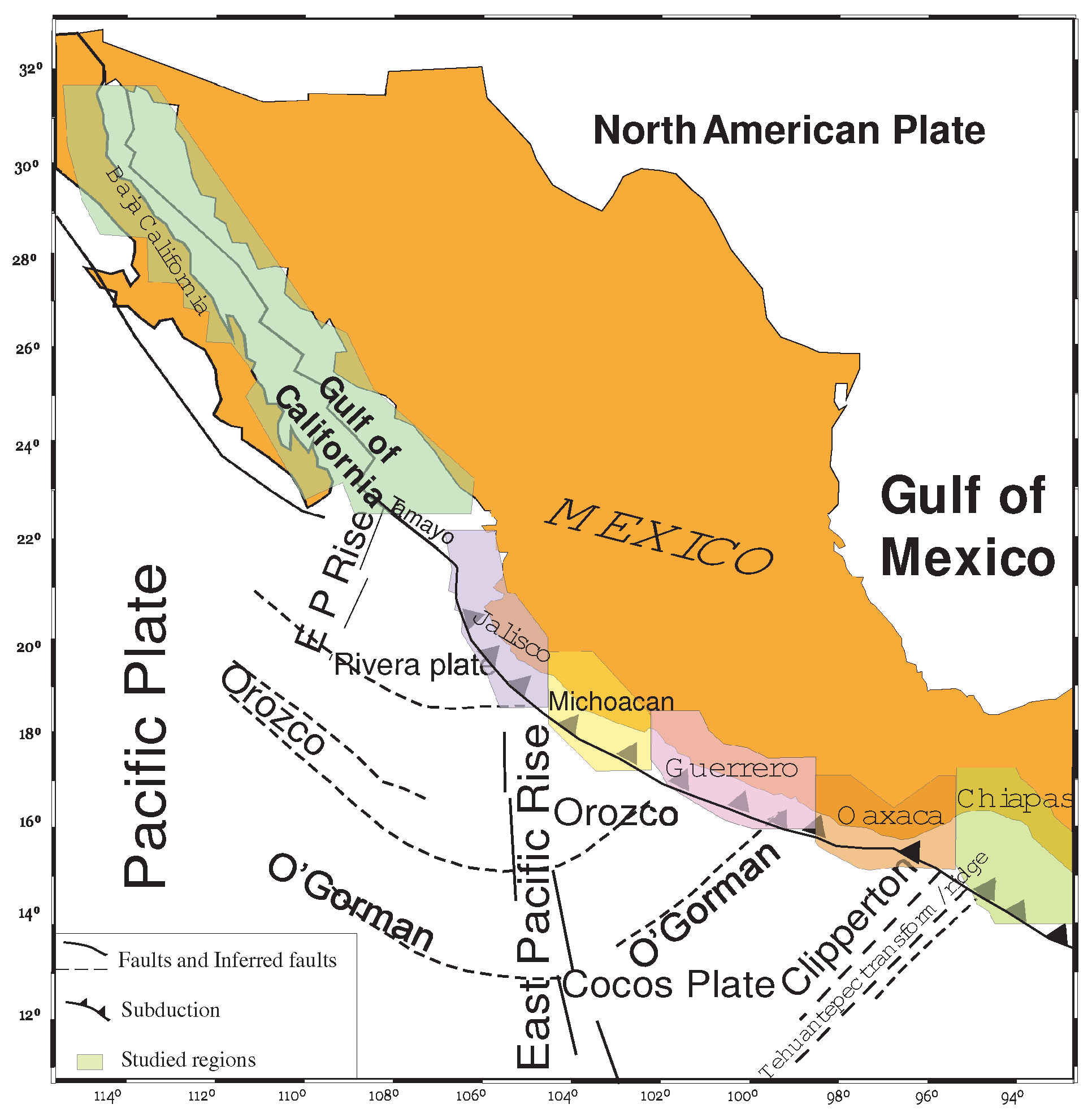
The energy distribution function of earthquakes is obtained by substituting relation (8) into Equation (7) to yield [12]

$$p\left(E\right)dE=\frac{C_1{E}^{-1/3}dE}{{\left[1+C_2{E}^{2/3}\right]}^{1/(q-1)}},$$

(9)

where $C_1=2/\left(3{\alpha }^{2/3}\right)$ and $C_2=(q-1)/\left[(2-q){\alpha }^{2/3}\right]$. If $n\left(E\right)$ is the number of earthquakes of energy E and $N_t$ denotes the total number of earthquakes, then the probability of the energy is given by the expression $p\left(E\right)=n\left(E\right)/N_t$. Integration of the energy distribution function (9) from $E_{\mathrm{th}}$ to ∞, where $E_{\mathrm{th}}$ is a threshold energy, and using the relation $m=(1/3)lnE$ [39], where m is the earthquake magnitude, yields the cumulative number of earthquakes with magnitudes greater than a threshold value M, namely, $N_{>M}$, in a seismic region [12]:

$$ln{N}_{>M}=ln{N}_t+ln{\left[1-\left(\frac{q-1}{q-2}\right)\frac{{10}^{2M}}{{\alpha }^{2/3}}\right]}^{(q-2)/(q-1)}.$$

(10)

It must be emphasized that the q-index in Equation (10) is related to the earthquake energy distribution (9). Equation (10) incorporates the principles of non-extensive thermodynamics into the distribution of earthquakes as a function of the magnitude and represents a widely used form of the non-extensive modification of the GR law based on Tsallis entropy. If the same algebraic steps leading to Equation (10) are applied based on the classical BG statistics, the following frequency–magnitude is obtained

$$ln{N}_{>M}=A-{10}^{2M}B,$$

(11)

where A and B are data-adjustable parameters. In passing, we note that Equation (10) reduces to Equation (11) when $q\to 1$ (see Appendix C). In general, Equation (11) works correctly only for low seismicity, i.e., for earthquakes with magnitudes $\lesssim M_{\mathrm{c}}$. In Equation (10), the entropic index q takes values in the interval $[1,2]$, while the constant $\alpha$ can vary between ${10}^{-3}$ and ${10}^{11}$. In particular, the q-index is a measure of the length scale of the spatial interactions. A q-value close to unity is indicative of short-range correlations, while higher values are indicative of long-term interactions, and therefore, more instability. In terms of the fragment–asperity interaction model, high values of q are indicative of fault planes in relative motion and, as a result, of the fact that more seismic events are expected [11].

3. Tectonic Setting

As was pointed out before, Mexico is a seismically active region because its west coastline lies on the eastern rim of the Ring of Fire, where several tectonic plates interact. It is well documented that its seismicity is caused by different tectonic regimes, namely, the dispersion zone in the Gulf of California and two subduction processes caused by the Rivera and Cocos Plates, which are subducting beneath the continental edge of the North American Plate. Several studies have been conducted to investigate the Cocos subduction zone, motivated primarily by the dangerous earthquakes that took place there. In particular, complete studies of the Mexican subduction regions that take into account the geometry of the Rivera and Cocos Plates can be found in Refs. [25,28,30].

The Gulf of California Rift is part of the East Pacific Rise. It is a spreading boundary where two tectonic plates are moving away from each other, leading to the formation of a new oceanic crust. It is also the southern terminus of the San Andreas Fault [40]. The abundance of neotectonic problems posed by the juxtaposition of the tectonic plates in Mexico has forced the use of the Global Positioning System (GPS) technology, which was initially limited to some areas of the Pacific coast and mainly to the Baja California region. A number of authors [41,42,43,44,45,46] have investigated these neotectonic problems, finding that the city of La Paz (Capital of Baja California) is moving southeast relative to the Pacific Plate, which is consistent with the hypothesis that the Peninsula of Baja California is not completely attached to the Pacific Plate. The Baja California Seismic Network (NARS-Baja) stations provided a new dataset to determine some lithospheric properties on a regional scale. These seismic catalogs have greatly assisted tectonic studies in the Gulf of California by locating active structures [47].

The Rivera microplate is located just south of the Peninsula of Baja California. It is bounded to the northwest by the East Pacific Rise, to the southwest by the Rivera Transform Fault, to the southeast by a deformation zone, and to the northeast by the Middle America Trench and another deformation zone, where an important geological feature is found, the Rivera Triple Junction, located at the southern end of the Peninsula of Baja California. It is also described as an R-R-R (ridge–ridge–ridge)-type junction, which lies along the segment of the East Pacific Rise, which runs between the Rivera Transform Fault and the Tamayo Fault, although the third axis of the junction is not clearly defined. Suhardja et al. [48] investigated the subduction of the Rivera and Cocos Plates in southwestern Mexico. Their project, MARS (Mapping the Rivera Subduction Zone), consisted of an array of 50 temporary seismometer stations to perform the receiver function analysis. They found that the crustal thickness varies from 20 km near the coast to 42 km in the continental interior. The Rivera Plate has a dip steeper than the Cocos Plate along the coast and it is about 10 km deeper than was previously estimated by Pardo and Suarez [28]. The number of seismic imaging studies of the Mexican subduction zone has increased considerably in this century, unraveling the complex interaction of the tectonic plates. The southern part of the Mexican Volcanic Belt shows velocities around 0–4 mm yr⁻¹ for its present slip. The high-resolution image obtained by the analysis of the MASE (MesoAmerican Subduction Experiment) seismic data showed that the flat slap is very shallow and stays this way nearly horizontal for 250 km, lying flat against the continental crust. The Mexican subduction zone could not only be affected by unusual thicknesses of the incoming oceanic crust, but also by atypical forearc dynamics.

Kazachkina et al. [45] revealed an active shear zone parallel to the Middle America Trench about 650 km long by using continuous GPS records gathered over a time span of more than a decade in the Guerrero region. This left-lateral shear zone delimits a wide forearc sliver that moves over the subducting Cocos Plate at a rate of 3–6 mm yr⁻¹ with respect to the North American Plate [49]. The long-term effects of this sliver on the subduction dynamics for the unusually shallow Mexican flat slab are still a matter of research. The subduction in southern Mexico can be approximated by a subhorizontal slab (the flat slab) bounded at its edge by the steep subduction geometry of the Cocos Plate beneath the Caribbean Plate to the east and by the Rivera Plate beneath the North American lithosphere to the west. Subduction zones are prone to generate strong earthquakes, as is indeed the case in the Oaxaca and Chiapas regions, which have experienced a few strong events over the years of magnitude greater than M8 [19].

On the other hand, Carciumaru et al. [50] have recently identified two slab tearings, one on the Michoacán–Guerrero border and the other in Oaxaca, near the Tehuantepec Fracture Transform/Ridge. The slab tearing on the Michoacán–Guerrero border constitutes an important change in the subducting slab, while the one near the Tehuantepec Fracture Transform/Ridge marks the inflection point of the trench that slightly changes its trend to the southeast of the Cocos Plate convergence rate. However, the slides on both sides of the Tehuantepec Ridge are different (i.e., 6.43 and 7.2 cm yr⁻¹) [51]. Figure 1 shows a tectonic map of Mexico, where the seismic zones along the west Mexican coastline are highlighted with different colors. The location of the East Pacific Rise is marked by broken solid lines and fracture zones are marked by dashed lines. The subduction regime of Oaxaca and Chiapas is dominated by the Tehuantepec Transform/Ridge. The enhanced seismic tomography performed by Calò [51] has shown that this fracture is responsible for the vertical propagating tear that controls the magmatism of the El Chichón volcano [52,53] and has also identified the presence of lateral bending, windows, tears, and incipient fragmentation in the first 200–250 km of the subducted plate.

As shown in Figure 1, in terms of its seismicity the southern part of Mexico can be divided into five main regions [19]: (1) the Jalisco region to the west, where the Rivera Plate subducts at a steep angle; (2) the Michoacán region, where the dip angle of the Cocos Plate decreases gradually in the southeast direction; (3) the Guerrero zone, bounded by the Orozco and O’Gorman Fractures; (4) the northern Oaxaca region, where the subducted slab is nearly subhorizontal and underplates the upper continental plate for ∼250 km; and (5) the southern Oaxaca and Chiapas regions, bounded by the Clipperton Fracture, while the Tehuantepec Ridge, which is a linear undersea ridge, extends from the eastern end of the Clipperton Fracture into the Chiapas region, where the dip of the subduction increases gradually to a steeper subduction of the Central America Trench. In particular, the Tehuantepec Ridge is one prominent structure of the Cocos Plate and its tectonic evolution has not been investigated in depth yet [54]. The seismicity in the northern part of the Mexican coastline is characterized by active structures in the Gulf of California, which extends about 1300 km from the fast-spreading mid-ocean ridge system of the East Pacific Rise to the San Andreas Transform Fault zone in southern California. In particular, crustal deformation is active over the full length of the gulf, ranging from classic ridge-transform structures in the south to diffuse deformation in the north [47,55].

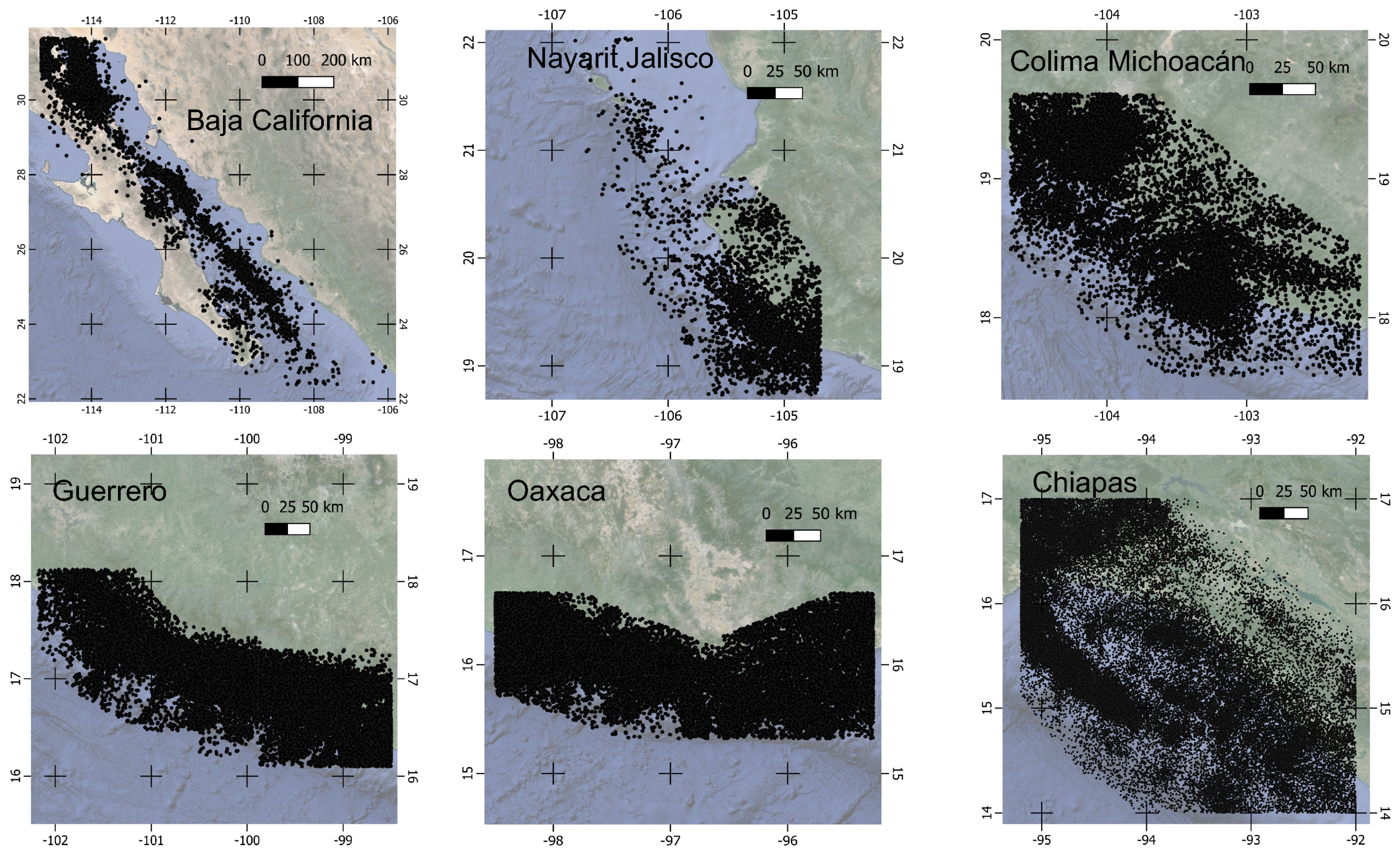
4. Earthquake Data and Analysis Procedure

In this work, we use the corrected Mexican seismic catalog provided by the National Seismic Service (http://www.ssn.unam.mx, accessed on 20 April 2024).The investigated period spans from 1 January 2000 to 13 October 2023. The spatial distribution of earthquakes in each of the six studied regions in Figure 1 is displayed in Figure 2. The symbols (filled dots) in each region mark the actual locations of the epicenters. The spatial distribution of earthquake epicenters over each region was calculated using data from the corrected Mexican seismic catalog with the aid of the geographic information system (QGIS) software 3.34.6 (https://www.qgis.org/es/site/, accessed on 20 April 2024). Darkest zones with the highest concentration of symbols (epicenters) are indicative of sustained seismic activity. Starting from the second column,

Table 1. Seismic activity along the west coastline of Mexico.

Region	${\mathit{M}}_{\mathbf{min}}$	${\mathit{M}}_{\mathbf{max}}$	Number of Earthquakes	${\mathit{M}}_{\mathbf{c}}$
Baja California	1.4	6.8	9579	3.70
Nayarit–Jalisco	2.3	5.9	3774	3.30
Colima–Michoacán	1.9	7.7	20,229	3.45
Guerrero	1.9	7.4	33,080	3.65
Oaxaca	1.2	7.5	59,803	3.46
Chiapas	1.6	8.2	67,008	3.76

lists the minimum magnitude, $M_{\min }$, the maximum magnitude, $M_{\max }$, the number of recorded events, and the magnitude of completeness, $M_{\mathrm{c}}$, for each investigated region.

The Oaxaca and Chiapas regions display the largest number of earthquakes, while the Jalisco region has the lowest activity. The minimum magnitude varies from region to region in the interval between 1.2 (Oaxaca) and 2.3 (Jalisco). During the period investigated, the strongest earthquakes occurred in Chiapas, with a magnitude of 8.2, and Michoacán, with a magnitude of 7.7. With the exception of Baja California and Jalisco, all regions have experienced earthquakes with magnitudes $M>7$. The magnitudes of completeness in the last column of Table 1 were calculated from the recorded data using the method of maximum likelihood estimation (MLE).

The data are first analyzed in terms of the classical GR law:

$$log{N}_{>M}=a-bM,$$

(12)

where the parameter a quantifies the seismicity rate of a region and b is the slope of the cumulative distribution, which is close to unity for tectonic earthquakes. This log-linear dependence of the number of earthquakes of magnitude greater than M on the value of M fails for low and large magnitudes, where the dependence deviates from linear. A non-extensive description of the catalog data is here obtained using the normalized cumulative distribution, $N_{>M}/N_t$, given by Equation (10). For each region the value of the non-extensive parameters q and $\alpha$ are estimated by fitting the observed distribution with the non-extensive model of Equation (10). This was achieved by means of a minimization procedure using two different algorithms, namely, the differential genetic evolution (DGE) [56] and the Broyden–Fletcher–Goldfarb–Shanno (BFGS) optimization algorithm [57]. DGE is an optimization algorithm that works iteratively improving a candidate solution with regard to a given measure of quality. Unlike gradient descent and Newton methods, it does not use the gradient of the problem being optimized, and therefore, the method is computationally efficient. In contrast, the BFGS algorithm pertains to the family of quasi-Newton methods. This method has become popular for parameter estimation in machine learning and typically uses a limited amount of computer memory. Here, both optimization methods are used for the first time to fit non-extensive cumulative distributions of earthquakes to seismic catalog data.

5. Results

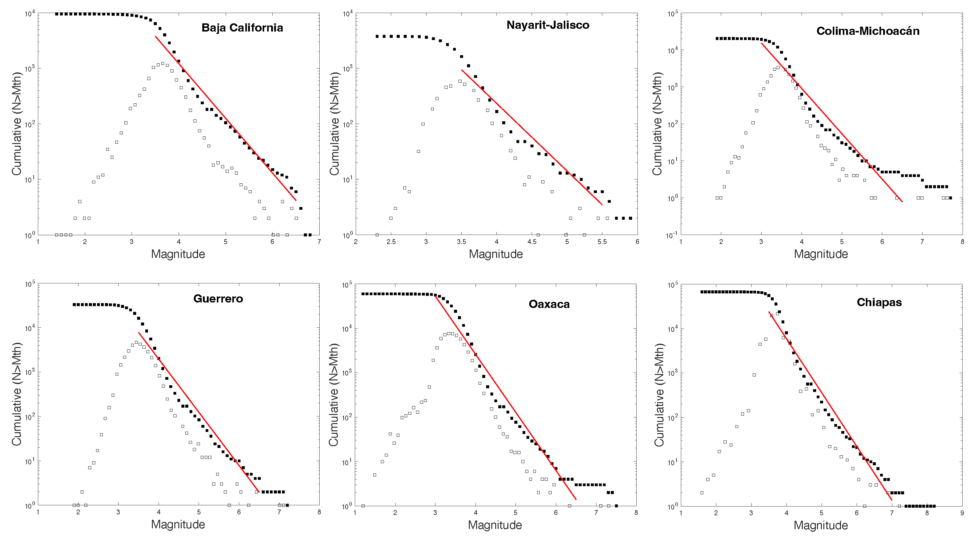
5.1. The Gutenberg–Richter (GR) Law

The classical GR law (12) has played an important historical role in seismology because it was long used to characterize local seismicity and estimate magnitudes of completeness. However, its graphical representations for different catalogs show that it cannot reproduce the correct dependence for the smallest magnitudes. It also fails to describe the energy distribution for large magnitudes. In other words, the linear fitting of the GR law cannot account for magnitudes lower than $M_{\mathrm{c}}$ and, in general, is not representative of extreme seismic events. Therefore, when plotting the frequency–magnitude relation its reliability is limited to a range of intermediate magnitudes for which the linear fitting matches the observed data.

Figure 3 depicts the GR law for the six regions examined. In each plot, the red line shows how well the linear fitting of the GR law reproduces the catalog data. In all cases, the GR relation is satisfied for magnitudes $>M_{\mathrm{c}}$ and smaller than about 5. The worst case corresponds to the Oaxaca catalog where magnitudes larger than ∼4 do not fit the GR law. To the left of the cumulative distribution the frequency distribution of earthquakes as a function of the magnitude is also depicted for each investigated region (empty squares). In all cases, the distributions peak close to the magnitude of completeness, implying that in all regions earthquakes with magnitudes $3.3\lesssim M\lesssim 3.76$ are much more frequent, while stronger events are towards the right tail of the distribution. The values of the parameters a and b in Equation (12) are sensitive to whether or not the cumulative distribution is normalized to the number of earthquakes (see Equations (13)–(15) below).

Table 2. GR-law parameters a and b for the six regions investigated.

Region	a for ${\mathit{N}}_{>\mathit{M}}$ (Non-Normalized)	b for ${\mathit{N}}_{>\mathit{M}}$ (Non-Normalized)	$\tilde{\mathit{a}}$ for ${\mathit{N}}_{>\mathit{M}}/{\mathit{N}}_{\mathit{t}}$ (Normalized)	$\tilde{\mathit{b}}$ for ${\mathit{N}}_{>\mathit{M}}/{\mathit{N}}_{\mathit{t}}$ (Normalized)
Baja California	$7.010\pm 0.05$	$-0.991\pm 0.01$	$3.236\pm 0.40$	$-1.031\pm 0.02$
Nayarit–Jalisco	$6.814\pm 0.18$	$-1.135\pm 0.04$	$4.435\pm 0.20$	$-1.416\pm 0.03$
Colima–Michoacán	$7.518\pm 0.48$	$-1.148\pm 0.10$	$5.480\pm 0.49$	$-1.743\pm 0.01$
Guerrero	$8.280\pm 0.12$	$-1.243\pm 0.02$	$4.132\pm 0.10$	$-1.345\pm 0.02$
Oaxaca	$8.634\pm 0.03$	$-1.327\pm 0.01$	$4.925\pm 0.30$	$-1.574\pm 0.01$
Chiapas	$9.266\pm 0.35$	$-1.359\pm 0.08$	$4.006\pm 0.69$	$-1.273\pm 0.03$

displays the values of a and b for both cases along with their intervals of uncertainty.

When the GR law is not normalized with respect to the total number of earthquakes per region, the b-values are closer to unity compared to the $\tilde{b}$-values for the normalized GR law. In this latter case, the normalized GR law becomes

$$log\frac{N_{>M}}{N_t}=\tilde{a}-\tilde{b}M,$$

(13)

where the parameters $\tilde{a}$ and $\tilde{b}$ are related to those in Equation (12) by the following relations:

$$\begin{array}{ccc}\hfill \tilde{a}& =& a-\frac{1}{2}log{N}_t,\hfill \end{array}$$

(14)

$$\begin{array}{ccc}\hfill \tilde{b}& =& b+\frac{1}{2}\frac{log{N}_t}{M}.\hfill \end{array}$$

(15)

In general, values of the slope close to unity mean that these regions are all seismically active. The normalized $\tilde{a}$-values are all greater than 4, with the exception of the Baja California region where $\tilde{a}\approx 3.24$. When $N_{>M}$ is not normalized the a-values are higher than the normalized ones by factors of about 2. If the analysis of seismicity is performed in terms of normalized cumulative distributions, the set of parameters ( $\tilde{a}$, $\tilde{b}$) is preferred. Otherwise, the set (a, b) is preferred.

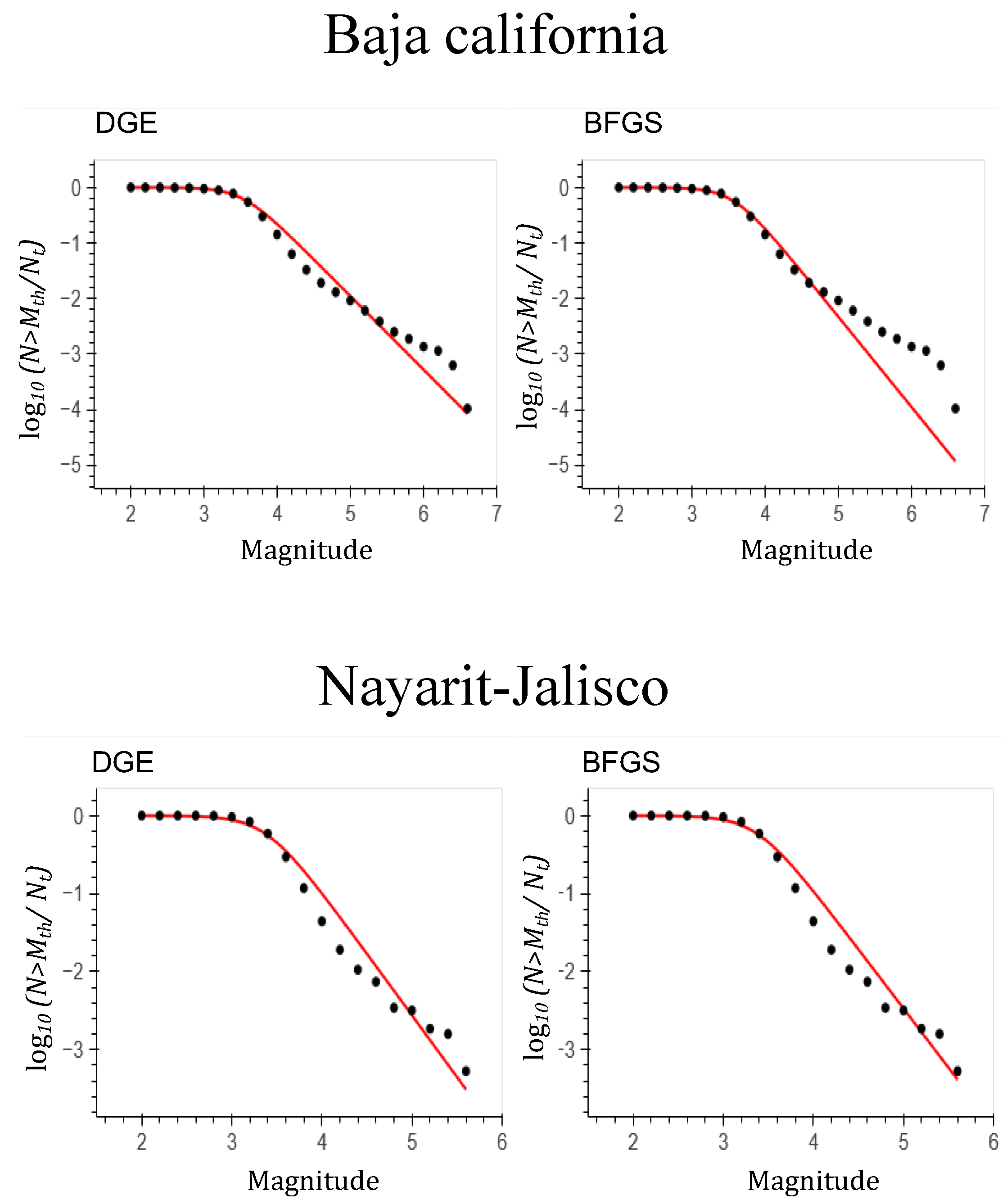
5.2. Non-Extensive Analysis

For each region the value of the non-extensive parameters are estimated by fitting the observed distribution with the non-extensive model of Equation (10). The best fitting is obtained when the square-2 norm attains either a minimum value or reaches a fixed value by using two consecutive procedures. First, the Monte Carlo method was applied to evaluate Equation (10) in the intervals reported by Valverde-Esparza et al. [19], i.e., $1<q<2$ and $\alpha \in ({10}^{-3},{10}^{11})$. The initial value of the entropic index, $q_0$, is set equal to 1.5, while ${\alpha }_0$ is chosen randomly from a million values between ${10}^{-3}$ and ${10}^{11}$ so that optimal intervals around these initial values are defined to be $q_0\pm 0.2$ and ${\alpha }_0\pm {10}^{-3}$, and a couple of initial values ( $q_0$, ${\alpha }_0$) are then proposed. The second procedure consists of using the selected couple of values ( $q_0$, ${\alpha }_0$) as the initial guess for the DGE and BFGS algorithms to obtain the values of q and $\alpha$. A common drawback of these methodologies is that the optimal initial values $q_0$ and ${\alpha }_0$ leading to a minimum error are unknown, and therefore, they must be varied by trial and error until a satisfactory error level is found. The second, third, fourth, and fifth columns of

Table 3. Non-extensive Tsallis entropic parameters for the six regions investigated.

Region	${\mathit{q}}_0$ (DGE)	${\mathit{\alpha }}_0$ (DGE)	q (DGE)	$\mathit{\alpha }$ (DGE)	q (BFGS)	$\mathit{\alpha }$ (BFGS)
Baja California	1.50	6.87 (10)	1.60	6.878 (10)	1.55	6.878 (10)
Nayarit–Jalisco	1.56	1.97 (10)	1.56	1.978 (10)	1.57	1.978 (10)
Colima–Michoacán	1.58	1.50 (10)	1.59	1.670 (10)	1.60	1.670 (10)
Guerrero	1.50	8.40 (10)	1.54	5.432 (10)	1.55	5.432 (10)
Oaxaca	1.59	2.70 (10)	1.53	2.746 (10)	1.61	2.746 (10)
Chiapas	1.60	2.13 (11)	1.58	2.134 (11)	1.59	2.134 (11)
Oaxaca (part 1)	1.60	8.90 (9)	1.50	8.913 (9)	1.61	8.913 (9)
Oaxaca (part 2)	1.60	8.00 (9)	1.59	8.000 (8)	1.61	8.913 (9)

list the optimal initial values of $q_0$ and ${\alpha }_0$ for which a minimum error along with stable values of q and $\alpha$ were obtained.

Figure 4 shows the computed cumulative distribution of events for the Baja California and Jalisco regions. In particular, the seismicity of the Baja California region is caused by the dispersion zone, which is a continuation of the San Andreas Fault, and is here analyzed for the first time using the Sotolongo-Costa and Posadas [11,12] non-extensive model of rock fragmentation. The solid curves represent the best-fit model functions. The plots on the left side correspond to the best fit to the empirical data as obtained with the DGE method, while those on the right side are the best fits obtained using the BFGS method. The fourth and fifth columns of Table 3 list the values of q and $\alpha$ from the DGE fitting, while those in the sixth and seventh columns list those from the BFGS fitting. Both methods yield the same values of $\alpha$ for both regions, i.e., $\alpha \approx 6.88\times {10}^{10}$ (Baja California) and $\alpha \approx 1.98\times {10}^{10}$ (Jalisco). Conversely, the q-values are more sensitive to the choice of the optimization method. For example, the DGE method yields $q=1.60$ (Baja California) and 1.56 (Jalisco), while the BFGS method produces slightly different values (i.e., $q=1.55$ for the Baja California region and $q=1.57$ for the Jalisco region).

As an example, the error calculated as the difference between the computed and cumulative value as a function of $q_0$ and ${\alpha }_0$ is displayed in Figure 5 for the case of Baja California when the iteration was performed using the BFGS method. This plot exemplifies the procedure followed to obtain the minimum error. Similar plots were obtained for all other regions. The minimum error is achieved when $q_0=1.50$ and ${\alpha }_0=6.87\times {10}^{10}$. For this case the value of the error is stable for ${\alpha }_0>{10}^{10}$. On the other hand, Figure 6 shows the best fits obtained for the Michoacán and Guerrero regions using the DGE and BFGS methods. The DGE analysis yields q-values of 1.59 (Michoacán) and 1.54 (Guerrero), while the BFGS analysis results in slightly higher values, i.e., 1.60 (Michoacán) and 1.55 (Guerrero). These values are comparable to the ones obtained for the Baja California and Jalisco regions, which according to Table 1 have a much lower incidence of events compared to Michoacán and Guerrero. Therefore, this suggests that all these four regions are equally unstable, independently of the historical record of earthquakes.

Finally, Figure 7 shows the normalized cumulative distribution function for the Oaxaca and Chiapas regions. Although the Chiapas region is known to be a highly active seismic region (see Figure 2), its seismicity has not been previously studied using a non-extensive approach to determine the value of the q-entropic index. These two regions share the largest numbers of recorded earthquakes (see Table 1). However, their estimated entropic indices were $q=1.53$ (Oaxaca) and $q=1.58$ (Chiapas) when the analysis was performed using the DGE method. Again, a much higher value of $q(=1.61)$ was obtained for the Oaxaca region with the BFGS method, while only a slightly higher value ($q=1.59$) was estimated for the Chiapas region. The results show that the distribution of recorded events can be well described by the generalized GR law given by Equation (10), especially for low magnitudes with q-entropic indices between 1.53 and 1.60 when using the DGE method and between 1.55 and 1.61 when using the BFGS method. A comparison between both methods (Figure 4, Figure 6 and Figure 7) shows that BFGS performs slightly better than DGE. However, for the Baja California region DGE appears to perform better than BFGS since the latter deviates substantially from the observed data for $M>5$ compared to the former method.

From the analysis of the frequency–magnitude distributions of all six regions, it is clear that the fragment–asperity model describes the seismic behavior of the western Mexican coastline fairly well, perhaps except at the largest magnitudes towards the lower end of the distributions. This feature is more prominent for the Baja California region (Figure 4). In other words, the q-entropic index describes the complexity of the tectonic system along the Pacific coast of Mexico with values between 1.50 and 1.60, supporting sub-additivity of the frequency–magnitude distribution of earthquakes. A previous non-extensive analysis of seismicity in Mexico, spanning the period from 1988 to 2000, yielded values of the entropic index in the interval $1.663\lesssim q\lesssim 1.702$ for the southern Mexican seismicity, comprising the regions of Jalisco, Michoacán, Guerrero, and Oaxaca [19]. These values are slightly larger than those reported by the present analysis. A possible cause of this difference can be attributed to the use of improved seismic recording equipment during the last decade, which is more sensitive to the detection of low-magnitude events than older instrumentation, and to the increasing number of seismic stations. Increasing the number of recorded earthquakes of low magnitude will contribute to lowering the estimated values of the q-entropic index.

A close inspection of the two upper plots of Figure 7 for the Oaxaca region reveals that the observed data for magnitudes $>M_c$ are characterized by at least three different slopes for low ($M_c\lesssim M\lesssim 4.5$), intermediate ($4.5\lesssim M\lesssim 6.4$), and large ($M\gtrsim 6.5$) magnitudes. This means that it is not possible to fit a unique curve for the whole range of magnitudes in the Oaxaca region, as was first reported by Valverde-Esparza et al. [19]. In particular, the crossover at a magnitude of about 4.5 is indicative of the Oaxaca region being characterized by two different subduction processes since this region comprises the earthquakes that took place in the zones between the Tehuantepec Transform/Ridge and the Clipperton Fracture (Oaxaca, part 2) and the zones between the Clipperton and O’Gorman Fractures (Oaxaca, part 1). Figure 8 shows the normalized cumulative distribution of events for both sub-regions as obtained with the DGE (left plots) and BFGS (right plots) optimization methods. These fits provided values of $q=1.50$ with the DGE method and $q=1.61$ with the BFGS method for Oaxaca, part 1, and values of $q=1.59$ with the DGE method and $q=1.61$ with the BFGS method for Oaxaca, part 2 (see Table 3). It is clear that the q-values for the Oaxaca, part 2 sub-region are closer to those for the Chiapas region, while those derived for the Oaxaca, part 1 sub-region are closer to those corresponding to the Guerrero region. This latter statement is at least valid for the DGE values. We note that the same is not necessarily true for the BFGS values, where $q=1.61$ for both the complete and the two sections of the Oaxaca catalog. An important novel point of the present analysis is that it includes earthquake data pertaining to the last twenty years, which were recorded by the new seismic monitoring network of broadband sensors disseminated along the full west coastline of Mexico. Therefore, the new estimated values of q for all six regions studied provide a more accurate and reliable measure of the seismic hazard present in all of them. These improved values of q takes into account a much larger number of low-magnitude events than was possible before with the use of old instrumentation, thereby explaining the slightly lower q-values reported for all sub-regions compared to those previously estimated by Valverde-Esparza et al. [19].

6. Conclusions

A seismic analysis of magnitude catalogs from 2000 to 2023 of the Mexican South Pacific was performed by means of the NESM approach based on the Tsallis formalism. We analyzed six regions along the west coastline of Mexico, namely, Baja California, Nayarit-,Jalisco, Colima-,Michoacán, Guerrero, Oaxaca and Chiapas, which are characterized by different tectonic regimes. The seismicity of the Gulf of California (Cortes Sea) is caused by the dispersion zone which is a continuation of the San Andreas Fault. In contrast, the seismic activity in the Nayarit–Jalisco and Colima–Michoacan regions is mainly due to the subduction process of the Rivera Plate, while the seismicity of the Guerrero, Oaxaca, and Chiapas regions is mainly caused by the subduction of the Cocos Plate. In both cases, the plates are subducting beneath the continental edge of the North American Plate. The relevant conclusions from this analysis are summarized as follows:

• According to the Gutenberg–Richter (GR) law all six regions have magnitudes of completeness in the range between 3.30 and 3.76, implying that along the Pacific coast of Mexico earthquakes with magnitudes in this range are more frequent.
• The Oaxaca and Chiapas regions share the largest number of earthquakes, while the regions of Jalisco and Baja California show the lowest activity.
• The GR-law parameters a and b are sensitive to whether or not the cumulative distribution is normalized to the number of earthquakes. In particular, the non-normalized b-parameter is close to unity for all six regions, meaning that they are all seismically active tectonic zones.
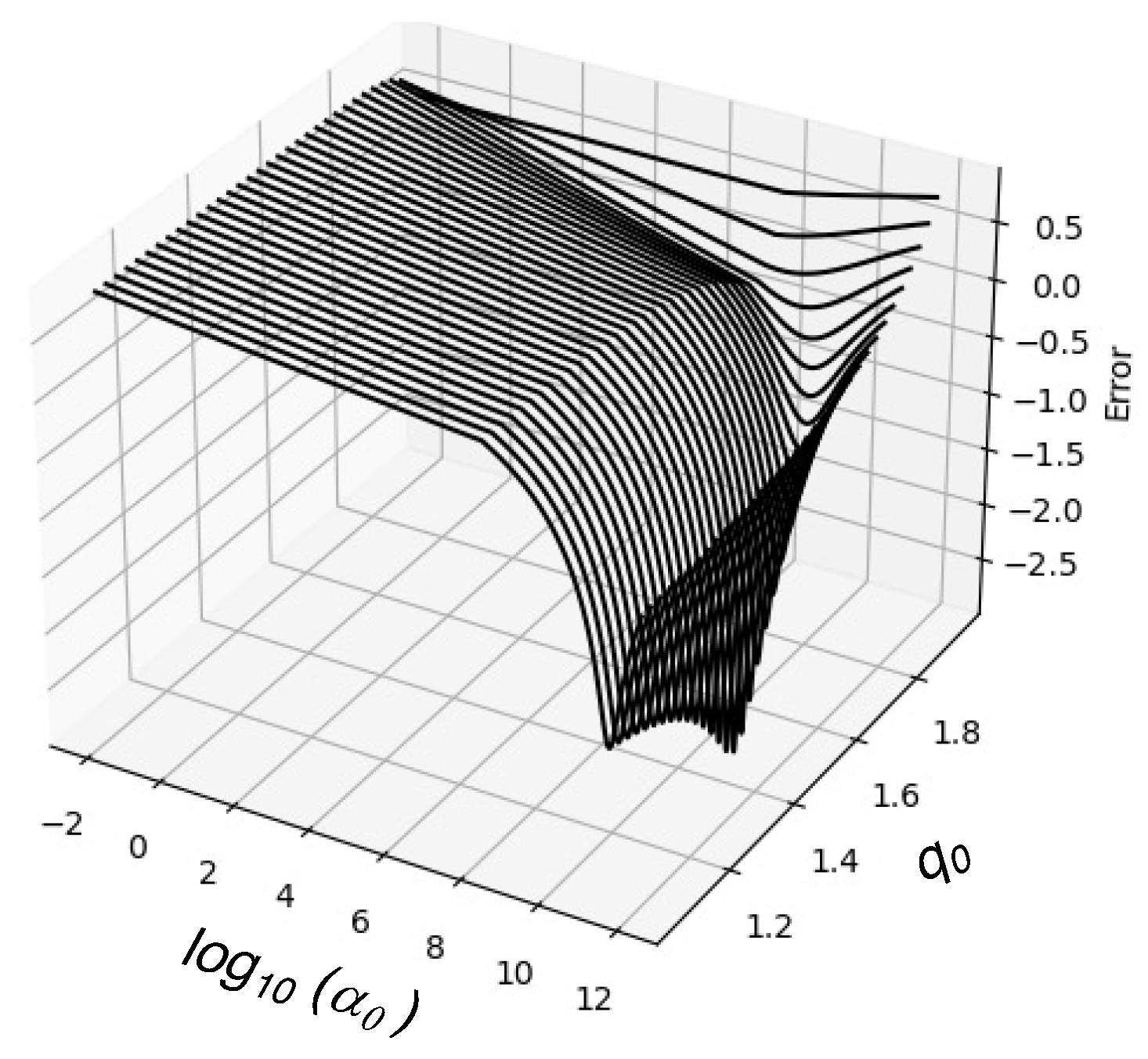
• A non-extensive model fitting with the observed distributions of earthquakes was obtained using two different optimization methods, namely, the differential genetic evolution (DGE) and the Broyden–Fletcher–Goldfarb–Shanno (BFGS) algorithm. The entropic index, q, and the parameter $\alpha$ derived from the two methods both show little difference; for q it is less than about 0.05 for all cases studied.
• The $\alpha$-values ranged between a low value of $1.670\times {10}^{10}$ (for the Colima–Michoacán region) and a maximum value of $2.134\times {10}^{11}$ (for the Chiapas region).
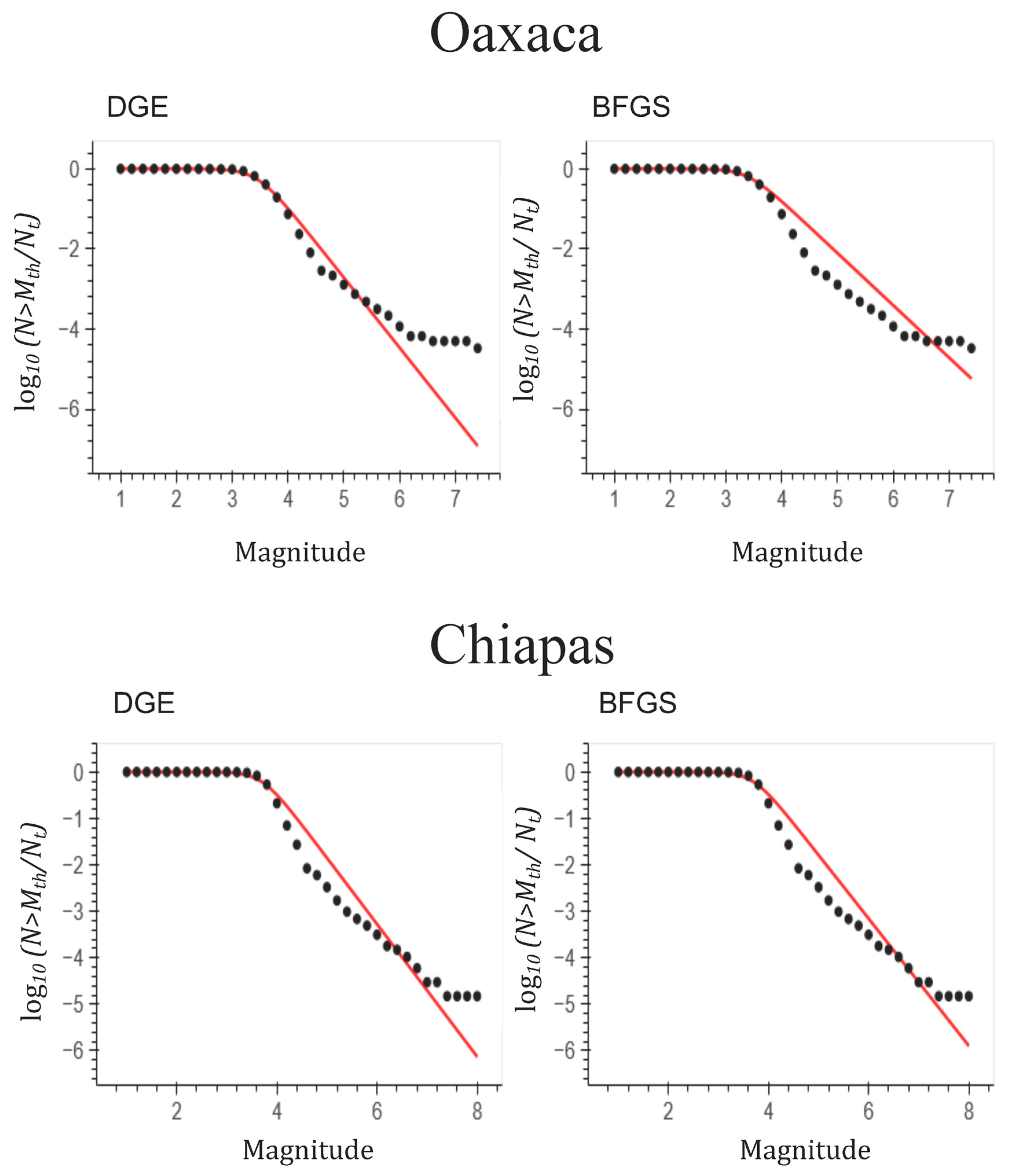
• The whole range of magnitudes recorded for the Oaxaca region cannot be fitted by a unique curve since for magnitudes close to 5 the slope of the normalized cumulative magnitude distribution changes, implying a clear crossover for this region. When both sub-regions are analyzed separately, both optimization methods predict lower values of $\alpha$.
• A value of q close to unity is indicative of short-range correlations, while higher values are indicative of long-term interactions, and therefore, of more instability. In terms of the fragment–asperity interaction model, values of $q>1$ are indicative of fault planes in relative motion, implying that more seismic events are expected. All six regions display values of q greater than 1.52, suggesting instability and long-term correlations. In particular, the regions of Baja California, Colima–Michoacán and Chiapas had the largest values of q, between 1.58 and 1.60.
• In comparison with a previous similar analysis spanning the period from 1988 to 2010, updated estimates of q were obtained to be from 1.70 to 1.56–1.57 for Jalisco, from 1.68 to 1.59–1.60 for Michoacán, from 1.64 to 1.54–1.55 for Guerrero, and from 1.66 to 1.53–1.61 for Oaxaca. The predicted lower values of q are a consequence of the use of the new monitoring network of broadband sensors distributed along the entire Pacific coast of Mexico, which are more sensitive to the detection of low-magnitude earthquakes.

References

1. Tsallis, C. What should a statistical mechanics satisfy to reflect nature? Phys. D 2004, 193, 3–34. [Google Scholar] [CrossRef]
2. Tsallis, C. Nonadditive entropy and nonextensive statistical mechanics—An overview after 20 years. Braz. J. Phys. 2009, 39, 337–356. [Google Scholar] [CrossRef]
3. Tsallis, C.; Tirnakli, U. Nonadditive entropy and nonextensive statistical mechanics—Some central concepts and recent applications. J. Phys. Conf. Ser. 2010, 201, 012001. [Google Scholar] [CrossRef]
4. Tsallis, C. Possible generalization of Boltzmann-Gibbs statistics. J. Stat. Phys. 1988, 52, 479–487. [Google Scholar] [CrossRef]
5. Abe, S.; Okamoto, Y. Nonextensive Statistical Mechanics and Its Applications; Springer: Heidelberg, Germany, 2001. [Google Scholar]
6. Tsallis, C. Introduction to Nonextensive Statistical Mechanics: Approaching a Complex World; Springer: Berlin, Germany, 2009. [Google Scholar]
7. Tsallis, C. The nonadditive entropy Sq and its applications in physics and elsewhere: Some remarks. Entropy 2011, 13, 1765–1804. [Google Scholar] [CrossRef]
8. Abe, S.; Suzuki, N. Law for the distance between successive earthquakes. J. Geophys. Res. 2003, 108, 2113. [Google Scholar] [CrossRef]
9. Papadakis, G.; Vallianatos, F.; Sammonds, P. Evidence of nonextensive statistical physics behavior of the Hellenic subduction zone sismicity. Tectonophysics 2013, 608, 1037–1048. [Google Scholar] [CrossRef]
10. Vallianatos, F.; Sammonds, P. Evidence of nonextensive statistical physics of the lithospheric instability approaching the 2004 Sumatran-Andaman and 2011 Honshu mega-earthquakes. Tectonophysics 2004, 590, 52–58. [Google Scholar] [CrossRef]
11. Sotolongo-Costa, O.; Posadas, A. Fragment-asperity interaction model for earthquakes. Phys. Rev. Lett. 2004, 13, 1267–1280. [Google Scholar] [CrossRef]
12. Silva, R.; França, G.S.; Vilar, C.S.; Alcaniz, J.S. Nonextensive models for earthquakes. Phys. Rev. E 2006, 73, 026102. [Google Scholar] [CrossRef]
13. Lay, T.; Wallace, T.C. Modern Global Seismology; Academic Press: New York, NY, USA, 1995. [Google Scholar]
14. Telesca, L. Maximum likelihood estimation of the nonextensive parameters of the earthquake cumulative magnitude deistribution. Bull. Seismol. Soc. Am. 2012, 102, 886–891. [Google Scholar] [CrossRef]
15. Darooneh, A.M.; Mehri, A. A nonextensive modification of the Gutenberg-Richter law: q-stretched exponential form. Physical A 2010, 389, 509–514. [Google Scholar] [CrossRef]
16. Telesca, L. Analysis of Italian seismicity by using a nonextensive approach. Tectonophysics 2010, 494, 155–162. [Google Scholar] [CrossRef]
17. Telesca, L. Nonextensive analysis of seismic sequences. Physical A 2010, 389, 1911–1914. [Google Scholar] [CrossRef]
18. Matcharashvili, T.; Chelidze, T.; Javakhishvili, Z.; Jorjiashvili, N.; Fra Paleo, U. Non-extensive statistical analysis of seismicity in the area of Javakheti, Georgia. Comput. Geosci. 2011, 37, 1627–1632. [Google Scholar] [CrossRef]
19. Valverde-Esparza, S.M.; Ramírez-Rojas, A.; Flores-Márquez, E.L.; Telesca, L. Non-extensivity analysis of seismicity within four subduction regions in Mexico. Acta Geophys. 2012, 60, 833–845. [Google Scholar] [CrossRef]
20. Antonopoulos, C.G.; Michas, G.; Vallianatos, F. Evidence of q-exponential statistics in Greek seismicity. Physical A 2014, 409, 71–77. [Google Scholar] [CrossRef]
21. Papadakis, G.; Vallianatos, F.; Sammonds, P. A nonextensive statistical physics analysis of the 1995 Kobe, Japan earthquake. Pure Appl. Geophys. 2015, 172, 1923–1931. [Google Scholar] [CrossRef]
22. Papadakis, G.; Vallianatos, F.; Sammonds, P. Non-extensive statistical physics applied to heat flow and the earthquake frequency-magnitude distribution in Greece. Physical A 2016, 456, 135–144. [Google Scholar] [CrossRef]
23. Papadakis, G.; Vallianatos, F. Non-extensive statistical physics analysis of earthquake magnitude in North Aegean Trough, Greece. Acta Geophys. 2017, 65, 555–563. [Google Scholar] [CrossRef]
24. Ohtake, M.; Matumoto, T.; Latham, G.V. Evaluation of the forecast of the 1978 Oaxaca, Southern Mexico earthquake based on a precursory seismic quiescence. In Earthquake Prediction: An International Review; Simpson, D.W., Richards, P.G., Eds.; American Geophysical Union: Washington, DC, USA, 1981; pp. 53–61. [Google Scholar]
25. Singh, S.K.; Rodriguez, M.; Esteva, L. Statistics of small earthquakes and frequency of occurrence of large earthquakes along the Mexican subduction zone. Bull. Seismol. Soc. Am. 1983, 73, 1779–1796. [Google Scholar]
26. Singh, S.K.; Ponce, L.; Nishenko, S.P. The great Jalisco, Mexico, earthquakes of 1932: Subduction of the Rivera plate. Bull. Seismol. Soc. Am. 1985, 75, 1301–1313. [Google Scholar] [CrossRef]
27. Kostoglodov, V.; Ponce, L. Relationship between subduction and seismicity in the Mexican part of the Middle America Trench. J. Geophys. Res. 1994, 99, 729–742. [Google Scholar] [CrossRef]
28. Pardo, M.; Suarez, G. Shape of the subducted Rivera and Cocos plates in southern Mexico: Seismic and tectonic implications. J. Geophys. Res. 1995, 100, 12357–12373. [Google Scholar] [CrossRef]
29. Zúñiga, F.R.; Wiemer, S. Seismic patterns: Are they always related to natural causes? Pure Appl. Geophys. 1999, 155, 713–726. [Google Scholar] [CrossRef]
30. Iglesias, A.; Singh, S.K.; Lowry, A.R.; Santoyo, M.; Kostoglodov, V.; Larson, K.M.; Franco-Sánchez, S.I. The silent earthquake of 2002 in the Guerrero seismic gap, Mexico (Mw = 7.6): Inversion of slip on the plate interface and some implications. Geof. Int. 2004, 43, 309–317. [Google Scholar] [CrossRef]
31. Song, T.-R.A.; Helmberger, D.V.; Brudzinski, M.R.; Clayton, R.W.; Davis, P.; Pérez-Campos, X.; Singh, S.K. Subducting slab ultra-slow velocity layer coincident with silent earthquakes in southern Mexico. Science 2009, 324, 502–506. [Google Scholar] [CrossRef] [PubMed]
32. Ramírez-Herrera, M.T.; Kostoglodov, V.; Urrutia-Fucugauchi, J. Overview of recent coastal tectonic deformation in the Mexican subduction zone. Pure Appl. Geophys. 2011, 168, 1415–1433. [Google Scholar] [CrossRef]
33. Ramírez-Rojas, A.; Flores-Márquez, E. Order parameter analysis of seismicity of the Mexican Pacific coast. Physical A 2013, 392, 2507–2512. [Google Scholar] [CrossRef]
34. Ramírez-Rojas, A.; Flores-Márquez, E.L.; Sarlis, N.V.; Varotsos, P.A. The complexity measures associated with the fluctuations of the entropy in natural time before the deadly Mexico M8.2 earthquake on 7 September 2017. Entropy 2018, 20, 477. [Google Scholar] [CrossRef]
35. Sarlis, N.V.; Skordas, E.S.; Varotsos, P.A.; Ramírez-Rojas, A.; Flores-Márquez, E.L. Natural time analysis: On the deadly Mexico M8.2 earthquake on 7 September 2017. Physical A 2018, 506, 625–634. [Google Scholar] [CrossRef]
36. Abe, S. Geometry of escort distributions. Phys. Rev. E 2003, 68, 031101. [Google Scholar] [CrossRef] [PubMed]
37. Bercher, J.-F. On escort distributions, q-gaussians and Fisher information. AIP Conf. Proc. 2011, 1305, 208–215. [Google Scholar]
38. Ohara, A.; Matsuzoe, H.; Amari, S.-I. Conformal geometry of escort probability and its applications. Mod. Phys. Lett. B 2012, 26, 1250063. [Google Scholar] [CrossRef]
39. Kanamori, H.; Stewart, G.S. Seismological aspects of the Guatemala earthquake of February 4, 1976. J. Geophys. Res. 1978, 83, 3427–3434. [Google Scholar] [CrossRef]
40. Lewis, J.L.; Day, S.M.; Magistrale, H.; Castro, R.R.; Astiz, L.; Rebollar, C.; Eakins, J.; Vernon, F.L.; Brune, J.N. Crustal thickness of the peninsular ranges and gulf extensional province in the Californias. J. Geophys. Res. 2001, 106, 13599–13611. [Google Scholar] [CrossRef]
41. Hearn, T.M.; Clayton, R.W. Lateral velocity variations in southern California. I. Results for the upper crust from Pg waves. Bull. Seismol. Soc. Am. 1986, 76, 495–509. [Google Scholar] [CrossRef]
42. Humphreys, E.D.; Clayton, R.W. Tomographic image of the southern California mantle. J. Geophys. Res. 1990, 95, 19725–19746. [Google Scholar] [CrossRef]
43. Márquez-Azúa, B.; DeMets, C. Crustal velocity field of Mexico from continuous GPS measurements, 1993 to June 2001: Implications for the neotectonics of Mexico. J. Geophys. Res. 2003, 100, 2450. [Google Scholar] [CrossRef]
44. Clayton, R.W.; Heaton, T.H.; Chandy, M.; Krause, R.A.; Kohler, M.; Bunn, J.; Guy, R.; Olson, M.; Faulkner, M.; Cheng, M.; et al. Community seismic network. Ann. Geophys. 2011, 54, 738–747. [Google Scholar]
45. Kazachkina, E.; Kostoglodov, V.; Cotte, N.; Walpersdorf, A.; Ramírez-Herrera, M.T.; Gaidzik, K.; Husker, A.; Santiago, J.A. Active 650-km long fault system and Xolapa sliver in Southern Mexico. Front. Earth Sci. 2020, 8, 155. [Google Scholar] [CrossRef]
46. Schellart, W.P. Control of subduction zone age and size on flat slab subduction. Front. Earth Sci. 2020, 8, 26. [Google Scholar] [CrossRef]
47. Clayton, R.W.; Trampert, J.; Rebollar, C.; Ritsema, J.; Persaud, P.; Paulssen, H.; Pérez-Campos, X.; van Wettum, A.; Pérez-Vertti, A.; DiLuccio, F. The NARS-Baja seismic array in the Gulf of California rift zone. MARGINS Newslett. 2004, 13, 1–8. [Google Scholar]
48. Suhardja, S.K.; Grand, S.P.; Wilson, D.; Guzman-Speziale, M.; Gomez-Gonzalez, J.M.; Dominguez-Reyes, T.; Ni, J. Crust and subduction zone structure of Southwestern Mexico. J. Geophys. Res. 2003, 120, 1020–1035. [Google Scholar] [CrossRef]
49. Manea, V.C.; Manea, M.; Chen, M.; van Hunen, J.; Konrad-Schmolke, M. Editorial: Unusual subsduction processes. Font. Earth Sci. 2020, 8, 607697. [Google Scholar]
50. Carciumaru, D.; Ortega, R.; Castellanos, J.C.; Huesca-Pérez, E. Crustal characteristics in the subduction zone of Mexico: Implication of the tectonostratigraphic terranes on slab tearing. Seism. Res. Lett. 2020, 91, 1781–1793. [Google Scholar] [CrossRef]
51. Calò, M. Tears, windows, and signature of transform margins on slabs. Images of the Cocos plate fragmentation beneath the Tehuantepec isthmus (Mexioc) using Enhanced Seismic Models. Earth Planet. Sci. Lett. 2021, 560, 116788. [Google Scholar] [CrossRef]
52. de Ignacio, C.; Casteiñeiras, P.; Márquez, A.; Oyarzun, R.; Lillo, J.; López, I. El Chichn Volcano (Chiapas Volcanic Belt, Mexico) transitional Calc-Alkaline to Adakitic-like magmatism: Petrologic and tectonic implications. Int. Geol. Rev. 2003, 45, 1020–1028. [Google Scholar] [CrossRef]
53. Manea, M.; Manea, V.C. On the origin of the El Chichón volcano and subduction of Tehuantepec Ridge: A geodynamical perspective. J. Volcanol. Geotherm. Res. 2008, 175, 459–471. [Google Scholar] [CrossRef]
54. Manea, M.; Manea, V.C.; Ferrari, L.; Kostoglodov, V. Tectonic evolution of the Tehuantepec Ridge. Earth Planet. Sci. Lett. 2005, 238, 64–77. [Google Scholar] [CrossRef]
55. Di Luccio, F.; Persaud, P.; Clayton, R.W. Seismic structure beneath the Gulf of California: A contribution from group velocity measurements. Geophys. J. Int. 2014, 199, 1861–1877. [Google Scholar] [CrossRef]
56. Goldberg, D.E. Genetic Algorithms in Search, Optimization and Machine Learning; Kluwer Academic Publishers: Boston, MA, USA, 1989. [Google Scholar]
57. Fletcher, R. Practical Methods of Optimization; John Wiley & Sons: New York, NY, USA, 1987. [Google Scholar]
Figure 1. Tectonic map of Mexico. The seismic regions along the west coastline of Mexico are highlighted with different colors. The locations of the East Pacific Rise (broken solid lines) and the fracture zones (dashed lines), including the Tehuantepec Ridge, are shown. The pattern brush stroke of filled triangles along the southwestern coast represents the subduction zones, with the triangles pointing in the direction of subduction.
Fractalfract 08 00306 g001
Figure 2. Spatial distribution of recorded earthquakes in the six regions investigated along the west coastline of Mexico. The symbols mark the locations of the earthquake epicenters.
Fractalfract 08 00306 g002
Figure 3. GR law (red line) fitted to the earthquake sub-catalog for each of the six regions investigated (filled squares). For each region the frequency distribution of earthquakes as a function of the magnitude is depicted to the left of the cumulative distribution (empty squares).
Fractalfract 08 00306 g003
Figure 4. Normalized cumulative distribution of earthquakes for the seismicity monitored in the Baja California (upper plots) and Jalisco (lower plots) regions (filled dots). The red solid curves correspond to the fittings based on Equation (10). In each case, the left and right plots depict the fitting as obtained using the DGE and BFGS methods, respectively.
Fractalfract 08 00306 g004
Figure 5. Runs performed by varying the initial entropic parameters q 0 and α 0 to determine the optimal guess leading to the minimum error. The figure corresponds to the case of the Baja California region using the BFGS method.
Fractalfract 08 00306 g005
Figure 6. Normalized cumulative distribution of earthquakes for the seismicity monitored in the Michoacán (upper plots) and Guerrero (lower plots) regions (filled dots). The red solid curves correspond to the fittings based on Equation (10). In each case, the left and right plots depict the fitting as obtained using the DGE and BFGS methods, respectively.
Fractalfract 08 00306 g006
Figure 7. Normalized cumulative distribution of earthquakes for the seismicity monitored in the Oaxaca (upper plots) and Chiapas (lower plots) regions (filled dots). The red solid curves correspond to the fittings based on Equation (10). In each case, the left and right plots depict the fitting as obtained using the DGE and BFGS methods, respectively.
Fractalfract 08 00306 g007
Figure 8. Normalized cumulative distribution of earthquakes for the seismicity monitored in the Oaxaca sub-regions: part 1 (upper plots) and part 2 (lower plots). The filled dots correspond to the monitored catalog data, while the red solid curves correspond to the fittings based on Equation (10). In each case, the left and right plots depict the fitting as obtained using the DGE and BFGS methods, respectively.
Fractalfract 08 00306 g008