Analyzing a Dynamical System with Harmonic Mean Incidence Rate Using Volterra–Lyapunov Matrices and Fractal-Fractional Operators

Abstract

This paper investigates the dynamics of the SIR infectious disease model, with a specific emphasis on utilizing a harmonic mean-type incidence rate. It thoroughly analyzes the model’s equilibrium points, computes the basic reproductive rate, and evaluates the stability of the model at disease-free and endemic equilibrium states, both locally and globally. Additionally, sensitivity analysis is carried out. A sophisticated stability theory, primarily focusing on the characteristics of the Volterra–Lyapunov (V-L) matrices, is developed to examine the overall trajectory of the model globally. In addition to that, we describe the transmission of infectious disease through a mathematical model using fractal-fractional differential operators. We prove the existence and uniqueness of solutions in the SIR model framework with a harmonic mean-type incidence rate by using the Banach contraction approach. Functional analysis is used together with the Ulam–Hyers (UH) stability approach to perform stability analysis. We simulate the numerical results by using a computational scheme with the help of MATLAB. This study advances our knowledge of the dynamics of epidemic dissemination and facilitates the development of disease prevention and mitigation tactics.

1. Introduction

Mathematical modeling is an adaptable technique that is used in many different fields and is an effective tool for comprehending, assessing, and forecasting the dynamics of complicated systems and phenomena. It includes the use of mathematical frameworks like equations, graphical representations, or computational methods to depict processes and systems that exist in everyday life. Mathematical modeling has applications in many different domains, such as environmental science, finance, biological sciences, physical sciences, engineering, and humanities. The first step in this method is to precisely define the issue that needs to be solved and to list all of the important factors and specifications. Next, in order to explain the behavior of the system under investigation, models are created, frequently by oversimplifying presumptions. Parameters are determined through estimation using previously collected information or research findings, whereas the reliability of the system is verified through the comparison of the predicted outcomes with real-life data. An analysis is conducted on mathematical aspects of the model, especially stability or sensitivity, in order to comprehend how it behaves across various scenarios. By employing computational approaches, models are used to forecast the expected growth or reaction of the system to different inputs or situations. The outcomes of mathematical modeling eventually produce significant understandings that guide decision making, stimulate new ideas, and contribute to the advancement of our understanding in various domains.

While the COVID-19 pandemic has declined in many regions, certain countries still face the ongoing threat of the virus, as evidenced by findings from Ref. [1]. The article’s primary finding indicates that 8526 people died as a result of the COVID-19 winter wave that hit Italy from 31 October 2022, to 9 February 2023. The height of the outbreak occurred over the holiday weeks of 16 December 2022, to 5 January 2023. The weekly trends in the wave’s growth and decline were $+7.89\%$ and $-15.85\%$, respectively. The same trajectory predicts less than 4100 deaths during the 2023–2024 wave. The initial information from October to December 2023 supports the prediction. For more intricate insights, we direct readers to [2,3,4].

Another recent study in the field of epidemiology [5] created a model to show how undiagnosed tuberculosis (TB) cases during the COVID-19 pandemic affected subsequent infections with M. tuberculosis. The model illustrates the relationship between low screening coverage, missed TB cases, and increased future infections by analyzing data from Russia (2008–2021). The results in the article highlight the urgent need for mass population screening in order to detect tuberculosis cases at an early stage and successfully manage transmission. Based on the above latest research and forecasts, it is evident that the field of infectious disease requires further refinement in methodologies and approaches to effectively tackle and control future infectious disease threats through intervention strategies. Epidemiological studies frequently concentrate on evaluating the worldwide stability of endemic equilibrium in models of infectious diseases. Research articles such as [6,7,8,9] have made valuable contributions to this research. A number of methods, such as monotone dynamical systems, the geometric method, and Lyapunov functions [10,11,12] have been used to show that equilibrium points are stable. Additional perspectives on stability can be gleaned from articles such as [13,14]. The V-L technique is a mathematical structure utilized to analyze complicated structures like viral infection models. Refs. [15,16] are important in this regard. Mathematical modeling, especially with compartmental models like SIR and SEIR, is common in studying diseases like COVID-19, aiding in prediction and intervention evaluation.

Further insights can be found in Refs. [17,18,19]. The V-L approach, stemming from control theory and nonlinear dynamics, provides insights into system stability and behavior. It analyzes equilibrium stability, parameter effects, and system resilience in an infectious disease. Further research into the V-L approach could enhance understanding of other infectious diseases. In this article, we develop a sophisticated stability theory, primarily focusing on the characteristics of the V-L matrices method.

In the most recent progress in fractional calculus, as described in [20], the authors created a time-fractional COVID-19 model using a fractal-fractional operator. They then tested its validity and stability and ran simulations to learn more about how epidemics spread. In another recent advancement [21], the authors presented a unique hybrid fractal-fractional model for understanding reinfection processes, validated through stability analysis, numerical simulations, and sensitivity analysis. For a more comprehensive use of fractional calculus, see [22,23].

Building upon the above recent progress in fractional calculus, in addition to the V-L matrix method, this paper also focuses on formulating a communicable disease using differential equations of fractals and fractional orders. We provide a detailed analysis dedicated to establishing the existence and uniqueness of solutions for the aforementioned model. To achieve this, we employ fixed-point analysis, a method commonly utilized for solving mathematical problems [24]. Additionally, simulation plays a crucial role in mathematical modeling through various numerical techniques. Thus, we employ specific tools to visually simulate our reported results. Furthermore, we delve into the study of optimality and controllability, crucial aspects that are examined using mathematical tools from numerical functional analysis [25]. To explore the use of fractional calculus in disease modeling, we refer the reader to [26,27,28]. Extending its application to other infectious diseases, we refer the reader to [29,30,31,32]. Fractional calculus enhances understanding of infectious disease dynamics and develops better predictive models and control strategies, as evidenced in [33,34,35,36]. We apply fractional calculus in conjunction with fractal calculus to determine our findings for our proposed model. Although the idea of fractals is not new, it has lately been integrated with fractional calculus to make it more effective. The aforementioned field has been a hot area of research in recent times. It is able to represent the uneven shapes and geometries found in the dynamics of various real-world problems and processes. For a thorough overview of fractals and fractional problems, we refer the reader to [37,38]. Recently, researchers have increasingly used fractal-fractional analysis to study various real-world problems; we refer the reader to [39,40,41,42].

In order to carry out this study, we will infer key characteristics of the model that we are studying, such as its boundedness, equilibrium points, and sensitivity analysis. To calculate the basic reproduction number, we shall employ the next-generation matrix approach. This ratio, represented by $R_0$, provides information on how diseases spread within a community. If $R_0<1$, this indicates that the rate of infection in society is continuing to decline. If $R_0>1$, it suggests that illnesses are spreading throughout society. Some of the tools from [43] will also be used to simulate our results for numerical analysis. We will be able to forecast the disease’s future course based on simulation. We need some actual parameter values and starting data for the simulation. We can find the relevant data from internet resources. Based on the initial values of the three compartments being available, the parameters’ values are estimated. Researchers have performed work on communicable diseases using mathematical models under the traditional concepts of calculus [44]. Since fractal-fractional calculus contains global operators it has many applications in investigating short- and long-term memory problems in more comprehensive ways.

In order to carry out this study, we will infer key characteristics of the model that we are studying, such as its boundedness, equilibrium points, and sensitivity analysis. To calculate the basic reproduction ratio, we shall employ the next-generation matrix approach. This ratio, represented by $R_0$, provides information on how diseases spread within a community. $R_0<1$ indicates that the rate of infection in society is continuing to decline. $R_0>1$ suggests that illnesses are spreading throughout society. Some of the tools will also be used to simulate our results for numerical analysis. We will be able to forecast the disease’s future course based on simulation. We need some actual parameter values and starting data for the simulation. We can find the relevant data from internet resources. Based on the initial values of the three compartments available, the parameters’ values are estimated. In this regard, new work using the concepts is performed for communicable infectious disorders.

This research aims to enhance our understanding of epidemic spread dynamics by analyzing the SIR infectious disease model with a novel harmonic mean-type incidence rate, uses of V-L matrix theory, and fractal-fractional differential operators to predict the best stability analysis. Through mathematical formulations, stability analysis, and computational simulations using MATLAB 2020, the study contributes insights into disease transmission and aids in devising effective strategies for disease control and mitigation.

This manuscript is organized as follows: In Section 2, we provide the fundamental definitions of V-L matrix theory as well as of fractal-fractional derivatives, laying the groundwork for our subsequent analysis. Section 3 delves into the formulation of a modified SIR epidemic model with harmonic mean incidence rate, elucidating the theoretical underpinnings of our approach. The existing results of the modified model are discussed in Section 4, providing insights into the stability and behavior of the system in Section 5. Section 6 outlines the numerical scheme utilized to solve the differential equations, offering a practical perspective on the model’s implementation. In Section 7, we present graphical representations of the model’s dynamics, facilitating a visual understanding of the epidemic spread under different conditions. Finally, Section 8 concludes the manuscript with a summary of our findings and suggestions for future research directions.

2. Foundational Concepts

2.1. Foundational Concept for V-L Matrix Theory

First, we examine the V-L stability of matrix J outlined in Equation (18), aiming to determine the global stability of the endemic equilibrium $E^{*}$. The definitions and preliminary lemmas presented here are essential prerequisites for this analysis.

Definition 1

([45,46,47,48]). A square matrix G has the property of symmetry and is either positive definite or negative definite. The matrix G is then expressed as $M>0$ or ($M<0$).

Definition 2

([45,46,47,48]). A square matrix $H_{n\times n}$ can be written as $H_{n\times n}>0$ if symmetric positive and $H_{n\times n}<0$ if symmetric negative definite.

Definition 3

([45,46,47,48]). A non-singular matrix $J_{n\times n}$ is V-L stable if there exists a positive diagonal matrix $K_{n\times n}$ such that $KJ+J^T{K}^T<0$.

Definition 4

([45,46,47,48]). A non-singular matrix $J_{n\times n}$ is diagonal stable if there exists a positive diagonal matrix $K_{n\times n}$, such that $KJ+J^T{K}^T<0$$(>0)$.

The following lemma establishes the characteristics of the $2\times 2$ V-L stable matrix.

Lemma 1

([45,46,47,48]). Consider $P=\left[\begin{array}{cc}{P}_{11}& P_{12}\\ P_{21}& P_{22}\end{array}\right],$ such that if $P_{11}<0$, $P_{22}<0$ and $det\left(P\right)=P_{11}{P}_{22}-P_{12}{P}_{21}>0$. Then, P is said to be V-L stable.

Lemma 2

([45,46,47,48]). Let a non-singular matrix $G_{n\times n}=\left[G_{ij}\right]$, for $(n\ge 2)$, the positive diagonal matrix $E_{n\times n}=\mathrm{diag}(E_1,\dots ,E_n)$, and $K=G^{-1}$ such that

$$\left\{\begin{array}{c}{G}_{nn}>0,\hfill \\ \tilde{E}\tilde{G}+{\left(\tilde{E}\tilde{G}\right)}^T>0,\hfill \\ \tilde{E}\tilde{K}+{\left(\tilde{E}\tilde{K}\right)}^T>0.\hfill \end{array}\right.$$

In such cases where $L_n>0$, it guarantees that the matrix expression $LG+G^T{L}^T$ is positive definite.

2.2. Foundational Concept of Fractional Calculus

Next, we incorporate a fractal-fractional differential operator into our proposed model. To facilitate this, we outline foundational definitions here to serve as the basis for our approach. So the following definitions and discoveries are compiled from Refs. [49,50,51,52].

Definition 5

([50]). The definition of the fractal-fractional operator in the Riemann–Liouville (R-L) sense for $\mathbb{U}$ within the domain $(b,c)$, having a power-law kernel is as follows:

$$\begin{array}{cc}& { }_b^{FFP}{\mathbf{D}}_t^{\epsilon ,\delta }\mathbb{U}\left(t\right)=\frac{1}{\Gamma [j-\epsilon ]}\frac{d}{d{t}^{\delta }}{\int }_b^t\mathbb{U}\left(\mathrm{w}\right){(t-\mathrm{w})}^{j-\epsilon -1}d\mathrm{w},\hfill \\ & withj-1<\epsilon \le jand0<j-1<\delta \le j,\hfill \\ & \frac{d\mathbb{U}\left(\mathrm{w}\right)}{d{\mathrm{w}}^{\delta }}=\underset{t\to \mathrm{w}}{lim}\frac{\mathbb{U}\left(t\right)-\mathbb{U}\left(\mathrm{w}\right)}{t^{\delta }-{\mathrm{w}}^{\delta }},\hfill \end{array}$$

(1)

which in a generalized context can be written as

$$\begin{array}{cc}& { }_b^{FFP}{\mathbf{D}}_t^{\epsilon ,\delta }\mathbb{U}\left(t\right)=\frac{1}{\Gamma [j-\epsilon ]}\frac{d^{\vartheta }}{d{t}^{\delta }}{\int }_b^t\mathbb{U}\left(\mathrm{w}\right){(t-\mathrm{w})}^{j-\epsilon -1}d\mathrm{w},\hfill \\ & where\hfill \\ & \frac{d^{\vartheta }\mathbb{U}\left(\mathrm{w}\right)}{d{\mathrm{w}}^{\delta }}=\underset{t\to \mathrm{w}}{lim}\frac{{\mathbb{U}}^{\vartheta }\left(t\right)-{\mathbb{U}}^{\vartheta }\left(\mathrm{w}\right)}{t^{\delta }-{\mathrm{w}}^{\delta }},\hfill \\ & withj-1<\epsilon \le j,0<j-1<\vartheta ,\delta \le j.\hfill \end{array}$$

(2)

Definition 6

([50]). Consider $\mathbb{U}:(b,c)\to R$ to be continuous and fractal-differentiable on $(b,c)$ with order δ, then the fractal-fractional derivative is defined as follows:

$$\begin{array}{cc}& { }_b^{FFE}{\mathbf{D}}_t^{\epsilon ,\delta }\mathbb{U}\left(t\right)=\frac{\mathcal{Y}\left(\epsilon \right)}{[1-\epsilon ]}\frac{d}{d{t}^{\delta }}{\int }_b^t\mathbb{U}\left(\mathrm{w}\right)exp\left[-\frac{\epsilon }{1-\epsilon }(t-\mathrm{w})\right]d\mathrm{w},\hfill \\ & with0<\epsilon ,\delta \le j,\hfill \end{array}$$

(3)

which in a generalized context can be written as

$$\begin{array}{cc}& { }_b^{FFE}{\mathbf{D}}_t^{\epsilon ,\delta ,\vartheta }\mathbb{U}\left(t\right)=\frac{\mathcal{Y}\left(\epsilon \right)}{[1-\epsilon ]}\frac{d^{\vartheta }}{d{t}^{\delta }}{\int }_b^t\mathbb{U}\left(\mathrm{w}\right)exp\left[-\frac{\epsilon }{1-\epsilon }(t-\mathrm{w})\right]d\mathrm{w},0<\epsilon ,\delta ,\vartheta \le 1,\hfill \end{array}$$

(4)

where $\mathcal{Y}\left(\epsilon \right)$ is the normalization function.

Definition 7

([50]). Consider $\mathbb{U}:(b,c)\to R$ to be continuous and fractal-differentiable on $(b,c)$ with order δ. Then, the fractal-fractional derivative of $\mathbb{U}$ with order ε in the R-L sense with a Mittag–Leffler kernel is defined as follows:

$$\begin{array}{cc}& { }_b^{FFM}{\mathbf{D}}_t^{\epsilon ,\delta }\mathbb{U}\left(t\right)=\frac{\mathcal{Y}\left(\epsilon \right)}{[1-\epsilon ]}{\int }_b^t\frac{d\mathbb{U}\left(\mathrm{w}\right)}{d{t}^{\delta }}{E}_{\epsilon }\left[-\frac{\epsilon }{1-\epsilon }{(t-\mathrm{w})}^{\epsilon }\right]d\mathrm{w},\hfill \\ & with0<\epsilon ,\delta \le 1and\mathcal{Y}\left(\epsilon \right)=1-\epsilon +\epsilon /\Gamma \left(\epsilon \right),\hfill \end{array}$$

(5)

which in a generalized context can be written as

$$\begin{array}{cc}& { }_b^{FFM}{\mathbf{D}}_t^{\epsilon ,\delta ,\vartheta }\mathbb{U}\left(t\right)=\frac{\mathcal{Y}\left(\epsilon \right)}{[1-\epsilon ]}{\int }_b^t\frac{d^{\vartheta }\mathbb{U}\left(t\right)}{d{\mathrm{w}}^{\delta }}{E}_{\epsilon }\left[-\frac{\epsilon }{1-\epsilon }{(t-\mathrm{w})}^{\epsilon }\right]d\mathrm{w},0<\vartheta \le 1.\hfill \end{array}$$

(6)

Definition 8

([50]). For the fractal-fractional derivative operator in the R-L sense for $\mathbb{U}$ within the domain $(b,c)$, having a power-law kernel as defined in Definition 5, the associated fractal-fractional integral operator having a power-law-type kernel is defined as follows:

$$\begin{array}{cc}& { }_b^{FFP}{\mathbf{I}}_{0,t}^{\epsilon ,\delta }\mathbb{U}\left(t\right)=\frac{\delta }{\Gamma \left(\epsilon \right)}{\int }_0^t{(t-\mathrm{w})}^{\epsilon -1}{\mathrm{w}}^{\delta -1}\mathbb{U}\left(\mathrm{w}\right)d\mathrm{w}.\hfill \end{array}$$

(7)

Definition 9

([50]). For the fractal-fractional derivative operator in the R-L sense for $\mathbb{U}$ within the domain $(b,c)$, having an exponential decay kernel as defined in Definition 6, the associated fractal-fractional integral operator having an exponential decay kernel is defined as follows:

$$\begin{array}{cc}& { }_b^{FFE}{\mathbf{I}}_{0,t}^{\epsilon ,\delta }\mathbb{U}\left(t\right)=\frac{\delta (1-\epsilon )t^{\delta -1}\mathbb{U}\left(t\right)}{\mathcal{Y}\left(\epsilon \right)}+\frac{\epsilon \delta }{\mathcal{Y}\left(\epsilon \right)}{\int }_0^t{\mathrm{w}}^{\delta -1}\mathbb{U}\left(\mathrm{w}\right)d\mathrm{w}.\hfill \end{array}$$

(8)

Definition 10

([50]). For the fractal-fractional derivative operator in the R-L sense for $\mathbb{U}$ within the domain $(b,c)$, having a power-law kernel as defined in Definition 7, the associated fractal-fractional integral operator having a generalized Mittag–Leffler type kernel is defined as follows:

$$\begin{array}{cc}& { }_b^{FFM}{\mathbf{I}}_{0,t}^{\epsilon ,\delta }\mathbb{U}\left(t\right)=\frac{\delta (1-\epsilon )t^{\delta -1}\mathbb{U}\left(t\right)}{\mathcal{Y}\left(\epsilon \right)}+\frac{\epsilon \delta }{\mathcal{Y}\left(\epsilon \right)}{\int }_0^t{(t-\mathrm{w})}^{\epsilon -1}{\mathrm{w}}^{\delta -1}\mathbb{U}\left(\mathrm{w}\right)d\mathrm{w}.\hfill \end{array}$$

(9)

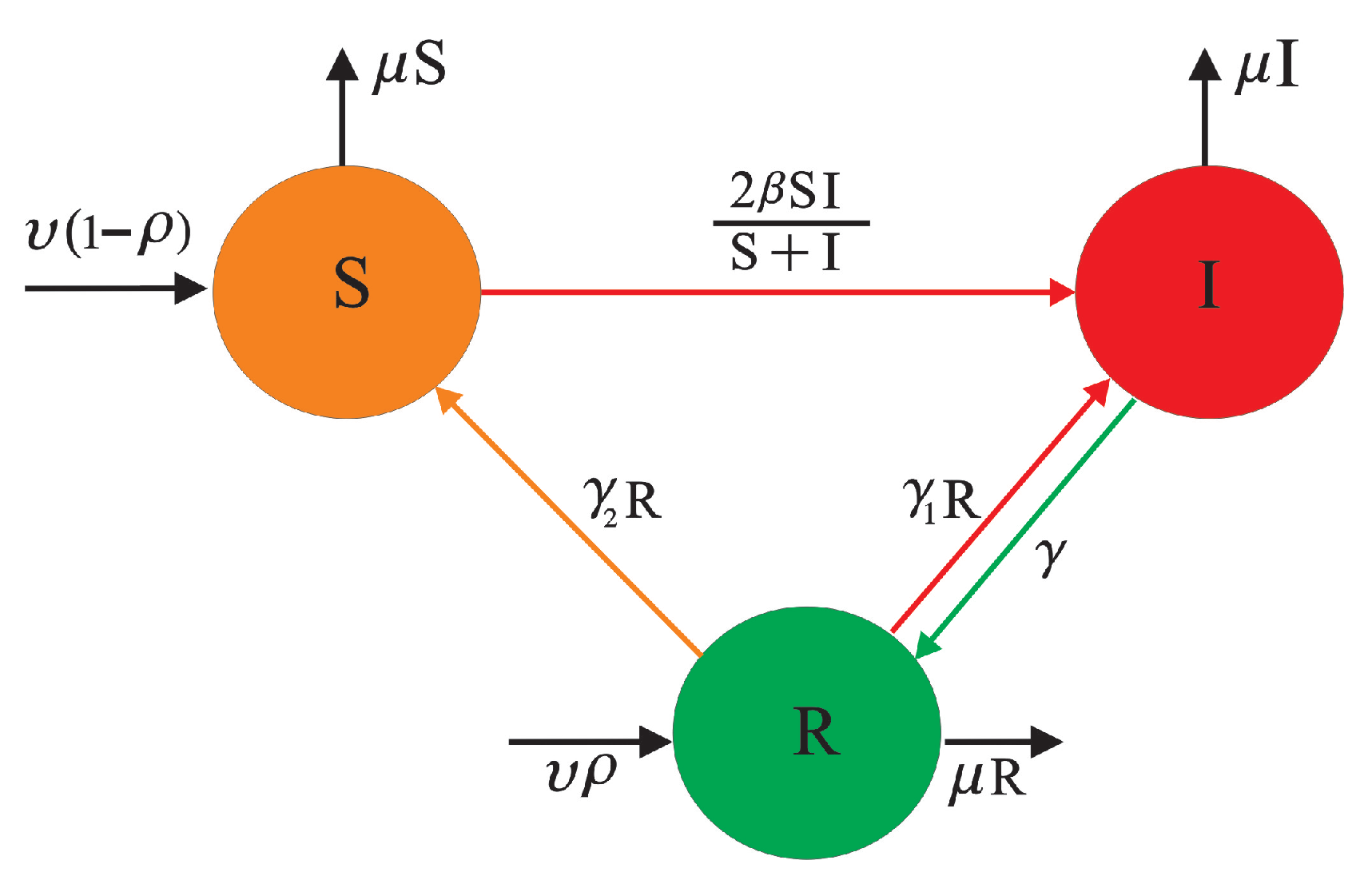
3. Model Building Process

The proposed epidemic model with harmonic mean-type incidence rate is under our investigation. For more explanation and related work, we refer the reader to [53,54,55,56,57]. The compartments and their associated differential equations collectively capture the interplay between disease transmission, recovery, and population dynamics, providing a framework for understanding and analyzing the progression of infectious diseases within a population. The following SIR epidemic model for harmonic mean-type incidence rate is constructed.

$$\left\{\begin{array}{c}\dot{\mathbf{S}}\left(t\right)=\upsilon (1-\rho )-\frac{2\beta SI}{S+I}-\mu S+{\gamma }_{2}R,\hfill \\ \dot{\mathbf{I}}\left(t\right)=\frac{2\beta SI}{S+I}-(\gamma +\mu )I+{\gamma }_{1}R,\hfill \\ \dot{\mathbf{R}}\left(t\right)=\upsilon \rho +\gamma I-({\gamma }_1+{\gamma }_2+\mu )R,\hfill \end{array}\right.$$

(10)

subject to initial conditions

$$\begin{array}{cc}& \mathbf{S}\left(0\right)={\mathbf{S}}_0,\mathbf{I}\left(0\right)={\mathbf{I}}_0,\mathbf{R}\left(0\right)={\mathbf{R}}_0.\hfill \end{array}$$

We present the schematic diagram for our model in Figure 1 as follows.

Here, the susceptible ($\mathrm{S}$) compartment encompasses individuals who have not contracted the disease, and thus, are susceptible to infection. The infected ($\mathrm{I}$) compartment comprises individuals who are currently infected with the disease. And the recovered ($\mathrm{R}$) compartment represents individuals who have recovered from the disease and have developed immunity. The notation $\beta$ stands for contact rate, $\gamma$ is the recovery rate, ${\gamma }_1$ is the reinfection rate, and $\mu$ is the natural death rate. Also, ${\gamma }_2$ is the ratio at which an immune individual becomes susceptible, $\upsilon$ is the recruitment rate, and $\rho$ is the rate at which individuals directly recur in the immune class. The primary objective of this paper is to demonstrate the existence of solutions and present numerical findings for a fractal-fractional-order SIR epidemic model with harmonic mean-type incidence rate. In Section 4, we will present the results concerning the existence of solutions for the model described by Equation (10), with our subsequent aim being to establish uniqueness. In order to accomplish this, we establish a Banach space. Let $\mathcal{B}=\mathbb{X}\times {\mathbb{R}}^3\to \mathbb{R}$ be the Banach space such that $\mathbb{X}=[0,\sigma ]$, for $0<t<\sigma <\infty$, under the norm $\parallel (\mathbf{S},\mathbf{I},\mathbf{R}\parallel ={max}_{t\in \mathbb{X}}\left\{\right|\mathbf{S}\left(t\right)|+\left|\mathbf{I}\left(t\right)\right|+\left|\mathbf{R}\left(t\right)\right|\}$.

3.1. Introduction to Equilibrium Points

This section offers an explanation of the importance of finding equilibrium points for epidemiological models and emphasizes how helpful they are in forecasting illness outcomes and planning measures to promote health. The investigation of infectious disease patterns in epidemiology is crucial for understanding the transmission and development of viral infections within populations. Equilibrium points provide useful information on the basic reproduction number, marking crucial points where confined outbreaks shift to broad epidemics. This comprehension enables healthcare authorities to predict and react to new infectious diseases before they evolve into more significant catastrophes. This type of study helps in predicting, controlling, intervening, creating policies, and implementing international health safety measures to reduce the impact of infectious disease risks.

3.2. Disease-Free Equilibrium (DFE)

To achieve DFE, we solved the system of differential equations in Equation (10) with the initial condition $I=0$, and obtained the following:

$$\begin{array}{c}\hfill E^0=\left(\frac{\upsilon (1-\rho )}{\mu },0,0\right)\end{array}$$

3.3. Endemic Equilibrium (EE)

This section outlines the process of determining the EE points by solving the equations provided in (10) that regulate the dynamics of sickness within endemic scenarios. We obtain the EE point as follows:

$$\begin{array}{c}\hfill E_1^{*}=\left(\frac{{\lambda }_1+(\mu +\gamma +{\gamma }_1+{\gamma }_2)\sqrt{{\lambda }_2}}{(\mu +{\gamma }_1+{\gamma }_2){\lambda }_3},\frac{{\lambda }_4-\sqrt{{\lambda }_2}}{{\lambda }_3},-\frac{({\lambda }_5+\gamma \sqrt{{\lambda }_2})}{(\mu +{\gamma }_1+{\gamma }_2){\lambda }_3}\right),\end{array}$$

where

$$\begin{array}{ccc}{\lambda }_1\hfill & =\hfill & -\upsilon (\mu +{\gamma }_1+{\gamma }_2)\{-(\mu +\gamma +{\gamma }_1)(-\mu (2\beta -\gamma +\mu )(-1+\rho )+(2\beta +\mu ){\gamma }_1)\hfill \\ & +\hfill & ((\gamma +\mu )\times (\gamma +\mu (-2+\rho ))-2\beta (\gamma +2\mu -\mu \rho )-(4\beta +\gamma +2\mu ){\gamma }_1){\gamma }_2\hfill \\ & -\hfill & (2\beta +\gamma +\mu ){\gamma }_2^2\},\hfill \\ {\lambda }_2\hfill & =\hfill & {\upsilon }^2{(\mu +{\gamma }_1+{\gamma }_2)}^2\{({(-2\beta +\mu )}^2+8\beta \mu \rho ){\gamma }_1^2-2(4{\beta }^2+\mu (\gamma +\mu )\hfill \\ & -\hfill & 2\beta (\gamma +2\mu -2\mu \rho )){\gamma }_1(\mu (-1+\rho )-{\gamma }_2)+{(-2\beta +\gamma +\mu )}^2{(\mu -\mu \rho +{\gamma }_2)}^2\},\hfill \\ {\lambda }_3\hfill & =\hfill & 2\mu \left\{2\beta {\gamma }_1^2+(\mu +{\gamma }_2)((2\beta -\gamma )(\gamma +\mu )+2\beta {\gamma }_2)+{\gamma }_1(2\beta \gamma +4\beta \mu -\gamma \mu +4\beta {\gamma }_2)\right\},\hfill \\ {\lambda }_4\hfill & =\hfill & (2\beta -\mu )\upsilon {\gamma }_1^2-(2\beta -\gamma -\mu )\upsilon (\mu (-1+\rho )-{\gamma }_2)(\mu +{\gamma }_2)\hfill \\ & +\hfill & \upsilon {\gamma }_1\left\{-\mu (\gamma +2\mu +2\beta (-2+\rho )+\gamma \rho -\mu \rho )+(4\beta -\gamma -2\mu ){\gamma }_2\right\},\hfill \\ {\lambda }_5\hfill & =\hfill & \upsilon (\mu +{\gamma }_1+{\gamma }_2)\{\mu (\gamma (\gamma +\mu )(1+\rho )-2\beta (\gamma +\gamma \rho +2\mu \rho ))+(\gamma \mu -2\beta (\gamma +2\mu \rho )){\gamma }_1\hfill \\ & +\hfill & (\gamma (\gamma +\mu )-2\beta (\gamma +2\mu \rho )){\gamma }_2\}.\hfill \end{array}$$

and

$$\begin{array}{c}\hfill E_2^{*}=\left(-\frac{{\lambda }_1^{\prime }+(\mu +\gamma +{\gamma }_1+{\gamma }_2)\sqrt{{\lambda }_2}}{(\mu +{\gamma }_1+{\gamma }_2){\lambda }_3},\frac{{\lambda }_4+\sqrt{{\lambda }_2}}{{\lambda }_3},\frac{({\lambda }_5^{\prime }+\gamma \sqrt{{\lambda }_2})}{(\mu +{\gamma }_1+{\gamma }_2){\lambda }_3}\right),\end{array}$$

where

$$\begin{array}{ccc}\hfill {\lambda }_1^{\prime }& =& \upsilon (\mu +{\gamma }_1+{\gamma }_2)\{-(\mu +\gamma +{\gamma }_1)(-\mu (2\beta -\gamma +\mu )(-1+\rho )+(2\beta +\mu ){\gamma }_1)\hfill \\ & +& ((\gamma +\mu )(\gamma +\mu (-2+\rho ))-2\beta (\gamma +2\mu -\mu \rho )-(4\beta +\gamma +2\mu ){\gamma }_1){\gamma }_2\hfill \\ & -& (2\beta +\gamma +\mu ){\gamma }_2^2\},\hfill \\ \hfill {\lambda }_5^{\prime }& =& -\upsilon (\mu +{\gamma }_1+{\gamma }_2)\{\mu (\gamma (\gamma +\mu )(1+\rho )-2\beta (\gamma +\gamma \rho +2\mu \rho ))\hfill \\ & +& (\gamma \mu -2\beta (\gamma +2\mu \rho )){\gamma }_1+\gamma (\gamma +\mu )-2\beta (\gamma +2\mu \rho )){\gamma }_2\}.\hfill \end{array}$$

3.4. Fundamental Number $R_0$

We compute the reproductive number $R_0$ by applying the next-generation matrix approach. This analytical approach provides insights into the potential spread and dynamics of infectious diseases within populations. We see that S and R are the healthy classes of the population in system (10), so by selecting the compartments where infection exists, we have

$$\begin{array}{c}\hfill \dot{\mathbf{I}}\left(t\right)=\frac{2\beta SI}{S+I}-(\gamma +\mu )I+{\gamma }_{1}R.\end{array}$$

(11)

Let $X=\left(I\right)$, then from system (11) we have

$$\frac{dX}{dt}=\mathbb{F}-\mathbb{V},$$

where

$$\mathbb{F}=\frac{2\beta SI}{S+I}\mathrm{and}\mathbb{V}=(\gamma +\mu )I-{\gamma }_{1}R.$$

Let F and V represent the partial derivative of $\mathbb{F}$ and $\mathbb{V}$ at DFE, respectively, then

$$F=\frac{\partial \mathbb{F}}{\partial I}=2\beta \mathrm{and}V=\frac{\partial \mathbb{V}}{\partial I}=(\mu +\gamma ).$$

Furthermore,

$$V^{-1}=\frac{1}{\mu +\gamma },$$

so,

$$F{V}^{-1}=\frac{2\beta }{(\mu +\gamma )}.$$

Thus, the basic reproductive number is computed as follows:

$$R_0=\frac{2\beta }{(\mu +\gamma )}.$$

3.5. Sensitivity Analysis

In this section, we delve into sensitivity analysis to understand how our model reacts to fluctuations in parameter values, with a specific focus on identifying the parameters that significantly affect disease transmission, notably the reproductive number ($R_0$). To undertake this analysis, we utilize the normalized forward sensitivity index method, as detailed in [58]. This method involves determining the ratio of the relative change in a variable to the relative change in the corresponding parameter. Alternatively, sensitivity indices can be computed using partial derivatives when the variable is a differentiable function of the parameter.

Hence, in our proposed model, we provide the normalized forward sensitivity index for $R_0$ utilizing the specified approach.

$$\begin{array}{c}\hfill S_n^{R_0}=\left[\frac{\partial R_0}{\partial n}\right]\times \frac{n}{R_0}.\end{array}$$

$$\begin{array}{cc}\hfill S_{\beta }^{R_0}& =\frac{\beta }{R_0}\frac{2}{\mu +\gamma }=1>0,\hfill \\ \hfill S_{\gamma }^{R_0}& =-\frac{\mu }{(\gamma +\mu )}=-0.00000714<0,\hfill \\ \hfill S_{\mu }^{R_0}& =-\frac{\beta }{(\gamma +\mu )}=-0.52448<0.\hfill \end{array}$$

(12)

Based on the normalized forward sensitivity index, presented in (12), it seems that the parameter $\beta$ is the most sensitive for the transmission of the disease. This is inferred from the fact that the sensitivity coefficient for $\beta$, $S_{\beta }^{R_0}$ is positive, indicating that an increase in $\beta$ leads to an increase in the basic reproduction number $R_0$. On the other hand, the sensitivity coefficients for $\gamma$ and $\mu$ are negative, suggesting that an increase in either $\gamma$ or $\mu$ would decrease the value of $R_0$. However, since $\beta$ has a positive sensitivity coefficient while $\gamma$ and $\mu$ have negative sensitivity coefficients of the same magnitude, the impact of changes in $\beta$ is likely to be more pronounced in affecting the transmission dynamics of the disease.

Therefore, we have the following theorem

Theorem 1.

If $R_0\le 1$, the system does not possess positive equilibrium points. Conversely, for $R_0>1$, a unique positive equilibrium point $E^{*}$ arises within the model (10), recognized as the endemic equilibrium.

In the forthcoming theorem, we demonstrate that the model (10) consistently yields non-negative solutions for all primary values.

Theorem 2.

The solutions to the system described by Equation (10) become ultimately restricted within a bounded region for all $t\ge 0$. The bounded region, denoted as ∁, is given below:

$$\complement =\left\{\left(S,I,R\right)\in {\mathbf{R}}_{+}^3:0<N\left(t\right)\le \frac{\upsilon }{\mu },S\le S_0\right\}.$$

Proof. 

Assume $\left(S\left(t\right),I\left(t\right),R\left(t\right)\right)$ as the general solution of system (10) under the non-negative initial conditions. Considering $N\left(t\right)=S\left(t\right)+I\left(t\right)+R\left(t\right)$ as the total population excluding individuals in the deceased category, we observe that

$$\frac{dN}{dt}=\frac{dS}{dt}+\frac{dI}{dt}+\frac{dR}{dt}.$$

(13)

For simplicity, we adopt $(N,S,I,R)$ in place of $\left(N\right(t),S(t),I(t),R(t\left)\right)$, respectively. Utilizing the values from Equation (10), it follows from (13) that

$$\begin{array}{ccc}\hfill \frac{dN}{dt}& =& \upsilon (1-\rho )-\frac{2\beta SI}{S+I}-\mu S+{\gamma }_{2}R+\frac{2\beta SI}{S+I}\hfill \\ & -& (\gamma +\mu )I+{\gamma }_{1}R+\nu \rho +\gamma I-({\gamma }_1+{\gamma }_2+\mu )R\hfill \\ & =& \upsilon \rho -\mu (S+I+R)\hfill \\ & =& \upsilon -\mu N.\hfill \end{array}$$

(14)

From (14), we obtain

$$\begin{array}{c}\hfill \frac{dN}{dt}+\mu N=\upsilon ,\end{array}$$

(15)

which is a linear differential equation having the integrating factor ($I.F$) $I.F=exp\left(\mu t\right)$; multiplication by $I.F$ (16) implies that

$$\begin{array}{c}\hfill exp\left(\mu t\right)\frac{dN}{dt}+exp\left(\mu t\right)\mu N=\upsilon exp\left(\mu t\right)\end{array}$$

which can be written as follows:

$$\begin{array}{c}\hfill \frac{d}{dt}\left[Nexp\left(\mu t\right)\right]=\upsilon exp\left(\mu t\right).\end{array}$$

On solving, we have

$$N\left(t\right)=\frac{\upsilon }{\mu }+N_{0}exp(-\mu t).$$

(16)

Here, $N_0$ is the initial population.

As t approaches infinity in Equation (16), it becomes evident that $N\left(t\right)$ remains bounded by $\frac{\upsilon }{\mu }$. Consequently, the desired feasible region is established.

In addition, it follows that

$$\underset{t\to \infty }{lim}supN\le N_0,\mathrm{with}\underset{t\to \infty }{lim}supN=N_0,$$

only when

$$\underset{t\to \infty }{lim}supI=0.$$

Following the first and second equations of the model (10), it can be deduced that

$$0\le \underset{t\to \infty }{lim}supS\le S_0.$$

Therefore, based on the preceding analysis, it is evident that when $N>N_0$, the rate of change of N, that is, $\frac{dN}{dt}$, is negative. Consequently, the solutions of system (10) are ultimately positive and bounded within the compact subset ∁ for all $t\ge 0$, implying that the solutions of the model (10) always remain within the interval $[0,\infty )$. □

3.6. Local Stability of DFE and EE

In the study and analysis of dynamical systems, the Hartman–Grobman theorem plays a crucial role in determining the stability of the equilibrium points in a nonlinear system by analyzing the eigenvalues of the linearized system near these points. This allows for the classification of equilibrium points as stable, unstable, or neutrally stable. Thus, the subsequent theorem is cited in this context.

Theorem 3

([59,60]). If the Jacobian matrix of a dynamical system evaluated at a critical point (equilibrium point) has eigenvalues with negative real parts, then the system is locally asymptotically stable around that equilibrium point.

The above theorem is crucial in nonlinear dynamics because it allows us to analyze the stability of nonlinear systems by linearizing them around equilibrium points and examining the resulting linear system’s behavior. The negative real parts of the eigenvalues imply that the linearized system is stable, indicating that the original nonlinear system exhibits stable behavior locally around the equilibrium point.

Theorem 4.

System (10) exhibits local asymptotic stability around $E^0$ if $R_0<1$.

Proof. 

The Jacobian matrix of system (10) at $E^0$ can be obtained as

$J^0=\left[\begin{array}{ccc}-\mu & -2\beta & {\gamma }_2\\ 0& 2\beta -(\gamma +\mu )& {\gamma }_1\\ 0& \gamma & -({\gamma }_1+{\gamma }_2+\mu )\end{array}\right]$.

The eigenvalues of the Jacobian matrix $J^0$ are as follows:

$$\begin{array}{c}\hfill \left\{\begin{array}{c}{\lambda }_1=-\mu ,\hfill \\ {\lambda }_2=\frac{(\mu +\gamma )(R_0-1)-(\mu +{\gamma }_1+{\gamma }_2)-\sqrt{{\gamma }_1^2+{(2\beta -\gamma +{\gamma }_2)}^2+2{\gamma }_1(2\beta +\gamma +{\gamma }_2)}}{2},\hfill \\ {\lambda }_3=\frac{(\mu +\gamma )(R_0-1)-(\mu +{\gamma }_1+{\gamma }_2)+\sqrt{{\gamma }_1^2+{(2\beta -\gamma +{\gamma }_2)}^2+2{\gamma }_1(2\beta +\gamma +{\gamma }_2)}}{2}.\hfill \end{array}\right.\end{array}$$

(17)

We have observed that all eigenvalues have negative real parts when $R_0<1$. Utilizing Theorem 3, this implies that under the condition $R_0<1$, the system described by Equation (10) achieves local asymptotic stability at the disease-free equilibrium $E^0$. Hence, this completes the proof. □

Theorem 5.

System (10) exhibits local asymptotic stability around each $E_i^{*}$ if $R_0<1$.

Proof. 

The Jacobian matrix of system (10) at each $E_i^{*}$ can be obtained as

$J^{*}=\left[\begin{array}{ccc}-2\beta {\left(\frac{I^{*}}{S^{*}+I^{*}}\right)}^2-\mu & -2\beta {\left(\frac{S^{*}}{S^{*}+I^{*}}\right)}^2& {\gamma }_2\\ -2\beta {\left(\frac{I^{*}}{S^{*}+I^{*}}\right)}^2& 2\beta {\left(\frac{S^{*}}{S^{*}+I^{*}}\right)}^2-(\gamma +\mu )& {\gamma }_1\\ 0& \gamma & -({\gamma }_1+{\gamma }_2+\mu )\end{array}\right]$.

The eigenvalues of the Jacobian matrix $J^{*}$ are as follows:

$$\begin{array}{c}\hfill \left\{\begin{array}{c}{\lambda }_1=-\mu ,\hfill \\ {\lambda }_2=-\frac{(2\mu +\gamma +{\gamma }_1+{\gamma }_2)}{2}+\frac{2\beta (S^{*}-I^{*})-\sqrt{\mathbb{k}}}{2(S^{*}+I^{*})},\hfill \\ {\lambda }_3=\frac{S^{*}(\gamma +\mu )\left((R_0-1)-\frac{\mu }{\gamma +\mu }\right)-I^{*}(2\beta +\gamma +2\mu )}{2(S^{*}+I^{*})}-\frac{(S^{*}+I^{*})({\gamma }_1+{\gamma }_2)\sqrt{\mathbb{k}}}{2(S^{*}+I^{*})}.\hfill \end{array}\right.\end{array}$$

Here,

$$\begin{array}{ccc}\hfill \mathbb{k}& =& 4{(S^{*}-I^{*})}^2{\beta }^2-4({\left(S^{*}\right)}^2+{\left(I^{*}\right)}^2)\beta \gamma +4(S^{*}-I^{*})(S^{*}+I^{*})(\beta {\gamma }_1+\beta {\gamma }_2)\hfill \\ & +& {(S^{*}+I^{*})}^2\left({\gamma }^2+2\gamma {\gamma }_1+{\gamma }_1^2-2\gamma {\gamma }_2+2{\gamma }_1{\gamma }_2+{\gamma }_2^2\right)\hfill \end{array}$$

We have observed that all eigenvalues have negative real parts when $R_0<1$. Utilizing Theorem 3, this implies that under the condition $R_0<1$, the system described by Equation (10) achieves local asymptotic stability at each endemic equilibrium $E_i^{*}$. Hence, this completes the proof. □

3.7. Global Stability of DFE at $E^0$

We employ the same methodology as utilized in [61] to obtain the necessary outcomes for global asymptotic stability.

Theorem 6.

System (10) is globally asymptotically stable at $E^0=\left(\frac{\upsilon (1-\rho )}{\mu },0,0\right)$.

Proof. 

Taking the Lyapunov function corresponding to all dependent classes of the model:

$$L=k_1(S-S^{*})+k_2(I-I^{*})+k_3(R-R^{*}).$$

Differentiating with respect to t we obtain

$$L^{\prime }=k_1{S}^{\prime }+k_2{I}^{\prime }+k_3{R}^{\prime }.$$

After utilizing the values derived from system (10) and performing the requisite calculations, we obtain

$$\begin{array}{ccc}\hfill L^{\prime }& =& k_1\left[\upsilon (1-\rho )-\frac{2\beta SI}{S+I}-\mu S+{\gamma }_{2}R\right]+k_2\left[\frac{2\beta SI}{S+I}-(\gamma +\mu )I+{\gamma }_{1}R\right]\hfill \\ & +& k_3\left[\upsilon \rho +\gamma I-({\gamma }_1+{\gamma }_2+\mu )R\right]\hfill \\ & =& k_1\upsilon +(k_3-k_1)\upsilon \rho +(k_2-k_1)\frac{2\beta SI}{S+I}+(k_1-k_3){\gamma }_{2}R+(k_3-k_2)\gamma I\hfill \\ & +& (k_2-k_3){\gamma }_{1}R-k_1\mu S-k_2\mu I-k_3\mu R\hfill \end{array}$$

Since $k_1$, $k_2$, and $k_3$ are arbitrary constants. So, for simplicity, assume that $k_1=1$, $k_2=1$, and $k_3=1$. Thus,

$$\begin{array}{ccc}\hfill L^{\prime }& =& \upsilon -\mu S-\mu I-\mu R\hfill \\ & =& \upsilon -\mu (S+I+R)\hfill \\ & =& (\upsilon -\mu N)<0.\hfill \end{array}$$

Hence, system (10) is globally asymptotically stable at $E_0$. □

Global Stability Analysis of EE at $E^{*}$

In order to attain the global stability at $E^{*}$, we utilize the following Lyapunov function.

$$L=k_1{(S-S^{*})}^2+2k_2{(I-I^{*})}^2+k_3{(R-R^{*})}^2.$$

Here, $k_1$, $k_2$, and $k_3$ are all positive. Taking the derivative of L and using the values of $S^{\prime }$, $I^{\prime }$, and $R^{\prime }$ from (10), we obtain

$$\begin{array}{c}\hfill L^{\prime }=2k_1(S-S^{*})S^{\prime }+2k_2(I-I^{*})I^{\prime }+2k_3(R-R^{*})R^{\prime }.\end{array}$$

Here,

$$\begin{array}{ccc}\hfill 2k_1(S-S^{*})S^{\prime }& =\hfill & 2k_1(S-S^{*})\left[-\frac{2\beta SI}{S+I}+\frac{2\beta S^{*}{I}^{*}}{S^{*}+I^{*}}-\mu S+\mu S^{*}+{\gamma }_{2}R-{\gamma }_2{R}^{*}\right]\hfill \\ & =\hfill & 2k_1(S-S^{*})\left[-\left\{\frac{2\beta I}{S+I}+\mu \right\}S+\left\{\frac{2\beta I^{*}}{S^{*}+I^{*}}+\mu \right\}{S}^{*}+{\gamma }_2(R-R^{*})\right]\hfill \\ & =\hfill & 2k_1(S-S^{*})\left[-AS+B{S}^{*}+{\gamma }_2(R-R^{*})\right]\hfill \\ & =\hfill & 2k_1(S-S^{*})\left[-AS+A{S}^{*}-A{S}^{*}+B{S}^{*}+{\gamma }_2(R-R^{*})\right]\hfill \\ & =\hfill & 2k_1(S-S^{*})\left[-A(S-S^{*})-(A-B)S^{*}+{\gamma }_2(R-R^{*})\right]\hfill \\ & =\hfill & 2k_1(S-S^{*})[\left\{-A+\frac{2\beta S^{*}{I}^{*}}{(S+I)(S^{*}+I^{*})}\right\}(S-S^{*})\hfill \\ & -\hfill & \frac{2\beta {\left(S^{*}\right)}^2}{(S+I)(S^{*}+I^{*})}(I-I^{*})+{\gamma }_2(R-R^{*})],\hfill \\ \hfill 2k_2(I-I^{*})I^{\prime }& =\hfill & 2k_2(I-I^{*})\left[\frac{2\beta SI}{S+I}-\frac{2\beta S^{*}{I}^{*}}{S^{*}+I^{*}}-(\gamma +\mu )I+(\gamma +\mu )I^{*}+{\gamma }_{1}R-{\gamma }_1{R}^{*}\right]\hfill \\ & =\hfill & 2k_2(I-I^{*})\left[\left\{\frac{2\beta S}{S+I}-(\gamma +\mu )\right\}I-\left\{\frac{2\beta S^{*}}{S^{*}+I^{*}}-(\gamma +\mu )\right\}{I}^{*}+{\gamma }_1(R-R^{*})\right]\hfill \\ & =\hfill & 2k_2(I-I^{*})\left[CI-D{I}^{*}+{\gamma }_1(R-R^{*})\right]\hfill \\ & =\hfill & 2k_2(I-I^{*})\left[CI-C{I}^{*}+C{I}^{*}-D{I}^{*}+{\gamma }_1(R-R^{*})\right]\hfill \\ & =\hfill & 2k_2(I-I^{*})\left[C(I-I^{*})+(C-D)I^{*}+{\gamma }_1(R-R^{*})\right]\hfill \\ & =\hfill & 2k_2(I-I^{*})[\left\{C-\frac{2\beta S^{*}{I}^{*}}{(S+I)(S^{*}+I^{*})}\right\}(I-I^{*})+\frac{2\beta {\left(I^{*}\right)}^2}{(S+I)(S^{*}+I^{*})}(S-S^{*})\hfill \\ & +\hfill & {\gamma }_1(R-R^{*})],\mathrm{and}\hfill \\ 2k_2(I-I^{*})I^{\prime }& =& 2k_3(R-R^{*})\left[\gamma (I-I^{*})-({\gamma }_1+{\gamma }_2+\mu )(R-R^{*})\right]\hfill \\ \hfill \Rightarrow L^{\prime }& =& P(KJ+J^{T}K)P^T.\hfill \end{array}$$

Here, $P=[S-S^{*},I-I^{*},R-R^{*}]$, $K=\mathbf{diag}(k_1,k_2,k_3)$ and

$$J=\left[\begin{array}{ccc}-A+\frac{2\beta S^{*}{I}^{*}}{(S+I)(S^{*}+I^{*})}& -\frac{2\beta {\left(S^{*}\right)}^2}{(S+I)(S^{*}+I^{*})}& {\gamma }_2\\ \frac{2\beta {\left(I^{*}\right)}^2}{(S+I)(S^{*}+I^{*})}& C-\frac{2\beta S^{*}{I}^{*}}{(S+I)(S^{*}+I^{*})}& {\gamma }_1\\ 0& \gamma & -({\gamma }_1+{\gamma }_2+\mu )\end{array}\right].$$

(18)

Claim 1.

The inequality $\frac{2\beta I}{S+I}+\mu -\frac{2\beta S^{*}{I}^{*}}{(S+I)(S^{*}+I^{*})}>0$ always holds true.

Proof. 

For convenience, let $\mathbf{a}=2\beta$, $\mathbf{b}=I$, $\mathbf{c}=S+I$, $\mathbf{d}=S^{*}$, and $\mathbf{e}=I^{*}$. Then,

$$\begin{array}{ccc}\hfill \frac{2\beta I}{S+I}+\mu -\frac{2\beta S^{*}{I}^{*}}{(S+I)(S^{*}+I^{*})}& =& \left\{\frac{2\beta I}{S+I}-\frac{2\beta S^{*}{I}^{*}}{(S+I)(S^{*}+I^{*})}\right\}+\mu \hfill \\ & =& \left\{\frac{\mathbf{a}\mathbf{b}}{\mathbf{c}}-\frac{\mathbf{a}\mathbf{d}\mathbf{e}}{\mathbf{c}(\mathbf{d}+\mathbf{e})}\right\}+\mu \hfill \\ & =& \left\{\frac{\mathbf{a}\mathbf{b}(\mathbf{d}+\mathbf{e})-\mathbf{a}\mathbf{d}\mathbf{e}}{\mathbf{c}(\mathbf{d}+\mathbf{e})}\right\}+\mu \hfill \\ & =& \left\{\frac{\mathbf{a}\mathbf{b}\mathbf{d}+\mathbf{a}\mathbf{b}\mathbf{e}-\mathbf{a}\mathbf{d}\mathbf{e}}{\mathbf{c}(\mathbf{d}+\mathbf{e})}\right\}+\mu \hfill \\ & =& \left\{\frac{\mathbf{a}\mathbf{b}\mathbf{e}+\mathbf{a}\mathbf{d}(\mathbf{b}-\mathbf{e})}{\mathbf{c}(\mathbf{d}+\mathbf{e})}\right\}+\mu \hfill \end{array}$$

Since $\mathbf{b}-\mathbf{e}=I-I^{*}\ge 0$ because $I\ge I^{*}$. This implies that $\mathbf{a}\mathbf{b}\mathbf{e}+\mathbf{a}\mathbf{d}(\mathbf{b}-\mathbf{e})>0$, which means that $\frac{2\beta I}{S+I}+\mu -\frac{2\beta S^{*}{I}^{*}}{(S+I)(S^{*}+I^{*})}>0$. This completes the proof of our claim. □

Claim 2.

The inequality $-\frac{2\beta S}{S+I}+(\gamma +\mu )+\frac{2\beta S^{*}{I}^{*}}{(S+I)(S^{*}+I^{*})}>0$ always holds true when  $R_0<1$ and $0<\frac{S}{S+I}<1$.

Proof. 

$$\begin{array}{ccc}-\frac{2\beta S}{S+I}+(\gamma +\mu )+\frac{2\beta S^{*}{I}^{*}}{(S+I)(S^{*}+I^{*})}\hfill & =\hfill & -\left\{\frac{2\beta S}{S+I}-(\gamma +\mu )\right\}+\frac{2\beta S^{*}{I}^{*}}{(S+I)(S^{*}+I^{*})}\hfill \\ \hfill & =\hfill & -(\gamma +\mu )\left\{\left(\frac{S}{S+I}\right)\left(\frac{2\beta }{\gamma +\mu }\right)-1\right\}\hfill \\ & +\hfill & \frac{2\beta S^{*}{I}^{*}}{(S+I)(S^{*}+I^{*})}\hfill \\ \hfill & =\hfill & -(\gamma +\mu )\left\{\left(\frac{S}{S+I}\right)R_0-1\right\}+\frac{2\beta S^{*}{I}^{*}}{(S+I)(S^{*}+I^{*})}.\hfill \end{array}$$

Since we see that $\left(\frac{S}{S+I}\right)R_0-1<0$ when $R_0<1$ and $0<\frac{S}{S+I}<1$. This implies that

$$-(\gamma +\mu )\left\{\left(\frac{S}{S+I}\right)R_0-1\right\}>0,$$

which means that $-\frac{2\beta S}{S+I}+(\gamma +\mu )>0$. Therefore, the inequality $-\frac{2\beta S}{S+I}+(\gamma +\mu )+$$\frac{2\beta S^{*}{I}^{*}}{(S+I)(S^{*}+I^{*})}>0$ always holds true when $R_0<1$ and $0<\frac{S}{S+I}<1$. This completes the proof of our claim. □

Claim 3.

If $a=A-\frac{2\beta S^{*}{I}^{*}}{(S+I)(S^{*}+I^{*})}$, $b=\frac{2\beta {\left(S^{*}\right)}^2}{(S+I)(S^{*}+I^{*})}$, $c={\gamma }_2$, $d=\frac{2\beta {\left(I^{*}\right)}^2}{(S+I)(S^{*}+I^{*})}$, $e=-C+\frac{2\beta S^{*}{I}^{*}}{(S+I)(S^{*}+I^{*})}$, $f={\gamma }_1$, $g=\gamma$, and $h=({\gamma }_1+{\gamma }_2+\mu )$, then,

(i) 

$-fg+eh>0$;

(ii) 

$-cg+bh>0$;

(iii) 

$cg-bh<0$.

Proof. 

(i)

$-fg+eh>0$

$$\begin{array}{ccc}\hfill eh-fg& =& \left(-C+\frac{2\beta S^{*}{I}^{*}}{(S+I)(S^{*}+I^{*})}\right)\left({\gamma }_1+{\gamma }_2+\mu \right)-{\gamma }_1\gamma \hfill \\ & =& \left(-\frac{2\beta S}{S+I}+(\gamma +\mu )+\frac{2\beta S^{*}{I}^{*}}{(S+I)(S^{*}+I^{*})}\right)\left({\gamma }_1+{\gamma }_2+\mu \right)-\gamma {\gamma }_1\hfill \\ & =& -\frac{2\beta S\left({\gamma }_1+{\gamma }_2+\mu \right)}{S+I}+(\gamma +\mu )\left({\gamma }_1+{\gamma }_2+\mu \right)+\frac{2\beta S^{*}{I}^{*}\left({\gamma }_1+{\gamma }_2+\mu \right)}{(S+I)(S^{*}+I^{*})}-\gamma {\gamma }_1\hfill \\ & =& -\frac{2\beta S\left({\gamma }_1+{\gamma }_2+\mu \right)}{S+I}+\mu \gamma {\gamma }_1+\mu \gamma {\gamma }_2+\mu \gamma \mu +\frac{2\beta S^{*}{I}^{*}\left({\gamma }_1+{\gamma }_2+\mu \right)}{(S+I)(S^{*}+I^{*})}-\gamma {\gamma }_1.\hfill \end{array}$$

Based on Claim 2, $-\frac{2\beta S}{S+I}+(\gamma +\mu )+\frac{2\beta S^{*}{I}^{*}}{(S+I)(S^{*}+I^{*})}>0$ when $R_0<1$ and $0<\frac{S}{S+I}<1$. Moreover, one can easily see that $\mu \gamma {\gamma }_1+\mu \gamma {\gamma }_2+\mu \gamma \mu >\gamma {\gamma }_1$; therefore, $-fg+eh>0$.

(ii)

$-cg+bh>0$

$$\begin{array}{ccc}\hfill bh-cg& =& \left(\frac{2\beta {\left(S^{*}\right)}^2}{(S+I)(S^{*}+I^{*})}\right)\left({\gamma }_1+{\gamma }_2+\mu \right)-{\gamma }_2\gamma \hfill \\ & =& \left(\frac{2\beta {\left(S^{*}\right)}^2}{(S+I)(S^{*}+I^{*})}\right)\left({\gamma }_1+{\gamma }_2+\mu \right)-(\gamma +\mu ){\gamma }_2+\mu {\gamma }_2.\hfill \\ & =& \left\{\left(\frac{{\left(S^{*}\right)}^2\left({\gamma }_1+{\gamma }_2+\mu \right)}{{\gamma }_2(S+I)(S^{*}+I^{*})}\right)\left(\frac{2\beta }{\gamma +\mu }\right)-1\right\}+\mu {\gamma }_2\hfill \\ & =& \left\{\left(\frac{{\left(S^{*}\right)}^2\left({\gamma }_1+{\gamma }_2+\mu \right)}{{\gamma }_2(S+I)(S^{*}+I^{*})}\right)R_0-1\right\}+\mu {\gamma }_2.\hfill \end{array}$$

It is easy to see that when $R_0<1$ and $\left(\frac{{\left(S^{*}\right)}^2({\gamma }_1+{\gamma }_2+\mu )}{{\gamma }_2(S+I)(S^{*}+I^{*})}\right)>\frac{28}{25}$, then $-cg+bh>0$.

(iii)

$cg-bh<0$

Based on $-cg+bh>0$, we can easily see that $cg-bh=-(-cg+bh)<0$. This completes the proof of all parts of our claim. □

Theorem 7.

The matrix J is V-L stable.

Proof. 

Clearly $-J_{33}>0$. Consider $\mathbf{D}=-\tilde{J}$ to be a $2\times 2$ matrix obtained by deleting the last column and row of the matrix $-J$. To prove that the matrix J is V-L stable, it is necessary to show that $\mathbf{D}=-\tilde{J}$ and $\mathbf{H}=-\widetilde{J^{-1}}$ are both diagonal stable. For this, from matrix A, we obtain

$$\mathbf{D}=-\tilde{J}=\left[\begin{array}{cc}A-\frac{2\beta S^{*}{I}^{*}}{(S+I)(S^{*}+I^{*})}& \frac{2\beta {\left(S^{*}\right)}^2}{(S+I)(S^{*}+I^{*})}\\ -\frac{2\beta {\left(I^{*}\right)}^2}{(S+I)(S^{*}+I^{*})}& -C+\frac{2\beta S^{*}{I}^{*}}{(S+I)(S^{*}+I^{*})}\end{array}\right].$$

Based on Claim 1 and Claim 2, one can easily see that

$${\mathbf{D}}_{\mathbf{11}}>0\mathrm{and}{\mathbf{D}}_{\mathbf{22}}>0,$$

moreover, it is obvious that

$${\mathbf{D}}_{\mathbf{12}}>0\mathrm{and}{\mathbf{D}}_{\mathbf{21}}<0.$$

Therefore, $det\left(\mathbf{D}\right)={\mathbf{D}}_{\mathbf{11}}{\mathbf{D}}_{\mathbf{22}}-{\mathbf{D}}_{\mathbf{21}}{\mathbf{D}}_{\mathbf{12}}>0.$ This shows that $\mathbf{D}$ is diagonal stable. It is now necessary to show that $\mathbf{H}=-\widetilde{J^{-1}}$ is diagonal stable. Regarding this, we have

$$-J=\left[\begin{array}{ccc}A-\frac{2\beta S^{*}{I}^{*}}{(S+I)(S^{*}+I^{*})}& \frac{2\beta {\left(S^{*}\right)}^2}{(S+I)(S^{*}+I^{*})}& -{\gamma }_2\\ -\frac{2\beta {\left(I^{*}\right)}^2}{(S+I)(S^{*}+I^{*})}& -C+\frac{2\beta S^{*}{I}^{*}}{(S+I)(S^{*}+I^{*})}& -{\gamma }_1\\ 0& -\gamma & ({\gamma }_1+{\gamma }_2+\mu )\end{array}\right].$$

For convenience, let us consider $a=A-\frac{2\beta S^{*}{I}^{*}}{(S+I)(S^{*}+I^{*})}$, $b=\frac{2\beta {\left(S^{*}\right)}^2}{(S+I)(S^{*}+I^{*})}$, $c={\gamma }_2$, $d=\frac{2\beta {\left(I^{*}\right)}^2}{(S+I)(S^{*}+I^{*})}$, $e=-C+\frac{2\beta S^{*}{I}^{*}}{(S+I)(S^{*}+I^{*})}$, $f={\gamma }_1$, $g=\gamma$, and $h=({\gamma }_1+{\gamma }_2+\mu ),$ the same as mentioned in Claim 3, Then,

$$-J=\left[\begin{array}{ccc}a& b& -c\\ -d& e& -f\\ 0& -g& h\end{array}\right].$$

Therefore,

$${(-J)}^{-1}=\frac{1}{\left\{(-cg+bh)d+(-fg+eh)a\right\}}\left[\begin{array}{ccc}-fg+eh& cg-bh& ce-bf\\ dh& ah& cd+af\\ dg& ag& bd+ae\end{array}\right].$$

Based on Claim 3, we see that $det(-J)=\left\{(-cg+bh)d+(-fg+eh)a\right\}>0$, also it is obvious that $bd+ae>0$. Therefore, ${(-J)}_{33}^{-1}>0$. Now, we need to show that $H=\widetilde{{(-J)}^{-1}}$ is diagonal stable. For this,

$$H=\widetilde{{(-J)}^{-1}}=\frac{1}{\left\{(-cg+bh)d+(-fg+eh)a\right\}}\left[\begin{array}{cc}-fg+eh& cg-bh\\ dh& ah\end{array}\right].$$

Based on Claim 3, we can see that

$$H_{11}>0\mathrm{and}{H}_{22}>0,$$

moreover,

$$H_{21}>0\mathrm{and}{H}_{12}<0.$$

Thus, $det\left(H\right)=H_{11}{H}_{22}-H_{21}{H}_{12}>0$; therefore, H is diagonal stable. Thus, based on Lemma 1 and Lemma 2, the matrix J defined in Equation (18) is V-L stable. □

In summary of the preceding discussions, we have drawn these conclusions regarding the global asymptotic stability of the EE.

Theorem 8.

When $R_0>1$, the endemic equilibrium $E^{*}=(S^{*},I^{*},R^{*})$ in model (10) exhibits global asymptotic stability within ∁.

Proof. 

Based on Theorem 7, it is assured that the EE of model (10) achieves global asymptotic stability at $E^{*}$. □

4. Fractal-Fractional Model Formulation and Methodology

We rewrite Equation (10) incorporating the fractal-fractional derivative as follows:

$$\left\{\begin{array}{c}{ }^{FFM}{\mathbb{D}}_{0,t}^{\epsilon ,\delta }\left(\mathbf{S}\left(t\right)\right)=\upsilon (1-\rho )-\frac{2\beta SI}{S+I}-\mu S+{\gamma }_{2}R,\hfill \\ { }^{FFM}{\mathbb{D}}_{0,t}^{\epsilon ,\delta }\left(\mathbf{I}\left(t\right)\right)=\frac{2\beta SI}{S+I}-(\gamma +\mu )I+{\gamma }_{1}R,\hfill \\ { }^{FFM}{\mathbb{D}}_{0,t}^{\epsilon ,\delta }\left(\mathbf{R}\left(t\right)\right)=\upsilon \rho +\gamma I-({\gamma }_1+{\gamma }_2+\mu )R,\hfill \end{array}\right.$$

(19)

under the same initial conditions of model (10) given by

$$\begin{array}{cc}& \mathbf{S}\left(0\right)={\mathbf{S}}_0,\mathbf{I}\left(0\right)={\mathbf{I}}_0,\mathbf{R}\left(0\right)={\mathbf{R}}_0.\hfill \end{array}$$

(20)

By establishing a mapping ${\Psi }_i$ for each corresponding side mentioned on the right-hand side of Equation (19), we can rephrase the system in the following manner:

$$\left\{\begin{array}{c}{\Psi }_1(\mathrm{v},\mathbf{S},\mathbf{I},\mathbf{R})=\upsilon (1-\rho )-\frac{2\beta SI}{S+I}-\mu S+{\gamma }_{2}R,\hfill \\ {\Psi }_2(\mathrm{v},\mathbf{S},\mathbf{I},\mathbf{R})=\frac{2\beta SI}{S+I}-(\gamma +\mu )I+{\gamma }_{1}R,\hfill \\ {\Psi }_3(\mathrm{v},\mathbf{S},\mathbf{I},\mathbf{R})=\upsilon \rho +\gamma I-({\gamma }_1+{\gamma }_2+\mu )R,\hfill \end{array}\right.$$

(21)

Organizing the system (19) in the form of (22) as follows:

$$\begin{array}{c}\hfill { }^{\mathrm{ABR}}{\mathbb{D}}_{0,t}\left(\varphi \left(t\right)\right)=\psi (t,\varphi \left(t\right)),\end{array}$$

(22)

where $\varphi$ and $\psi$ denote

$$\varphi \left(t\right)=\left\{\begin{array}{cc}& \mathbf{S}\left(t\right)\hfill \\ & \mathbf{I}\left(t\right)\hfill \\ & \mathbf{R}\left(t\right)\hfill \end{array}\right.\mathrm{and}\psi (t,\varphi \left(t\right))=\left\{\begin{array}{cc}& {\Psi }_1(t,\mathbf{S},\mathbf{I},\mathbf{R})\hfill \\ & {\Psi }_2(t,\mathbf{S},\mathbf{I},\mathbf{R})\hfill \\ & {\Psi }_3(t,\mathbf{S},\mathbf{I},\mathbf{R}).\hfill \end{array}\right.$$

(23)

In light of Definition (7), Equation (22) produces

$$\begin{array}{cc}& \frac{\mathcal{Y}\left(\epsilon \right)}{1-\epsilon }\frac{d}{dt}{\int }_0^t\psi (\mathrm{w},\varphi \left(\mathrm{w}\right))E_{\epsilon }\left(-\frac{\epsilon }{1-\epsilon }{(t-\mathrm{w})}^{\epsilon }\right)d\mathrm{w}=\delta t^{\delta -1}\psi (t,\varphi \left(t\right)).\hfill \end{array}$$

(24)

In light of Definition (10), Equation (24) produces

$$\psi \left(t\right)=\psi \left(0\right)+\left[\frac{(1-\epsilon )\delta t^{\delta -1}}{\mathcal{Y}\left(\epsilon \right)}\right]\psi (t,\varphi \left(t\right))+\left[\frac{\delta \epsilon }{\mathcal{Y}\left(\epsilon \right)\Gamma \left(\epsilon \right)}\right]{\int }_0^t{(t-\mathrm{w})}^{\epsilon -1}\psi (\mathrm{w},\varphi \left(\mathrm{w}\right)){\mathrm{w}}^{\delta -1}d\mathrm{w}.$$

(25)

Let us assume that

$$\begin{array}{c}\hfill {\mathbb{M}}_b^p={\mathcal{G}}_n\left(t_n\right)\times \overline{{\mathcal{D}}_0\left({\varphi }_0\right)},\end{array}$$

(26)

so that ${\mathcal{G}}_n=[t_{n-b},t_{n+b}],$ and $\overline{{\mathcal{D}}_c\left({\varphi }_0\right)}=[t_0-c,t_0+c]$. Let ${sup}_{t\in {\mathbb{M}}_b^p}\parallel \psi \parallel =\mathcal{E}$, and interpret the norm as

$$\begin{array}{c}\hfill {\parallel \Delta \parallel }_{\infty }=\underset{t\in {\mathbb{M}}_b^p}{sup}|\Delta \left(t\right)|.\end{array}$$

(27)

Suppose $\mathcal{F}$ represents the space of continuous functions from ${\mathcal{G}}_n$ to ${\mathcal{D}}_c\left(t_n\right)$. We then establish an operator $\nabla :\mathcal{F}\to \mathcal{F}$ by defining it in such a way that

$$\nabla \varphi \left(t\right)={\varphi }_0+\left[\frac{(1-\epsilon )\delta t^{\delta -1}}{\mathcal{Y}\left(\epsilon \right)}\right]\psi (t,\varphi \left(t\right))+\left[\frac{\delta \epsilon }{\mathcal{Y}\left(\epsilon \right)\Gamma \left(\epsilon \right)}\right]{\int }_0^t{(t-\mathrm{w})}^{\epsilon -1}\psi (\mathrm{w},\varphi \left(\mathrm{w}\right)){\mathrm{w}}^{\delta -1}d\mathrm{w}.$$

(28)

Let us consider

$$\begin{array}{ccc}\hfill \parallel \nabla \varphi \left(t\right)-{\varphi }_0\parallel & \le & \left[\frac{(1-\epsilon )\delta }{\mathcal{Y}\left(\epsilon \right)}\right]t^{\delta -1}\parallel \psi (t,\varphi \left(t\right))\parallel \hfill \\ & +& \left[\frac{\delta \epsilon }{\mathcal{Y}\left(\epsilon \right)\Gamma \left(\epsilon \right)}\right]{\int }_0^t{(t-\mathrm{w})}^{\epsilon -1}\parallel \psi (\mathrm{w},\varphi \left(\mathrm{w}\right))\parallel {\mathrm{w}}^{\delta -1}d\mathrm{w},\hfill \\ & \le & \left[\frac{(1-\epsilon )\delta }{\mathcal{Y}\left(\epsilon \right)}\right]t^{\delta -1}\mathcal{E}+\left[\frac{\delta \epsilon }{\mathcal{Y}\left(\epsilon \right)\Gamma \left(\epsilon \right)}\right]\mathcal{E}{\int }_0^t{(t-\mathrm{w})}^{\epsilon -1}{\mathrm{w}}^{\delta -1}d\mathrm{w}.\hfill \end{array}$$

(29)

Substituting $\mathrm{w}=t\mathrm{v}$ in Equation (29) we obtain

$$\begin{array}{c}\hfill \parallel \nabla \varphi \left(t\right)-{\varphi }_0\parallel \le \mathcal{E}\left(\left[\frac{(1-\epsilon )\delta }{\mathcal{Y}\left(\epsilon \right)}\right]t^{\delta -1}+\left[\frac{\delta \epsilon }{\mathcal{Y}\left(\epsilon \right)\Gamma \left(\epsilon \right)}\right]t^{\epsilon +\delta -1}\mathbf{B}(\delta ,\epsilon )\right).\end{array}$$

(30)

Equation (30) produces

$$\begin{array}{c}\hfill \parallel \nabla \varphi \left(t\right)-{\varphi }_0\parallel \le p\\ \hfill whichimpliesthat\mathcal{E}<\left(\frac{p\mathcal{Y}\left(\epsilon \right)\Gamma \left(\epsilon \right)}{(1-\epsilon )\Gamma \left(\epsilon \right)\delta t^{\delta -1}+\epsilon \delta t^{\delta +\epsilon -1}\mathbf{B}(\delta ,\epsilon )}\right).\end{array}$$

(31)

Now, taking ${\varphi }_1,{\varphi }_2,$ in (31), then we have

$$\begin{array}{ccc}\hfill \parallel \nabla {\varphi }_1-\nabla {\varphi }_2\parallel \le & & \left[\frac{(1-\epsilon )\delta }{\mathcal{Y}\left(\epsilon \right)}\right]t^{\delta -1}\parallel \psi (t,{\varphi }_1\left(t\right))-\psi (t,{\varphi }_2\left(t\right))\parallel \hfill \\ \hfill +& & \left[\frac{\delta \epsilon }{\mathcal{Y}\left(\epsilon \right)\Gamma \left(\epsilon \right)}\right]{\int }_0^t{(t-\mathrm{w})}^{\epsilon -1}\parallel \psi (t,{\varphi }_1\left(t\right))-\psi (t,{\varphi }_2\left(t\right))\parallel {\mathrm{w}}^{\delta -1}d\mathrm{w},\hfill \end{array}$$

As ∇ operates as a contraction, therefore

$$\begin{array}{ccc}\hfill \parallel \nabla {\varphi }_1-\nabla {\varphi }_2\parallel \le & & \left[\frac{(1-\epsilon )\delta \mathcal{H}}{\mathcal{Y}\left(\epsilon \right)}\right]t^{\delta -1}{\parallel {\varphi }_1-{\varphi }_2\parallel }_{\infty }\hfill \\ \hfill +& & \left[\frac{\delta \epsilon \mathcal{H}}{\mathcal{Y}\left(\epsilon \right)\Gamma \left(\epsilon \right)}\right]{\int }_0^t{(t-\mathrm{w})}^{\epsilon -1}{\parallel {\varphi }_1-{\varphi }_2\parallel }_{\infty }{\mathrm{w}}^{\delta -1}d\mathrm{w},\hfill \\ \hfill \le & & \left[\frac{(1-\epsilon )\delta \mathcal{H}}{\mathcal{Y}\left(\epsilon \right)}\right]t^{\delta -1}{\parallel {\varphi }_1-{\varphi }_2\parallel }_{\infty }\hfill \\ \hfill +& & \left[\frac{\delta \epsilon \mathcal{H}}{\mathcal{Y}\left(\epsilon \right)\Gamma \left(\epsilon \right)}\right]{\parallel {\varphi }_1-{\varphi }_2\parallel }_{\infty }{t}^{\epsilon +\delta -1}\mathbf{B}(\delta ,\epsilon ),\hfill \\ \hfill \parallel \nabla {\varphi }_1-\nabla {\varphi }_2\parallel \le & & \mathcal{H}\left(\left[\frac{(1-\epsilon )\delta }{\mathcal{Y}\left(\epsilon \right)}\right]t^{\delta -1}+\left[\frac{\delta \epsilon }{\mathcal{Y}\left(\epsilon \right)\Gamma \left(\epsilon \right)}\right]t^{\epsilon +\delta -1}\mathbf{B}(\delta ,\epsilon )\right){\parallel {\varphi }_1-{\varphi }_2\parallel }_{\infty }.\hfill \end{array}$$

(32)

Hence, ∇ operates as a contraction if

$$\begin{array}{c}\hfill \parallel \nabla {\varphi }_1-\nabla {\varphi }_2{\parallel }_{\infty }\le \parallel {\varphi }_1-{\varphi }_2\parallel \end{array}$$

(33)

holds.

$$\begin{array}{c}\hfill \mathcal{H}<\left(\frac{\mathcal{Y}\left(\epsilon \right)\Gamma \left(\epsilon \right)}{(1-\epsilon )\Gamma \left(\epsilon \right)\delta t^{\delta -1}+\delta \epsilon t^{\epsilon +\delta -1}\mathbf{B}(\delta ,\epsilon )}\right),\end{array}$$

(34)

and

$$\begin{array}{c}\hfill \mathcal{E}<\left(\frac{\mathcal{Y}\left(\epsilon \right)\Gamma \left(\epsilon \right)}{(1-\epsilon )\Gamma \left(\epsilon \right)\delta t^{\delta -1}+\epsilon \delta t^{\delta +\epsilon -1}\mathbf{B}(\delta ,\epsilon )}\right).\end{array}$$

Hence, the model given by Equation (19) has only one solution.

5. Stability Analysis

This section investigates the uniform ultimately boundedness (UH stability) of the proposed model (19).

Definition 11.

The fractal-fractional SIR model with harmonic mean-type incidence rate, denoted by (19), is considered UH stable if for any equilibrium point $({\mathbf{S}}^{*},{\mathbf{I}}^{*},{\mathbf{R}}^{*})$ there exist positive constants ${\ell }_j>0$ and real numbers ${\eta }_j>0$$(j=1,2,3)$ such that

$$\begin{array}{cc}\hfill \left|{ }^{FFM}{\mathbb{D}}_t^{\epsilon ,\delta }{\mathbf{S}}^{*}\left(t\right)-{\Psi }_1(t,{\mathbf{S}}^{*})\right|& \le {\eta }_1,\hfill \\ \hfill \left|{ }^{FFM}{\mathbb{D}}_t^{\epsilon ,\delta }{\mathbf{I}}^{*}\left(t\right)-{\Psi }_2(t,{\mathbf{I}}^{*})\right|& \le {\eta }_2,\hfill \\ \hfill \left|{ }^{FFM}{\mathbb{D}}_t^{\epsilon ,\delta }{\mathbf{R}}^{*}\left(t\right)-{\Psi }_3(t,{\mathbf{R}}^{*})\right|& \le {\eta }_3.\hfill \end{array}$$

(35)

For any solution $(\mathbf{S},\mathbf{I},\mathbf{R})$ of model (19), UH stability holds if

$$\begin{array}{cc}\hfill \parallel \mathbf{S}-{\mathbf{S}}^{*}\parallel & \le {\ell }_1{\eta }_1,\hfill \\ \hfill \parallel \mathbf{I}-{\mathbf{I}}^{*}\parallel & \le {\ell }_2{\eta }_2,\hfill \\ \hfill \parallel \mathbf{R}-{\mathbf{R}}^{*}\parallel & \le {\ell }_3{\eta }_3.\hfill \end{array}$$

(36)

Remark 1.

Consider a mapping $\Omega \in \mathbb{X}$ independent of the solution. We have the following conditions: $|{\Omega }_j\left(t\right)|<{\eta }_i,i=1,2,3$. Additionally, the following inequalities (37) hold:

$$\begin{array}{ccc}\hfill { }^{FFM}{\mathbb{D}}_t^{\epsilon ,\delta }{\mathbf{S}}^{*}\left(t\right)={\Psi }_1(t,{\mathbf{S}}^{*})& \le & {\eta }_1+{\Omega }_1\left(t\right),\hfill \\ \hfill { }^{FFM}{\mathbb{D}}_t^{\epsilon ,\delta }{\mathbf{I}}^{*}\left(t\right)={\Psi }_2(t,{\mathbf{I}}^{*})& \le & {\eta }_1+{\Omega }_2\left(t\right),\hfill \\ \hfill { }^{FFM}{\mathbb{D}}_t^{\epsilon ,\delta }{\mathbf{R}}^{*}\left(t\right)={\Psi }_3(t,{\mathbf{R}}^{*})& \le & {\eta }_1+{\Omega }_3\left(t\right).\hfill \end{array}$$

(37)

This section investigates the uniform ultimately boundedness (UH stability) of the proposed model (19).

Theorem 9.

Equation (19) exhibits UH stability provided that the condition

$$\begin{array}{c}\hfill {\kappa }_i\left(\frac{\epsilon \delta \Gamma \left(\delta \right)+\delta (1-\epsilon )\Gamma (\epsilon +\delta )}{\mathcal{Y}\left(\epsilon \right)\Gamma (\epsilon +\delta )}\right)<1\mathrm{for}i=1,2,3.\end{array}$$

(38)

is satisfied.

Proof. 

From the first equation of (37), for any given ${\mathbf{S}}^{*},$ and $\eta >0$, it holds that

$${|}_{ }^{FFM}{\mathbb{D}}_t^{\epsilon ,\delta }{\mathbf{S}}^{*}\left(t\right)-{\Psi }_1(t,{\mathbf{S}}^{*})|\le {\eta }_1.$$

(39)

Based on the aforementioned Remark 1, Equation (37) can be expressed as follows:

$${ }^{FFM}{\mathbb{D}}_t^{\epsilon ,\delta }{\mathbf{S}}^{*}\left(t\right)={\Psi }_1(t,{\mathbf{S}}^{*})\le {\eta }_1+{\Omega }_1\left(t\right).$$

(40)

The solution is derived from Equation (40) as follows:

$$\begin{array}{ccc}\hfill {\mathbf{S}}^{*}\left(t\right)& =& {\mathbf{S}}^0+\left[\frac{\epsilon \delta }{\mathcal{Y}\left(\epsilon \right)\Gamma \left(\epsilon \right)}\right]{\int }_0^t{(t-\mathrm{w})}^{\epsilon -1}{\mathrm{w}}^{\delta -1}{\Psi }_1(\mathrm{w},{\mathbf{S}}^{*}\left(\mathrm{w}\right))d\mathrm{w}\hfill \\ & +& \left[\frac{(1-\epsilon )\delta }{\mathcal{Y}\left(\epsilon \right)}\right]t^{\delta -1}{\Psi }_1(\mathrm{w},{\mathbf{S}}^{*}\left(t\right))+\left[\frac{\epsilon \delta }{\mathcal{Y}\left(\epsilon \right)\Gamma \left(\epsilon \right)}\right]{\int }_0^t{(t-\mathrm{w})}^{\epsilon -1}{\mathrm{w}}^{\delta -1}{\Omega }_1\left(\mathrm{w}\right)d\mathrm{w}\hfill \\ & +& \left[\frac{(1-\epsilon )\delta }{\mathcal{Y}\left(\epsilon \right)}\right]t^{\delta -1}{\Omega }_1\left(t\right).\hfill \end{array}$$

(41)

Assuming that $\mathbf{S}$ represents the sole solution, it follows that

$$\begin{array}{ccc}\hfill |{\mathbf{S}}^{*}\left(t\right)-\mathbf{S}\left(t\right)|& \le & \left[\frac{\epsilon \delta }{\mathcal{Y}\left(\epsilon \right)\Gamma \left(\epsilon \right)}\right]{\int }_0^t{(t-\mathrm{w})}^{\epsilon -1}{\mathrm{w}}^{\delta -1}|{\Psi }_1(\mathrm{w},{\mathbf{S}}^{*}\left(\mathrm{w}\right))-{\Psi }_1(\mathrm{w},\mathbf{S}\left(\mathrm{w}\right))|d\mathrm{w}\hfill \\ & +& \left[\frac{(1-\epsilon )\delta }{\mathcal{Y}\left(\epsilon \right)}\right]t^{\delta -1}|{\Psi }_1(\mathrm{w},{\mathbf{S}}^{*}\left(t\right))-{\Psi }_1(\mathrm{w},\mathbf{S}\left(t\right))|\hfill \\ & +& \left[\frac{\epsilon \delta }{\mathcal{Y}\left(\epsilon \right)\Gamma \left(\epsilon \right)}\right]{\int }_0^t{(t-\mathrm{w})}^{\epsilon -1}{\mathrm{w}}^{\delta -1}\left|{\Omega }_1\left(\mathrm{w}\right)\right|d\mathrm{w}\hfill \\ & +& \left[\frac{(1-\epsilon )\delta }{\mathcal{Y}\left(\epsilon \right)}\right]t^{\delta -1}\left|{\Omega }_1\left(t\right)\right|,\hfill \\ \hfill |{\mathbf{S}}^{*}\left(t\right)-\mathbf{S}\left(t\right)|& \le & {\kappa }_i\left(\frac{\epsilon \delta \Gamma \left(\delta \right)+\delta (1-\epsilon )\Gamma (\epsilon +\delta )}{\mathcal{Y}\left(\epsilon \right)\Gamma (\epsilon +\delta )}\right)|{\mathbf{S}}^{*}\left(t\right)-\mathbf{S}\left(t\right)|\hfill \\ & +& \left(\frac{\epsilon \delta \Gamma \left(\delta \right)+\delta (1-\epsilon )\Gamma (\epsilon +\delta )}{\mathcal{Y}\left(\epsilon \right)\Gamma (\epsilon +\delta )}\right){\eta }_1,\hfill \end{array}$$

(42)

or

$$\left[1-{\kappa }_i\left(\frac{\epsilon \delta \Gamma \left(\delta \right)+\delta (1-\epsilon )\Gamma (\epsilon +\delta )}{\mathcal{Y}\left(\epsilon \right)\Gamma (\epsilon +\delta )}\right)\right]|{\mathbf{S}}^{*}\left(t\right)-\mathbf{S}\left(t\right)|\le \left(\frac{\epsilon \delta \Gamma \left(\delta \right)+\delta (1-\epsilon )\Gamma (\epsilon +\delta )}{\mathcal{Y}\left(\epsilon \right)\Gamma (\epsilon +\delta )}\right){\eta }_1.$$

(43)

(43) indicates that

$$\begin{array}{c}\hfill \parallel {\mathbf{S}}^{*}\left(t\right)-\mathbf{S}\left(t\right)\parallel \le \frac{\left(\frac{\epsilon \delta \Gamma \left(\delta \right)+\delta (1-\epsilon )\Gamma (\epsilon +\delta )}{\mathcal{Y}\left(\epsilon \right)\Gamma (\epsilon +\delta )}\right){\eta }_1}{\left[1-{\kappa }_i\left(\frac{\epsilon \delta \Gamma \left(\delta \right)+\delta (1-\epsilon )\Gamma (\epsilon +\delta )}{\mathcal{Y}\left(\epsilon \right)\Gamma (\epsilon +\delta )}\right)\right]}.\end{array}$$

(44)

Let us assume that

$$\begin{array}{c}\hfill {\ell }_1\le \frac{\left(\frac{\epsilon \delta \Gamma \left(\delta \right)+\delta (1-\epsilon )\Gamma (\epsilon +\delta )}{\mathcal{Y}\left(\epsilon \right)\Gamma (\epsilon +\delta )}\right)}{\left[1-{\kappa }_1\left(\frac{\epsilon \delta \Gamma \left(\delta \right)+\delta (1-\epsilon )\Gamma (\epsilon +\delta )}{\mathcal{Y}\left(\epsilon \right)\Gamma (\epsilon +\delta )}\right)\right]}.\end{array}$$

(45)

This yields $\parallel {\mathbf{S}}^{*}-\mathbf{S}\parallel \le {\kappa }_1{\eta }_1$.

Similarly,

$$\begin{array}{c}\hfill \parallel {\mathbf{I}}^{*}-\mathbf{I}\parallel \le {\kappa }_2{\eta }_2\mathrm{and}\parallel {\mathbf{R}}^{*}-\mathbf{R}\parallel \le {\kappa }_3{\eta }_3.\end{array}$$

Thus, Equation (19) meets all the criteria for UH stability. □

6. Scheme for Numerical Results

We analyze the fractal-fractional SIR model (19) within the framework of a fractal-fractional Mittag–Leffler kernel, utilizing $\phi =(\mathbf{S},\mathbf{I},\mathbf{R})$ as

$$\left\{\begin{array}{c}{ }^{FFM}{\mathbb{D}}_{0,t}^{\epsilon ,\delta }\left(\mathbf{S}\left(t\right)\right)={\Psi }_1(t,\phi ),\hfill \\ { }^{FFM}{\mathbb{D}}_{0,t}^{\epsilon ,\delta }\left(\mathbf{I}\left(t\right)\right)={\Psi }_2(t,\phi ),\hfill \\ { }^{FFM}{\mathbb{D}}_{0,t}^{\epsilon ,\delta }\left(\mathbf{R}\left(t\right)\right)={\Psi }_3(t,\phi ).\hfill \end{array}\right.$$

(46)

The solution of Equation (46) can be derived as follows:

$$\begin{array}{ccc}\hfill \mathbf{S}\left(t\right)& =& \mathbf{S}\left(0\right)+\left[\frac{\delta (1-\epsilon )}{\mathcal{Y}\left(\epsilon \right)}\right]t^{\delta -1}{\Psi }_1(t,\phi )\hfill \\ & +& \left[\frac{\epsilon \delta }{\mathcal{Y}\left(\epsilon \right)\Gamma \left(\epsilon \right)}\right]{\int }_0^t{(t-\mathrm{w})}^{\epsilon -1}{\Psi }_1(t,\phi ){\mathrm{w}}^{\delta -1}d\mathrm{w},\hfill \\ \hfill \mathbf{I}\left(t\right)& =& \mathbf{I}\left(0\right)+\left[\frac{\delta (1-\epsilon )}{\mathcal{Y}\left(\epsilon \right)}\right]t^{\delta -1}{\Psi }_2(t,\phi )\hfill \\ & +& \left[\frac{\epsilon \delta }{\mathcal{Y}\left(\epsilon \right)\Gamma \left(\epsilon \right)}\right]{\int }_0^t{(t-\mathrm{w})}^{\epsilon -1}{\Psi }_2(\mathrm{w},\phi ){\mathrm{w}}^{\delta -1}d\mathrm{w},\hfill \\ \hfill \mathbf{R}\left(t\right)& =& \mathbf{R}\left(0\right)+\left[\frac{\delta (1-\epsilon )}{\mathcal{Y}\left(\epsilon \right)}\right]t^{\delta -1}{\Psi }_3(t,\phi )\hfill \\ & +& \left[\frac{\epsilon \delta }{\mathcal{Y}\left(\epsilon \right)\Gamma \left(\epsilon \right)}\right]{\int }_0^t{(t-\mathrm{w})}^{\epsilon -1}{\Psi }_3(\mathrm{w},\phi ){\mathrm{w}}^{\delta -1}d\mathrm{w}.\hfill \end{array}$$

(47)

Substituting $t=t_{j+1}$ into Equation (47) results in

$$\begin{array}{ccc}\hfill {\mathbf{S}}^{j+1}\left(t\right)={\mathbf{S}}^0& +& \left[\frac{\delta (1-\epsilon )}{\mathcal{Y}\left(\epsilon \right)}\right]t_j^{\delta -1}{\Psi }_1(t_j,{\phi }^j)\hfill \\ & +& \left[\frac{\epsilon \delta }{\mathcal{Y}\left(\epsilon \right)\Gamma \left(\epsilon \right)}\right]{\int }_0^{t_{j+1}}{(t_{j+1}-\mathrm{w})}^{\epsilon -1}{\Psi }_1(t,\phi ){\mathrm{w}}^{\delta -1}d\mathrm{w},\hfill \\ \hfill {\mathbf{I}}^{n+1}\left(t\right)={\mathbf{I}}^0& +& \left[\frac{\delta (1-\epsilon )}{\mathcal{Y}\left(\epsilon \right)}\right]t_j^{\delta -1}{\Psi }_2(t_j,{\phi }^j)\hfill \\ & +& \left[\frac{\epsilon \delta }{\mathcal{Y}\left(\epsilon \right)\Gamma \left(\epsilon \right)}\right]{\int }_0^{t_{j+1}}{(t_{j+1}-\mathrm{w})}^{\epsilon -1}{\Psi }_2(\mathrm{w},\phi ){\mathrm{w}}^{\delta -1}d\mathrm{w},\hfill \\ \hfill {\mathbf{R}}^{j+1}\left(t\right)={\mathbf{R}}^0& +& \left[\frac{\delta (1-\epsilon )}{\mathcal{Y}\left(\epsilon \right)}\right]t_j^{\delta -1}{\Psi }_3(t_j,{\phi }^j)\hfill \\ & +& \left[\frac{\epsilon \delta }{\mathcal{Y}\left(\epsilon \right)\Gamma \left(\epsilon \right)}\right]{\int }_0^{t_{j+1}}{(t_{j+1}-\mathrm{w})}^{\epsilon -1}{\Psi }_3(\mathrm{w},\phi ){\mathrm{w}}^{\delta -1}d\mathrm{w}.\hfill \end{array}$$

(48)

To obtain an approximation for the integral in Equation (48), we have

$$\begin{array}{ccc}\hfill {\mathbf{S}}^{j+1}\left(t\right)& =& {\mathbf{S}}^0+\left[\frac{\delta (1-\epsilon )}{\mathcal{Y}\left(\epsilon \right)}\right]t_j^{\delta -1}{\Psi }_1(t_j,{\phi }^j)\hfill \\ & +& \left[\frac{\epsilon \delta }{\mathcal{Y}\left(\epsilon \right)\Gamma \left(\epsilon \right)}\right]\sum _{k=0}^r{\int }_{t_k}^{t_{k+1}}{(t_{j+1}-\mathrm{w})}^{\epsilon -1}{\Psi }_1(t,\phi ){\mathrm{w}}^{\delta -1}d\mathrm{w},\hfill \\ \hfill {\mathbf{I}}^{j+1}\left(t\right)& =& {\mathbf{I}}^0+\left[\frac{\delta (1-\epsilon )}{\mathcal{Y}\left(\epsilon \right)}\right]t_j^{\delta -1}{\Psi }_2(t_j,{\phi }^j)\hfill \\ & +& \left[\frac{\epsilon \delta }{\mathcal{Y}\left(\epsilon \right)\Gamma \left(\epsilon \right)}\right]\sum _{k=0}^r{\int }_{t_k}^{t_{k+1}}{(t_{j+1}-\mathrm{w})}^{\epsilon -1}{\Psi }_2(\mathrm{w},\phi ){\mathrm{w}}^{\delta -1}d\mathrm{w},\hfill \\ \hfill {\mathbf{R}}^{j+1}\left(t\right)& =& {\mathbf{R}}^0+\left[\frac{\delta (1-\epsilon )}{\mathcal{Y}\left(\epsilon \right)}\right]t_j^{\delta -1}{\Psi }_3(t_j,{\phi }^j)\hfill \\ & +& \left[\frac{\epsilon \delta }{\mathcal{Y}\left(\epsilon \right)\Gamma \left(\epsilon \right)}\right]\sum _{k=0}^r{\int }_{t_k}^{t_{k+1}}{(t_{j+1}-\mathrm{w})}^{\epsilon -1}{\Psi }_3(\mathrm{w},\phi ){\mathrm{w}}^{\delta -1}d\mathrm{w}.\hfill \end{array}$$

(49)

Considering the application of Lagrangian interpolation for discretization, and employing

$$\begin{array}{ccc}\hfill {\mathbf{K}}_{\mathrm{r},\mathrm{k},\epsilon ,q}& =& ({(\mathrm{r}+1-\mathrm{k})}^{\epsilon }(\mathrm{r}-\mathrm{k}+2+\epsilon )-{(\ell -\mathrm{k})}^{\epsilon }(q-\mathrm{k}+2+2\epsilon )),{\mathbf{L}}_{\mathrm{r},\mathrm{k},\epsilon ,q}\hfill \\ & =& ({(\mathrm{r}-\mathrm{k}+1)}^{\epsilon +1}-{(q-\mathrm{k})}^{\epsilon }(q-\mathrm{k}+1+\epsilon )),\hfill \end{array}$$

we obtain

$$\begin{array}{ccc}\hfill {\mathbf{S}}^{j+1}\left(t\right)={\mathbf{S}}^0& +& \left[\frac{\delta (1-\epsilon )}{\mathcal{Y}\left(\epsilon \right)}\right]t_j^{\delta -1}{\Psi }_1(t_j,{\phi }^j)\hfill \\ & +& \left[\frac{\delta {\left(\mathbf{Q}t\right)}^{\epsilon }}{\mathcal{Y}\left(\epsilon \right)\Gamma (\epsilon +2)}\right]\sum _{\mathrm{k}=0}^{\mathrm{r}}\left[t_{\mathrm{k}}^{\delta -1}{\Psi }_1(t_{\mathrm{k}},{\phi }^{\mathrm{k}}){\mathbf{K}}_{\mathrm{r},\mathrm{k},\epsilon ,q}-t_{\mathrm{k}-1}^{\delta -1}{\Psi }_1(t_{\mathrm{k}},{\phi }^{\mathrm{k}-1}){\mathbf{L}}_{\mathrm{r},\mathrm{k},\epsilon ,q}\right],\hfill \\ \hfill {\mathbf{I}}^{j+1}\left(t\right)={\mathbf{I}}^0& +& \left[\frac{\delta (1-\epsilon )}{\mathcal{Y}\left(\epsilon \right)}\right]t_j^{\delta -1}{\Psi }_2(t_j,{\phi }^j)\hfill \\ & +& \left[\frac{\delta {\left(\mathbf{Q}t\right)}^{\epsilon }}{\mathcal{Y}\left(\epsilon \right)\Gamma (\epsilon +2)}\right]\sum _{\mathrm{k}=0}^{\mathrm{r}}\left[t_{\mathrm{k}}^{\delta -1}{\Psi }_2(t_{\mathrm{k}},{\phi }^{\mathrm{k}}){\mathbf{K}}_{\mathrm{r},\mathrm{k},\epsilon ,q}-t_{\mathrm{k}-1}^{\delta -1}{\Psi }_2(t_{\mathrm{k}},{\phi }^{\mathrm{k}-1}){\mathbf{L}}_{\mathrm{r},\mathrm{k},\epsilon ,q}\right],\hfill \\ \hfill {\mathbf{R}}^{j+1}\left(t\right)={\mathbf{R}}^0& +& \left[\frac{\delta (1-\epsilon )}{\mathcal{Y}\left(\epsilon \right)}\right]t_j^{\delta -1}{\Psi }_3(t_j,{\phi }^j)\hfill \\ & +& \left[\frac{\delta {\left(\mathbf{Q}t\right)}^{\epsilon }}{\mathcal{Y}\left(\epsilon \right)\Gamma (\epsilon +2)}\right]\sum _{\mathrm{k}=0}^{\mathrm{r}}\left[t_{\mathrm{k}}^{\delta -1}{\Psi }_3(t_{\mathrm{k}},{\phi }^{\mathrm{k}}){\mathbf{K}}_{\mathrm{r},\mathrm{k},\epsilon ,q}-t_{\mathrm{k}-1}^{\delta -1}{\Psi }_3(t_{\mathrm{k}},{\phi }^{\mathrm{k}-1}){\mathbf{L}}_{\mathrm{r},\mathrm{k},\epsilon ,q}\right].\hfill \end{array}$$

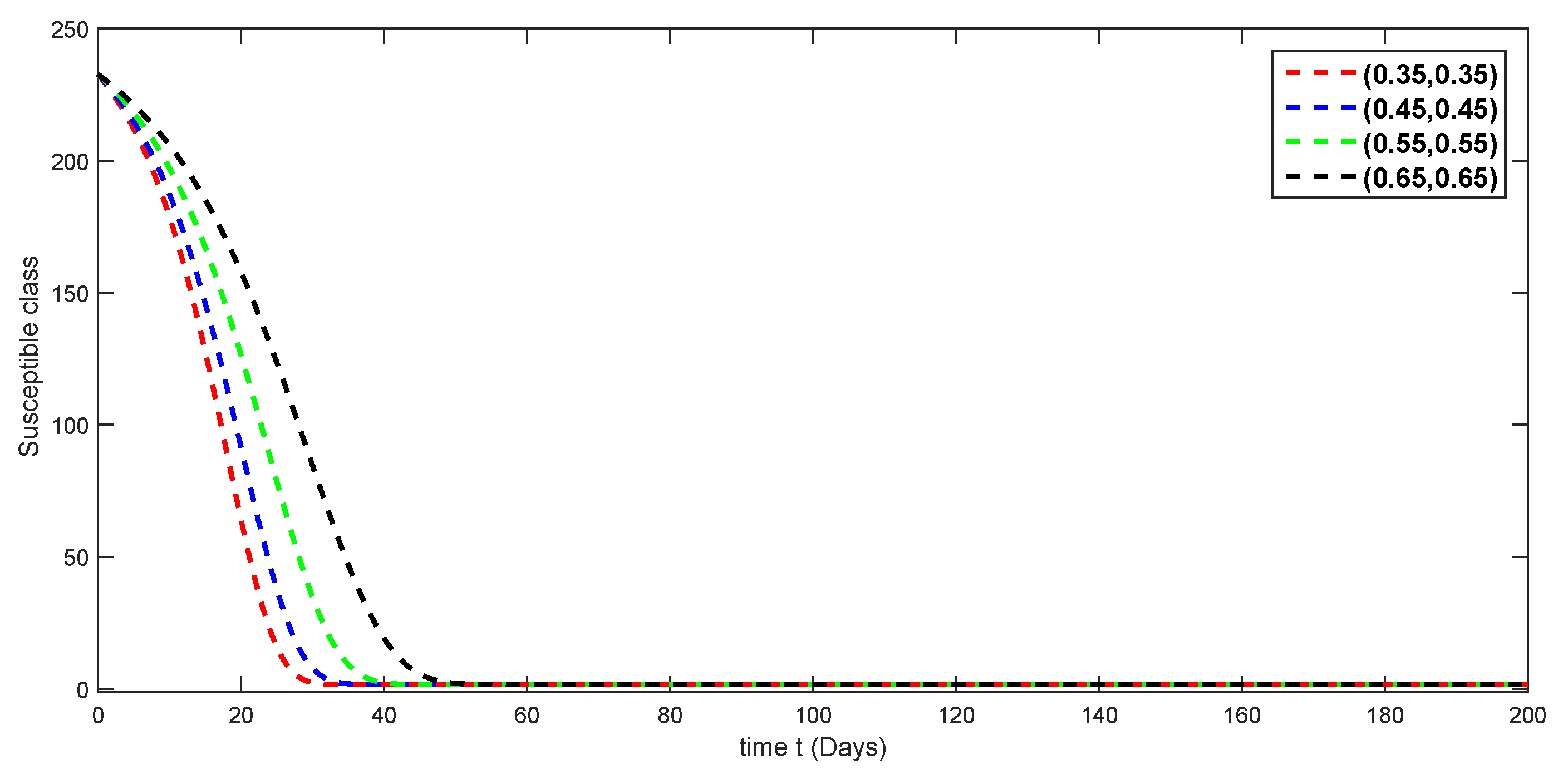
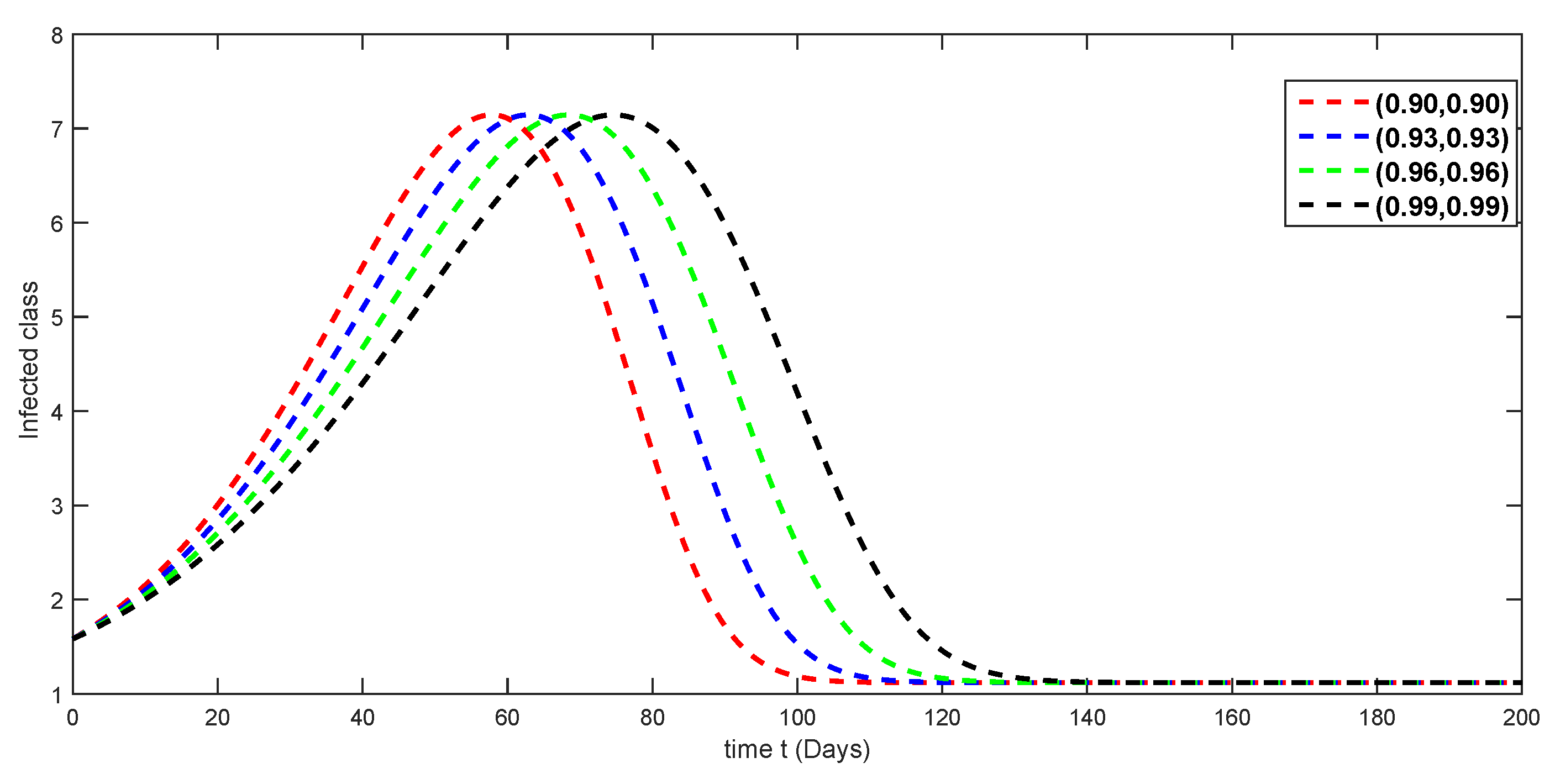
7. Numerical Simulations and Discussion

We have developed a numerical approach to approximate solutions for the fractal-fractional order SIR epidemic model with harmonic mean incidence rate. Our investigation of this model involves exploring different scenarios associated with the fractal-fractional order SIR model with harmonic mean incidence rate. Utilizing the iterative technique mentioned above, we have graphically represented the outcomes of the fractal-fractional SIR model with our suggested incidence rate. To observe the model’s dynamics more effectively, we have selected appropriate constant values for its parameters. Here, we remark that researchers have introduced two important methods to estimate the model parameters from available data. The corresponding two techniques usually used in estimating the parameters are the maximum likelihood and least squares approaches. These two approaches yield parameter estimators with numerous desirable characteristics. Nonetheless, the presence of outliers affects least squares and maximum likelihood calculations equally. It is pertinent to mention that robust methods, a relatively recent class of parameter estimation techniques, have also been deduced. In these techniques, researchers combine the favorable characteristics and efficiency of maximum likelihood and least squares with less vulnerability to outliers. We used the methodology mentioned in [62] to estimate some of the unknown parameters. Here, we use the values in

Table 1. Numerical values of parameters and compartments.

Symbol	Numerical Values	Symbol	Numerical Values
$\upsilon$	$0.00032$ estimated	$\rho$	$0.00018$ estimated
$\mu$	$0.000007$ [63]	$\beta$	$0.00414$ estimated
$\gamma$	$0.98$ [63]	${\gamma }_1$	$0.0018$ estimated
${\gamma }_2$	$0.0029$ estimated	${\mathbf{S}}_0$	$232.648711$ million [63]
${\mathbf{I}}_0$	$1.581936$ million [63]	${\mathbf{R}}_0$	$1.538689$ million [63]

.

We use the available data from Pakistan for 200 days to simulate the results of our model graphically. In Figure 2, we present the population dynamic of the proposed model for three compartments.

Here, in Figure 3, Figure 4 and Figure 5 we present the numerical illustrations for different compartments using various values of fractals and factional orders.

In addition, we simulate the numerical results for slightly larger values of fractals and fractional orders in Figure 6, Figure 7 and Figure 8.

Finally, we interpret the approximate solutions for all three compartments using larger values of fractals and fractional orders in Figure 9, Figure 10 and Figure 11.

We see that the population of the susceptible class decreases with different fractal-fractional orders. In the meantime, the density of the infected class rapidly rises, and then, it goes on decreasing. Also, the population density of the recovered class increases until it becomes stable. Increasing the values of fractal-fractional orders leads to a more pronounced effect on the transmission dynamics of the disease. Furthermore, we also conclude that if $\beta$ in $\frac{2\beta SI}{S+I}$ is small, it indicates a low rate of transmission. In this case, the effective contact rate will also be low, suggesting a slower spread of the disease. If $\beta$ increases, the effective contact rate increases proportionally, leading to a faster spread of the disease. When $\beta$ reaches a certain threshold, the effective contact rate may become high enough to trigger rapid transmission, resulting in a significant increase in the spread of the disease. However, if $\beta$ continues to increase beyond a certain point, it may lead to saturation effects, where the effective contact rate reaches a maximum value, and further increases in $\beta$ do not significantly enhance disease spread. Therefore, for the different values of $\beta$, $\frac{2\beta SI}{S+I}$ allows us to understand how changes in the propagation rate affect the dynamics of disease spread in the SIR model. Intervention strategies, such as travel limitations, vector control efforts, public health messages, social distancing campaigns, vaccination campaigns, quarantine laws, and therapy advancements, greatly influence the dynamics of disease. In the end, these tactics shape the progression and intensity of disease outbreaks by influencing variables such as infection periods, death rates, recovery rates, transmission rates, and vector abundance.

Based on the simulated results above, we conclude that two new techniques in applied mathematics and systems theory, fractal-fractional derivatives and V-L matrices, can represent anomalous diffusion and fractal dynamics and enhance stability analysis for nonlinear systems. Combining these tools offers a powerful approach for modeling systems with both memory and fractal properties. In control theory, this integration can improve the robustness and efficiency of controllers for fractional-order systems, enhancing performance in applications like robotics and aerospace. In biology, it can lead to more accurate models of neural activity and heart rate variability, improving diagnostic tools and treatment strategies. In engineering, health, financial modeling, and environmental science, V-L matrices and fractal-fractional derivatives can be used to improve control systems. In the fields of aerospace, manufacturing, health, and finance, they improve stability, resilience, risk assessment, and trading algorithms.

Some Discussion and Potential Limitations of Our Assumptions and Tools

Here, we remark that the considered model is brief and includes only three classes, which provides an indication for extending it in the future by adding more classes like vaccination, isolation and death classes to obtain more comprehensive results. For the existence theory, we have considered Lipschitz conditions on nonlinear functions. Here, in the future, these can be extended by taking Hölder continuity. Because the said continuity implies uniform continuity. On the other hand, in mathematical biology, the Volterra-type Lyapunov functions are a common tool for determining global stability in systems. But sometimes the formation of such a function is a very tedious job, although the mentioned tools have been used as powerful tools to prove the global asymptotic stability of equilibrium points. The numerical scheme, we used was based on the Adam Bashforth procedure; this has increasingly been used in the last few years to approximate the solutions of many nonlinear problems of fractals and fractional orders. In epidemic models, the mentioned method has been used extensively. However, some limitations of the mentioned tool also exist. For instance, for numerical investigations of oscillatory phenomena, the said tool suffers from instability like the Runge–Kutta method of order four. To overcome this shortcoming, short time intervals should be used.

8. Conclusions

In conclusion, this manuscript explores the application of fractal-fractional derivatives in enhancing our understanding of epidemic dynamics within the context of the $SIR$ model. It introduces the concept of the harmonic mean incidence rate as a modification to the traditional $SIR$ framework, thereby incorporating non-local behaviors into the model. Initially, the model’s global stability is explored utilizing V-L matrix theory. Following this, the groundwork for additional analysis is laid by introducing essential definitions of fractal-fractional derivatives and establishing the required theoretical framework. The subsequent discussion focuses on the modified $SIR$ epidemic model with harmonic mean incidence rate, providing a detailed explanation of its theoretical foundations and presenting findings that provide more insight into the stability and functioning of the system. Further, a numerical scheme is provided, which offers practical insights into executing the model beyond theoretical concepts. Graphical representations of the model’s dynamics are provided to assist researchers in understanding how a disease spreads in different scenarios.

In the future, our main goal is to investigate the application of fractal-fractional derivatives and generalization of the V-L matrix theory to analyze the global stability of various systems, including nonlinear, time-varying, and hybrid systems. It employs linear matrix inequality techniques, providing a robust framework for assessing stability in both linear and nonlinear systems, enhancing its applicability in control theory and dynamical systems.

References

1. Roccetti, M. Drawing a parallel between the trend of confirmed COVID-19 deaths in the winters of 2022/2023 and 2023/2024 in Italy, with a prediction. Math. Biosci. Eng. 2024, 21, 3742–3754. [Google Scholar] [CrossRef] [PubMed]
2. Mohamadou, Y.; Halidou, A.; Kapen, P.T. A review of mathematical modeling, artificial intelligence and datasets used in the study, prediction and management of COVID-19. Appl. Intell. 2020, 50, 3913–3925. [Google Scholar] [CrossRef] [PubMed]
3. Margenov, S.; Popivanov, N.; Ugrinova, I.; Hristov, T. Mathematical Modeling and Short-Term Forecasting of the COVID-19 Epidemic in Bulgaria: SEIRS Model with Vaccination. Mathematics 2022, 10, 2570. [Google Scholar] [CrossRef]
4. Vytla, V.; Ramakuri, S.K.; Peddi, A.; Srinivas, K.K.; Ragav, N.N. Mathematical models for predicting COVID-19 pandemic: A review. J. Phys. Conf. Ser. 2021, 1797, 012009. [Google Scholar] [CrossRef]
5. Starshinova, A.; Osipov, N.; Dovgalyk, I.; Kulpina, A.; Belyaeva, E.; Kudlay, D. COVID-19 and Tuberculosis: Mathematical Modeling of Infection Spread Taking into Account Reduced Screening. Diagnostics 2024, 14, 698. [Google Scholar] [CrossRef] [PubMed]
6. Ma, Y.; Liu, J.B.; Li, H. Global dynamics of an SIQR model with vaccination and elimination hybrid strategies. Mathematics 2018, 6, 328. [Google Scholar] [CrossRef]
7. Upadhyay, R.K.; Pal, A.K.; Kumari, S.; Roy, P. Dynamics of an SEIR epidemic model with nonlinear incidence and treatment rates. Nonlinear Dyn. 2019, 96, 2351–2368. [Google Scholar] [CrossRef]
8. Mwasa, A.; Tchuenche, J.M. Mathematical analysis of a cholera model with public health interventions. Biosystems 2011, 105, 190–200. [Google Scholar] [CrossRef]
9. Wang, L.; Xu, R. Global stability of an SEIR epidemic model with vaccination. Int. J. Biomath. 2016, 9, 1650082. [Google Scholar] [CrossRef]
10. Bentaleb, D.; Amine, S. Lyapunov function and global stability for a two-strain SEIR model with bilinear and non-monotone incidence. Int. J. Biomath. 2019, 12, 1950021. [Google Scholar] [CrossRef]
11. Chen, X.; Cao, J.; Park, J.H.; Qiu, J. Stability analysis and estimation of domain of attraction for the endemic equilibrium of an SEIQ epidemic model. Nonlinear Dyn. 2017, 87, 975–985. [Google Scholar] [CrossRef]
12. Baba, I.A.; Hincal, E. Global stability analysis of two-strain epidemic model with bilinear and non-monotone incidence rates. Eur. Phys. J. Plus 2017, 132, 208. [Google Scholar] [CrossRef]
13. Geng, Y.; Xu, J. Stability preserving NSFD scheme for a multi-group SVIR epidemic model. Math. Methods Appl. Sci. 2017, 40, 4917–4927. [Google Scholar] [CrossRef]
14. McCluskey, C.C. Global stability for an SIR epidemic model with delay and nonlinear incidence. Nonlinear Anal. Real World Appl. 2010, 11, 3106–3109. [Google Scholar] [CrossRef]
15. Arfan, M.; Shah, K.; Ullah, A. Fractal-fractional mathematical model of four species comprising of prey-predation. Phys. Scr. 2021, 96, 124053. [Google Scholar] [CrossRef]
16. Wang, X.; Liu, X.; Xie, W.C.; Xu, W.; Xu, Y. Global stability and persistence of HIV models with switching parameters and pulse control. Math. Comput. Simul. 2016, 123, 53–67. [Google Scholar] [CrossRef]
17. Hu, Z.; Ma, W.; Ruan, S. Analysis of SIR epidemic models with nonlinear incidence rate and treatment. Math. Biosci. 2012, 238, 12–20. [Google Scholar] [CrossRef] [PubMed]
18. Misra, A.K.; Sharma, A.; Shukla, J.B. Stability analysis and optimal control of an epidemic model with awareness programs by media. Biosystems 2015, 138, 53–62. [Google Scholar] [CrossRef] [PubMed]
19. Thieme, H.R. Global stability of the endemic equilibrium in infinite dimension: Lyapunov functions and positive operators. J. Diff. Equ. 2011, 250, 3772–3801. [Google Scholar] [CrossRef]
20. Naik, P.A.; Farman, M.; Zehra, A.; Nisar, K.S.; Hincal, E. Analysis and modeling with fractal-fractional operator for an epidemic model with reference to COVID-19 modeling. Partial Differ. Equ. Appl. Math. 2024, 10, 100663. [Google Scholar] [CrossRef]
21. Shah, K.; Sarwar, M.; Abdeljawad, T. On mathematical model of infectious disease by using fractals fractional analysis. Discret. Contin. Dyn. Syst.—S 2024. [Google Scholar] [CrossRef]
22. Kubra, K.T.; Ali, R.; Alqahtani, R.T.; Gulshan, S.; Iqbal, Z. Analysis and comparative study of a deterministic mathematical model of SARS-COV-2 with fractal-fractional operators: A case study. Sci. Rep. 2024, 14, 6431. [Google Scholar] [CrossRef] [PubMed]
23. Farman, M.; Akgül, A.; Hashemi, M.S.; Guran, L.; Bucur, A. Fractal fractional order operators in computational techniques for mathematical models in epidemiology. Comput. Model. Eng. Sci. 2024, 138, 1385–1402. [Google Scholar] [CrossRef]
24. Fowler, A.C. Mathematical Models in the Applied Sciences; Cambridge University Press: Cambridge, UK, 1997; Volume 17. [Google Scholar]
25. West, B.J. Fractal physiology and the fractional calculus: A perspective. Front. Physiol. 2010, 1, 1886. [Google Scholar] [CrossRef] [PubMed]
26. Baishya, C.; Achar, S.J.; Veeresha, P. An Application of the Caputo Fractional Domain in the Analysis of a COVID-19 Mathematical Model. Contemp. Math. 2024, 5, 255–283. [Google Scholar] [CrossRef]
27. Gao, W.; Veeresha, P.; Cattani, C.; Baishya, C.; Baskonus, H.M. Modified predictor-corrector method for the numerical solution of a fractional-order SIR model with 2019-nCoV. Fractal Fract. 2022, 6, 92. [Google Scholar] [CrossRef]
28. Achar, S.J.; Baishya, C.; Veeresha, P.; Akinyemi, L. Dynamics of fractional model of biological pest control in tea plants with Beddington-DeAngelis functional response. Fractal Fract. 2021, 6, 1. [Google Scholar] [CrossRef]
29. Jan, R.; Khan, A.; Boulaaras, S.; Ahmed Zubair, S. Dynamical behaviour and chaotic phenomena of HIV infection through fractional calculus. Discret. Dyn. Nat. Soc. 2022, 2022, 5937420. [Google Scholar] [CrossRef]
30. Tang, T.Q.; Jan, R.; Bonyah, E.; Shah, Z.; Alzahrani, E. Qualitative analysis of the transmission dynamics of dengue with the effect of memory, reinfection, and vaccination. Comput. Math. Methods Med. 2022, 2022, 7893570. [Google Scholar] [CrossRef] [PubMed]
31. Jan, R.; Boulaaras, S.; Shah, S.A.A. Fractional-calculus analysis of human immunodeficiency virus and CD4+ T-cells with control interventions. Commun. Theor. Phys. 2022, 74, 105001. [Google Scholar] [CrossRef]
32. Jan, A.; Boulaaras, S.; Abdullah, F.A.; Jan, R. Dynamical analysis, infections in plants, and preventive policies utilizing the theory of fractional calculus. Eur. Phys. J. Spec. Top. 2023, 232, 2497–2512. [Google Scholar] [CrossRef]
33. Shah, Z.; Bonyah, E.; Alzahrani, E.; Jan, R.; Alreshidi, N.A. Chaotic phenomena and oscillations in dynamical behaviour of financial system via fractional calculus. Complexity 2022, 2022, 8113760. [Google Scholar] [CrossRef]
34. Jan, R.; Boulaaras, S.; Alyobi, S.; Jawad, M. Transmission dynamics of Hand-Foot-Mouth Disease with partial immunity through non-integer derivative. Int. J. Biomath. 2023, 16, 2250115. [Google Scholar] [CrossRef]
35. Jan, R.; Khan, H.; Kumam, P.; Tchier, F.; Shah, R.; Jebreen, H.B. The investigation of the fractional-view dynamics of Helmholtz equations within Caputo operator. Comput. Mater. Contin. 2021, 68, 3185–3201. [Google Scholar] [CrossRef]
36. Jan, R.; Razak, N.N.A.; Boulaaras, S.; Rehman, Z.U.; Bahramand, S. Mathematical analysis of the transmission dynamics of viral infection with effective control policies via fractional derivative. Nonlinear Eng. 2023, 12, 20220342. [Google Scholar] [CrossRef]
37. Jódar, L.; Villanueva, R.J.; Arenas, A.J.; González, G.C. Nonstandard numerical methods for a mathematical model for influenza disease. Math. Comput. Simul. 2008, 79, 622–633. [Google Scholar] [CrossRef]
38. Khan, A.; Abdeljawad, T.; Alqudah, M.A. Neural networking study of worms in a wireless sensor model in the sense of fractal fractional. AIMS Math. 2023, 8, 26406–26424. [Google Scholar] [CrossRef]
39. Shah, K.; Abdeljawad, T. On complex fractal-fractional order mathematical modeling of CO2 emanations from energy sector. Phys. Scr. 2023, 99, 015226. [Google Scholar] [CrossRef]
40. Shafiullah; Shah, K.; Sarwar, M.; Abdeljawad, T. On theoretical and numerical analysis of fractal–fractional non-linear hybrid differential equations. Nonlinear Eng. 2024, 13, 20220372. [Google Scholar] [CrossRef]
41. Shah, K.; Arfan, M.; Mahariq, I.; Ahmadian, A.; Salahshour, S.; Ferrara, M. Fractal-fractional mathematical model addressing the situation of corona virus in Pakistan. Results Phys. 2020, 19, 103560. [Google Scholar] [CrossRef]
42. Khan, Z.A.; Shah, K.; Abdalla, B.; Abdeljawad, T. A numerical study of complex dynamics of a chemostat model under fractal-fractional derivative. Fractals 2023, 31, 2340181. [Google Scholar] [CrossRef]
43. Strichartz, R.S. Analysis on fractals. Not. AMS 1999, 46, 1199–1208. [Google Scholar]
44. Dietz, K. The estimation of the basic reproduction number for infectious diseases. Stat. Methods Med Res. 1993, 2, 23–41. [Google Scholar] [CrossRef] [PubMed]
45. Chien, F.; Shateyi, S. Volterra-Lyapunov stability analysis of the solutions of babesiosis disease model. Symmetry 2021, 13, 1272. [Google Scholar] [CrossRef]
46. Zahedi, M.S.; Kargar, N.S. The Volterra-Lyapunov matrix theory for global stability analysis of a model of HIV/AIDS. Int. J. Biomath. 2017, 10, 1750002. [Google Scholar] [CrossRef]
47. Shao, P.; Shateyi, S. Stability Analysis of SEIRS Epidemic Model with Nonlinear Incidence Rate Function. Mathematics 2021, 9, 2644. [Google Scholar] [CrossRef]
48. Masoumnezhad, M.; Rajabi, M.; Chapnevis, A.; Dorofeev, A.; Shateyi, S.; Kargar, N.S.; Nik, H.S. An approach for the global stability of mathematical model of an infectious disease. Symmetry 2020, 12, 1778. [Google Scholar] [CrossRef]
49. Atangana, A.; Gómez-Aguilar, J.F. Numerical approximation of Riemann-Liouville definition of fractional derivative: From Riemann-Liouville to Atangana-Baleanu. Numer. Methods Partial Differ. Equ. 2018, 34, 1502–1523. [Google Scholar] [CrossRef]
50. Atangana, A. Fractal-fractional differentiation and integration: Connecting fractal calculus and fractional calculus to predict complex system. Chaos Solitons Fractals 2017, 102, 396–406. [Google Scholar] [CrossRef]
51. Ahmad, S.; Shah, K.; Abdeljawad, T.; Abdalla, B. On the Approximation of Fractal-Fractional Differential Equations Using Numerical Inverse Laplace Transform Methods. Comput. Model. Eng. Sci. 2023, 135, 2743. [Google Scholar]
52. Ali, Z.; Rabiei, F.; Shah, K.; Khodadadi, T. Fractal-fractional order dynamical behavior of an HIV/AIDS epidemic mathematical model. Eur. Phys. J. Plus 2021, 136, 36. [Google Scholar] [CrossRef]
53. Khan, Z.A.; Rahman, M.U.; Shah, K. Study of a fractal-fractional smoking models with relapse and harmonic mean type incidence rate. J. Funct. Spaces 2021, 2021, 6344079. [Google Scholar] [CrossRef]
54. Abdel-Gawad, H.I.; Baleanu, D.; Abdel-Gawad, A.H. Unification of the different fractional time derivatives: An application to the epidemic-antivirus dynamical system in computer networks. Chaos Solitons Fractals 2021, 142, 110416. [Google Scholar] [CrossRef]
55. Singh, J.; Kumar, D.; Hammouch, Z.; Atangana, A. A fractional epidemiological model for computer viruses pertaining to a new fractional derivative. Appl. Math. Comput. 2018, 316, 504–515. [Google Scholar] [CrossRef]
56. Özdemir, N.; Uçar, S.; Iskender Eroglu, B.B. Dynamical analysis of fractional order model for computer virus propagation with kill signals. Int. J. Nonlinear Sci. Numer. Simul. 2020, 21, 239–247. [Google Scholar] [CrossRef]
57. Kumar, D.; Singh, J. New aspects of fractional epidemiological model for computer viruses with Mittag-Leffler law. In Mathematical Modelling in Health, Social and Applied Sciences; Springer: Singapore, 2020; pp. 283–301. [Google Scholar]
58. Maji, C.; Al Basir, F.; Mukherjee, D.; Ravichandran, C.; Nisar, K. COVID-19 propagation and the usefulness of awareness-based control measures: A mathematical model with delay. AIMs Math. 2022, 7, 12091–12105. [Google Scholar] [CrossRef]
59. Perko, L. Differential Equations and Dynamical Systems; Springer Science & Business Media: Berlin/Heidelberg, Germany, 2013; Volume 7. [Google Scholar]
60. Strogatz, S.H. Nonlinear Dynamics and Chaos: With Applications to Physics, Biology, Chemistry, and Engineering; CRC Press: Boca Raton, FL, USA, 2018. [Google Scholar]
61. Yusuf, T.T. On global stability of disease-free equilibrium in epidemiological models. Eur. J. Math. Stat. 2021, 2, 37–42. [Google Scholar] [CrossRef]
62. Johnson, M.L.; Faunt, L.M. Parameter estimation by least-squares methods, In Methods in Enzymology; Academic Press: New York, NY, USA, 1992; Volume 210, pp. 1–37. [Google Scholar]
63. Worldometer. Available online: https://www.worldometers.info/coronavirus/country/pakistan/ (accessed on 12 March 2024).
Figure 1. Schematic diagram of model (20).
Fractalfract 08 00321 g001
Figure 2. Population dynamic for using ε = δ = 1 .
Fractalfract 08 00321 g002
Figure 3. Interpretation of susceptible class for using various values of ε , δ ( 0 , 0.65 ] .
Fractalfract 08 00321 g003
Figure 4. Interpretation of infected class for using various values of ε , δ ( 0 , 0.65 ] .
Fractalfract 08 00321 g004
Figure 5. Interpretation of recovered class for using various values of ε , δ ( 0 , 0.65 ] .
Fractalfract 08 00321 g005
Figure 6. Interpretation of susceptible class for using various values of ε , δ [ 0.70 , 0.65 ] .
Fractalfract 08 00321 g006
Figure 7. Interpretation of infected class for using various values of ε , δ [ 0.70 , 0.65 ] .
Fractalfract 08 00321 g007
Figure 8. Interpretation of recovered class for using various values of ε , δ [ 0.70 , 0.65 ] .
Fractalfract 08 00321 g008
Figure 9. Interpretation of susceptible class for using various values of ε , δ [ 0.90 , 0.99 ] .
Fractalfract 08 00321 g009
Figure 10. Interpretation of infected class for using various values of ε , δ [ 0.90 , 0.99 ] .
Fractalfract 08 00321 g010
Figure 11. Interpretation of recovered class for using various values of ε , δ [ 0.90 , 0.99 ] .
Fractalfract 08 00321 g011