Exploring Novel Soliton Solutions to the Time-Fractional Coupled Drinfel’d–Sokolov–Wilson Equation in Industrial Engineering Using Two Efficient Techniques

Abstract

The time-fractional coupled Drinfel’d–Sokolov–Wilson (DSW) equation is pivotal in soliton theory, especially for water wave mechanics. Its precise description of soliton phenomena in dispersive water waves makes it widely applicable in fluid dynamics and related fields like tsunami prediction, mathematical physics, and plasma physics. In this study, we present novel soliton solutions for the DSW equation, which significantly enhance the accuracy of describing soliton phenomena. To achieve these results, we employed two distinct methods to derive the solutions: the Sardar subequation method, which works with one variable, and the $\left(\frac{{\mathsf{\Omega }}^{\prime }}{\mathsf{\Omega }}, \frac{1}{\mathsf{\Omega }}\right)$ method which utilizes two variables. These approaches supply significant improvements in efficiency, accuracy, and the ability to explore a broader spectrum of soliton solutions compared to traditional computational methods. By using these techniques, we construct a wide range of wave structures, including rational, trigonometric, and hyperbolic functions. Rigorous validation with Mathematica software 13.1 ensures precision, while dynamic visual representations illustrate soliton solutions with diverse patterns such as dark solitons, multiple dark solitons, singular solitons, multiple singular solitons, kink solitons, bright solitons, and bell-shaped patterns. These findings highlight the effectiveness of these methods in discovering new soliton solutions and supplying deeper insights into the DSW model’s behavior. The novel soliton solutions obtained in this study significantly enhance our understanding of the DSW equation’s underlying dynamics and offer potential applications across various scientific fields.

1. Introduction

Nonlinear equations (NLEs) serve as the cornerstone of scientific inquiry and technological advancement, enabling the depiction of complex systems and phenomena that elude linear models. Their application spans numerous disciplines, from physics, mathematics, and engineering to biology and economics, owing to their unmatched ability to capture real-world complexities such as fluid dynamics and population dynamics [1,2,3,4]. Moreover, nonlinear systems often unveil emergent behaviors, giving rise to intricate patterns and structures from simple interactions, underscoring the need to explore their dynamics comprehensively. In essence, nonlinear equations are indispensable tools for unraveling nature’s complexities, driving innovation, and expanding scientific horizons. Furthermore, fractional nonlinear differential equations (FNLDEs) serve as robust mathematical tools for modeling diverse physical phenomena, accounting for long-range interactions and non-local effects through fractional-order partial derivatives. Their applications span various fields including fluid mechanics, optical physics, finance, plasma physics, biology, and many others. Unlike classical NLEs, FNLDEs pose challenges in solving due to their non-local nature [5,6]. Nevertheless, researchers employ fractional models to find exact solutions because they more precisely represent complex systems with memory and hereditary properties. These models are especially advantageous in fields such as viscoelasticity, anomalous diffusion, and financial markets, where historical states influence current behavior. By extending classical models through fractional calculus, fractional models capture nuances that integer-order models miss, producing solutions that closely match real-world data. This greater accuracy and flexibility make fractional models vital for understanding and predicting the behavior of intricate systems across various scientific and engineering disciplines [7,8]. Among various NLEs, the conformable time fractional coupled DSW equations were developed, stemming from shallow-water wave models, originating from the work of Drinfel’d and Sokolov, with further advancements by Wilson. The DSW equations, based on the diffusive wave approximation of shallow-water equations, find successful applications in modeling various phenomena such as wave overtopping, floods, dam breaks, and flows through vegetated areas, primarily driven by gravitational forces and dominated by shear stress [9,10]. Additionally, they blend conformable fractional calculus and time-fractional derivatives, offering a framework for analyzing nonlinear wave propagation with memory effects. By scrutinizing its traveling wave solutions, researchers glean insights into various wave dynamics, including shape, speed, and stability during propagation. This understanding proves vital for comprehending phenomena like soliton propagation, wave interactions, and pattern formation. With applications spanning fields such as nonlinear optics, fluid dynamics, and mathematical biology, where fractional-order dynamics prevail, the coupled time-fractional DSW equations hold significant relevance and potential for further exploration. By comprehensively studying traveling wave propagation within the DSW equation, we gain valuable insights into their behavior across these systems, thereby deepening our understanding of their dynamics. The DSW equations, with fractional derivative concerning time, are given as follows [6,11]:

$$\left.\begin{array}{c}{D}_t^{\alpha }\left({\mathbb{Q}}_t\right)+\beta \mho {\mho }_x=0\\ D_t^{\alpha }\left({\mho }_t\right)+\varrho \mathbb{Q}{\mho }_x+{\delta \mathbb{Q}}_x\mho +\sigma {\mho }_{xxx}=0\end{array}\right\},$$

(1)

where $\mathbb{Q}=\mathbb{Q}(x,t)$ and $\mho =\mho (x,t)$ represent the functions of time and space, $\alpha$ is the fractional order, and $\beta$, $\gamma$, $\delta$, and $\sigma$ are all non-zero constants.

Given the substantial interest and importance placed on obtaining exact solutions for NLEs, numerous researchers have endeavored to employ a diverse array of mathematical techniques to achieve this objective. These techniques encompass a wide spectrum of methodologies, including the modified simple equation method [12], the generalized $\left(G^{\prime }/G\right)$-expansion technique [13], the ($\frac{G^{\prime }}{G^{\prime }+G+A})$ technique [14], the Hirota bilinear method [15], the Riccati equation technique [16], the Lie group approach [17], the extended Jacobi elliptic function approach [18], the exp $\left\{-\phi \left(\xi \right)\right\}$ method [19], the functional variable technique [20], the multiple exp-function technique [21], the new auxiliary equation technique [22], the tanh-function approach [23], the simple equation technique [24], the tanh–coth technique [25], the generalized Kudryshov technique [26], the unified technique [27], and so on.

Given the considerable significance of the DSW equations across scientific disciplines, numerous researchers have dedicated efforts to uncover solutions. For instance, Santillana and Dawson (2009) explored the soliton solution of the DSW equations by employing the Galerkin finite element approach [28], while truncated Painlevé and Mobius invariant forms were utilized for obtaining explicit solutions featuring non-local symmetry, as detailed in [29]. The F-expansion technique was used to find the exact solutions to DSW equations, as outlined in reference [30]. Furthermore, Sahoo and Ray (2017) employed the Jacobi elliptic function approach to derive double-periodic solutions [31]. Utilizing the Adomian decomposition approach, [32] applied it to approximate doubly periodic wave solutions of classical DSW equations. Nonetheless, finding exact solutions for the time-fractional DSW system poses greater challenges compared to standard DSW equations. While most studies concentrate on the latter, the focus on fractional DSW equations is yet in its early stages. In this context, this study concentrated on obtaining novel soliton solutions for the fractional DSW equation using the most appropriate methods.

Among various methods, the Sardar subequation method stands out as a potent analytical technique for solving NLEs. This method represents solutions as power series, with coefficients determined by a single variable. By substituting these series into the equation and equating coefficients of similar terms, the method systematically derives these coefficients. This method has proven effective in revealing analytical solutions for various NLEs [33,34,35,36,37,38]. In addition, the $\left(\frac{{\mathsf{\Omega }}^{\prime }}{\mathsf{\Omega }}, \frac{1}{\mathsf{\Omega }}\right)$ expansion method is an influential analytical approach used for tackling NLEs. It involves expressing solutions as power series, with coefficients determined through two variables ($\frac{{\mathsf{\Omega }}^{\prime }}{\mathsf{\Omega }}$ and $\frac{1}{\mathsf{\Omega }}$). These coefficients are achieved by replacing the series keen on the equation and aligning coefficients of similar terms. Due to its effectiveness, numerous researchers [39,40,41,42,43,44,45] have utilized this technique to reveal solutions for various NLEs. As of present, there has been no investigation into Equation (1) using these specific methods. This study aims to derive precise solutions for the supplied nonlinear equation employing the designated methodologies. The manuscript is structured as follows: (i) Section 2 supplies an overview of fractional derivatives; (ii) Section 3 presents an overview of the methods used; (iii) In Section 4, these methods are applied to the equation, resulting in the derivation of the requisite solutions; (iv) Section 5 explores dynamic interpretations, illustrating the fascinating behaviors of various soliton solutions across 2D, 3D, and contour graphs, along with discussion; (v) Concluding remarks are offered in Section 6; (vi) Finally, the paper concludes with a comprehensive list of references.

2. Review of Time-Fractional Derivative

A fractional derivative extends differentiation to non-integer orders while adhering to conventional calculus rules. Unlike integer-order derivatives, which apply to functions with integer degrees of differentiability, fractional derivatives enable differentiation at non-integer orders, enhancing the comprehension of function behavior.

Definition 1. 

The time-fractional derivative of a function   $\mathcal{F}\left(t\right)$ with order  $\alpha$ is defined as follows [46]:

$$D_t^{\alpha }\mathcal{F}\left(t\right)=\underset{h\to 0}{\lim }\left\{\frac{\mathcal{F}\left(t+h{t}^{1-\alpha }\right)-\mathcal{F}\left(t\right)}{h}\right\},$$

(2)

where  $t$ is consistently assigned non-negative values, and the derivative’s order remains$0<\alpha \le 1$.

According to [47], the definition above fulfills the requirements of the following proposition.

Proposition 1. 

If  $\alpha$ falls within the interval  $0<\alpha \le 1$, with  $a$, b, and  $\tau$ as real numbers and with  $\mathcal{F}=\mathcal{F}\left(t\right),\mathcal{H}=\mathcal{H}\left(t\right)$ being fractionally differentiable at a given point $t$, then the following characteristics must hold:

• $D_t^{\alpha }\left(a\mathcal{F}+b\mathcal{H}\right)={aD}_t^{\alpha }\mathcal{F}+{bD}_t^{\alpha }\mathcal{H}$;
• $D_t^{\alpha }\left(t^{\tau }\right)=\tau t^{\tau -\alpha }$;
• $D_t^{\alpha }\left(\mathcal{F}\mathcal{H}\right)={\mathcal{F}D}_t^{\alpha }\mathcal{H}+{\mathcal{H}D}_t^{\alpha }\mathcal{F}$;
• $D_t^{\alpha }\left(\mathcal{F}/\mathcal{H}\right)=\frac{{\mathcal{H}D}_t^{\alpha }\mathcal{F}-{\mathcal{F}D}_t^{\alpha }\mathcal{H}}{{\mathcal{H}}^2}$;
• $D_t^{\alpha }\left(\mathcal{F}o\mathcal{H}\right)=t^{1-\alpha }{\mathcal{F}}^{\prime }\left\{\mathcal{H}\left(t\right)\right\}{\mathcal{H}}^{\prime }\left(t\right)$.

Nonetheless,$D_t^{\alpha }\mathcal{F}\left(t\right)=t^{1-\alpha }\frac{d\mathcal{F}}{dt}=t^{1-\alpha }{\mathcal{F}}^{\prime };D_t^{\alpha }\mathcal{H}\left(t\right)=t^{1-\alpha }\frac{d\mathcal{H}}{dt}={t^{1-\alpha }\mathcal{H}}^{\prime }$, where  $\mathcal{F}$ and  $\mathcal{H}$ must be differentiable.

3. Methodology

The Sardar Subequation Approach

In this section, we have discussed the Sardar subequation method, valued for its ability to supply precise solutions for a variety of NLEs. As we have embarked on this analytical journey, we have focused on the typical structure of NLEs, often characterized by three distinct independent variables $x$, $y$, and $t$ as follows:

$$P\left(\mathfrak{R},{\mathfrak{R}}_x,{\mathfrak{R}}_{xx},{\mathfrak{R}}_y,{\mathfrak{R}}_{yy},{\mathfrak{R}}_{xy},{\mathfrak{R}}_t,{\mathfrak{R}}_{tt},{\mathfrak{R}}_{xt},\dots \dots \dots \right)=0,$$

(3)

where $P$ corresponds to a polynomial function with its partial derivatives.

To transform this into an ordinary differential equation (ODE), we introduce a new variable $\psi$, governed by the following relation:

$$\mathbb{Q}\left(x,t\right)=\mathfrak{R}\left(\psi \right),\mho \left(x,t\right)={\rm Y}\left(\psi \right), \mathrm{where} \psi =\left(x-\vartheta \frac{t^{\alpha }}{\alpha }\right)s.$$

(4)

Using Equation (4) in Equation (3), we transform it into an ODE, which takes the following form:

$$J\left(\mathfrak{R},{\mathfrak{R}}^{\prime },{\mathfrak{R}}^{″},{\mathfrak{R}}^{‴},\dots \dots \dots \right)=0,$$

(5)

where the symbol $J$ is a novel polynomial alongside its ordinary derivatives ($\mathfrak{R}=\mathfrak{R}\left(\psi \right),{\mathfrak{R}}^{\mathrm{\prime }}=\frac{d\mathfrak{R}}{d\psi },{\mathfrak{R}}^{\mathrm{″}}=\frac{d^2\mathfrak{R}}{d{\psi }^2},{\mathfrak{R}}^{\mathrm{‴}}=\frac{d^3\mathfrak{R}}{d{\psi }^3},\dots \dots \dots$).

Therefore, Equation (5) supplies the general solution (GS) as follows:

$$\mathfrak{R}\left(\psi \right)={\sum }_{i=0}^N{c}_i{\mathcal{M}}^i\left(\psi \right),$$

(6)

in which

$${\mathcal{M}}^{\prime }\left(\psi \right)=\sqrt{{\mathcal{M}}^4\left(\psi \right)+{\varpi \mathcal{M}}^2\left(\psi \right)+ϵ},$$

(7)

where $c_i$ (i = 1, 2, 3, …, n), $\varpi$ and $ϵ$ are arbitrary constants, and N is the balance number that requires determination.

The solutions derived from Equation (7) are manifested as follows:

Scenario I. 

When $\varpi >0$ but $ϵ=0$, then

$${\mathcal{M}}_1^{\pm }\left(\psi \right)=\pm \sqrt{g\mathcal{l}\varpi } {cosech}_{g\mathcal{l}}\left(\sqrt{\varpi } \psi \right),$$

(8)

$${\mathcal{M}}_2^{\pm }\left(\psi \right)=\pm \sqrt{-g\mathcal{l}\varpi } {sech}_{g\mathcal{l}}\left(\sqrt{\varpi } \psi \right),$$

(9)

where ${cosech}_{g\mathcal{l}}\left(\psi \right)=\frac{2}{g{e}^{\psi }-{\mathcal{l}e}^{-\psi }}$ and ${sech}_{g\mathcal{l}}\left(\psi \right)=\frac{2}{g{e}^{\psi }+{\mathcal{l}e}^{-\psi }}$;

Scenario II. 

When $\varpi <0$ but $ϵ=0$, then

$${\mathcal{M}}_3^{\pm }\left(\psi \right)=\pm \sqrt{-g\mathcal{l}\varpi } {cosec}_{g\mathcal{l}}\left(\sqrt{-\varpi } \psi \right),$$

(10)

$${\mathcal{M}}_4^{\pm }\left(\psi \right)=\pm \sqrt{-g\mathcal{l}\varpi } {sec}_{g\mathcal{l}}\left(\sqrt{-\varpi } \psi \right),$$

(11)

where ${cosec}_{g\mathcal{l}}\left(\psi \right)=\frac{2i}{g{e}^{i\psi }-{\mathcal{l}e}^{-i\psi }}$ and ${sec}_{g\mathcal{l}}\left(\psi \right)=\frac{2}{g{e}^{i\psi }+{\mathcal{l}e}^{-i\psi }}$;

Scenario III. 

When $\varpi <0$ but $ϵ=\frac{{\varpi }^2}{4}$, then

$${\mathcal{M}}_5^{\pm }\left(\psi \right)=\pm \sqrt{-\frac{\varpi }{2}} {tanh}_{g\mathcal{l}}\left(\sqrt{-\frac{\varpi }{2}} \psi \right),$$

(12)

$${\mathcal{M}}_6^{\pm }\left(\psi \right)=\pm \sqrt{-\frac{\varpi }{2}} {coth}_{g\mathcal{l}}\left(\sqrt{-\frac{\varpi }{2}} \psi \right),$$

(13)

$${\mathcal{M}}_7^{\pm }\left(\psi \right)=\pm \sqrt{-\frac{\varpi }{2}} \left\{{tanh}_{g\mathcal{l}}\left(\sqrt{-2\varpi } \psi \right)\pm {i\sqrt{g\mathcal{l}} sech}_{g\mathcal{l}}\left(\sqrt{-2\varpi } \psi \right)\right\},$$

(14)

$${\mathcal{M}}_8^{\pm }\left(\psi \right)=\pm \sqrt{-\frac{\varpi }{2}} \left\{{coth}_{g\mathcal{l}}\left(\sqrt{-2\varpi } \psi \right)\pm {\sqrt{g\mathcal{l}} cosech}_{g\mathcal{l}}\left(\sqrt{-2\varpi } \psi \right)\right\},$$

(15)

$${\mathcal{M}}_9^{\pm }\left(\psi \right)=\pm \sqrt{-\frac{\varpi }{8}} \left\{{tanh}_{g\mathcal{l}}\left(\sqrt{-\frac{\varpi }{8}} \psi \right)+{coth}_{g\mathcal{l}}\left(\sqrt{-\frac{\varpi }{8}} \psi \right)\right\},$$

(16)

where ${tanh}_{g\mathcal{l}}\left(\psi \right)=\frac{g{e}^{\psi }-{\mathcal{l}e}^{-\psi }}{g{e}^{\psi }+{\mathcal{l}e}^{-\psi }}$ and ${coth}_{g\mathcal{l}}\left(\psi \right)=\frac{g{e}^{\psi }+{\mathcal{l}e}^{-\psi }}{g{e}^{\psi }-{\mathcal{l}e}^{-\psi }}$;

Scenario IV. 

When $\varpi >0$ but $ϵ=\frac{{\varpi }^2}{4}$, then

$${\mathcal{M}}_{10}^{\pm }\left(\psi \right)=\pm \sqrt{\frac{\varpi }{2}} {tan}_{g\mathcal{l}}\left(\sqrt{\frac{\varpi }{2}} \psi \right),$$

(17)

$${\mathcal{M}}_{11}^{\pm }\left(\psi \right)=\pm \sqrt{\frac{\varpi }{2}} {cot}_{g\mathcal{l}}\left(\sqrt{\frac{\varpi }{2}} \psi \right),$$

(18)

$${\mathcal{M}}_{12}^{\pm }\left(\psi \right)=\pm \sqrt{\frac{\varpi }{2}} \left\{{tan}_{g\mathcal{l}}\left(\sqrt{2\varpi } \psi \right)\pm {\sqrt{g\mathcal{l}} sec}_{\rho \mathcal{l}}\left(\sqrt{2\varpi } \psi \right)\right\},$$

(19)

$${\mathcal{M}}_{13}^{\pm }\left(\psi \right)=\pm \sqrt{\frac{\varpi }{2}} \left\{{cot}_{g\mathcal{l}}\left(\sqrt{2\varpi } \psi \right)\pm {\sqrt{g\mathcal{l}} cosec}_{g\mathcal{l}}\left(\sqrt{2\varpi } \psi \right)\right\},$$

(20)

$${\mathcal{M}}_{14}^{\pm }\left(\psi \right)=\pm \sqrt{\frac{\varpi }{8}} \left\{{tan}_{g\mathcal{l}}\left(\sqrt{\frac{\varpi }{8}} \psi \right)+{cot}_{g\mathcal{l}}\left(\sqrt{\frac{\varpi }{8}} \psi \right)\right\},$$

(21)

where ${tan}_{g\mathcal{l}}\left(\psi \right)=-i\frac{g{e}^{i\psi }-{\mathcal{l}e}^{-i\psi }}{g{e}^{i\psi }+{\mathcal{l}e}^{-i\psi }}$ and ${cot}_{g\mathcal{l}}\left(\psi \right)=i\frac{g{e}^{i\psi }+{\mathcal{l}e}^{-i\psi }}{g{e}^{i\psi }-{\mathcal{l}e}^{-i\psi }}$.

4. Method Workflow

First, to find the balance number N, we employ the homogeneous balance method. Then, substituting the value of N into Equation (6), we incorporate this modified equation into Equation (5) using Equation (7). This transforms the left-hand side of Equation (5) into a polynomial. Setting the coefficients of matching power terms to zero establishes a system of algebraic equations involving $\varpi$, $ϵ$, and $c_i$. Solving these systems allows us to determine the unknown coefficients, denoted as $c_i$. Substituting these coefficients into Equation (5) provides exact solutions for Equation (1) in the 14 different forms described in the preceding section.

The $\left(\frac{{\Omega }^{\prime }}{\Omega }, \frac{1}{\Omega }\right)$-Expansion Approach

Here, we offer an in-depth guide to utilizing the $\left(\frac{{\mathsf{\Omega }}^{\prime }}{\mathsf{\Omega }}, \frac{1}{\mathsf{\Omega }}\right)$-expansion method. To solve the NLEs presented in Equation (3), we employ the transformation variable specified in Equation (4). This transformation aids in converting the NLEs into ODEs, streamlining the analytical process. Enabling this analytical journey involves crafting an auxiliary linear ODE, depicted as follows:

$${\mathsf{\Omega }}^{″}\left(\psi \right)+\lambda \mathsf{\Omega }\left(\psi \right)=\eta ,$$

(22)

where the variables are expressed as follows:

$$\mathsf{\Pi }\left(\psi \right)=\frac{{\mathsf{\Omega }}^{\prime }\left(\psi \right)}{\mathsf{\Omega }\left(\psi \right)}, \mathrm{and} \mathcal{L}\left(\psi \right)=\frac{1}{\mathsf{\Omega }\left(\psi \right)},$$

(23)

where

$${\mathsf{\Pi }}^{\prime }={-\mathsf{\Pi }}^2+\eta \mathcal{L}-\lambda , \mathrm{and} {\mathcal{L}}^{\prime }=-\mathsf{\Pi }\ast \mathcal{L}.$$

(24)

The solution of Equation (22) varies based on the value of λ, which is categorized as follows:

Case I. 

Trigonometric solutions

$$\mathsf{\Omega }\left(\psi \right)=d_{1}sin\left(\psi \sqrt{\lambda }\right)+d_{2}cos\left(\psi \sqrt{\lambda }\right)+\raisebox{1ex}{$\eta $}\!\left/ \!\raisebox{-1ex}{$\lambda $}\right., \mathrm{when} \lambda >0,$$

(25)

which generates ${\mathcal{L}}^2=\left(\frac{{\mathsf{\Pi }}^2-2\eta \mathcal{L}+\lambda }{{A_1\lambda }^2-{\eta }^2}\right)\lambda$, where $A_1=d_1^2+d_2^2$ is the arbitrary constant;

Case II. 

Hyperbolic solutions

$$\mathsf{\Omega }\left(\psi \right)=d_{1}sinh\left(\psi \sqrt{-\lambda }\right)+d_{2}cosh\left(\psi \sqrt{-\lambda }\right)+\raisebox{1ex}{$\eta $}\!\left/ \!\raisebox{-1ex}{$\lambda $}\right., \mathrm{when} \lambda <0,$$

(26)

which produces ${\mathcal{L}}^2=-\lambda \left(\frac{{\mathsf{\Pi }}^2-2\eta \mathcal{L}+\lambda }{{A_2\lambda }^2+{\eta }^2}\right)$, where $A_2=d_1^2-d_2^2$ is an arbitrary constant;

Case III. 

Rational solutions

$$\mathsf{\Omega }\left(\psi \right)=\frac{\eta {\psi }^2}{2}+d_1\psi +d_2, \mathrm{when} \lambda =0,$$

(27)

which gives ${\mathcal{L}}^2=\left(\frac{{\mathsf{\Pi }}^2-2\eta \mathcal{L}}{d_1^2-2\eta d_2}\right)$.

Thus, Equation (5) has solutions of the following form:

$$\mathfrak{R}\left(\psi \right)=a_0+{\sum }_{j=1}^P{a}_j{\Pi }^j\left(\psi \right)+{\sum }_{j=1}^P{b}_j{\Pi }^{j-1}\left(\psi \right)\mathcal{L}\left(\psi \right).$$

(28)

where $a_0$, $a_j$, and $b_j$ (j = 1, 2, 3,…, P) denote arbitrary constants, ensuring that $a_P^2+b_P^2\ne 0$, and $P$ signifies a positive balance number.

5. Method Roadmap

Initially, we employ the homogeneous balance method to derive the parameter $P$. Once $P$ is determined, it is substituted into Equation (28). Then, Equation (5), along with Equations (23) and (24), is used for further substitution. This process results in a polynomial on the left-hand side of Equation (28), incorporating terms $\Pi$ and $\mathcal{L}$. By setting the coefficients of terms with corresponding powers within the polynomial to 0, a system of algebraic equations is formulated. These equations involve parameters such as $a_0$, $a_j$, $b_j$, $\lambda$, and $\eta$, among others. Solving these algebraic equations yields the values of the parameters. Subsequently, these parameter values are substituted into Equation (28), enabling the extraction of soliton solutions to Equation (1) expressed in trigonometric functions (as in Equation (25)), hyperbolic functions (as in Equation (26)), and rational functions (as in Equation (27)).

5.1. Application

In this section, we employ the coupled fractional derivative along with the methods described in Section 2 and Section 3 to obtain the exact solution to Equation (1).

Applying the transformation outlined in Equation (4) to Equation (1) provides

$$\left.\begin{array}{c}-{s\vartheta \mathfrak{R}}^{\prime }+s\beta {{\rm Y}{\rm Y}}^{\prime }=0\\ -{s\vartheta {\rm Y}}^{\prime }+s\varrho R{{\rm Y}}^{\prime }+s\delta {\mathfrak{R}}^{\prime }{\rm Y}+s^3\sigma {{\rm Y}}^{‴}=0\end{array}\right\}.$$

(29)

Starting from the first equation of the system, we can express $\mathfrak{R}$ in terms of ${\rm Y}$ as follows:

$$\mathfrak{R}=\frac{\beta }{2\vartheta }{{\rm Y}}^2.$$

(30)

Substituting Equation (30) into the second equation in Equation (29), we obtain a transform ODE as follows:

$$-6{\vartheta }^2{\rm Y}+\beta \left(\varrho +2\delta \right){{\rm Y}}^3+6\sigma \vartheta s^2{{\rm Y}}^{″}=0.$$

(31)

Next, we proceed to solve this equation using the method outlined in the preceding sections.

5.2. For the Sardar Subequation Method

Applying the balancing principle to Equation (31), the balance number $N=1$ is found; therefore, the solution takes on the following form:

$${\rm Y}\left(\psi \right)=c_0+c_1\mathcal{M}\left(\psi \right).$$

(32)

Inserting this into Equation (31) yields a series of algebraic equations (see Appendix A). Solving these equations provides the values of the coefficients as follows:

$$c_0=0, c_1=\pm \frac{2\sqrt{3}{s}^2\sigma \sqrt{\varpi }}{\sqrt{-2\delta \beta -\varrho \beta }}, \mathrm{and} \vartheta =s^2\sigma \varpi$$

(33)

Utilizing Equations (4), (6), (7), (32), and (33), the solutions to Equation (1) are derived as follows:

For Scenario I: 

$${{\rm Y}}_1^{\pm }\left(\psi \right)={\mho }_1\left(x,t\right)=\pm \frac{2\sqrt{3}{s}^2\sigma \sqrt{\varpi }}{\sqrt{-2\delta \beta -\varrho \beta }} \sqrt{g\mathcal{l}\varpi }{cosech}_{g\mathcal{l}}\left(\sqrt{\varpi } \psi \right),$$

(34)

$${\mathfrak{R}}_1^{\pm }\left(\psi \right)={\mathbb{Q}}_1\left(x,t\right)=\frac{\beta }{2s^2\sigma \varpi }{\left\{\pm \frac{2\sqrt{3}{s}^2\sigma \sqrt{\varpi }}{\sqrt{-2\delta \beta -\varrho \beta }} \sqrt{g\mathcal{l}\varpi }{cosech}_{g\mathcal{l}}\left(\sqrt{\varpi } \psi \right)\right\}}^2,$$

(35)

$${{\rm Y}}_2^{\pm }\left(\psi \right)={\mho }_2\left(x,t\right)=\pm \frac{2\sqrt{3}{s}^2\sigma \sqrt{\varpi }}{\sqrt{-2\delta \beta -\varrho \beta }} \sqrt{-g\mathcal{l}\varpi }{sech}_{g\mathcal{l}}\left(\sqrt{\varpi } \psi \right),$$

(36)

$${\mathfrak{R}}_2^{\pm }\left(\psi \right){=\mathbb{Q}}_2\left(x,t\right)=\frac{\beta }{2s^2\sigma \varpi }{\left\{\pm \frac{2\sqrt{3}{s}^2\sigma \sqrt{\varpi }}{\sqrt{-2\delta \beta -\varrho \beta }} \sqrt{-g\mathcal{l}\varpi }{sech}_{g\mathcal{l}}\left(\sqrt{\varpi } \psi \right)\right\}}^2,$$

(37)

where $\psi =\left(x-s^2\sigma \varpi \frac{t^{\alpha }}{\alpha }\right)s$.

For Scenario II: 

$${{\rm Y}}_3^{\pm }\left(\psi \right)={\mho }_3\left(x,t\right)=\pm \frac{2\sqrt{3}{s}^2\sigma \sqrt{-\varpi }}{\sqrt{2\delta \beta +\varrho \beta }} \sqrt{-g\mathcal{l}\varpi }{cosec}_{g\mathcal{l}}\left(\sqrt{-\varpi } \psi \right),$$

(38)

$${\mathfrak{R}}_3^{\pm }\left(\psi \right){=\mathbb{Q}}_3\left(x,t\right)=\frac{\beta }{2s^2\sigma \varpi }{\left\{\pm \frac{2\sqrt{3}{s}^2\sigma \sqrt{-\varpi }}{\sqrt{2\delta \beta +\varrho \beta }} \sqrt{-g\mathcal{l}\varpi }{cosec}_{g\mathcal{l}}\left(\sqrt{-\varpi } \psi \right)\right\}}^2,$$

(39)

$${{\rm Y}}_4^{\pm }\left(\psi \right)={\mho }_4\left(x,t\right)=\pm \frac{2\sqrt{3}{s}^2\sigma \sqrt{-\varpi }}{\sqrt{2\delta \beta +\varrho \beta }} \sqrt{-g\mathcal{l}\varpi }{sec}_{g\mathcal{l}}\left(\sqrt{-\varpi } \psi \right),$$

(40)

$${\mathfrak{R}}_4^{\pm }\left(\psi \right){=\mathbb{Q}}_4\left(x,t\right)=\frac{\beta }{2s^2\sigma \varpi }{\left\{\pm \frac{2\sqrt{3}{s}^2\sigma \sqrt{-\varpi }}{\sqrt{2\delta \beta +\varrho \beta }} \sqrt{-g\mathcal{l}\varpi }{sec}_{g\mathcal{l}}\left(\sqrt{-\varpi } \psi \right)\right\}}^2,$$

(41)

where $\psi =\left(x-s^2\sigma \varpi \frac{t^{\alpha }}{\alpha }\right)s$.

For Scenario III: 

$${{\rm Y}}_5^{\pm }\left(\psi \right)={\mho }_5\left(x,t\right)=\pm \frac{2\sqrt{3}{s}^2\sigma \sqrt{-\varpi }}{\sqrt{2\delta \beta +\varrho \beta }} \sqrt{-\frac{\varpi }{2}}{tanh}_{g\mathcal{l}}\left(\sqrt{-\frac{\varpi }{2}} \psi \right),$$

(42)

$${\mathfrak{R}}_5^{\pm }\left(\psi \right){=\mathbb{Q}}_5\left(x,t\right)=\frac{\beta }{2s^2\sigma \varpi }{\left\{\pm \frac{2\sqrt{3}{s}^2\sigma \sqrt{-\varpi }}{\sqrt{2\delta \beta +\varrho \beta }} \sqrt{-\frac{\varpi }{2}}{tanh}_{g\mathcal{l}}\left(\sqrt{-\frac{\varpi }{2}} \psi \right)\right\}}^2,$$

(43)

$${{\rm Y}}_6^{\pm }\left(\psi \right)={\mho }_6\left(x,t\right)=\pm \frac{2\sqrt{3}{s}^2\sigma \sqrt{-\varpi }}{\sqrt{2\delta \beta +\varrho \beta }} \sqrt{-\frac{\varpi }{2}}{coth}_{g\mathcal{l}}\left(\sqrt{-\frac{\varpi }{2}} \psi \right),$$

(44)

$${\mathfrak{R}}_6^{\pm }\left(\psi \right){=\mathbb{Q}}_6\left(x,t\right)=\frac{\beta }{2s^2\sigma \varpi }{\left\{\pm \frac{2\sqrt{3}{s}^2\sigma \sqrt{-\varpi }}{\sqrt{2\delta \beta +\varrho \beta }} \sqrt{-\frac{\varpi }{2}}{coth}_{g\mathcal{l}}\left(\sqrt{-\frac{\varpi }{2}} \psi \right)\right\}}^2,$$

(45)

$${{\rm Y}}_7^{\pm }\left(\psi \right)={\mho }_7\left(x,t\right)=\pm \frac{2\sqrt{3}{s}^2\sigma \sqrt{-\varpi }}{\sqrt{2\delta \beta +\varrho \beta }} \sqrt{-\frac{\varpi }{2}}\left\{{tanh}_{g\mathcal{l}}\left(\sqrt{-2\varpi } \psi \right)\pm i\sqrt{g\mathcal{l}}{sech}_{g\mathcal{l}}\left(\sqrt{-2\varpi } \psi \right)\right\},$$

(46)

$${\mathfrak{R}}_7^{\pm }\left(\psi \right){=\mathbb{Q}}_7\left(x,t\right)=\frac{\beta }{2s^2\sigma \varpi }{\left[\pm \frac{2\sqrt{3}{s}^2\sigma \sqrt{-\varpi }}{\sqrt{2\delta \beta +\varrho \beta }} \sqrt{-\frac{\varpi }{2}}\left\{{tanh}_{g\mathcal{l}}\left(\sqrt{-2\varpi } \psi \right)\pm i\sqrt{g\mathcal{l}}{sech}_{g\mathcal{l}}\left(\sqrt{-2\varpi } \psi \right)\right\}\right]}^2,$$

(47)

$${{\rm Y}}_8^{\pm }\left(\psi \right)={\mho }_8\left(x,t\right)=\pm \frac{2\sqrt{3}{s}^2\sigma \sqrt{-\varpi }}{\sqrt{2\delta \beta +\varrho \beta }} \sqrt{-\frac{\varpi }{2}}\left\{{coth}_{g\mathcal{l}}\left(\sqrt{-2\varpi } \psi \right)\pm \sqrt{g\mathcal{l}}{cosech}_{g\mathcal{l}}\left(\sqrt{-2\varpi } \psi \right)\right\},$$

(48)

$${\mathfrak{R}}_8^{\pm }\left(\psi \right){=\mathbb{Q}}_8\left(x,t\right)=\frac{\beta }{2s^2\sigma \varpi }{\left[\pm \frac{2\sqrt{3}{s}^2\sigma \sqrt{-\varpi }}{\sqrt{2\delta \beta +\varrho \beta }} \sqrt{-\frac{\varpi }{2}}\left\{{coth}_{g\mathcal{l}}\left(\sqrt{-2\varpi } \psi \right)\pm \sqrt{g\mathcal{l}}{cosech}_{g\mathcal{l}}\left(\sqrt{-2\varpi } \psi \right)\right\}\right]}^2,$$

(49)

$${{\rm Y}}_9^{\pm }\left(\psi \right)={\mho }_9\left(x,t\right)=\pm \frac{2\sqrt{3}{s}^2\sigma \sqrt{-\varpi }}{\sqrt{2\delta \beta +\varrho \beta }} \sqrt{-\frac{\varpi }{8}}\left\{{coth}_{g\mathcal{l}}\left(\sqrt{-\frac{\varpi }{8}} \psi \right)\pm {tanh}_{g\mathcal{l}}\left(\sqrt{-\frac{\varpi }{8}} \psi \right)\right\},$$

(50)

$${\mathfrak{R}}_9^{\pm }\left(\psi \right){=\mathbb{Q}}_9\left(x,t\right)=\frac{\beta }{2s^2\sigma \varpi }{\left[\pm \frac{2\sqrt{3}{s}^2\sigma \sqrt{-\varpi }}{\sqrt{2\delta \beta +\varrho \beta }} \sqrt{-\frac{\varpi }{8}}\left\{{coth}_{g\mathcal{l}}\left(\sqrt{-\frac{\varpi }{8}} \psi \right)+{tanh}_{g\mathcal{l}}\left(\sqrt{-\frac{\varpi }{8}} \psi \right)\right\}\right]}^2,$$

(51)

where $\psi =\left(x-s^2\sigma \varpi \frac{t^{\alpha }}{\alpha }\right)s$.

For Scenario IV: 

$${{\rm Y}}_{10}^{\pm }\left(\psi \right)={\mho }_{10}\left(x,t\right)=\pm \frac{2\sqrt{3}{s}^2\sigma \sqrt{\varpi }}{\sqrt{-2\delta \beta -\varrho \beta }} \sqrt{\frac{\varpi }{2}}{tan}_{g\mathcal{l}}\left(\sqrt{\frac{\varpi }{2}} \psi \right),$$

(52)

$${\mathfrak{R}}_{10}^{\pm }\left(\psi \right){=\mathbb{Q}}_{10}\left(x,t\right)=\frac{\beta }{2s^2\sigma \varpi }{\left\{\pm \frac{2\sqrt{3}{s}^2\sigma \sqrt{\varpi }}{\sqrt{-2\delta \beta -\varrho \beta }} \sqrt{\frac{\varpi }{2}}{tan}_{g\mathcal{l}}\left(\sqrt{\frac{\varpi }{2}} \psi \right)\right\}}^2,$$

(53)

$${{\rm Y}}_{11}^{\pm }\left(\psi \right)={\mho }_{11}\left(x,t\right)=\pm \frac{2\sqrt{3}{s}^2\sigma \sqrt{\varpi }}{\sqrt{-2\delta \beta -\varrho \beta }} \sqrt{\frac{\varpi }{2}}{cot}_{g\mathcal{l}}\left(\sqrt{\frac{\varpi }{2}} \psi \right),$$

(54)

$${\mathfrak{R}}_{11}^{\pm }\left(\psi \right){=\mathbb{Q}}_{11}\left(x,t\right)=\frac{\beta }{2s^2\sigma \varpi }{\left\{\pm \frac{2\sqrt{3}{s}^2\sigma \sqrt{\varpi }}{\sqrt{-2\delta \beta -\varrho \beta }} \sqrt{\frac{\varpi }{2}}{cot}_{g\mathcal{l}}\left(\sqrt{\frac{\varpi }{2}} \psi \right)\right\}}^2,$$

(55)

$${{\rm Y}}_{12}^{\pm }\left(\psi \right)={\mho }_{12}\left(x,t\right)=\pm \frac{2\sqrt{3}{s}^2\sigma \sqrt{\varpi }}{\sqrt{-2\delta \beta -\varrho \beta }} \sqrt{\frac{\varpi }{2}}\left\{{tan}_{g\mathcal{l}}\left(\sqrt{2\varpi } \psi \right)\pm \sqrt{g\mathcal{l}}{sec}_{g\mathcal{l}}\left(\sqrt{2\varpi } \psi \right)\right\},$$

(56)

$${\mathfrak{R}}_{12}^{\pm }\left(\psi \right){=\mathbb{Q}}_{12}\left(x,t\right)=\frac{\beta }{2s^2\sigma \varpi }{\left[\pm \frac{2\sqrt{3}{s}^2\sigma \sqrt{\varpi }}{\sqrt{-2\delta \beta -\varrho \beta }} \sqrt{\frac{\varpi }{2}}\left\{{tan}_{g\mathcal{l}}\left(\sqrt{2\varpi } \psi \right)\pm \sqrt{g\mathcal{l}}{sec}_{g\mathcal{l}}\left(\sqrt{2\varpi } \psi \right)\right\}\right]}^2,$$

(57)

$${{\rm Y}}_{13}^{\pm }\left(\psi \right)={\mho }_{13}\left(x,t\right)=\pm \frac{2\sqrt{3}{s}^2\sigma \sqrt{\varpi }}{\sqrt{-2\delta \beta -\varrho \beta }} \sqrt{\frac{\varpi }{2}}\left\{{cot}_{g\mathcal{l}}\left(\sqrt{2\varpi } \psi \right)\pm \sqrt{g\mathcal{l}}{cosec}_{g\mathcal{l}}\left(\sqrt{2\varpi } \psi \right)\right\},$$

(58)

$${\mathfrak{R}}_{13}^{\pm }\left(\psi \right){=\mathbb{Q}}_{13}\left(x,t\right)=\frac{\beta }{2s^2\sigma \varpi }{\left[\pm \frac{2\sqrt{3}{s}^2\sigma \sqrt{\varpi }}{\sqrt{-2\delta \beta -\varrho \beta }} \sqrt{\frac{\varpi }{2}}\left\{{cot}_{g\mathcal{l}}\left(\sqrt{2\varpi } \psi \right)\pm \sqrt{g\mathcal{l}}{cosec}_{g\mathcal{l}}\left(\sqrt{2\varpi } \psi \right)\right\}\right]}^2,$$

(59)

$${{\rm Y}}_{14}^{\pm }\left(\psi \right)={\mho }_{14}\left(x,t\right)=\pm \frac{2\sqrt{3}{s}^2\sigma \sqrt{\varpi }}{\sqrt{-2\delta \beta -\varrho \beta }} \sqrt{\frac{\varpi }{8}}\left\{{cot}_{g\mathcal{l}}\left(\sqrt{\frac{\varpi }{8}} \psi \right)+{tan}_{g\mathcal{l}}\left(\sqrt{\frac{\varpi }{8}} \psi \right)\right\},$$

(60)

$${\mathfrak{R}}_{14}^{\pm }\left(\psi \right)={\mathbb{Q}}_{14}\left(x,t\right)=\frac{\beta }{2s^2\sigma \varpi }{\left[\pm \frac{2\sqrt{3}{s}^2\sigma \sqrt{\varpi }}{\sqrt{-2\delta \beta -\varrho \beta }} \sqrt{\frac{\varpi }{8}}\left\{{cot}_{g\mathcal{l}}\left(\sqrt{\frac{\varpi }{8}} \psi \right)+{tan}_{g\mathcal{l}}\left(\sqrt{\frac{\varpi }{8}} \psi \right)\right\}\right]}^2,$$

(61)

where $\psi =\left(x-s^2\sigma \varpi \frac{t^{\alpha }}{\alpha }\right)s$.

5.3. For the $\left(\frac{{\Omega }^{\prime }}{\Omega },\frac{1}{\Omega }\right)$ Method

Applying the balance principle outlined in Equation (31) once more and obtaining $P=1$, the solution adopts the following structure using this method:

$${\rm Y}\left(\psi \right)=a_0+a_1\Pi \left(\psi \right)+b_1\mathcal{L}\left(\psi \right).$$

(62)

The equation requires deciding the coefficients $a_0$, $a_1$, and $b_1.$

5.4. For Trigonometric Solutions

By following the method described in the methodology section (when $\lambda >0$), we derive a set of algebraic equations (see Appendix B). Solving this system provides the coefficients with the following values:

$$a_0=0,{ a}_1=\pm \frac{\sqrt{\frac{3}{2}}{s}^2\sigma \sqrt{\lambda }}{\sqrt{-2\delta \beta -\beta \varrho }},b_1=\pm \frac{\sqrt{3}{s}^2\sigma \sqrt{{{\lambda }^2{A}_1-\eta }^2}}{\sqrt{-4\delta \beta -2\beta \varrho }}, \mathrm{and} \vartheta =\frac{1}{2}{s}^2\sigma \lambda .$$

(63)

Now, utilizing these determined values in Equation (62), we attain the following solution to Equation (31):

$${\rm Y}\left(\psi \right)=\mho \left(x,t\right)=\pm \frac{\sqrt{\frac{3}{2}}{s}^2\sigma \sqrt{\lambda }}{\sqrt{-2\delta \beta -\beta \varrho }}\sqrt{\lambda }\frac{d_{1}cos\left(\psi \sqrt{\lambda }\right)-d_{2}sin\left(\psi \sqrt{\lambda }\right)}{d_{1}sin\left(\psi \sqrt{\lambda }\right)+d_{2}cos\left(\psi \sqrt{\lambda }\right)+\raisebox{1ex}{$\eta $}\!\left/ \!\raisebox{-1ex}{$\lambda $}\right.}\pm \frac{\sqrt{3}{s}^2\sigma \sqrt{{{\lambda }^2{A}_1-\eta }^2}}{\sqrt{-4\delta \beta -2\beta \varrho }}\frac{1}{d_{1}sin\left(\psi \sqrt{\lambda }\right)+d_{2}cos\left(\psi \sqrt{\lambda }\right)+\raisebox{1ex}{$\eta $}\!\left/ \!\raisebox{-1ex}{$\lambda $}\right.},$$

(64)

$$\mathfrak{R}\left(\psi \right)=\mathbb{Q}\left(x,t\right)=\frac{\beta }{s^2\sigma \lambda }{\left\{\pm \frac{\sqrt{\frac{3}{2}}{s}^2\sigma \sqrt{\lambda }}{\sqrt{-2\delta \beta -\beta \varrho }}\sqrt{\lambda }\frac{d_{1}cos\left(\psi \sqrt{\lambda }\right)-d_{2}sin\left(\psi \sqrt{\lambda }\right)}{d_{1}sin\left(\psi \sqrt{\lambda }\right)+d_{2}cos\left(\psi \sqrt{\lambda }\right)+\raisebox{1ex}{$\eta $}\!\left/ \!\raisebox{-1ex}{$\lambda $}\right.}\pm \frac{\sqrt{3}{s}^2\sigma \sqrt{{{\lambda }^2{A}_1-\eta }^2}}{\sqrt{-4\delta \beta -2\beta \varrho }}\frac{1}{d_{1}sin\left(\psi \sqrt{\lambda }\right)+d_{2}cos\left(\psi \sqrt{\lambda }\right)+\raisebox{1ex}{$\eta $}\!\left/ \!\raisebox{-1ex}{$\lambda $}\right.}\right\}}^2,$$

(65)

where $\psi =\left(x-\frac{1}{2}{s}^2\sigma \lambda \frac{t^{\alpha }}{\alpha }\right)s$.

Setting both $\eta$ and $d_1$ to zero while confirming that $d_2$ is non-zero, Equations (64) and (65) convert into the following solution format:

$$\mho \left(x,t\right)=\pm \frac{\sqrt{\frac{3}{2}}{s}^2\sigma \lambda }{\sqrt{-2\delta \beta -\beta \varrho }}tan\left(\psi \sqrt{\lambda }\right)\pm \frac{\sqrt{3}{s}^2\sigma \lambda }{\sqrt{-4\delta \beta -2\beta \varrho }}sec\left(\psi \sqrt{\lambda }\right),$$

(66)

$$\mathbb{Q}\left(x,t\right)=\frac{\beta }{s^2\sigma \lambda }{\left\{\pm \frac{\sqrt{\frac{3}{2}}{s}^2\sigma \lambda }{\sqrt{-2\delta \beta -\beta \varrho }}tan\left(\psi \sqrt{\lambda }\right)\pm \frac{\sqrt{3}{s}^2\sigma \lambda }{\sqrt{-4\delta \beta -2\beta \varrho }}sec\left(\psi \sqrt{\lambda }\right)\right\}}^2,$$

(67)

where $\psi =\left(x-\frac{1}{2}{s}^2\sigma \lambda \frac{t^{\alpha }}{\alpha }\right)s$.

Setting both $\eta$ and $d_2$ to zero but confirming that $d_1$ is non-zero, Equations (64) and (65) transform into the following particular solution structure:

$$\mho \left(x,t\right)=\pm \frac{\sqrt{\frac{3}{2}}{s}^2\sigma \lambda }{\sqrt{-2\delta \beta -\beta \varrho }}cot\left(\psi \sqrt{\lambda }\right)\pm \frac{\sqrt{3}{s}^2\sigma \lambda }{\sqrt{-4\delta \beta -2\beta \varrho }}cosec\left(\psi \sqrt{\lambda }\right),$$

(68)

$$\mathbb{Q}\left(x,t\right)=\frac{\beta }{s^2\sigma \lambda }{\left\{\pm \frac{\sqrt{\frac{3}{2}}{s}^2\sigma \lambda }{\sqrt{-2\delta \beta -\beta \varrho }}cot\left(\psi \sqrt{\lambda }\right)\pm \frac{\sqrt{3}{s}^2\sigma \lambda }{\sqrt{-4\delta \beta -2\beta \varrho }}cosec\left(\psi \sqrt{\lambda }\right)\right\}}^2,$$

(69)

where $\psi =\left(x-\frac{1}{2}{s}^2\sigma \lambda \frac{t^{\alpha }}{\alpha }\right)s$.

5.5. For Hyperbolic Solutions

As in the previous case (see Appendix B), when $\lambda <0$, the values of the coefficients are likewise determined to be as follows:

$$a_0=0,{ a}_1=\pm \frac{\sqrt{\frac{3}{2}}{s}^2\sigma \sqrt{-\lambda }}{\sqrt{2\delta \beta +\beta \varrho }},b_1=\pm \frac{\sqrt{3}{s}^2\sigma \sqrt{{{\lambda }^2{A}_1+\eta }^2}}{\sqrt{4\delta \beta +2\beta \varrho }}, \mathrm{and} \vartheta =\frac{1}{2}{s}^2\sigma \lambda .$$

(70)

Using these calculated values in Equation (62), we derive the following solution to Equation (31):

$${\rm Y}\left(\psi \right)=\mho \left(x,t\right)=\pm \frac{\sqrt{\frac{3}{2}}{s}^2\sigma \sqrt{-\lambda }}{\sqrt{2\delta \beta +\beta \varrho }}\sqrt{-\lambda }\frac{d_{1}cosh\left(\psi \sqrt{-\lambda }\right)+d_{2}sinh\left(\psi \sqrt{-\lambda }\right)}{d_{1}sinh\left(\psi \sqrt{-\lambda }\right)+d_{2}cosh\left(\psi \sqrt{-\lambda }\right)+\raisebox{1ex}{$\eta $}\!\left/ \!\raisebox{-1ex}{$\lambda $}\right.}\pm \frac{\sqrt{3}{s}^2\sigma \sqrt{{{\lambda }^2{A}_1+\eta }^2}}{\sqrt{4\delta \beta +2\beta \varrho }}\frac{1}{d_{1}sinh\left(\psi \sqrt{-\lambda }\right)+d_{2}cosh\left(\psi \sqrt{-\lambda }\right)+\raisebox{1ex}{$\eta $}\!\left/ \!\raisebox{-1ex}{$\lambda $}\right.},$$

(71)

$$\begin{gathered} \mathfrak{R}\left(\psi \right)=\mathbb{Q}\left(x,t\right)=\frac{\beta }{s^2\sigma \lambda }{\left\{\pm \frac{\sqrt{\frac{3}{2}}{s}^2\sigma \sqrt{-\lambda }}{\sqrt{2\delta \beta +\beta \varrho }}\sqrt{-\lambda }\frac{d_{1}cosh\left(\psi \sqrt{-\lambda }\right)+d_{2}sinh\left(\psi \sqrt{-\lambda }\right)}{d_{1}sinh\left(\psi \sqrt{-\lambda }\right)+d_{2}cosh\left(\psi \sqrt{-\lambda }\right)+\raisebox{1ex}{$\eta $}\!\left/ \!\raisebox{-1ex}{$\lambda $}\right.}\pm \\ \frac{\sqrt{3}{s}^2\sigma \sqrt{{{\lambda }^2{A}_1+\eta }^2}}{\sqrt{4\delta \beta +2\beta \varrho }}\frac{1}{d_{1}sinh\left(\psi \sqrt{-\lambda }\right)+d_{2}cosh\left(\psi \sqrt{-\lambda }\right)+\raisebox{1ex}{$\eta $}\!\left/ \!\raisebox{-1ex}{$\lambda $}\right.}\right\}}^2, \end{gathered}$$

(72)

where $\psi =\left(x-\frac{1}{2}{s}^2\sigma \lambda \frac{t^{\alpha }}{\alpha }\right)s$.

In particular, if both $\eta$ and $d_2$ are set to zero while confirming that $d_1$ is non-zero, Equations (71) and (72) transform into the following structure:

$$\mho \left(x,t\right)=\pm \frac{\sqrt{\frac{3}{2}}{s}^2\sigma \lambda }{\sqrt{2\delta \beta +\beta \varrho }}coth\left(\psi \sqrt{-\lambda }\right)\pm \frac{\sqrt{3}{s}^2\sigma \lambda }{\sqrt{4\delta \beta +2\beta \varrho }}cosech\left(\psi \sqrt{-\lambda }\right),$$

(73)

$$\mathbb{Q}\left(x,t\right)=\frac{\beta }{s^2\sigma \lambda }{\left\{\pm \frac{\sqrt{\frac{3}{2}}{s}^2\sigma \lambda }{\sqrt{2\delta \beta +\beta \varrho }}coth\left(\psi \sqrt{-\lambda }\right)\pm \frac{\sqrt{3}{s}^2\sigma \lambda }{\sqrt{4\delta \beta +2\beta \varrho }}cosech\left(\psi \sqrt{-\lambda }\right)\right\}}^2,$$

(74)

where $\psi =\left(x-\frac{1}{2}{s}^2\sigma \lambda \frac{t^{\alpha }}{\alpha }\right)s$.

5.6. For Rational Solutions

In this case ($\lambda =0$), we have found that the velocity $\vartheta =0$ is zero, which is not physically feasible. This shows that there is no valid solution for this particular case.

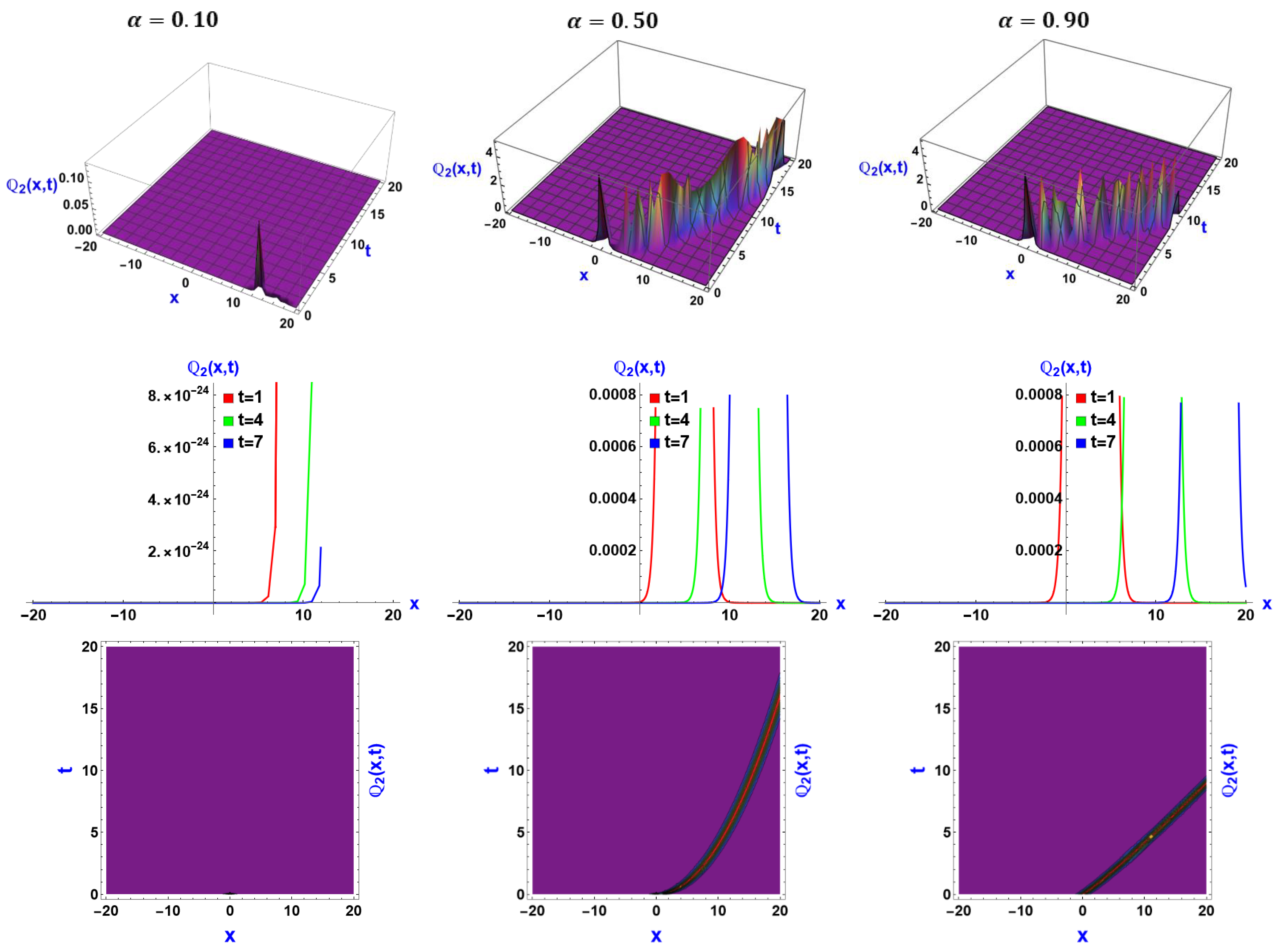
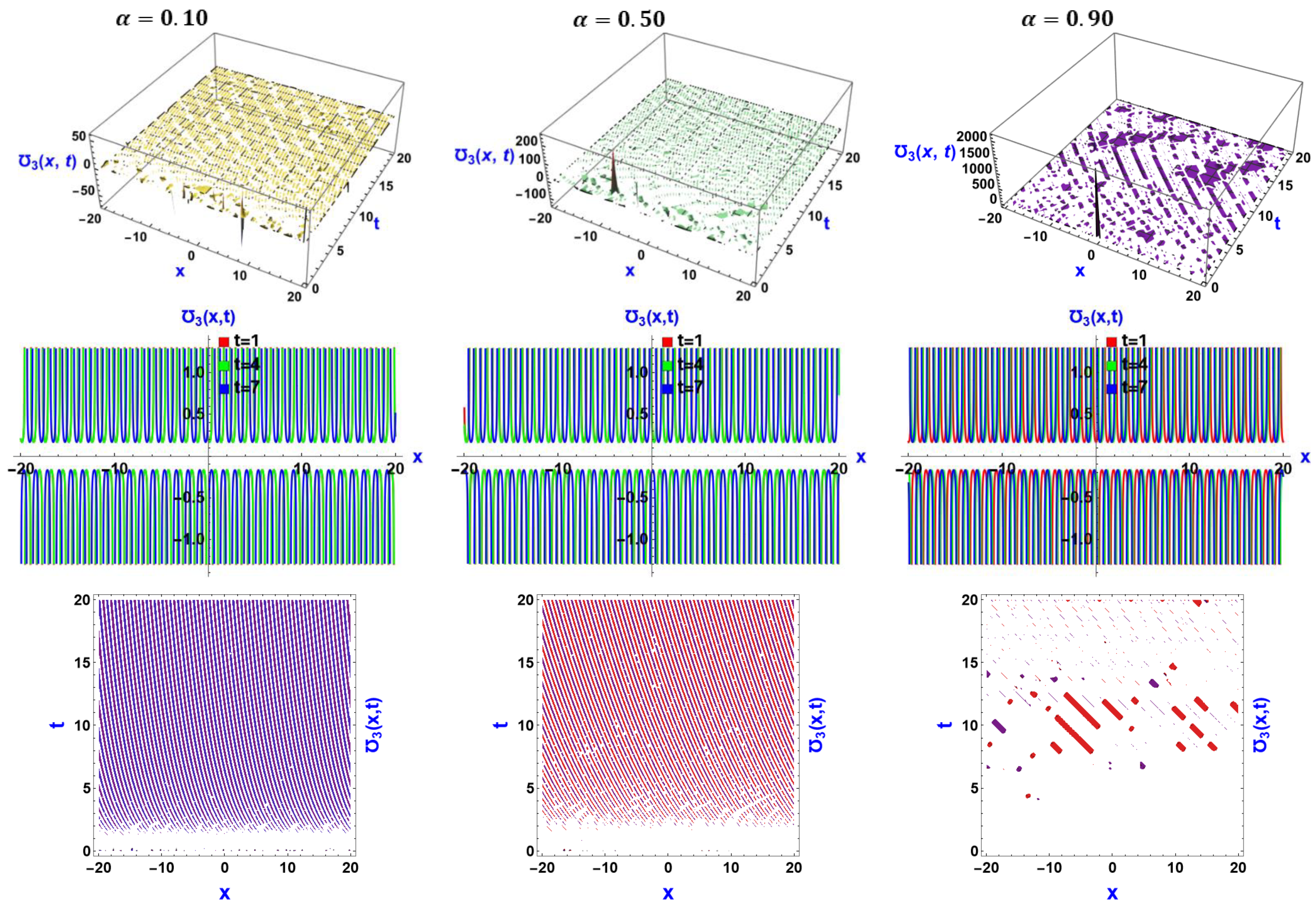
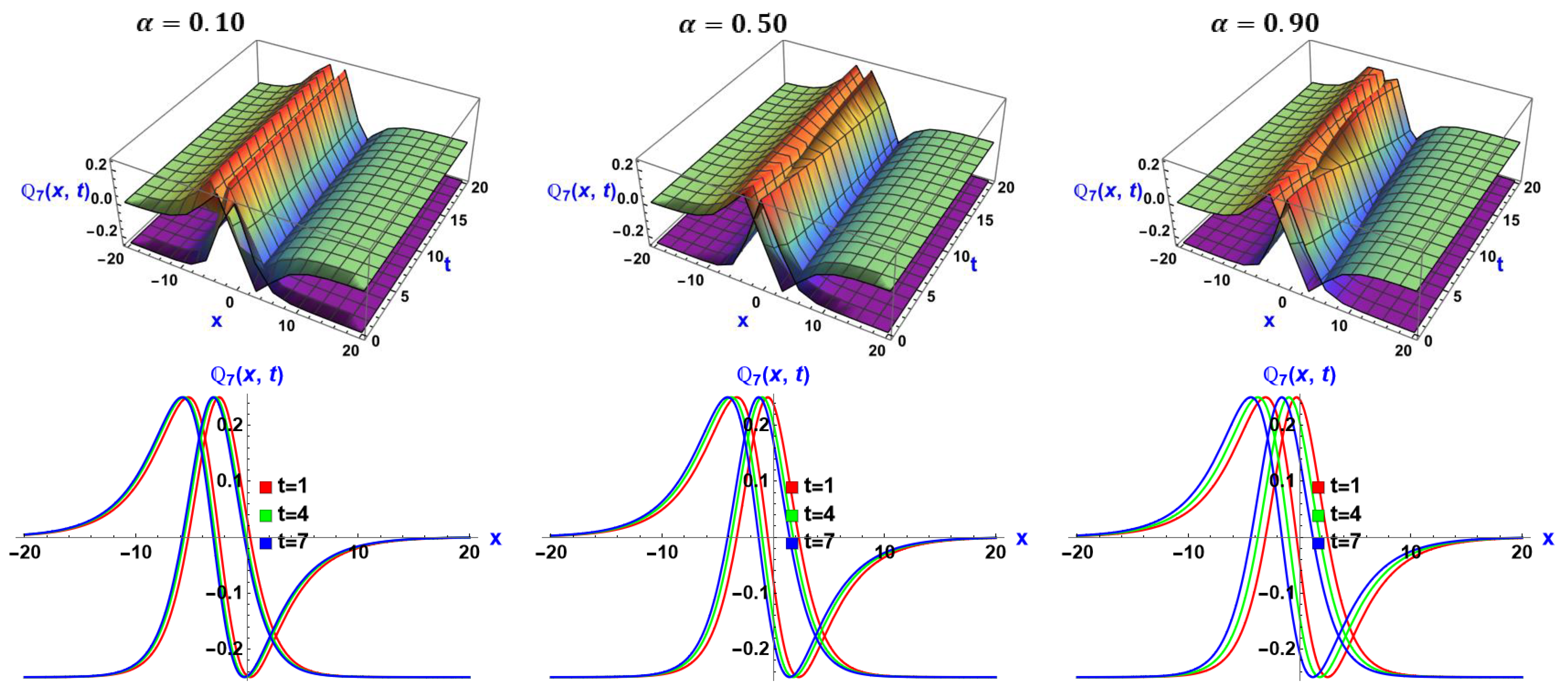
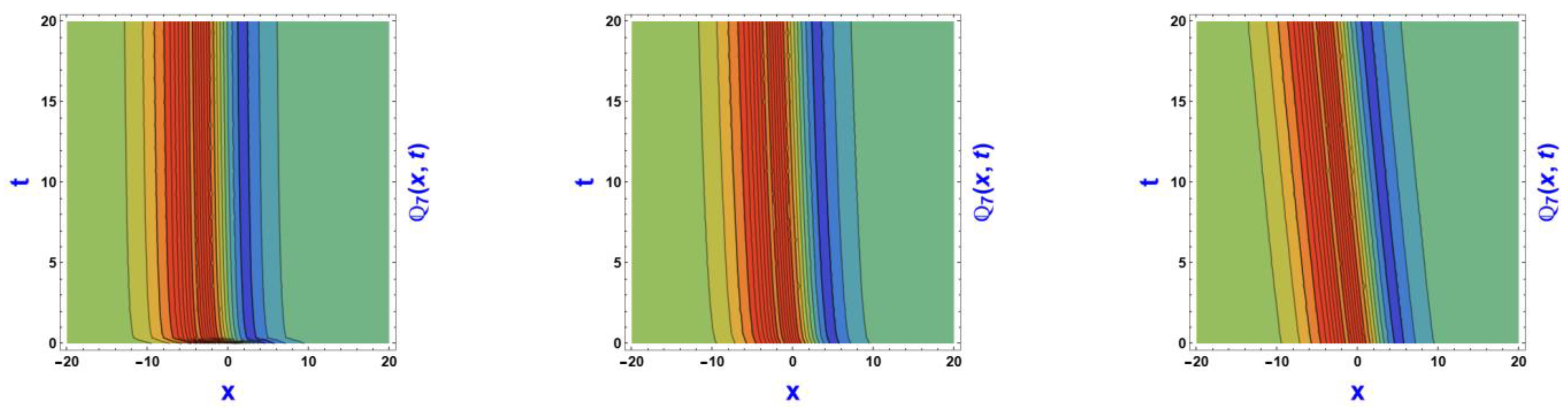
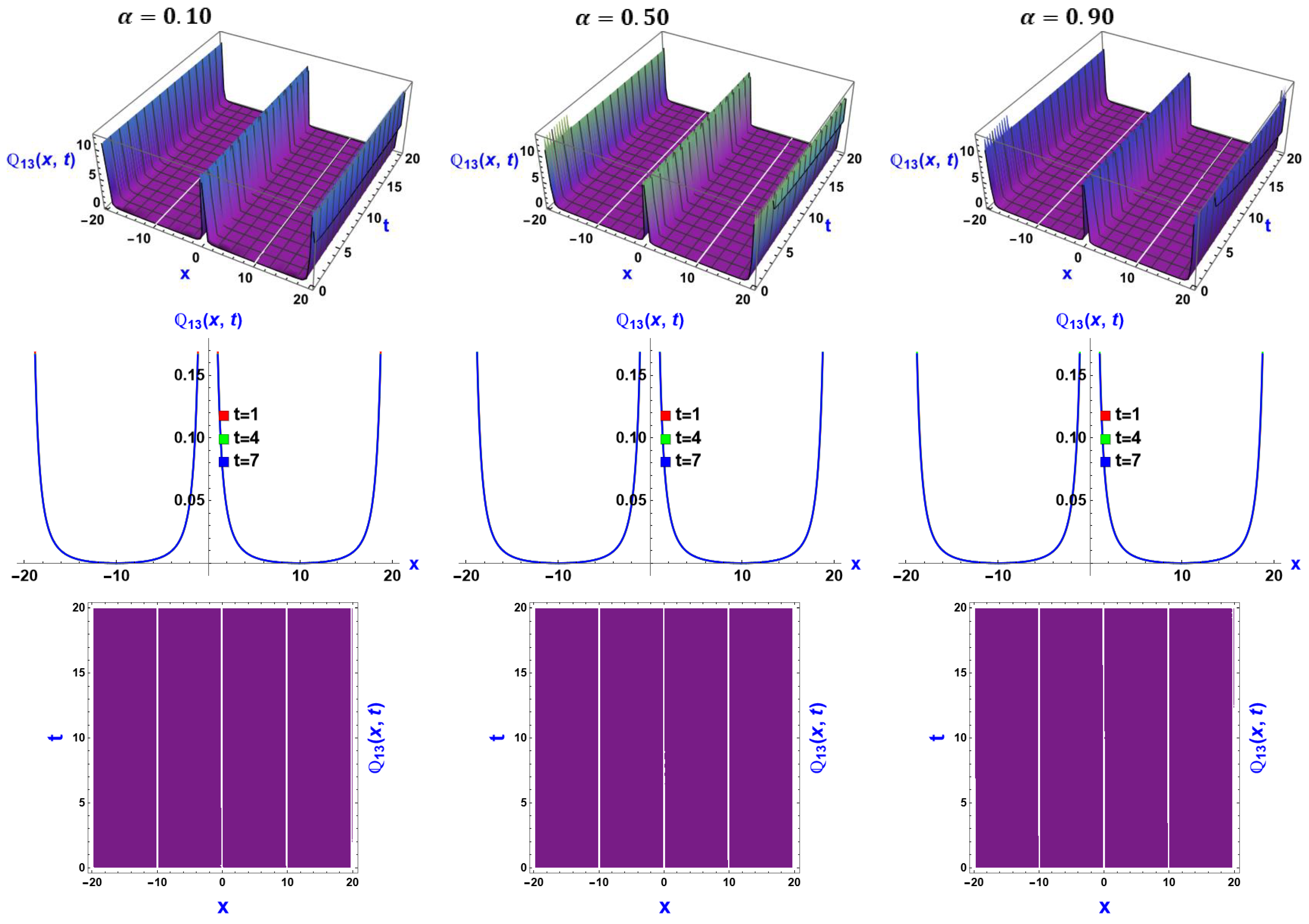
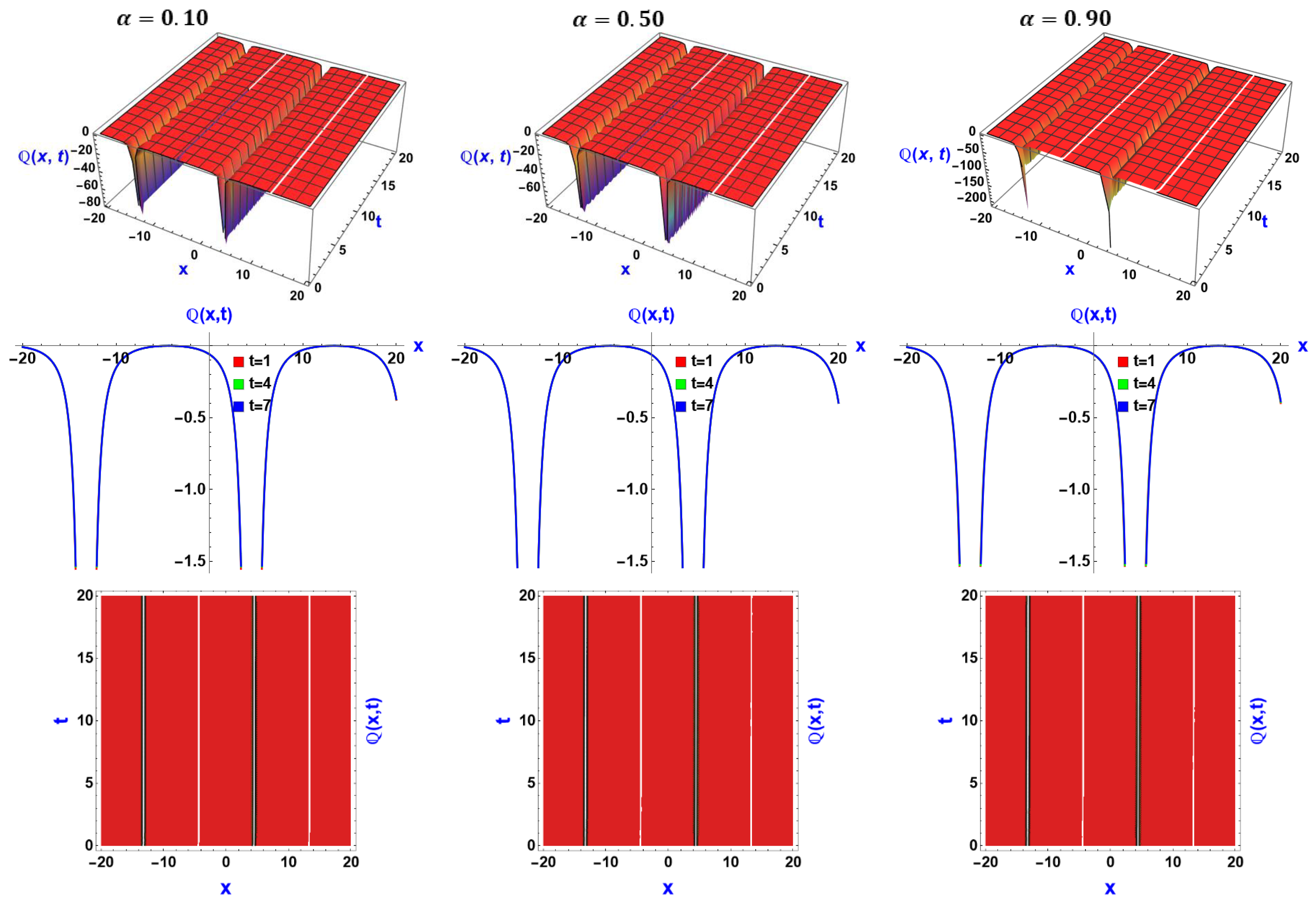
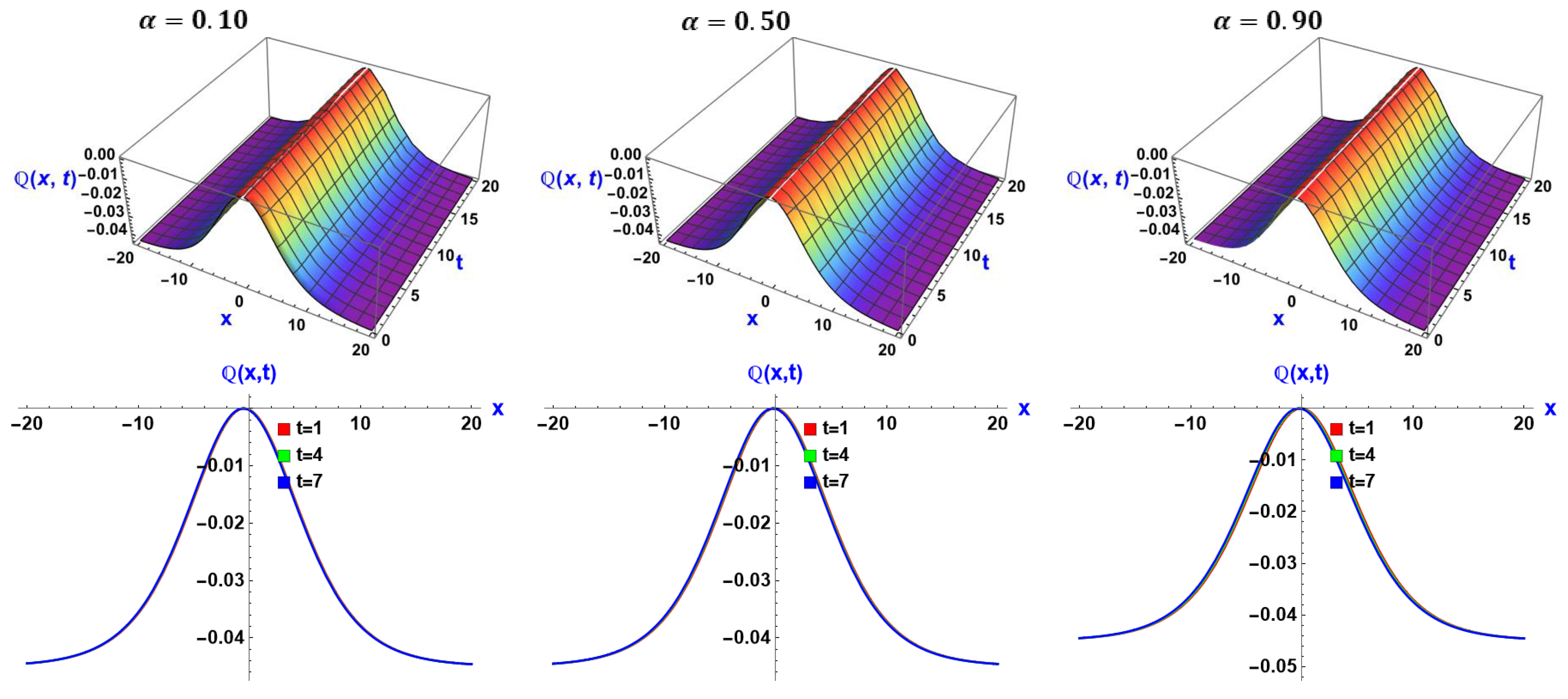
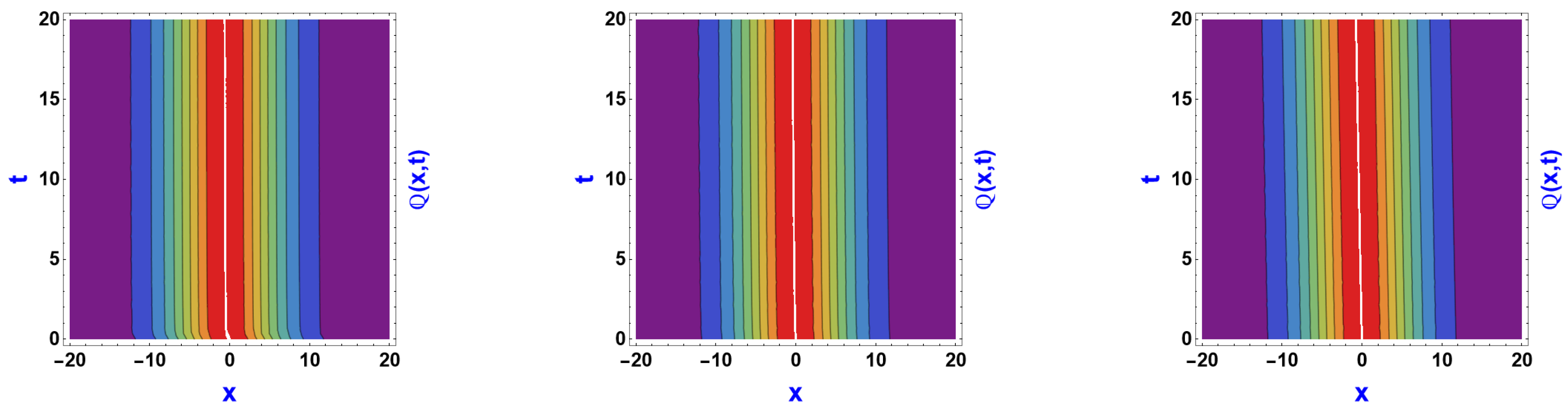
6. Visual Representation of the Exact Solutions

To visualize the exact solutions to the DSW equations using both methods, we utilized Mathematica, a sophisticated computational tool. This presentation includes a diverse range of visualizations, such as 3D renderings, 2D plots, and contour plots. To ensure clarity and conciseness, we selected four representative solution sets from the Sardar subequation method for each scenario and two from the $\left(\frac{{\mathsf{\Omega }}^{\prime }}{\mathsf{\Omega }}, \frac{1}{\mathsf{\Omega }}\right)$-expansion method for two scenarios. These graphs are depicted over the interval −20 ≤ (x, t) ≤ 20 for each case, with the corresponding constants provided in the figure captions. In the 2D plots, multiple solutions are combined within a single figure by varying the parameter t. Additionally, contour plots for each case are provided. For a better understanding, the fractional parameter $\alpha$ is set to 0.10, 0.50, and 0.90 for each case.

Discussions of the Graphs

In this study, the figures depict various soliton structures obtained using two distinct methodologies: the Sardar subequation technique and the $\left(\frac{{\mathit{\mho }}^{\mathit{\prime }}}{\mathit{\mho }},\frac{1}{\mathit{\mho }}\right)$ method. Concentrating on Figure 1, Figure 2, Figure 3 and Figure 4, which utilize the Sardar subequation technique, we observe a range of soliton behaviors with variations in the fractional parameter. Figure 1 illustrates the multi-singular type of soliton solution, while Figure 2 showcases the singular soliton. Additionally, Figure 3 demonstrates the combination of kink and bright solitons, and Figure 4 reveals a multiple bright-type soliton structure. These visualizations are primarily influenced by parameters such as $\varpi , s$, and $\sigma$, where higher positive values yield singular-type solitons, while higher negative values lead to dark-type solitons. The fractional parameter $\alpha$ plays a crucial role in altering the size and shape of the solitons, especially when it is close to 1, and vice versa.

Turning our attention to Figure 5 and Figure 6, which are derived using the $\left(\frac{{\mho }^{\prime }}{\mho }, \frac{1}{\mho }\right)$ method, we meet a different set of soliton structures. Figure 5 illustrates the multiple dark-type soliton solution, while Figure 6 shows bell-type soliton characteristics. In this method, the dominant parameters influencing soliton behavior are $\lambda$, $s$, and $\sigma$. Similarly, like the Sardar subequation method, the fractional parameter $\alpha$ significantly influences the size and shape of the solitons, with its effects being particularly pronounced when $\alpha$ is near 1. Conversely, these effects diminish as $\alpha$ moves away from 1.

The soliton solutions that we derived from Equation (1) exhibit a variety of forms, including kink, bright, dark, multiple dark, singular, multiple singular, and bell-shaped patterns. These solutions are essential in numerous fields, providing profound insights into system dynamics and fundamental physics. For instance, in condensed matter physics, kink solitons influence the behavior of magnetic domains, while, in nonlinear optics, dark and multiple dark solitons are used for high-speed data transmission. Furthermore, multiple singular, singular, and bell-shaped solitons are valuable in fluid dynamics and plasma physics, and bright solitons are crucial for predicting extreme wave events. Collectively, these soliton solutions contribute significantly to science, technology, and engineering, enhancing our comprehension of natural phenomena and driving technological progress.

7. Comparison

In this section, we examine the novelty and scientific contributions of our paper by comparing our findings with those in [6]. This comparison is organized into two parts, focusing on the similarities and differences between our studies. By identifying both the commonalities and distinctions, we aim to provide a thorough understanding of the unique insights our research brings to the field.

7.1. Uniformities

i.

Both studies center on the conformal time-fractional DSW equations, a crucial nonlinear complex model employed to analyze wave dynamics, particularly phenomena such as soliton propagation and interactions;

ii.

Both studies seek to derive exact solutions through analytical methods.

7.2. Variation and Uniqueness

i.

Reference [6] employed the modified extended tanh method (one variable) to derive exact solutions, whereas this study utilizes two efficient methods: the Sardar subequation method (one variable) and the $\left(\frac{{\mathsf{\Omega }}^{\prime }}{\mathsf{\Omega }},\frac{1}{\mathsf{\Omega }}\right)$-expansion technique (two variables);

ii.

While they only obtained multiple singular and bell-shaped solitons, this study includes a wider variety, such as kink, dark, multi-dark, bell-shaped, bright, multiple singular, and singular solitons;

iii.

This study presents a more diverse range of graphical representations, including 2D, 3D, and contour plots of exact solutions, whereas [6] utilized only 3D and density diagrams.

8. Conclusions

In this investigation, we uncovered a series of innovative exact solutions to the DSW equation by employing two versatile methods: the Sardar subequation method (utilizing one variable) and the $\left(\frac{{\mathsf{\Omega }}^{\prime }}{\mathsf{\Omega }},\frac{1}{\mathsf{\Omega }}\right)$-expansion method (employing two variables). These methodologies enabled the construction of a diverse array of solutions, incorporating trigonometric, rational, and hyperbolic functions. Rigorous validation procedures conducted with Mathematica software ensured precision, while dynamic visual representations vividly depicted the soliton solutions, showcasing a rich variety of patterns such as dark, multiple dark, singular, multiple singular, kink, and bell-shaped solitons. These derived solutions offer a distinctive perspective, surpassing conventional approaches and presenting a more nuanced portrayal of the dynamic behavior inherent in the DSW equations. Leveraging computational techniques significantly bolstered our understanding of the equation’s dynamics, underscoring their substantial contribution to our comprehension. The established solutions, confirmed through contour, 2D, and 3D plots, underscored the effectiveness of these methods in identifying novel soliton solutions, accurately characterizing their properties and providing deeper insights into the model’s behavior. The soliton solutions obtained in this study hold promise for advancing technology and engineering, easing a deeper understanding of natural phenomena and driving innovation within the realm of the DSW equations. These findings not only hold the potential for enhancing technological capabilities, but also contribute to a more profound understanding of complex nonlinear dynamics. Looking ahead, these soliton solutions offer exciting opportunities for fostering innovation and further exploration across various scientific and engineering disciplines.

References

1. Khater, M.M.A. Soliton Propagation under Diffusive and Nonlinear Effects in Physical Systems; (1+1)–Dimensional MNW Integrable Equation. Phys. Lett. Sect. A Gen. At. Solid State Phys. 2023, 480, 128945. [Google Scholar] [CrossRef]
2. Chahlaoui, Y.; Ali, A.; Ahmad, J.; Hussain, R.; Javed, S. Dynamical Behavior of Optical Soliton Solutions, Time Series and Sensitivity Analysis to the Schrödinger Model with Eta Fractional Derivative. Opt. Quantum Electron. 2024, 56, 704. [Google Scholar] [CrossRef]
3. Islam, S.M.R.; Wang, H. Some Analytical Soliton Solutions of the Nonlinear Evolution Equations. J. Ocean Eng. Sci. 2022, 1–9. [Google Scholar] [CrossRef]
4. Hossain, M.N.; Alsharif, F.; Miah, M.M.; Kanan, M. Abundant New Optical Soliton Solutions to the Biswas—Milovic Equation with Sensitivity Analysis for Optimization. Mathematics 2024, 12, 1585. [Google Scholar] [CrossRef]
5. Noor, S.; Alshehry, A.S.; Dutt, H.M.; Nazir, R.; Khan, A.; Shah, R. Investigating the Dynamics of Time-Fractional Drinfeld–Sokolov–Wilson System through Analytical Solutions. Symmetry 2023, 15, 703. [Google Scholar] [CrossRef]
6. Bashar, M.H.; Mawa, H.Z.; Biswas, A.; Rahman, M.M.; Roshid, M.M.; Islam, J. The Modified Extended Tanh Technique Ruled to Exploration of Soliton Solutions and Fractional Effects to the Time Fractional Couple Drinfel’d–Sokolov–Wilson Equation. Heliyon 2023, 9, e15662. [Google Scholar] [CrossRef]
7. Ali, A.; Ahmad, J.; Javed, S. Exploring the Dynamic Nature of Soliton Solutions to the Fractional Coupled Nonlinear Schrödinger Model with Their Sensitivity Analysis. Opt. Quantum Electron. 2023, 55, 810. [Google Scholar] [CrossRef]
8. Baleanu, D.; Agarwal, R.P. Fractional Calculus in the Sky. Adv. Differ. Equ. 2021, 2021, 117. [Google Scholar] [CrossRef]
9. Shahzad, M.U.; Rehman, H.U.; Awan, A.U.; Zafar, Z.; Hassan, A.M.; Iqbal, I. Analysis of the Exact Solutions of Nonlinear Coupled Drinfeld–Sokolov–Wilson Equation through Φ^6-Model Expansion Method. Results Phys. 2023, 52, 106771. [Google Scholar] [CrossRef]
10. Chen, S.; Liu, Y.; Wei, L.; Guan, B. Exact Solutions to Fractional Drinfel’d–Sokolov–Wilson Equations. Chin. J. Phys. 2018, 56, 708–720. [Google Scholar] [CrossRef]
11. Shakeel, M.; AlQahtani, S.A.; Rehman, M.J.U.; Kudra, G.; Awrejcewicz, J.; Alawwad, A.M.; A.Alotaibi, A.; Safran, M. Construction of Diverse Water Wave Structures for Coupled Nonlinear Fractional Drinfel’d-Sokolov-Wilson Model with Beta Derivative and Its Modulus Instability. Sci. Rep. 2023, 13, 17528. [Google Scholar] [CrossRef] [PubMed]
12. Kawser, M.A.; Ali Akbar, M.; Khan, M.A.; Ghazwan, H.A. Exact Soliton Solutions and the Signifcance of Time-dependent Coefcients in the Boussinesq Equation: Theory and Application in Mathematical Physics. Sci. Rep. 2024, 14, 762. [Google Scholar] [CrossRef] [PubMed]
13. Borhan, J.R.M.; Ganie, A.H.; Miah, M.M.; Iqbal, M.A.; Seadawy, A.R.; Mishra, N.K. A Highly Effective Analytical Approach to Innovate the Novel Closed Form Soliton Solutions of the Kadomtsev–Petviashivili Equations with Applications. Opt. Quantum Electron. 2024, 56, 938. [Google Scholar] [CrossRef]
14. Iqbal, M.A.; Miah, M.M.; Rasid, M.M.; Alshehri, H.M.; Osman, M.S. An Investigation of Two Integro-Differential KP Hierarchy Equations to Find out Closed Form Solitons in Mathematical Physics. Arab J. Basic Appl. Sci. 2023, 30, 535–545. [Google Scholar] [CrossRef]
15. Ma, W.X. N-Soliton Solutions and the Hirota Conditions in (1 + 1)-Dimensions. Int. J. Nonlinear Sci. Numer. Simul. 2022, 23, 123–133. [Google Scholar] [CrossRef]
16. Yomba, E. The General Projective Riccati Equations Method and Exact Solutions for a Class of Nonlinear Partial Differential Equations. Chin. J. Phys. 2005, 43, 991–1003. [Google Scholar]
17. Jafari, H.; Kadkhoda, N.; Baleanu, D. Fractional Lie Group Method of the Time-Fractional Boussinesq Equation. Nonlinear Dyn. 2015, 81, 1569–1574. [Google Scholar] [CrossRef]
18. Zafar, A.; Raheel, M.; Ali, K.K.; Razzaq, W. On Optical Soliton Solutions of New Hamiltonian Amplitude Equation via Jacobi Elliptic Functions. Eur. Phys. J. Plus 2020, 135, 674. [Google Scholar] [CrossRef]
19. Khan, M.A.U.; Akram, G.; Sadaf, M. Dynamics of Novel Exact Soliton Solutions of Concatenation Model Using Efective Techniques. Opt. Quantum Electron. 2024, 56, 385. [Google Scholar] [CrossRef]
20. Babajanov, B.; Abdikarimov, F. The Application of the Functional Variable Method for Solving the Loaded Non-Linear Evaluation Equations. Front. Appl. Math. Stat. 2022, 8, 912674. [Google Scholar] [CrossRef]
21. Ma, W.X.; Zhu, Z. Solving the (3 + 1)-Dimensional Generalized KP and BKP Equations by the Multiple Exp-Function Algorithm. Appl. Math. Comput. 2012, 218, 11871–11879. [Google Scholar] [CrossRef]
22. Islam, S.M.R.; Arafat, S.M.Y.; Wang, H. Abundant Closed-Form Wave Solutions to the Simplified Modified Camassa-Holm Equation. J. Ocean Eng. Sci. 2023, 8, 238–245. [Google Scholar] [CrossRef]
23. Fan, E. Extended Tanh-Function Method and Its Applications to Nonlinear Equations. Phys. Lett. A 2000, 277, 212–218. [Google Scholar] [CrossRef]
24. Nofal, T.A. Simple Equation Method for Nonlinear Partial Differential Equations and Its Applications. J. Egypt. Math. Soc. 2016, 24, 204–209. [Google Scholar] [CrossRef]
25. Kumar, A.; Pankaj, R.D. Tanh–Coth Scheme for Traveling Wave Solutions for Nonlinear Wave Interaction Model. J. Egypt. Math. Soc. 2015, 23, 282–285. [Google Scholar] [CrossRef]
26. Habib, M.A.; Ali, H.M.S.; Miah, M.M.; Akbar, M.A. The Generalized Kudryashov Method for New Closed Form Traveling Wave Solutions to Some NLEEs. AIMS Math. 2019, 4, 896–909. [Google Scholar] [CrossRef]
27. Fokas, A.S.; Lenells, J. The Unified Method: I. Nonlinearizable Problems on the Half-Line. J. Phys. A Math. Theor. 2012, 45, 195201. [Google Scholar] [CrossRef]
28. Santillana, M.; Dawson, C. A Numerical Approach to Study the Properties of Solutions of the Diffusive Wave Approximation of the Shallow Water Equations. Comput. Geosci. 2010, 14, 31–53. [Google Scholar] [CrossRef]
29. Ren, B.; Lou, Z.M.; Liang, Z.F.; Tang, X.Y. Nonlocal Symmetry and Explicit Solutions for Drinfel’d-Sokolov-Wilson System. Eur. Phys. J. Plus 2016, 131, 441. [Google Scholar] [CrossRef]
30. Zhao, X.Q.; Zhi, H.Y. An Improved F-Expansion Method and Its Application to Coupled Drinfel’d-Sokolov-Wilson Equation. Commun. Theor. Phys. 2008, 50, 309–314. [Google Scholar] [CrossRef]
31. Sahoo, S.; Ray, S.S. New Double-Periodic Solutions of Fractional Drinfeld–Sokolov–Wilson Equation in Shallow Water Waves. Nonlinear Dyn. 2017, 88, 1869–1882. [Google Scholar] [CrossRef]
32. Inc, M. On Numerical Doubly Periodic Wave Solutions of the Coupled Drinfel’d-Sokolov-Wilson Equation by the Decomposition Method. Appl. Math. Comput. 2006, 172, 421–430. [Google Scholar] [CrossRef]
33. Rehman, H.U.; Habib, A.; Ali, K.; Awan, A.U. Study of Langmuir Waves for Zakharov Equation Using Sardar Sub-Equation Method. Int. J. Nonlinear Anal. Appl. 2023, 14, 9–18. [Google Scholar]
34. Yasin, S.; Khan, A.; Ahmad, S.; Osman, M.S. New Exact Solutions of (3+1)-Dimensional Modified KdV-Zakharov-Kuznetsov Equation by Sardar-Subequation Method. Opt. Quantum Electron. 2024, 56, 90. [Google Scholar] [CrossRef]
35. Rezazadeh, H.; Inc, M.; Baleanu, D. New Solitary Wave Solutions for Variants of (3+1)-Dimensional Wazwaz-Benjamin-Bona-Mahony Equations. Front. Phys. 2020, 8, 332. [Google Scholar] [CrossRef]
36. Rehman, H.U.; Iqbal, I.; Subhi Aiadi, S.; Mlaiki, N.; Saleem, M.S. Soliton Solutions of Klein–Fock–Gordon Equation Using Sardar Subequation Method. Mathematics 2022, 10, 3377. [Google Scholar] [CrossRef]
37. Ibrahim, S.; Ashir, A.M.; Sabawi, Y.A.; Baleanu, D. Realization of Optical Solitons from Nonlinear Schrödinger Equation Using Modified Sardar Sub-Equation Technique. Opt. Quantum Electron. 2023, 55, 617. [Google Scholar] [CrossRef]
38. Cinar, M.; Secer, A.; Ozisik, M.; Bayram, M. Derivation of Optical Solitons of Dimensionless Fokas-Lenells Equation with Perturbation Term Using Sardar Sub-Equation Method. Opt. Quantum Electron. 2022, 54, 402. [Google Scholar] [CrossRef]
39. Sadaf, M.; Arshed, S.; Ghazala Akram, I. Exact Soliton and Solitary Wave Solutions to the Fokas System Using Two Variables (G′/G,1/G)-Expansion Technique and Generalized Projective Riccati Equation Method. Opt.-Int. J. Light Electron Opt. 2022, 268, 169713. [Google Scholar] [CrossRef]
40. Vivas-Cortez, M.; Akram, G.; Sadaf, M.; Arshed, S.; Rehan, K.; Farooq, K. Traveling Wave Behavior of New (2+1)-Dimensional Combined KdV–MKdV Equation. Results Phys. 2023, 45, 106244. [Google Scholar] [CrossRef]
41. Miah, M.M.; Ali, H.M.S.; Akbar, M.A.; Wazwaz, A.M. Some Applications of the (G’/G, 1/G)-Expansion Method to Find New Exact Solutions of NLEEs. Eur. Phys. J. Plus 2017, 132, 252. [Google Scholar] [CrossRef]
42. Sirisubtawee, S.; Koonprasert, S.; Sungnul, S. Some Applications of the (G’/G, 1/G)-Expansion Method for Finding Exact Traveling Wave Solutions of Nonlinear Fractional Evolution Equations. Symmetry 2019, 11, 952. [Google Scholar] [CrossRef]
43. Rasid, M.M.; Miah, M.M.; Ganie, A.H.; Alshehri, H.M.; Osman, M.S.; Ma, W.X. Further Advanced Investigation of the Complex Hirota-Dynamical Model to Extract Soliton Solutions. Mod. Phys. Lett. B 2023, 38, 2450074. [Google Scholar] [CrossRef]
44. Hossain, M.N.; Miah, M.M.; Duraihem, F.Z.; Rehman, S. Stability, Modulation Instability, and Analytical Study of the Confirmable Time Fractional Westervelt Equation and the Wazwaz Kaur Boussinesq Equation. Opt. Quantum Electron. 2024, 56, 948. [Google Scholar] [CrossRef]
45. Hossain, M.N.; Miah, M.M.; Hamid, A.; Osman, G.M.S. Discovering New Abundant Optical Solutions for the Resonant Nonlinear Schrödinger Equation Using an Analytical Technique. Opt. Quantum Electron. 2024, 56, 847. [Google Scholar] [CrossRef]
46. Khalil, R.; Al Horani, M.; Yousef, A.; Sababheh, M. A New Definition of Fractional Derivative. J. Comput. Appl. Math. 2014, 264, 65–70. [Google Scholar] [CrossRef]
47. Abdeljawad, T. On Conformable Fractional Calculus. J. Comput. Appl. Math. 2015, 279, 57–66. [Google Scholar] [CrossRef]
Figure 1. Graphical behavior of multiple singular solitons of Q 2 x , t in 3D, 2D, and contour plots, where β = σ = ϱ = δ = g = l = 1 ,   ϖ = 5.1 , and s = 0.7 .
Fractalfract 08 00352 g001
Figure 2. Variation of singular soliton with the fractional parameter of 3 x , t in 3D, 2D, and contour plots, where β = ϱ = δ = 3 ,   σ = 0.1 ,   g = l = 0.1 ,   ϖ = 0.5 , and s = 7.1 .
Fractalfract 08 00352 g002
Figure 3. The change in kink and bright soliton behavior with the fractional parameter of Q 2 x , t in 3D, 2D, and contour plots, where β = ϱ = δ = 1 ,   σ = 5.0 ,   g = l = 1 ,   ϖ = 0.3 , and s = 0.5 .
Fractalfract 08 00352 g003aFractalfract 08 00352 g003b
Figure 4. The variation in behavior of multiple periodic bright-type solitons with the fractional parameter of Q 13 x , t in 3D, 2D, and contour plots, where β = ϱ = δ = 1 ,   σ = 0.1 ,   g = l = 1 ,   ϖ = 5 , and s = 0.1 .
Fractalfract 08 00352 g004
Figure 5. The evolution of multiple periodic dark-type solitons in response to changes in the fractional parameter in Equation (67) in 3D, 2D, and contour plots, where β = 1 ,   ϱ = δ = σ = 0.1 ,   λ = 0.01 , and s = 3.55 .
Fractalfract 08 00352 g005
Figure 6. The variation of bell-type solitons in response to changes in the fractional parameter in Equation (74) in 3D, 2D, and contour plots, where β = ϱ = δ = σ = 1 ,   λ = 1 , and s = 0.3 .
Fractalfract 08 00352 g006aFractalfract 08 00352 g006b
Disclaimer/Publisher’s Note: The statements, opinions and data contained in all publications are solely those of the individual author(s) and contributor(s) and not of MDPI and/or the editor(s). MDPI and/or the editor(s) disclaim responsibility for any injury to people or property resulting from any ideas, methods, instructions or products referred to in the content.