Abstract
The accurate recognition of a brain tumor (BT) is crucial for accurate diagnosis, intervention planning, and the evaluation of post-intervention outcomes. Conventional methods of manually identifying and delineating BTs are inefficient, prone to error, and time-consuming. Subjective methods for BT recognition are biased because of the diffuse and irregular nature of BTs, along with varying enhancement patterns and the coexistence of different tumor components. Hence, the development of an automated diagnostic system for BTs is vital for mitigating subjective bias and achieving speedy and effective BT segmentation. Recently developed deep learning (DL)-based methods have replaced subjective methods; however, these DL-based methods still have a low performance, showing room for improvement, and are limited to heterogeneous dataset analysis. Herein, we propose a DL-based parallel features aggregation network (PFA-Net) for the robust segmentation of three different regions in a BT scan, and we perform a heterogeneous dataset analysis to validate its generality. The parallel features aggregation (PFA) module exploits the local radiomic contextual spatial features of BTs at low, intermediate, and high levels for different types of tumors and aggregates them in a parallel fashion. To enhance the diagnostic capabilities of the proposed segmentation framework, we introduced the fractal dimension estimation into our system, seamlessly combined as an end-to-end task to gain insights into the complexity and irregularity of structures, thereby characterizing the intricate morphology of BTs. The proposed PFA-Net achieves the Dice scores (DSs) of 87.54%, 93.42%, and 91.02%, for the enhancing tumor region, whole tumor region, and tumor core region, respectively, with the multimodal brain tumor segmentation (BraTS)-2020 open database, surpassing the performance of existing state-of-the-art methods. Additionally, PFA-Net is validated with another open database of brain tumor progression and achieves a DS of 64.58% for heterogeneous dataset analysis, surpassing the performance of existing state-of-the-art methods.
1. Introduction
An uncontrolled growth of cancerous or non-cancerous cells inside a rigid skull characterizes a brain tumor (BT). Computer-aided diagnostic (CAD) tools, when coupled with artificial intelligence (AI) techniques, play a crucial role in facilitating its early detection [1]. The World Health Organization (WHO) has classified BTs into four grades, one–four, and further categorized them into high-grade glioma (HGG) and low-grade glioma (LGG) based on the malignancy scale of pathological tissues [2]. HGGs are aggressive BTs with high mortality rates [3]. Data from the National Program of Cancer Registries (NPCR) and the Surveillance, Epidemiology, and End Results (SEER) registries revealed that between 2008 and 2017, 54% of adults in the United States were identified with HGGs, whereas the occurrence rate of HGGs in young individuals ranged from 0.5% to 0.7% [4]. On the other hand, LGGs are slow growing and less fatal, and patients with LGGs have a long survival period compared to those with HGGs; however, if LGGs are not recognized and treated at their earlier stages, they infiltrate into neighboring cells, relapse, and finally advance to HGGs [5]. Invasive treatments for BTs, such as surgery, increase the likelihood of gross total resection (GTR) but carry the risk of damaging crucial brain regions responsible for speech and mobility, while non-invasive treatments for BTs, such as radiotherapy, if not precisely targeted, can severely affect vision, hormone levels, and brain function [6,7]. The research in the selection of these treatments, the accurate recognition of BTs, mental condition estimation, and motor imagery using AI can improve survival outcomes [8].
Conventional methods of manually identifying and delineating BTs are inefficient and subjective because of the complex anatomy of the tumor, its infiltration into normal tissue, and the diverse information obtained from different magnetic resonance imaging (MRI) scans. The diffusion and irregular nature of BTs, along with varying enhancement patterns and the coexistence of different tumor components, pose additional challenges in accurate recognition and treatment. Therefore, the accurate identification of BT location and morphology is crucial for accurate assessment, intervention planning, and the evaluation of post-intervention outcomes. Thus, the development of a CAD tool for BT is desirable for mitigating subjective bias and achieving speedy and effective BT segmentation [9]. Developing a CAD tool for MRI scans of LGG and HGG is challenging because of several factors. These include the complex anatomy of the BT, which varies from one patient to another, the infiltration of normal tissue, and diverse intensities of information from different MRI modalities that require expert interpretation [10].
Segmentation analysis involves breaking down an image into different parts to understand them better. BT segmentation analysis helps doctors identify and locate the tumor accurately. Deep learning (DL) models are like smart tools that learn from examples to automatically recognize patterns in images. In BT analysis, these models are trained to spot and outline tumors in MRI scans. In this paper, we are using algorithms based on DL to help doctors pinpoint and understand these tumors in MRI scans. Convolutional neural networks (CNNs) have demonstrated the ability to learn and recognize intricate patterns in medical images, thereby achieving superior performance in classification and segmentation [11,12,13,14]. A CNN is a DL algorithm that uses convolutional layers to perform localized feature extraction, pooling layers to reduce spatial dimensions while preserving essential information, and fully connected layers to make high-level predictions [15].
Several CAD frameworks have been developed for BT classification and segmentation based on hand- and DL-extracted features methods [16,17,18,19,20,21]. We propose a CAD tool utilizing DL-extracted features for the robust segmentation of three different BT regions of the multimodal brain tumor segmentation (BraTS)-2020 dataset [9,22,23]. The three regions, named enhancing tumor (ET), whole tumor (WT), and tumor core (TC), are challenging to segment from a scan owing to diffused, irregular, and non-specific enhancement, varying distribution, heterogeneity, and the coexistence of different tumor components. Furthermore, class imbalance presents a significant challenge, owing to the small size of the tumor areas and their vulnerability to background domination.
Existing methods have not shown satisfactory performance, particularly in the case of ET. Additionally, existing methods do not perform a heterogeneous dataset analysis, which is crucial for determining the generalizability of a CAD framework. We designed a DL-based parallel features aggregation network (PFA-Net) to decrease the likelihood of GTR, minimize subjective bias, and perform robust BT segmentation. Moreover, we performed a heterogeneous dataset analysis to validate the generality of the proposed CAD framework. Mainly, we have introduced a novel module based on parallel feature aggregation, which employs multiple-branch feature extraction operations to extract discriminative information from BT scans simultaneously with the aggregation of them. Specifically, we utilize three of these modules at different levels within the encoder of the proposed segmentation framework to capture spatial semantic information at various levels. Additionally, one module is incorporated into the decoder of the segmentation framework to handle the diverse information obtained from the encoder. The detailed working and architecture of the proposed module are described in Section 3.
The fractal dimension (FD) is widely used across various fields, including biology [24], medical image analysis [25], urbanization studies [26], and the identification of BTs [27]. In our study, we introduced the FD estimation in our segmentation framework. This analysis provides valuable insights into the structural complexity and irregularity of BTs. By characterizing the intricate morphology of BTs, it enhances understanding of BT behavior and aids in diagnostic and prognostic assessments, ultimately contributing to advancements in BT research and patient care.
The experimental outcomes demonstrate that the proposed method significantly enhances the overall segmentation accuracy, both qualitatively and quantitatively. This study addresses the limitations of previous studies and outperform them with the following novelties:
- -
- This study proposes a robust CAD framework based on radiomic parallel features aggregation for the accurate segmentation of three different BT regions. The framework comprises an encoder–decoder architecture, with a novel PFA block comprising multiple-branch feature extraction layers to learn discriminative information from the BT scans in parallel and aggregate them.
- -
- In the encoder module, the PFA block is integrated at low, intermediate, and high levels to capture a comprehensive representation of the BT and preserve diverse multi-level information throughout the encoding process. The multi-level aggregated features capture the overall characteristics of the BT, incorporating local details, such as small tumor boundaries, particularly for ET, intermediate-level structures, such as the shape of the BT, and high-level global information, such as the overall location and size of the BT.
- -
- In contrast to the encoder module, the decoder module utilizes the PFA block to collectively process upscaled low-level, intermediate-level, and high-level bottleneck-rich semantic features in parallel. Subsequently, the PFA block aggregates these semantic features to ensure that the decoder module has access to a diverse range of information, including fine-grained details and high-level contexts.
- -
- Our proposed PFA-Net surpasses the state-of-the-art methods in the field of heterogeneous dataset analysis in terms of segmentation performance and computational efficiency, with 19.49 million (M) parameters less than those of the previous method.
- -
- The integration of the FD estimation method into our system provides valuable insights into the distributional characteristics of BTs, thereby enhancing the comprehensiveness of our approach. Moreover, our trained PFA-Net is publicly available for fair comparison via the following link (https://github.com/PFA-Net, accessed on 23 November 2023).
The proposed framework offers novelty in several key aspects. Firstly, it presents a robust CAD system named PFA-Net, which employs radiomic parallel features aggregation to accurately segment three distinct regions within BTs. This innovative approach strategically integrates a PFA block within an encoder–decoder architecture, positioned at multiple levels to capture comprehensive BT representations, while retaining multi-level information throughout encoding. Notably, the framework outperforms state-of-the-art methods in both homogeneous and heterogeneous dataset analyses, demonstrating superior segmentation performance and computational efficiency. Furthermore, the incorporation of the FD estimation method provides valuable insights into the distributional characteristics of BTs, enhancing the overall comprehensiveness of the framework. In conclusion, this framework signifies a significant advancement in BT segmentation by amalgamating innovative techniques (PFA-Net and FD) to achieve heightened accuracy and efficiency.
The rest of this paper is organized as follows: Section 2 presents a review of related work on BT segmentation. Section 3 presents our method, and Section 4 presents the experimental results with an in-depth analysis. Section 5 discusses the main findings and limitations of this study. Finally, Section 6 wraps up the paper by presenting a summary of the main findings and describing the future scope of research.
2. Related Work
Several CNN-based methods have been developed for classification and segmentation in BT screening. In this study, we considered CNN-based methods for BT segmentation using homogeneous and heterogeneous datasets. Homogeneous dataset segmentation refers to the segmentation of three different BT regions of the BraTS-2020 dataset. By contrast, a heterogeneous dataset refers to the utilization of different datasets for training and testing in a heterogeneous analysis environment.
2.1. Homogeneous Dataset Analysis
Most of the research conducted on the segmentation task of the BraTS-2020 dataset has focused on using modified versions of the two-dimensional (2D) U-Net [28] and the three-dimensional (3D) U-Net [29]. U-Net architectures have proven to be highly effective for medical image segmentation tasks, including BT segmentation. While modified versions of U-Net have been the dominant choices, few studies have explored alternative CNN architectures for the same problem. These methods compare the performance of different CNN models and evaluate their suitability for BraTS-2020 dataset segmentation. This section decodes the dichotomy between handcrafted feature-based and deep feature-based methods for BT classification, localization, and segmentation.
2.1.1. Handcrafted Feature-Based Methods
Before the advent of DL techniques, BTs were identified and analyzed using conventional image processing techniques. For example, Velthuizen et al. [30] compared the performance of supervised machine learning (ML) methods, including K-nearest neighbor (kNN) and region growing, with unsupervised ML methods, including non-fuzzy clustering and the fuzzy C-means algorithm, for measuring tumor volumes in a dataset of MRI of 10 patients. They concluded the supervised methods were superior to unsupervised ones in terms of true positive rate. However, unsupervised methods required a large processing time. Kamber et al. [31] proposed model-based and non-model-based methods to automatically segment multiple sclerosis lesions in MRI of the human brain. They used different classifiers including a decision tree, Bayesian classifier, and statistical minimum distance. The MR image data were pre-processed by applying homomorphic filters to remove inhomogeneity artifacts, and segmentation errors were manually corrected. Gibbs et al. [32] used different image processing morphological routines, including a Sobel edge filter, region growing algorithm, and nearest-neighbor filters, for segmentation of glioma from 10 patients’ data in MRI volumes. Their segmentation results were not compared with the ground truth, and therefore lacked authenticity. Clark et al. [33] designed a knowledge-based segmentation system for glioblastoma-multiforme tumors using unsupervised clustering methods and multispectral histograms. This process involves knowledge engineering, wherein we determine the most useful knowledge for the goal of tumor segmentation and then implement this information into a rule-based system. Their system generated many false-positive (FP) cases.
Kaus et al. [34] developed a computerized segmentation technique for LGGs and meningiomas. Their method was a combination of a statistical classification approach along with digital atlas knowledge. The automated method demonstrates comparable accuracy to the manual method in segmenting the brain and tumor, along with improved reproducibility, but their method was dependent on an atlas. Warfield et al. [35] developed a novel adaptive, template-moderated statistical method for the segmentation of normal anatomy and abnormal anatomy from MRI scans of the brain, knee cartilage, and sclerosis. Their method was dependent on an external template, and pre-processing was needed. Mazzara et al. [36] used knowledge-guided (KG) and kNN methods for BT segmentation from MRI scans of 11 patients. The kNN method performed effectively in a challenging case that involved cystic formation within a partially enhanced area. The average accuracy using the KG method was 52% for 7 of the 11 patients, while the average accuracy using kNN methods was 56% for all 11 patients. However, both approaches for the segmentation of the edges of tumor were less accurate compared to expert oncologists.
A few studies were found on BT segmentation based on supervised learning random forest (RF) algorithms [37,38]. For example, Tustison et al. [37] proposed a probabilities-based system for the supervised segmentation of various-modality intensity, geometry, and asymmetry feature sets using RF algorithms. A final set of binary morphological operations were designed heuristically to enhance the final segmentation results. These operations included removing small connected components and morphologically closing certain regions. Their method achieved average Dice scores (DSs) of 74%, 87%, and 78% for ET, WT, and TC, respectively. Similarly, Pinto et al. [38] proposed an RF framework fed with context- and appearance-based features of gliomas. The framework was comprised of an Extra-Trees classifier utilizing local and contextual features extracted from T1c, T2, and fluid attenuated inversion recovery (Flair) MRI sequences. Their method achieved average DS values of 73%, 83%, and 78% for ET, WT, and TC, respectively.
There are some computer-aided (CAD) tools designed for the classification and segmentation of BTs. For example, a 3D slicer CAD tool was developed by Kikinis and Pieper [39]. This tool was fashioned with an interactive editor contained different segmentation effects. Similarly, Gao et al. [40] designed a publicly accessible open-source visually interactive 3D segmentation tool and made it available to end users across several platforms.
2.1.2. Deep Feature-Based Methods
Enormous data sets are required for DL models to learn complex deep features independently at a high computational cost. With the advent of different CNNs, several DL models have been proposed for BT detection, segmentation, and classification. For example, a previous study [41] proposed a refined attention mechanism with a dual pathway and a double-pathway residual block for BT segmentation. The dual-pathway attention gate focuses on both spatial features and target-related channels and incorporates a double-pathway residual block in the downsampling layers to enhance feature transmission. The training strategy involved random cropping to minimize FP and achieved mean DSs of 82.3%, 91.2%, and 87.8% for ET, WT, and TC, respectively. The strategy affects the performance of small tumor components, particularly ET. A modality-pairing learning method introduced by Wang et al. [42] leveraged a 3D U-Net backbone network for segmentation by fusing four modalities of MRI brain images. This method employs parallel branches to extract features from different modalities and combines them through layer connections. Their method achieved average DS values of 86.3%, 92.4%, and 89.8% for ET, WT, and TC, respectively. However, their method is computationally complex and requires post-processing.
Yuan [43] proposed the scale attention network (SA-Net) for BT segmentation using multimodal 3D MRI images. They achieved a DS of 81.25%, 91.51%, and 87.73%, for ET, WT, and TC, respectively. They combined the four MRI modalities of the BT scans from all patients into a tensor of four channels, which resulted in computational complexity. SA-Net is an extended version of vanilla U-Net with additional attention blocks. They did not provide statistical differences between vanilla U-Net and SA-Net. Henry et al. [44] trained multiple 3D U-Net-like neural networks by using deep supervision and stochastic weight averaging. Two separate ensembles of the models were trained, resulting in two BT segmentation maps per patient. These segmentation maps were combined for specific tumor subregions to obtain the final segmentation and achieved DS values of 81.44%, 90.37%, and 87.01% for ET, WT, and TC, respectively. They achieved less than 1% improvement with their proposed method compared with U-Net. Sundaresan et al. [45] proposed a DL approach that utilizes a triplanar ensemble architecture with 2D U-Nets for the BT segmentation of MR images. The authors incorporated multiple loss functions and achieved DS values of 83%, 93%, and 87% for ET, WT, and TC, respectively. Ballestar and Vilaplana [46] designed an ensemble of the V-Net and 3D U-Net. Each model excelled in a specific tumor region, and by combining them, the overall performance was enhanced, with DS values of 77%, 85%, and 85% for ET, WT, and TC, respectively. However, the results can be improved using state-of-the-art networks.
Similarly, Zhang et al. [47] introduced an ensemble technique employing the coarse-to-fine strategy. This methodology aims to enhance the segmentation accuracy by iteratively refining the results at different levels using multiple U-Net-based architectures. Their ensemble model achieved DS values of 79.41%, 92.29%, and 87.70% for ET, WT, and TC, respectively. Zhao et al. [48] proposed a multi-view pointwise (MVP) U-Net that utilized a combination of multi-view and pointwise convolutions for BT segmentation from multi-model 3D MRI. By incorporating spatial–temporal and channel features, the MVP U-Net enhanced the reconstruction of 3D convolutions compared with the traditional 3D U-Net. Additionally, they introduced a modified squeeze-and-excitation block into the concatenated section of the MVP U-Net for improved performance and achieved DS values of 60%, 79.9%, and 63.5% for ET, WT, and TC, respectively. In the BraTS-2020 challenge, the winning approach [49] achieved DS values of 81.37%, 91.87%, and 87.97% for AT, WT, and TC, respectively. Their network was based on nnU-Net [50] with various modifications; however, it lacks extensive experimental validation. This limits a precise understanding of the key contributing factors. A multi-threshold model developed by Awasthi et al. [51] based on attention U-Net was devised to identify different BT regions in MRI scans. Their model provides the benefits of a decreased computational complexity, lower memory requirements, and shorter training time with low mean DS values of 59%, 72%, and 61% for ET, WT, and TC, respectively.
Agravat and Raval [52] employed a three-layer deep 3D U-Net architecture for semantic segmentation, utilizing an encoder–decoder structure. They integrated dense connections within each layer module, enabling feature learning and gradient propagation to earlier layers. They achieved DS values of 78.2%, 88.2%, and 83.2% for ET, WT, and TC, respectively. Their method required pre-processing and two post-processing steps; however, the performance results were still poor for ET. Xu et al. [53] introduced a U-attention net segmentation framework for BTs with various labels and achieved DS values of 81.79%, 91.90%, and 86.35% for ET, WT, and TC, respectively. In addition to modifying the structure and parameters of U-Net, they incorporated an attention gate before concatenating skip connection features. Moreover, they introduced a multistage segmentation layer to aggregate the features elementwise during the upsampling process for the final network output. Although they applied augmentation techniques such as left–right and up–down flipping, the results showed a decrease in performance. Residual mobile U-Net (RMU-Net) achieved DS values of 83.26%, 91.35%, and 88.13% for ET, WT, and TC, respectively [54]. RMU-Net comprises an encoder module based on a modified MobileNetV2 and a decoder module based on U-Net. However, potential unfairness in the evaluation arises because their method is assessed using training data, whereas comparison with other methods relies on the evaluation of testing data.
SGEResU-Net [18], based on the 3D U-Net model, achieved DS values of 79.40%, 90.48%, and 85.22% for ET, WT, and TC, respectively. Despite integrating attention and residual modules into the U-Net architecture, their proposed lightweight SGResU-Net exhibited a relatively modest performance improvement. Cirillo et al. [55] proposed a Vox2Vox model that segmented ET, WT, and TC by processing multi-channel 3D MR images, with mean DS values of 79.56%, 91.63%, and 89.25%, respectively. Their results could be improved by refining the PatchGAN architecture and exploring an ensemble approach by training multiple Vox2Vox models using different augmentation techniques. Vu et al. [56] employed a multi-decoder architecture that jointly learned three BT regions while sharing a common encoder, enabling end-to-end DL-based segmentation. Additionally, they stacked the original images with their denoised counterparts as an input enhancement technique, which led to improved performance, with DS values of 78.13%, 92.75%, and 88.34% for ET, WT, and TC, respectively. They used pre-processing to enhance the performance of the ET, but the results were unsatisfactory. A 3D dynamic convolution-based dilated multifiber network (DMF-Net) [57] utilized 3D dilated convolution and group convolution to learn multi-level features. The network comprised four branches dedicated to extracting low-level features from each modality. Within each branch, two dynamic convolutional layers were introduced to learn discriminative information. The outputs of the four branches were fused and passed onto the subsequent layers, forming a modality- and sample-specific structure that captured distinct knowledge from different modalities for various multimodal inputs. Despite incorporating a multi-branch structure with dynamic modules, the performance of the network for ET remained relatively low, reaching only 76.20%.
The attention guided filter–squeeze-and-excitation volumetric network (AGSE-VNet) is a mashup of the squeeze-and-excitation module and the attention guided filter module for BT segmentation [58]. The integration addresses the interdependence of the feature maps, suppresses background information, and achieves DS values of 70%, 85%, and 77% for ET, WT, and TC, respectively. Fang et al. [59] introduced an automated glioma segmentation technique incorporating convolutional and nonlocal attention modules, facilitating attention operations in both spatial and channel dimensions. Their method achieved average DS values of 74.8%, 90.5%, and 88.5% for ET, WT, and TC, respectively. However, the study did not include ablation studies for nonlocal attention modules, and pre-processing steps were required to implement their approach. The sparse dynamic volume TransUNet (SDV-TUNet) [60] is a 3D BT segmentation network that combines voxel information, inter-layer feature connections, and intra-axis information in an encoder–decoder architecture. SDV-TUNet achieved DS values of 82.48%, 90.22%, and 89.20% for ET, WT, and TC, respectively. Due to repeated 3 × 3 convolutional layers in the fusion module, the computational cost increases. Aboussaleh et al. [61] introduced a hybrid 3D model for BT segmentation using multimodal MRI, combining features from the encoders of the 3D U-Net and V-Net (3DUV-NetR+) architectures. 3DUV-NetR+ achieved DS scores of 81.70%, 91.95%, and 82.80% for ET, WT, and TC, respectively. However, 3DUV-NetR+ has a higher computational performance compared to its sub-models. A U-shaped network for BT MRI segmentation (DAUnet) introduced a bottleneck and attention module with 3D spatial and channel attention and residual connections [62]. DAUnet combines deep supervision and convolutional attention, calculating the supervision loss for each training, which increases the training time. DAUnet achieved DS values of 83.3%, 90.6%, and 89.2% for ET, WT, and TC, respectively.
Although the aforementioned studies introduced diverse DL architectures that have demonstrated commendable achievements in WT segmentation, they often exhibit limitations in accurately segmenting ET. By contrast, the proposed PFA-Net exhibits superior performance in all cases of BT segmentation, including ET, WT, and TC. In Table 1, a comparative homogeneous dataset analysis is presented, highlighting the strengths and limitations of the existing approaches compared with our proposed approach.

Table 1.
Comparison of brain tumor segmentation methods in homogeneous dataset analysis. Enhancing tumor (ET); whole tumor (WT); tumor core (TC); true positive rate (TPR); false positive (FP); accuracy (Acc).
2.2. Heterogeneous Dataset Analysis
2.2.1. Partially Heterogeneous Dataset-Based Methods
Few studies on BT segmentation have addressed the heterogeneous dataset analysis problem. Van der Voort et al. [63] proposed a single multi-task CNN that could perform BT segmentation and predict different statuses, including isocitrate dehydrogenase (IDH) mutation, tumor grade, and 1p/19q co-deletion. This study employed the BraTS-2019 dataset for training, in conjunction with additional datasets, and employed the BraTS-2018 dataset in the testing phase. Notably, subjects from the BraTS-2018 dataset were included in the BraTS-2019 dataset, implying that a complete heterogeneous dataset analysis was not performed.
2.2.2. Complete Heterogeneous Dataset-Based Methods
A DL-based model, MDFU-Net, was developed for heterogeneous brain dataset analysis [19], yielding quantitative results with a DS of 62.66%. Their method required pre-processing for effective results. Our proposed PFA-Net achieved superior quantitative results and required fewer network parameters than the method proposed by [19], without the need for any pre-processing steps.
In Table 2, a comparative heterogeneous dataset analysis is presented, highlighting the strengths and limitations of the existing approaches compared with our proposed approach.
Table 2.
Comparison of brain tumor segmentation methods in heterogeneous dataset analysis. Dice score (DS); enhancing tumor (ET); whole tumor (WT); tumor core (TC).
3. Proposed Methodology
3.1. Overview of the Workflow
The workflow of the proposed CAD framework, with the flow of information within the PFA-Net (parallel features aggregation network), is shown in Figure 1. Parallel feature extraction through multiple layers at different levels by the PFA block and their aggregation is the core motivation for designing this framework. The detailed architecture and operation of the PFA block within PFA-Net are described in Section 3.2 and Section 3.3. The proposed segmentation model was assessed using two BT datasets: BraTS-2020 [9,22,23], referred to as Dataset-1, and a brain tumor progression dataset [64,65], referred to as Dataset-2. The proposed framework consisted of two experiments based on homogeneous and heterogeneous dataset analyses. The term homogeneity refers to the utilization of one dataset, whereas heterogeneity refers to the utilization of more than one dataset.

Figure 1.
Workflow of the proposed segmentation framework for homogeneous and heterogeneous dataset analyses.
Initially, for the homogeneous dataset analysis, a training dataset with corresponding tumor segmentation masks, which is a part of Dataset-1, was fed to the PFA-Net for training. Subsequently, the hyperparameters of the PFA-Net were tuned to determine the most suitable configuration for the model. The process involved training the PFA-Net multiple times using different hyperparameter settings and evaluating its performance on a validation dataset. The validation dataset was a subset of Dataset-1 used to monitor the performance of PFA-Net during the training process. The process helps to find the hyperparameter values that lead to the best performance in terms of DS, convergence, and generalization to unseen data. Following the training and optimizing of the PFA-Net, the next step involved evaluating its performance using two separate testing datasets: testing data (Tst-1) from Dataset-1 and testing data (Tst-2) from Dataset-2. Tst-1 is a portion of the overall dataset used for training the PFA-Net. It is important to note that Tst-1 was distinct from the training dataset to ensure an unbiased evaluation.
However, for the heterogeneous dataset analysis, Tst-2 is a completely different dataset from the training dataset, aiming to evaluate the ability of the model to generalize beyond the specific characteristics of the training dataset. Testing the PFA-Net on Tst-2 demonstrated its robustness and applicability to real-world scenarios.
3.2. Architecture and Workflow of PFA-Net
Table 3 presents the details of the layer-wise architecture of PFA-Net, including PFA blocks. Figure 2 shows the primary architecture of the proposed PFA-Net, which centers on an innovative PFA block. This block, which consists of multiple convolutional (Conv) layers, plays a crucial role in extracting features in parallel and in channel-wise aggregation. Initially, the encoder module of the PFA-Net was fed with a BT image of dimensions 304 ×304 × 3 from Dataset-1 to eliminate redundant information and extract the optimal features. Initially, a 7 × 7 × 3 Conv layer processed the BT scan, which was then subjected to a max-pooling layer to diminish the spatial dimension to 76 × 76. Subsequently, a tensor of size 76 × 76 was further processed using eight different spatial convolution-based blocks ([B1, ×2], [B2, ×2], and [B3, ×4]) and four novel parallel features aggregation-based blocks ([PFA-block, ×4]), as illustrated in Figure 2. These eight blocks are a part of deepLabV3+ [66].
Table 3.
Details of layer-wise architecture of the proposed PFA-Net. [B1, B2, B3] are part of deepLabV3+ and [PFA, block1, block2, block3, block4] are novel parallel features aggregation blocks.

Figure 2.
Architecture of proposed PFA-Net and PFA block for brain tumor segmentation.
The novel PFA blocks play a crucial role in extracting spatially parallel features at different levels: low, intermediate, and high (). PFA-block1 extracts the low-level spatial features from B1 and generates a tensor with dimensions 76 × 76 × 1024. is calculated mathematically as follows:
where p and q denote the spatial dimensions of sized 76 × 76 with m channels, equivalent to 1024. Moreover, n = 4 represents the sets of parallel-extracted low-level features, and the aggregation operation (Agg) combines these features across channels. is generated by applying different operations () to the input feature map () of B1.
Subsequently, was further processed using B2. Additionally, a residual connection was established to add to , enabling the incorporation of refined information, while preserving and integrating the features via a concatenation operation. PFA-block2 extracts the intermediate-level spatial features from B2, generating a tensor with dimensions 38 × 38 × 1024. Mathematically, was calculated as follows:
where p and q indicate the spatial dimensions of sized 38 × 38 with m channels equivalent to 1024. Additionally, n = 4 represents the sets of parallel-extracted intermediate-level features, and the aggregation operation (Agg) combines these features across channels. is generated by applying different operations () to the input feature map () of B2. Subsequently, the feature map was processed through B3 and upsampled to ensure a matching spatial dimension for effective fusion. These upsampled feature maps were then added to to integrate the refined information alongside the feature maps .
Lastly, PFA-block3 in the encoder module focuses on the high-level semantic features from B3, resulting in bottleneck features with dimensions 19 × 19 × 1024. The spatial dimensions of were upsampled and incorporated into feature maps via concatenation. This ensures that the feature maps have compatible spatial dimensions for the concatenation operation, thereby enabling the effective fusion of information. Mathematically, is calculated as follows:
where p and q denote the spatial dimensions of sized 19 × 19 with m channels equivalent to 1024. Additionally, n = 4 represents the sets of parallel-extracted high-level features, and the aggregation operation (Agg) combines these features across channels. is generated by applying different operations () to the input feature map () of B3.
To leverage diverse information from different levels in the decoder module, the original feature maps were fused channel-wise via a concatenation operation to generate a feature tensor map . The fusion process ensures that the original feature maps are preserved and integrated effectively, enabling PFA-Net to benefit from the combined information captured at multiple levels. Mathematically, is calculated as follows:
is further exploited using two Conv layers and a PFA block in the decoder module. PFA-block4 leverages the fused feature map and produces a tensor with dimensions 76 × 76 × 1024. To prepare the for upsampling to match the spatial and channel dimensions, two pointwise Conv layers and one upsampling layer were applied. The pointwise Conv layers first reduce the channel dimensions of the to 256 and then further down to two, corresponding to the number of pixel classes. Subsequently, an upsampling layer was utilized to increase the spatial dimensions of the to match an input size of 304 × 304. Finally, the probability of each pixel was calculated using the SoftMax function, and a decision was made using the cross-entropy (CE) loss function.
3.3. Architecture of PFA Block and Loss Function
The encoder module of the proposed PFA-Net (parallel features aggregation network) contains three PFA blocks (as shown in Figure 2), named PFA-block1, PFA-block2, and PFA-block3, to explore , and , respectively, and the decoder module contains one PFA block to exploit . Figure 3 shows the primary architecture of the proposed PFA block of PFA-Net. The novel PFA block comprises multiple layers, including Conv (convolutional), pointwise Conv, rectified linear unit (ReLU), and batch normalization (BN) layers, for processing the features in parallel, as shown in Figure 3. This configuration of parallel features processing allows the PFA-Net to capture diverse features with the 3 × 3 filter size simultaneously. While each layer operates on the same input data, the multiple layers learn different aspects of the input, leading to a more comprehensive representation of the BT. Finally, concatenating the parallel-generated diverse features preserves the information learned by each layer and provides a richer representation of BT features. The four Conv layers captured the hierarchical patterns (low, intermediate, or high levels) with a filter size of 3 × 3 for a set of 320 input channels. The use of a 3 × 3 filter size is a common choice in CNNs (convolutional neural networks) and has proven to be effective in capturing various types of patterns with effective computation [67]. Subsequently, four pointwise Conv layers are employed for channel-wise transformations and dimensionality reduction within the PFA block. Following the pointwise Conv layer, four BNs normalize the data. In addition to the BNs, four ReLU layers are employed to introduce non-linearities into the data through the activation function.
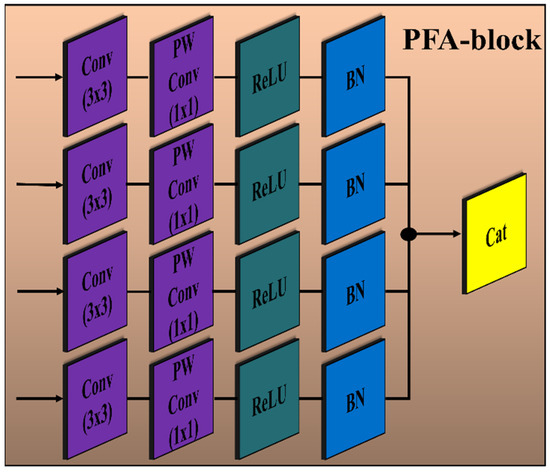
Figure 3.
Architecture of the proposed PFA block of PFA-Net. Convolution layer (Conv) with filter size (3 × 3); pointwise convolution layer (PW Conv) with filter size (1 × 1); batch normalization layer (BN); rectified linear unit layer (ReLU); concatenation layer (Cat).
The details of the layer-wise architecture of the PFA blocks (PFA-block1, -block2, -block3, -block4) are presented in Table 4. Initially, PFA-block1 in the encoder module of PFA-Net was fed with a tensor of size 76 × 76 × 64 to eliminate redundant information from low-level features. In PFA-block1, four Conv and pointwise Conv layers with filter sizes of 3 × 3 and 1 × 1, respectively, generate an output tensor of size 76 × 76 × 320 and 76 × 76 × 256, respectively. To normalize and introduce non-linearities in the low-level features, four BN and ReLU layers were applied, resulting in an output spatial tensor size of 76 × 76 × 256. Finally, the parallel low-level extracted features are concatenated through a depth-wise Conv layer into a tensor of size 76 × 76 × 1024. Similarly, PFA-block2 in the encoder module of PFA-Net was fed with a tensor of size 38 × 38 × 128 to eliminate redundant information from intermediate-level features. In PFA-block2, four Conv and pointwise Conv layers with filter sizes of 3 × 3 and 1 × 1, respectively, generate an output tensor of size 38 × 38 × 320 and 38 × 38 × 256, respectively. To normalize and introduce non-linearities in the intermediate-level features, four BN and ReLU layers were applied, resulting in an output spatial tensor size of 38 × 38 × 256. Finally, the parallel intermediate-level extracted features are concatenated through a depth-wise Conv layer into a tensor of size 38 × 38 × 1024. Similarly, PFA-block3 in the encoder module of PFA-Net was fed with a tensor of size 19 × 19 × 512 to eliminate redundant information from high-level features. In PFA-block3, four Conv and pointwise Conv layers with filter sizes of 3 × 3 and 1 × 1, respectively, generate an output tensor of size 19 × 19 × 320 and 19 × 19 × 256, respectively. To normalize and introduce non-linearities in the high-level features, four BN and ReLU layers were applied, resulting in an output spatial tensor size of 19 × 19 × 256. Finally, the parallel high-level extracted features are concatenated through a depth-wise Conv layer into a tensor of size 19 × 19 × 1024. PFA-block4 in the decoder module of PFA-Net was fed with a tensor of size 76 × 76 × 256 to leverage diverse information from different levels. In PFA-block4, four Conv and pointwise Conv layers with filter sizes of 3 × 3 and 1 × 1, respectively, generate an output tensor of size 76 × 76 × 320 and 76 × 76 × 256, respectively. Finally, the parallel-extracted features are concatenated through a depth-wise Conv layer into a tensor of size 76 × 76 × 1024, which is upsampled to an input image size of 304 × 304 × 3.
Table 4.
Details of layer-wise architecture of proposed PFA blocks of PFA-Net.
In the PFA-Net architecture, we strategically incorporate the PFA block within both the encoder and decoder frameworks by performing an ablation study, as presented in Section 4. The encoder extracts high-level features from the input data, while the decoder reconstructs the segmented output. By integrating the PFA block at multiple appropriate stages within this framework, the network can effectively leverage its feature extraction capabilities at various levels. Specifically, we integrated the PFA block at a low level in the encoder module to exploit low-level features, such as boundaries and edges of small-region tumors, especially for ET (enhancing tumor). Subsequently, we integrated the PFA block at an intermediate level in the encoder module to exploit intermediate-level features such as the shape of the BT. Finally, we integrated the PFA block at a high level in the encoder module to exploit high-level features, such as the location and size of the BT. In the decoder module, we induced the PFA block to process and aggregate the combined information captured at various levels in the encoder module, to ensure that the decoder module had access to a diverse range of information, including fine-grained details and a high-level context. This generates more accurate, detailed, and visually appealing outputs.
We used the CE loss function [68], which is commonly used for segmentation tasks, to measure the dissimilarity between the predicted probability distribution and true distribution of class labels. The mathematical definition of the CE loss function is as follows:
where denotes the total number of pixels in an image, denotes the predicted probability that pixel belongs to the foreground class, and denotes the true label of pixel .
4. Experimental Results
4.1. Experimental Dataset
As explained in Section 3.1, the proposed model was evaluated using two BT datasets from BraTS-2020 [9,22,23] as Dataset-1, and the brain tumor progression dataset [64,65] as Dataset-2. For the homogeneous dataset analysis, a five-fold cross-validation was performed using Dataset-1. Dataset-1 consisted of 369 patients, including 293 diagnosed with HGG and 76 with LGG, with four modalities including post-contrast T1-weighted (T1ce), T1, T2, and Flair. We used the T1ce and Flair modalities for their rich visual representations of tumor regions compared to other modalities. This rich dataset has been instrumental in advancing the research and development of CAD (computer-aided diagnostic) frameworks for BT segmentation. Dataset-1 is a combination of different structures of MRI BT, including gadolinium-enhancing (ET), peritumoral edema (ED), necrotic core (NCR), and non-enhancing core (NET). The diffused, irregular, and nonspecific enhancement of ET, the varying distribution and heterogeneity of ED and NCR, and coexistence of NET with ET make segmentation more challenging. The annotations of this dataset for training data are publicly accessible, whereas the annotations for test trials are not disclosed. Examples from Dataset-1 are shown in Figure 4.
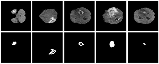
Figure 4.
Examples of brain tumor scans in the first row, with corresponding segmentation masks in the second row from Dataset-1.
To analyze heterogeneous datasets, the PFA-Net trained on Dataset-1 was applied to the entire Dataset-2 for testing. This dataset contained the MRI scans of 20 patients diagnosed with primary glioblastoma. Each patient’s data comprised two MRI examinations, totaling 8798 scans. Examples from Dataset-2 are shown in Figure 5.
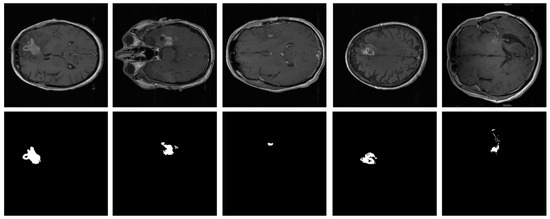
Figure 5.
Examples of brain tumor scans in the first row, with corresponding segmentation masks in the second row from Dataset-2.
4.2. Environmental Setup, Pre-Processing, and Training
All experiments, including the homogeneous and heterogeneous dataset analyses, were conducted using an Intel (R) core (TM) i5-2320 CPU@3GHz with 16 GB RAM. The experiments used an NVIDIA GeForce GTX 1070 GPU with 8 GB of graphical memory (NVIDIA GeForce 10 Series, accessed on 26 August 2023) [69]. On a Windows 10 operating system, PFA-Net was developed using MATLAB R2021b (MATLAB 2021b, accessed on 26 August 2023) [70]. A stochastic gradient descent optimizer, utilizing a 0.001 learning rate, was employed to train the PFA-Net in both homogeneous and heterogeneous dataset analysis experiments. A minibatch of size 10 was used for both homogeneous and heterogeneous dataset analyses. The default hyperparameter settings from MATLAB R2021b were used for all other parameters.
Due to the limited availability of hardware resources and to avoid complexity, we adopted a simplification approach by extracting slices from the volumetric medical imaging data, resulting in 2D grayscale images. These images were then downsampled to a resolution of 304 × 304 pixels. In total, we obtained 57,195 images from the medical data of 369 patients. Additionally, to ensure consistency and comparability across the dataset, we performed intensity normalization using Z-score normalization. This normalization technique standardizes the intensity values of the grayscale images to have a mean of 0 and a standard deviation of 1, thereby reducing the influence of variations in intensity levels across different images. Z-score normalization is commonly used as a pre-processing step in medical imaging analysis to enhance the interpretability and robustness of the data.
Dataset-1 was divided into ratios of 70%, 10%, and 20% for training, validation, and testing, respectively, based on a five-fold cross-validation. To avoid underfitting or overfitting problems, a validation dataset comprising 10% of Dataset-1 was used in the homogeneous dataset analysis. Figure 6 illustrates the training and validation losses, as well as the accuracies of PFA-Net for homogeneous dataset analysis with three segmentation masks (ET, TC, and WT) of Dataset-1 and heterogeneous dataset analysis with the segmentation mask of Dataset-2. The convergence can be observed in Figure 6, and both loss and accuracy show that our model trained well and did not suffer from overfitting during training. This shows that the PFA-Net learns to generalize BT (brain tumor) patterns from the training data. Regarding the analysis of the heterogeneous dataset, we only present the training losses/accuracies graphs in Figure 6, because we trained PFA-Net with the complete Dataset-1 and subsequently tested it with the complete Dataset-2.
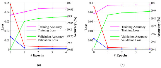
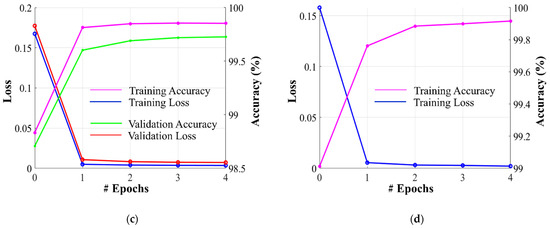
Figure 6.
Graphs depicting training/validation losses/accuracies of proposed PFA-Net for homogeneous dataset analysis with three segmentation masks: (a) ET mask, (b) TC mask, (c) WT mask, and (d) for heterogeneous dataset analysis.
4.3. Evaluation Metrics and Fractal Dimension Estimation
The DS and intersection over union (IoU) are widely used metrics in medical image segmentation, owing to their ability to quantify the overlap between segmented regions and the ground truth, which is of paramount importance in medical diagnosis and treatment planning [71]. Mathematically, the DS (Dice score) and IoU are defined as follows:
where TP stands for true positive pixels (correctly segmented as positive in both the prediction and ground truths). FP denotes the number of false-positive pixels (incorrectly segmented as positive in the prediction but not in the ground truth). FN denotes the number of false-negative pixels (incorrectly segmented as negative in the prediction but positive in the ground truth).
Fractals are complex shapes with self-similarity, defying traditional geometry rules [72] The FD (fractal dimension) quantifies complexity, revealing whether a structure is concentrated or dispersed. In our study, PFA-Net outputs predicted binary masks for four distinct types of BTs, where the FD can vary between 1 and 2, reflecting the complexity of these predictions. Within this range, FD encompasses a broad spectrum of representations for binary images, with higher values indicating greater shape complexity. By employing the box-counting technique [73], we compute the FD of BTs. If N denotes the number of boxes evenly dividing the BT, and ϵ represents the scaling factor of the box, we can calculate the FD as follows:
where FD ∈ [1,2], and for all ϵ > 0, there exists a N(ϵ). The pseudocode for estimating the FD of the generated BTs of PFA-Net using the box-counting method is provided in Algorithm 1.
| Algorithm 1: The pseudocode for estimation of fractal dimension. |
| Input: Is: input is the generated output of PFA-Net Output: fractal dimension (FD) 1: Set the maximum box size and make its dimensions powers of 2 e = 2^[log(max(size(Is))/log2] 2: Pad the Is to make its dimension equal to e if size(Is) < size(e) pad(Is) = e end 3: Pre-allocate the number of boxes n = zeros(1, e +1) 4: Compute number of boxes ‘N(e)’ containing at least one BT pixel n(e + 1) = sum(I(:)) 5: While e > 1: a. Reduce box size: e = e/2 b. Recalculate N(e) 6: Compute log(N(e)) and log(1/e) for each ‘e’ 7: Fit line to [(log(1/e), log(N(e)] using least squares 8: Fractal dimension is slope of line Return FD |
4.4. Testing Results of Homogeneous Dataset Analysis
4.4.1. Ablation Studies
We performed four ablation studies on the proposed PFA-Net based on a novel PFA block with a homogeneous dataset analysis. In the first ablation study, we considered the importance of using the optimum number of PFA blocks to obtain the maximum performance results at the cost of the learning parameters. In the second ablation study, we explored the importance of the presence of a PFA block within the decoder module by leveraging information from different levels (low, intermediate, and high) of the encoder module. The third ablation study was specifically that of the PFA block to control the number of parameters within the PFA block. In the last ablation study, we performed experiments using different loss functions. We divided the first ablation study into four cases based on the use of varying numbers of PFA blocks within the PFA-Net architecture, as listed in Table 5. Specifically, the first case involved the exclusion of any PFA blocks, while the fourth case involved all four PFA blocks. The intermediary cases, two and three, were further subdivided based on different configurations involving the use of two and three PFA blocks, respectively. The different cases of the first ablation study are listed in Table 5, as follows:
Table 5.
Performance analysis of novel PFA blocks in PFA-Net for homogeneous dataset analysis (ablation study) (Unit: %).
- (1)
- Absence of PFA block.
- (2a)
- PFA-block1 at low level of encoder and PFA-block2 at intermediate level of encoder.
- (2b)
- PFA-block3 at high level of encoder and PFA-block4 in decoder.
- (2c)
- PFA-block2 at intermediate level of encoder and PFA-block4 in decoder.
- (2d)
- PFA-block1 at low level of encoder and PFA-block3 at high-level of encoder.
- (3a)
- PFA-block2 at the intermediate level of the encoder, PFA-block3 at the high-level of the encoder, and PFA-block4 in the decoder.
- (3b)
- PFA-block1 at low encoder levels, PFA-block2 at intermediate encoder levels, and PFA-block3 at high encoder levels.
- (4)
- PFA-block1 at the low level of the encoder, PFA-block2 at the intermediate level of the encoder, PFA-block3 at the high level of the encoder, and PFA-block4 at the decoder level.
In the absence of PFA blocks for the first case, we evaluated the performance metrics by analyzing a homogeneous dataset, which established the baseline results. In the second case, involving the inclusion of two PFA blocks, we assessed the performance metrics by introducing PFA blocks at two different levels within the architecture. In this case, the segmentation performance increased to 1.2%, 0.56%, 1.01%, and 0.74 of DS values and 1.39%, 0.73%, 1.2%, and 0.92% of IoU for cases 2a, 2b, 2c, and 2d, respectively, compared with the baseline results, as indicated in Table 5. In the third case, involving the inclusion of three PFA blocks, we assessed the performance metrics by introducing PFA blocks at three different levels within the architecture. In this scenario, the segmentation efficacy increased to 2% and 1.56% of DS and 2.36% and 1.82% of IoU for cases 3a and 3b, respectively, compared to the baseline results, as indicated in Table 5. Finally, in the presence of all four PFA blocks for the fourth case, the performance results increased by 2.99% for DS and 3.62% for IoU, compared to the baseline results, as shown in Table 5. Furthermore, we conducted a t-test [74] to assess the disparity between the proposed PFA-Net and the baseline model. The PFA-Net demonstrated enhanced performance compared with the base model [66], with a 99% confidence score, resulting in an average p-value of 0.0009 (p < 0.01). This ablation study demonstrated a gradual enhancement in segmentation performance results with the progressive inclusion of novel PFA blocks.
We divided the second ablation study into four cases based on fixing the PFA block in the decoder module and varying the position of the PFA blocks within the encoder module of the PFA-Net architecture, to demonstrate the importance of the presence of the PFA block in the decoder module. The four cases in the second ablation study, listed in Table 6, are as follows.
Table 6.
Performance analysis of fixed PFA block in the decoder module of PFA-Net for homogeneous dataset analysis (ablation study) (Unit: %).
- (1)
- PFA-block1 at low level of encoder and PFA-block4 in decoder.
- (2)
- PFA-block2 at intermediate level of encoder and PFA-block4 in decoder.
- (3)
- PFA-block3 at high level of encoder and PFA-block4 in decoder.
- (4)
- PFA-block1 at the low level of the encoder, PFA-block2 at the intermediate level of the encoder, PFA-block3 at the high level of the encoder, and PFA-block4 at the decoder level.
The performance results of these four cases were compared with the baseline results from the first ablation study. In the first case, which involved incorporating the PFA block at a low level of the encoder, the performance improvement increased to 0.91% in DS and 1.04% in IoU compared with the baseline results, as indicated in Table 6. In the second case, which involved incorporating the PFA block at the intermediate level of the encoder, the performance improvement increased to 1.01% in DS and 1.2% in IoU compared with the baseline results, as listed in Table 6. In the third case, which involved incorporating the PFA block at a high level of the encoder, the performance improvement increased to 0.56% in DS and 0.73% in IoU compared with the baseline results, as indicated in Table 6. Finally, in the fourth case, involving all three PFA blocks at low, intermediate, and high levels of the encoder, the performance results increased by 2.99% for DS and 3.62% for IoU, compared with the baseline results, as indicated in Table 6. This ablation study demonstrates that the decoder module has access to a diverse range of information, including fine-grained details and high-level contexts.
In our third ablation study, we analyzed the configuration of the PFA block and aimed to control the number of parameters contained within a PFA block at the trade-off point for overall performance. Notably, our investigation revealed that the optimum performance results were achieved with a configuration of four parallel Conv and BN layers within the PFA block, as indicated in Table 7. This particular configuration is a baseline for analyzing the PFA block. When we deviated from this configuration by either increasing or decreasing the number of layers, the performance was degraded. For instance, when we incorporated three parallel Conv and BN layers within the PFA block, the parameter count decreased to 3.33 M compared to the baseline parameters. However, this reduction in parameters also led to a decrease in the performance results, with a 1.29% decrease in DS and a 1.61% decrease in IoU compared to the baseline configuration results, as indicated in Table 7. Similarly, when we expanded upon the baseline configuration by implementing five parallel Conv and BN (batch normalization) layers within the PFA block, the parameter count increased to 3.33 M, but this change also resulted in a 2.07% decrease in DS and a 2.55% decrease in IoU compared with the baseline configuration results, as shown in Table 7. We conclude that the configuration featuring four layers demonstrates an optimal balance between learnable parameter count and performance outcomes.
Table 7.
Analysis of number of learnable parameters and configuration of PFA block as ablation study.
We evaluated the performance of our PFA-Net using various loss functions and compared it with our chosen CE loss function. Table 8 presents the quantitative results of the proposed PFA-Net with a homogeneous dataset analysis using CE, weighted cross-entropy (WCE), and Dice loss (DL). It is evident from Table 8 that the segmentation performance of the proposed PFA-Net using CE is significantly superior to using WCE and DL. Specifically, the performance results of the proposed PFA-Net using CE were 9.53% and 11.96% higher in terms of DS and IoU, respectively, compared to using WCE. Similarly, the performance results of the proposed PFA-Net using CE were 3% and 4.07% higher in terms of DS and IoU, respectively, compared to using DL. CE loss proves to be a simple yet effective choice for segmentation due to its focus on binary classification (tumor and background) and efficient computation. Though WCE and DL focus more on the class imbalance, our network was unable to tune optimum weights for these losses.
Table 8.
Performance analysis of different loss functions with TC mask as ablation study.
4.4.2. Comparisons with State-of-the-Art Methods
We performed a comprehensive comparative analysis of the performance of PFA-Net, an automated diagnostic screening method for three different types of BT (ET, TC, and WT), in relation to various recent CAD methods, as presented in Table 9, Table 10 and Table 11. Existing methods focusing on BT segmentation utilize DS evaluation metrics, which are regarded as the primary performance evaluation metrics for medical images segmentation [75]. Therefore, for a fair comparison, we evaluated the results based on this metric and compared them with those of the previous CAD methods. The annotations of the BraTS-2020 dataset for the training data are publicly accessible, whereas the annotations for the validation and test trials are not disclosed; therefore, the proposed methodology was developed and evaluated based on training data, and the results were compared with those of other methods that relied on training data for a fair comparison. Our proposed PFA-Net demonstrated superior performance in terms of quantitative performance in comparison with previously designed CAD methods for the segmentation of all three types of BT, including ET (enhancing tumor), TC (tumor core), and WT (whole tumor). For example, in the case of ET, our proposed model outperforms all the baseline models and attains the first position with a significant margin of a 1.24% increment in DS from the second-ranked method [42], as listed in Table 9.
Table 9.
A comparative performance analysis of the proposed PFA-Net with existing CAD methods for the segmentation of enhancing tumor (ET) (Unit: %).
Table 10.
A comparative performance analysis of the proposed PFA-Net with existing CAD methods for the segmentation of tumor core (TC) (Unit: %).
Table 11.
A comparative performance analysis of the proposed PFA-Net with CAD methods for the segmentation of whole tumor (WT) (Unit: %).
Figure 7 displays the qualitative results of ET segmentation performed using the proposed PFA-Net within a homogeneous dataset. In the case of TC segmentation, our proposed model outperforms all baseline models and attains the first position with a significant margin of 1.22% from the second-ranked method [42], as indicated in Table 10. Figure 8 displays the qualitative results of the TC segmentation performed by the proposed PFA-Net within a homogeneous dataset. In the case of WT segmentation, our proposed model outperforms all baseline models and attains the first position with a significant margin of 0.42% from the second-ranked method [45], as listed in Table 11. Figure 9 displays the qualitative results of the WT segmentation performed by the proposed PFA-Net within a homogeneous dataset.
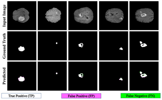
Figure 7.
Qualitative results of the proposed PFA-Net for the segmentation of enhancing tumor (ET).

Figure 8.
Qualitative results of the proposed PFA-Net for the segmentation of tumor core (TC).
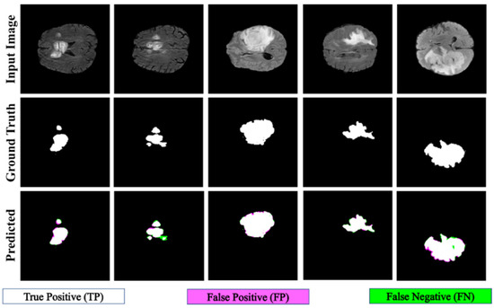
Figure 9.
Qualitative results of the proposed PFA-Net for the segmentation of whole tumor (WT).
A comparative study of the homogeneous dataset analysis, as presented in Table 9, Table 10 and Table 11, provides valuable insights into the performance of various CAD methods. It was concluded that different CAD methods tend to excel in the diagnosis of one type of tumor, while exhibiting lower performance for other types. This limitation suggests that these methods may have a specialization but lack the ability to generalize effectively across all tumor types. In contrast, our proposed PFA-Net not only excels in diagnosing one specific type of tumor but also achieves optimal performance for all three types of tumors (ET, TC, and WT) and surpasses the performance of all state-of-the-art methods.
4.5. Testing Results of Heterogeneous Dataset Analysis
We performed a comprehensive comparative analysis of the performance of PFA-Net, an automated diagnostic screening method for heterogeneous dataset analysis, in relation to various recent CAD methods, as presented in Table 2 and Table 12. A previous method [19] used a pre-processing step to enhance the performance of the heterogeneous dataset analysis. Some methods [63] do not consider a complete heterogeneous dataset analysis. Our proposed PFA-Net demonstrates superior performance compared with previous methods for the analysis of a completely heterogeneous dataset without requiring a pre-processing technique.
Table 12.
Comparative performance analysis of proposed PFA-Net with existing CAD methods for heterogeneous dataset analysis. Million (M); Megabytes (MB); Seconds (s).
Table 12 presents a comparison of the performance of PFA-Net in relation to various state-of-the-art methods [18,19,44,66,76,77,78,79] for analyzing the heterogeneous dataset. The proposed method outperforms the second-ranked method [19] with DS and IoU performance gains of 64.58% and 59.03%, respectively, as listed in Table 12. Additionally, our method is efficient in terms of the number of parameters, testing elapsed time, and memory usage compared to the second-best method [19], as shown in Table 12. Specifically, the parameters of the proposed PFA-Net are 19.49 M less than those of MDFU-Net (i.e., 31.48 M [Proposed] << 50.97 M [MDFU-Net]). The average processing time of one BT scan is 0.77 s less than that of MDFU-Net (i.e., 1.53 s [Proposed] < 2.3 s [MDFU-Net]), and the average memory used by the proposed PFA-Net is 219.11 megabytes (MB) less than that of MDFU-Net (i.e., 318.69 MB [Proposed] << 537.8 MB [MDFU-Net]), as shown in Table 12. However, the computational complexity of the proposed PFA-Net is high in terms of gigaflops floating-point operations per second (GFLOPS) compared to the second-best method [19] (i.e., 126.85 GFLOPS [Proposed] > 105.85 GFLOPS [MDFU-Net]). This complexity is attributed to the intensive computations required for parallel feature extraction by the novel PFA block. Nevertheless, the proposed PFA-Net ranked first in terms of segmentation accuracy compared to all other methods, as indicated in Table 12. Figure 10 shows the qualitative results obtained using the proposed PFA-Net on a heterogeneous dataset.
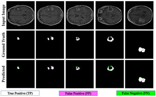
Figure 10.
Qualitative results of proposed PFA-Net for heterogeneous dataset analysis.
4.6. FD Estimation for BTs
We apply the box-counting method to calculate the FD (fractal dimension) for analyzing the BT (brain tumor) images from Dataset-1 and Dataset-2 for better characterization, as illustrated in Figure 11, Figure 12, Figure 13 and Figure 14. In addition, we calculate the correlation coefficient (C) value and R2 for both datasets. The first row of Figure 11, Figure 12, Figure 13 and Figure 14 displays the predicted mask generated by PFA-Net, while the second row depicts the count of boxes (N(ϵ)) for various box sizes (ϵ). The third row of Figure 11, Figure 12, Figure 13 and Figure 14 is derived from Equation (11), with the slope of the line providing the FD estimation of BTs. Table 13 presents the results of FD analysis, along with the C value and R2, for different tumor types, including ET, TC, WT, and the heterogeneous dataset analysis of Figure 11, Figure 12, Figure 13 and Figure 14.
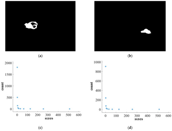
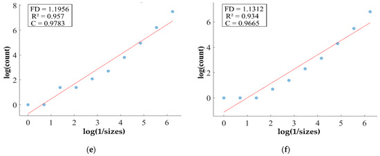
Figure 11.
FD analysis for the segmentation of ET: The first row displays the generated ET mask by PFA-Net. The second row illustrates the various sizes of the box and their corresponding counts. In the third row, the FD value calculated by Equation (11) is shown, along with R2 and C values for the ET mask. (c,e) are calculated from the image of (a), whereas (d,f) are calculated from the image of (b).
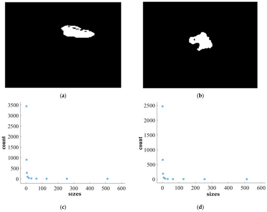
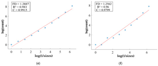
Figure 12.
FD analysis for the segmentation of TC: The first row displays the generated TC mask by PFA-Net. The second row illustrates the various sizes of the box and their corresponding counts. In the third row, the FD value calculated by Equation (11) is shown, along with R2 and C values for TC mask. (c,e) are calculated from the image of (a), whereas (d,f) are calculated from the image of (b).
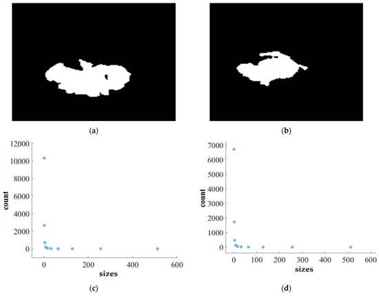
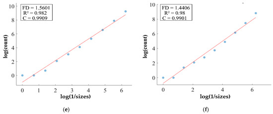
Figure 13.
FD analysis for the segmentation of WT: The first row displays the generated WT mask by PFA-Net. The second row illustrates the various sizes of the box and their corresponding counts. In the third row, the FD value calculated by Equation (11) is shown, along with R2 and C values for WT mask. (c,e) are calculated from the image of (a), whereas (d,f) are calculated from the image of (b).
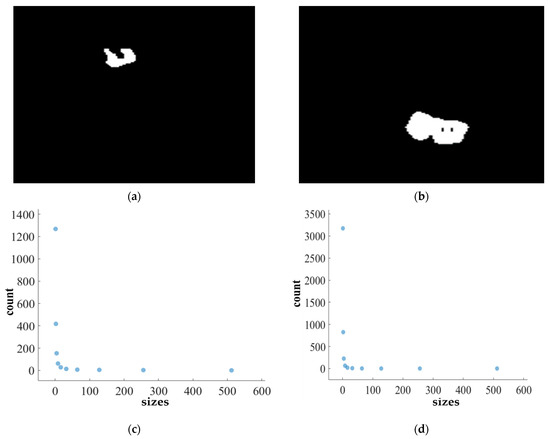
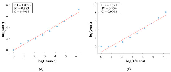
Figure 14.
FD analysis for the segmentation of heterogeneous dataset analysis: The first row displays the generated heterogeneous dataset mask by PFA-Net. The second row illustrates the various sizes of the box and their corresponding counts. In the third row, the FD value calculated by Equation (11) is shown, along with R2 and C values for heterogeneous dataset. (c,e) are calculated from the image of (a), whereas (d,f) are calculated from the image of (b).
Figure 11, Figure 12, Figure 13 and Figure 14 present a detailed analysis of FD estimation for the segmentation of both homogeneous and heterogeneous datasets. For example, Figure 11 provides the FD analysis for the segmentation of ET using the PFA-Net, illustrating two separate samples. The first row of Figure 11 displays the generated ET masks by PFA-Net. Each mask is a binary image where the white region represents the segmented tumor. These masks are essential for the subsequent FD analysis, as they provide the structural data needed to estimate the FD. The second row of Figure 11 illustrates the various sizes of the boxes and their corresponding counts calculated by Algorithm 1. This visualization is fundamental to the box-counting method used for estimating the FD. By covering the ET masks with boxes of different sizes and counting the number of boxes that intersect with the tumor, we obtain the necessary data for calculating the FD. The third row presents the FD values calculated using Equation (11), along with the R2 and C values for each ET mask.
The FD values indicate the complexity and irregularity of the ET shapes. A higher FD value suggests more intricate and irregular shapes, while a lower value indicates simpler shapes. The first sample of the ET mask (Figure 11a) has a higher FD value (1.1956) compared to the second sample (Figure 11b), which has an FD value of 1.1312, suggesting that the ET of the first sample is more complex and irregular. Higher R2 values closer to 1 signify a better fit of the model to the data. The high R2 values for Figure 11a (0.957) and Figure 11b (0.934) indicate a strong linear relationship in the log–log plot of box sizes and their counts. This high degree of fit suggests that the FD values are reliable measures of the complexity of ET. Similarly, higher C values closer to 1 signify a stronger linear relationship between the variables. Higher C values for Figure 11a (0.9783) and Figure 11b (0.9665) demonstrate a strong relationship between the size of the boxes and their counts.
Higher FD values indicate greater complexity and irregularity in the morphology of the BTs. For example, in Table 13, the highest FD value of 1.5601 is observed in the WT, suggesting significant irregularities in these areas. This highlights the importance for medical experts to conduct thorough analyses of the morphometric properties of the WT. R2 values range from 0.934 to 0.983, indicating the goodness of fit of the linear regression model used to estimate the FD values, as shown in Table 13. Higher R2 values closer to 1 signify a better fit of the model to the data. Furthermore, the C value indicates the strength and direction of the linear relationship between the FD values and the actual BT morphology. Higher C values closer to 1 signify a stronger linear relationship between the variables.
The FD values presented in Table 13 offer insights into the complexity and irregularity of different tumor types. By examining two samples of each tumor type, we can assess their complexity. For the ET samples, with FD values of 1.1956 and 1.1312, there is a moderate level of complexity and irregularity in their shapes. In contrast, the TC samples exhibit FD values of 1.2887 and 1.2562, indicating a slightly higher complexity compared to the ET samples. The higher severity observed in the TC sample is attributed to its composition, which includes ET as well as NCR and NET components. The WT samples exhibit FD values of 1.5601 and 1.4406, indicating the most intricate and irregular shapes among the three tumor types of Dataset-1. The high severity observed in the WT sample is attributed to its composition, which includes TC as well as ED components. These FD values provide crucial insights into the structural characteristics of each tumor type, which are useful in tumor pathology. For the heterogeneous dataset analysis, we obtained different FD values (1.0776 and 1.3711).
The FD (fractal dimension) parameter serves as a crucial metric for understanding the intricacies of BT shapes, providing detailed insights for both homogeneous and heterogeneous datasets. In homogeneous dataset analysis, FD values provide detailed assessments of individual tumor types, with moderate values in ET samples indicating a moderate level of complexity and irregularity, slightly higher values in TC samples suggesting elevated complexity, and the highest values in WT samples representing the most intricate and irregular shapes. On the other hand, for heterogeneous data analysis, FD values offer a broader perspective, capturing the overall complexity of the dataset characterized by the presence of different tumor types and compositions. The variability in FD values across heterogeneous samples signifies the diverse nature of BT shapes within the dataset, with lower values indicating less complexity and irregularity, and higher values reflecting increased complexity and variability, likely due to the inclusion of various BT types or compositions. Overall, FD serves as a measure of irregularity [80], with higher FD values often indicating more intricate and irregular tumor shapes, thereby guiding medical experts to predict tumor malignancy and prioritize analysis for treatment decisions and enhanced patient care [81]. Moreover, it allows researchers to assess and compare the intricacy of tumor shapes within each dataset and across different datasets, aiding in understanding tumor behavior and composition.
5. Discussion
CAD (computer-aided diagnostic) tools are typically tailored for specific applications in medical diagnosis. Designing a general-purpose tool for clinical applications is challenging because of the diverse structural features of diagnoses, variations in medical radiography equipment, and substantial inter-patient variance in data. To address this problem, we introduce a novel DL-based network for parallel feature aggregation, specifically designed for the analysis of heterogeneous datasets. Although the performance results are low (DS of 64.58%), they surpassed the previous CAD methods, with 19.49 M (million) parameters and 219.11 MB (megabytes) memory less than the approach by [19], specifically designed for heterogeneous dataset analysis (Table 12).
To demonstrate the substantial disparity (statistical significance) between the proposed model and the base model [66], we conducted a t-test [74] and calculated Cohen’s d value [82] for all three tumors in the homogeneous dataset analysis. Table 14 and Figure 15 show the average performance gain and p-value of the proposed PFA-Net compared with the base model for three tumors, including ET (enhancing tumor), TC (tumor core), and WT (whole tumor). In detail, the proposed PFA-Net gained 2.99% in DS (Dice score) value for ET compared to the base model, with a p-value of 0.0009 (99% confidence level) and Cohen’s d value of 1.3267 (large effective size). For TC, the proposed PFA-Net gained 4.31% in DS value compared to the base model, with a p-value of 0.0052 (99% confidence level) and Cohen’s d value of 1.0012 (large effective size). For WT, the proposed PFA-Net gained 1.64% in DS value compared to the base model, with a p-value of 0.003 (99% confidence level) and Cohen’s d value of 2.4371 (large effective size). These findings suggest a significant difference between the proposed and base models, as depicted in Table 14 and Figure 15.
Table 14.
Performance gain and substantial disparity between proposed model and base model in terms of p-value and Cohen’s d value.
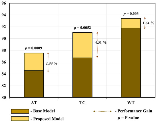
Figure 15.
Performance gain and substantial disparity between proposed model and base model.
The homogeneous dataset consisted of three diverse tumor types (ET, TC, and WT) and posed a significant challenge owing to the structural complexities arising from intra-class variations. Previous CAD methods have demonstrated excellent performance in diagnosing one tumor type, while exhibiting performance degradation when dealing with the other two. For instance, the modality-pairing 3D U-Net [42] is the second-best method for the segmentation of ET and TC (Table 9 and Table 10). However, its performance degrades when applied to WT segmentation, dropping to the fourth position in this particular scenario. Similarly, the triplanar U-Net [45] was the second-best method for WT segmentation (Table 11). However, its performance degraded when applied to the segmentation of ET and TC, decreasing to the fourth and twelfth positions, respectively (Table 9 and Table 10). Similarly, other CAD methods have variable performance results for different types of tumors. In contrast, our proposed model (PFA-Net) exhibits superior performance across all three tumor types (ET, TC, and WT). Specifically, our PFA module leverages the localized radiomic contextual spatial features of BT at low, intermediate, and high levels, aggregating them in parallel. This approach contributes to performance improvements across all three tumor types, particularly ET.
The proposed PFA-Net demonstrated superior qualitative visual results for both homogeneous and heterogeneous dataset analysis in a challenging environment. Figure 16 illustrates the correct segmentation results for homogeneous dataset analysis with three segmentation masks, including ET, TC, and WT, and for heterogeneous dataset analysis. In detail, the first row of Figure 16 visually highlights the challenges in analyzing BT scans, such as a minute tumor in the case of ET, having only the border edge of tumors for TC, the amalgamation of tumor features with background features for WT, and the enhancement of edges by tumor-like features in the heterogeneous dataset analysis. Despite these challenges, PFA-Net demonstrates superior performance for all cases. However, the performance of PFA-Net is constrained due to diffuse and irregular characteristics, non-specific enhancement, diverse distribution, heterogeneity, and the coexistence of different tumor components, as shown in Figure 17. This indicates that while PFA-Net excels in certain scenarios, there are specific tumor configurations that present challenges to its overall performance.
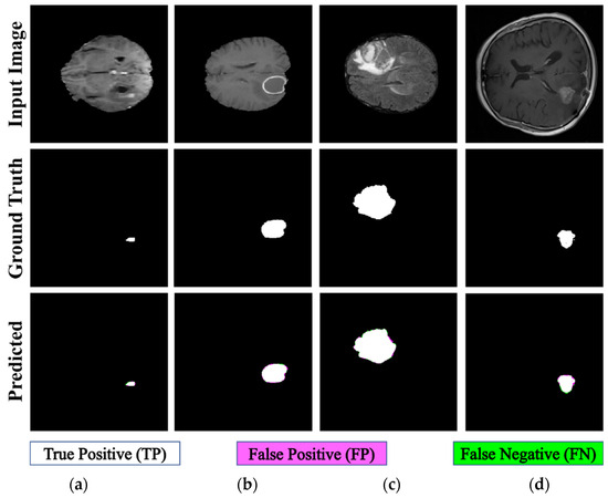
Figure 16.
Examples of correct segmentation for homogeneous dataset analysis with three segmentation masks: (a) ET mask, (b) TC mask, (c) WT mask, and (d) for heterogeneous dataset analysis.

Figure 17.
Examples of incorrect segmentation for homogeneous dataset analysis with three segmentation masks: (a) ET mask, (b) TC mask, (c) WT mask, and (d) for heterogeneous dataset analysis.
For a detailed analysis, we extracted gradient-weighted class activation maps (Grad-CAM) [83] from the four PFA blocks, which revealed the distinctive features of the BT scans as a reddish color. The key role of the novel PFA blocks in homogeneous and heterogeneous dataset analyses are shown in Figure 18. As depicted in Figure 18, the evolution of tumor regions becomes increasingly focused and discernible as the network progresses through these different blocks, confirming that our proposed model can extract important features for the accurate segmentation of tumor regions. Ultimately, we achieved the precise localization of tumor regions marked as “1” and background regions marked as “0”.
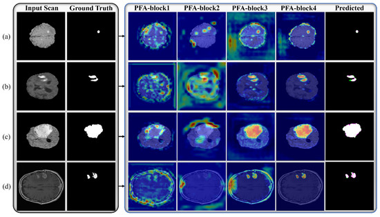
Figure 18.
Visual representation of Grad-CAM results extracted from various PFA blocks of PFA-Net for homogeneous dataset analysis: (a) ET mask, (b) TC mask, (c) WT mask, and (d) for heterogeneous dataset analysis.
6. Conclusions
This study addressed the challenge of pixel-based segmentation in both homogeneous and heterogeneous environments. We introduced a parallel feature aggregation-based module that relies on multiple-branch feature extraction operations to learn discriminative information from BT scans in parallel and aggregate them. Specifically, we leverage these three modules at various levels in the encoder of the proposed segmentation framework to obtain spatial semantic information at various levels, and one module is integrated into the decoder of the proposed segmentation framework to process the various levels of information from the encoder. Finally, incorporating an FD estimation method into our system yields valuable insights into the distributional characteristics of BTs, especially for WT, thereby enriching the comprehensiveness of our approach.
Our proposed method was applied to the segmentation of different types of BT scans from different datasets, and the results demonstrated its superiority over previous CAD methods in terms of DS values of 87.54%, 91.02%, and 93.42% for a homogeneous dataset analysis and 64.58% for a heterogeneous dataset analysis, with 19.49 M fewer learning parameters than those of the previous method. In addition, a statistical analysis confirmed a significant difference in segmentation accuracy between our model and the base model, with p-values of 0.0009, 0.0052, and 0.003 for ET, TC, and WT, respectively, and Cohen’s d values of 1.3267, 1.0012, and 2.4371, for ET, TC, and WT, respectively, as shown in Table 14 and Figure 15.
Despite achieving the optimum DS using our proposed method for homogeneous and heterogeneous datasets, this study has some limitations. The number of parameters was increased by 3.33 M following the addition of each PFA block. In future, the parameters will be reduced by introducing a dilation operation into the PFA blocks. Incorrect segmentation occurred in both homogeneous and heterogeneous dataset analyses, as depicted in Figure 17. The first row of Figure 17 visually underscores the challenges in analyzing BT scans, attributed to diffuse and irregular characteristics, non-specific enhancement, and diverse distribution. Furthermore, the second row of Figure 17 illustrates that the small ground truth masks of tumors are dispersed, posing an additional challenge for our model, which did not accurately segment them. In future, we will apply pre-processing methods to address these challenges. Moreover, because the segmentation performance for heterogeneous dataset analysis is limited compared with that for a homogeneous dataset analysis, the performance can be improved by using a balanced heterogeneous dataset.
While a box-counting algorithm was employed for FD estimation in our study, it is worth noting that other fractal-based methods could potentially be embedded within the proposed framework. Fractal analysis offers a versatile approach for quantifying the complexity and irregularity of signals, including those derived from medical imaging data such as brain tumors. Therefore, exploring alternative fractal-based methods could offer additional insights and potentially enhance the robustness of our framework. Some examples of other fractal-based methods that could be considered include the Higuchi fractal dimension [84], multifractal analysis [85], and fractal-derived texture analysis [86]. Each of these methods has its strengths and limitations, and incorporating them into future iterations of our framework could contribute to a more comprehensive understanding of the fractal nature of BT. Additionally, exploring the potential synergies between different fractal-based methods may lead to further improvements in accuracy and reliability.
Author Contributions
Methodology, Writing—original draft, H.S.; Conceptualization, N.U.; Data curation, J.S.H.; Investigation, S.G.K.; Resources, D.C.L.; Visualization, S.Y.J.; Supervision, Writing—review and editing, K.R.P. All authors have read and agreed to the published version of the manuscript.
Funding
This research was supported by the Ministry of Science and ICT (MSIT), Korea, under the Information Technology Research Center (ITRC) support program (IITP-2024-2020-0-01789) supervised by the Institute for Information and Communications Technology Planning and Evaluation (IITP).
Data Availability Statement
The proposed PFA-Net brain tumor segmentation models were made publicly available via the Github site (https://github.com/PFA-Net, accessed on 23 November 2023).
Conflicts of Interest
The authors declare no conflicts of interest.
References
- Raghavendra, U.; Gudigar, A.; Paul, A.; Goutham, T.; Inamdar, M.A.; Hegde, A.; Devi, A.; Ooi, C.P.; Deo, R.C.; Barua, P.D.; et al. Brain tumor detection and screening using artificial intelligence techniques: Current trends and future perspectives. Comput. Biol. Med. 2023, 163, 107063. [Google Scholar] [CrossRef] [PubMed]
- Louis, D.N.; Ohgaki, H.; Wiestler, O.D.; Cavenee, W.K.; Burger, P.C.; Jouvet, A.; Scheithauer, B.W.; Kleihues, P. The 2007 WHO classification of tumours of the central nervous system. Acta Neuropathol. 2007, 114, 97–109. [Google Scholar] [CrossRef] [PubMed]
- Vescovi, A.L.; Galli, R.; Reynolds, B.A. Brain tumour stem cells. Nat. Rev. Cancer 2006, 6, 425–436. [Google Scholar] [CrossRef] [PubMed]
- Miller, K.D.; Ostrom, Q.T.; Kruchko, C.; Patil, N.; Tihan, T.; Cioffi, G.; Fuchs, H.E.; Waite, K.A.; Jemal, A.; Siegel, R.L.; et al. Brain and other central nervous system tumor statistics, 2021. CA-Cancer J. Clin. 2021, 71, 381–406. [Google Scholar] [CrossRef] [PubMed]
- Cavaliere, R.; Lopes, M.B.S.; Schiff, D. Low-grade gliomas: An update on pathology and therapy. Lancet Neurol. 2005, 4, 760–770. [Google Scholar] [CrossRef]
- Robbins, M.; Greene-Schloesser, D.; Peiffer, A.; Shaw, E.; Chan, M.; Wheeler, K. Radiation-induced brain injury: A review. Front. Oncol. 2012, 2, 30551. [Google Scholar]
- de Leeuw, C.N.; Vogelbaum, M.A. Supratotal resection in glioma: A systematic review. Neuro-Oncol. 2019, 21, 179–188. [Google Scholar] [CrossRef] [PubMed]
- Barnova, K.; Mikolasova, M.; Kahankova, R.V.; Jaros, R.; Kawala-Sterniuk, A.; Snasel, V.; Mirjalili, S.; Pelc, M.; Martinek, R. Implementation of artificial intelligence and machine learning-based methods in brain–computer interaction. Comput. Biol. Med. 2023, 163, 107135. [Google Scholar] [CrossRef] [PubMed]
- Menze, B.H.; Jakab, A.; Bauer, S.; Kalpathy-Cramer, J.; Farahani, K.; Kirby, J.; Burren, Y.; Porz, N.; Slotboom, J.; Wiest, R.; et al. The multimodal brain tumor image segmentation benchmark (BRATS). IEEE Trans. Med. Imaging 2015, 34, 1993–2024. [Google Scholar] [CrossRef] [PubMed]
- Menze, B.; Isensee, F.; Wiest, R.; Wiestler, B.; Maier-Hein, K.; Reyes, M.; Bakas, S. Analyzing magnetic resonance imaging data from glioma patients using deep learning. Comput. Med. Imaging Graph 2021, 88, 101828. [Google Scholar] [CrossRef] [PubMed]
- Haider, A.; Arsalan, M.; Lee, M.B.; Owais, M.; Mahmood, T.; Sultan, H.; Park, K.R. Artificial intelligence-based computer-aided diagnosis of glaucoma using retinal fundus images. Expert Syst. Appl. 2022, 207, 117968. [Google Scholar] [CrossRef]
- Esteva, A.; Chou, K.; Yeung, S.; Naik, N.; Madani, A.; Mottaghi, A.; Liu, Y.; Topol, E.; Dean, J.; Socher, R. Deep learning-enabled medical computer vision. npj Digit Med. 2021, 4, 5. [Google Scholar] [CrossRef] [PubMed]
- Owais, M.; SikYoon, H.; Mahmood, T.; Haider, A.; Sultan, H.; Park, K.R. Light-weighted ensemble network with multilevel activation visualization for robust diagnosis of COVID-19 pneumonia from large-scale chest radiographic database. Appl. Soft Comput. 2021, 108, 107490. [Google Scholar] [CrossRef] [PubMed]
- Sultan, H.; Owais, M.; Park, C.; Mahmood, T.; Haider, A.; Park, K.R. Artificial intelligence-based recognition of different types of shoulder implants in X-ray scans based on dense residual ensemble-network for personalized medicine. J. Pers. Med. 2021, 11, 482. [Google Scholar] [CrossRef] [PubMed]
- LeCun, Y.; Bengio, Y.; Hinton, G. Deep learning. Nature 2015, 521, 436–444. [Google Scholar] [CrossRef]
- Demirhan, A.; Güler, İ. Combining stationary wavelet transform and self-organizing maps for brain MR image segmentation. Eng. Appl. Artif. Intell. 2011, 24, 358–367. [Google Scholar] [CrossRef]
- Guo, P. Brain tissue classification method for clinical decision-support systems. Eng. Appl. Artif. Intell. 2017, 64, 232–241. [Google Scholar] [CrossRef]
- Liu, D.; Sheng, N.; He, T.; Wang, W.; Zhang, J.; Zhang, J. SGEResU-Net for brain tumor segmentation. Math Biosci. Eng. 2022, 19, 5576–5590. [Google Scholar] [CrossRef] [PubMed]
- Sultan, H.; Owais, M.; Nam, S.H.; Haider, A.; Akram, R.; Usman, M.; Park, K.R. MDFU-Net: Multiscale dilated features up-sampling network for accurate segmentation of tumor from heterogeneous brain data. J. King Saud Univ.-Comput. Inf. Sci. 2023, 35, 101560. [Google Scholar] [CrossRef]
- Rehman, M.U.; Ryu, J.; Nizami, I.F.; Chong, K.T. RAAGR2-Net: A brain tumor segmentation network using parallel processing of multiple spatial frames. Comput. Biol. Med. 2023, 152, 106426. [Google Scholar] [CrossRef] [PubMed]
- Jia, Z.; Zhu, H.; Zhu, J.; Ma, P. Two-Branch network for brain tumor segmentation using attention mechanism and super-resolution reconstruction. Comput. Biol. Med. 2023, 157, 106751. [Google Scholar] [CrossRef] [PubMed]
- Bakas, S.; Akbari, H.; Sotiras, A.; Bilello, M.; Rozycki, M.; Kirby, J.S.; Freymann, J.B.; Farahani, K.; Davatzikos, C. Advancing the cancer genome atlas glioma MRI collections with expert segmentation labels and radiomic features. Sci. Data 2017, 4, 170117. [Google Scholar] [CrossRef] [PubMed]
- Bakas, S.; Reyes, M.; Jakab, A.; Bauer, S.; Rempfler, M.; Crimi, A.; Shinohara, R.T.; Berger, C.; Ha, S.M.; Rozycki, M.; et al. Identifying the best machine learning algorithms for brain tumor segmentation, progression assessment, and overall survival prediction in the BRATS challenge 2019. arXiv 2019, arXiv:1811.02629. [Google Scholar] [CrossRef]
- Havlin, S.; Buldyrev, S.; Goldberger, A.; Mantegna, R.N.; Ossadnik, S.; Peng, C.-K.; Simons, M.; Stanley, H. Fractals in biology and medicine. Chaos Solitons Fractals 1995, 6, 171–201. [Google Scholar] [CrossRef] [PubMed]
- Sabir, Z.; Bhat, S.A.; Wahab, H.A.; Camargo, M.E.; Abildinova, G.; Zulpykhar, Z. A bio inspired learning scheme for the fractional order kidney function model with neural networks. Chaos Solitons Fractals 2024, 180, 114562. [Google Scholar] [CrossRef]
- Chen, Y.; Wang, Y.; Li, X. Fractal dimensions derived from spatial allometric scaling of urban form. Chaos Solitons Fractals 2019, 126, 122–134. [Google Scholar] [CrossRef]
- Zook, J.M.; Iftekharuddin, K.M. Statistical analysis of fractal-based brain tumor detection algorithms. Magn. Reason. Imaging 2005, 23, 671–678. [Google Scholar] [CrossRef]
- Ronneberger, O.; Fischer, P.; Brox, T. U-Net: Convolutional networks for biomedical image segmentation 2015. arXiv 2015, arXiv:1505.04597. [Google Scholar] [CrossRef]
- Çiçek, Ö.; Abdulkadir, A.; Lienkamp, S.S.; Brox, T.; Ronneberger, O. 3D U-Net: Learning dense volumetric segmentation from sparse annotation 2016. arXiv 2016, arXiv:1606.06650. [Google Scholar] [CrossRef]
- Velthuizen, R.P.; Clarke, L.P.; Phuphanich, S.; Hall, L.O.; Bensaid, A.M.; Arrington, J.A.; Greenberg, H.M.; Silbiger, M.L. Unsupervised measurement of brain tumor volume on MR images. J. Magn. Reason. Imaging 1995, 5, 594–605. [Google Scholar] [CrossRef] [PubMed]
- Kamber, M.; Shinghal, R.; Collins, D.L.; Francis, G.S.; Evans, A.C. Model-based 3-D segmentation of multiple sclerosis lesions in magnetic resonance brain images. IEEE Trans. Med. Imaging 1995, 14, 442–453. [Google Scholar] [CrossRef] [PubMed]
- Gibbs, P.; Buckley, D.L.; Blackband, S.J.; Horsman, A. Tumour volume determination from MR images by morphological segmentation. Phys. Med. Biol. 1996, 41, 2437–2446. [Google Scholar] [CrossRef] [PubMed]
- Clark, M.C.; Hall, L.O.; Goldgof, D.B.; Velthuizen, R.; Murtagh, F.R.; Silbiger, M.S. Automatic tumor segmentation using knowledge-based techniques. IEEE Trans. Med. Imaging 1998, 17, 187–201. [Google Scholar] [CrossRef] [PubMed]
- Kaus, M.R.; Warfield, S.K.; Nabavi, A.; Chatzidakis, E.; Black, P.M.; Jolesz, F.A.; Kikinis, R. Segmentation of meningiomas and low grade gliomas in MRI. In Proceedings of the Second International Conference on Medical Image Computing and Computer-Assisted Intervention–MICCAI’99, Berlin, Heidelberg, 19–22 September 1999; pp. 1–10. [Google Scholar] [CrossRef]
- Warfield, S.K.; Kaus, M.; Jolesz, F.A.; Kikinis, R. Adaptive, template moderated, spatially varying statistical classification. Med. Image. Anal. 2000, 4, 43–55. [Google Scholar] [CrossRef] [PubMed]
- Mazzara, G.P.; Velthuizen, R.P.; Pearlman, J.L.; Greenberg, H.M.; Wagner, H. Brain tumor target volume determination for radiation treatment planning through automated MRI segmentation. Int. J. Radiat. Oncol. Biol. Phys. 2004, 59, 300–312. [Google Scholar] [CrossRef] [PubMed]
- Tustison, N.J.; Shrinidhi, K.L.; Wintermark, M.; Durst, C.R.; Kandel, B.M.; Gee, J.C.; Grossman, M.C.; Avants, B.B. Optimal symmetric multimodal templates and concatenated random forests for supervised brain tumor segmentation (simplified) with ANTsR. Neuroinformatics 2015, 13, 209–225. [Google Scholar] [CrossRef]
- Pinto, A.; Pereira, S.; Correia, H.; Oliveira, J.; Rasteiro, D.M.L.D.; Silva, C.A. Brain tumour segmentation based on extremely randomized forest with high-level features. In Proceedings of the 37th Annual International Conference of the IEEE Engineering in Medicine and Biology Society (EMBC), Milan, Italy, 25–29 August 2015; pp. 3037–3040. [Google Scholar] [CrossRef]
- Kikinis, R.; Pieper, S. 3D Slicer as a tool for interactive brain tumor segmentation. In Proceedings of the Annual International Conference of the IEEE Engineering in Medicine and Biology Society, Boston, MA, USA, 30 August–3 September 2011; pp. 6982–6984. [Google Scholar] [CrossRef]
- Gao, Y.; Kikinis, R.; Bouix, S.; Shenton, M.; Tannenbaum, A. A 3D interactive multi-object segmentation tool using local robust statistics driven active contours. Med. Image Anal. 2012, 16, 1216–1227. [Google Scholar] [CrossRef] [PubMed]
- Jun, W.; Haoxiang, X.; Wang, Z. Brain tumor segmentation using dual-path attention U-Net in 3D MRI images. In Proceedings of the 6th International MICCAI Brain Workshop, Lima, Peru, 4 October 2020; Springer International Publishing: Lima, Peru, 2020; pp. 183–193. [Google Scholar] [CrossRef]
- Wang, Y.; Zhang, Y.; Hou, F.; Liu, Y.; Tian, J.; Zhong, C.; Zhang, Y.; He, Z. Modality-pairing learning for brain tumor segmentation. In Proceedings of the 6th International MICCAI Brain Workshop, Lima, Peru, 4 October 2020; Springer International Publishing: Lima, Peru, 2020; pp. 230–240. [Google Scholar] [CrossRef]
- Yuan, Y. Automatic brain tumor segmentation with scale attention network. In Proceedings of the 6th International MICCAI Brain Workshop, Lima, Peru, 4 October 2020; Springer International Publishing: Lima, Peru, 2020; pp. 285–294. [Google Scholar] [CrossRef]
- Henry, T.; Carré, A.; Lerousseau, M.; Estienne, T.; Robert, C.; Paragios, N.; Deutsch, E. Brain tumor segmentation with self-ensembled, deeply-supervised 3D U-Net neural networks: A BraTS 2020 challenge solution. In Proceedings of the 6th International MICCAI Brain Workshop, Lima, Peru, 4 October 2020; Springer International Publishing: Lima, Peru, 2020; pp. 327–339. [Google Scholar] [CrossRef]
- Sundaresan, V.; Griffanti, L.; Jenkinson, M. Brain tumour segmentation using a triplanar ensemble of U-Nets on MR images. In Proceedings of the 6th International MICCAI Brain Workshop, Lima, Peru, 4 October 2020; Springer International Publishing: Lima, Peru, 2020; pp. 340–353. [Google Scholar] [CrossRef]
- Ballestar, L.M.; Vilaplana, V. MRI brain tumor segmentation and uncertainty estimation using 3D-UNet architectures. In Proceedings of the 6th International MICCAI Brain Workshop, Lima, Peru, 4 October 2020; Springer International Publishing: Lima, Peru, 2020; pp. 376–390. [Google Scholar] [CrossRef]
- Zhang, Y.; Wu, J.; Huang, W.; Chen, Y.; Wu, E.X.; Tang, X. Utility of brain parcellation in enhancing brain tumor segmentation and survival prediction. In Proceedings of the 6th International MICCAI Brain Workshop, Lima, Peru, 4 October 2020; Springer International Publishing: Lima, Peru, 2020; pp. 391–400. [Google Scholar] [CrossRef]
- Zhao, C.; Zhao, Z.; Zeng, Q.; Feng, Y. MVP U-Net: Multi-view pointwise U-Net for brain tumor segmentation. In Proceedings of the 6th International MICCAI Brain Workshop, Lima, Peru, 4 October 2020; Springer International Publishing: Lima, Peru, 2020; pp. 93–103. [Google Scholar] [CrossRef]
- Isensee, F.; Jäger, P.F.; Full, P.M.; Vollmuth, P.; Maier-Hein, K.H. nnU-Net for Brain Tumor Segmentation. In Proceedings of the 6th International MICCAI Brain Workshop, Lima, Peru, 4 October 2020; Springer International Publishing: Lima, Peru, 2020; pp. 118–132. [Google Scholar] [CrossRef]
- Isensee, F.; Jaeger, P.F.; Kohl, S.A.A.; Petersen, J.; Maier-Hein, K.H. nnU-Net: A self-configuring method for deep learning-based biomedical image segmentation. Nat. Methods 2021, 18, 203–211. [Google Scholar] [CrossRef] [PubMed]
- Awasthi, N.; Pardasani, R.; Gupta, S. Multi-threshold Attention U-Net (MTAU) based model for multimodal brain tumor segmentation in MRI scans. In Proceedings of the 6th International MICCAI Brain Workshop, Lima, Peru, 4 October 2020; Springer International Publishing: Lima, Peru, 2020; pp. 168–178. [Google Scholar] [CrossRef]
- Agravat, R.R.; Raval, M.S. 3D semantic segmentation of brain tumor for overall survival prediction. In Proceedings of the 6th International MICCAI Brain Workshop, Lima, Peru, 4 October 2020; Springer International Publishing: Lima, Peru, 2020; pp. 215–227. [Google Scholar] [CrossRef]
- Xu, J.H.; Teng, W.P.K.; Wang, X.J.; Nürnberger, A. A deep supervised U-attention net for pixel-wise brain tumor segmentation. In Proceedings of the 6th International MICCAI Brain Workshop, Lima, Peru, 4 October 2020; Springer International Publishing: Lima, Peru, 2020; pp. 278–289. [Google Scholar] [CrossRef]
- Saeed, M.U.; Ali, G.; Bin, W.; Almotiri, S.H.; AlGhamdi, M.A.; Nagra, A.A.; Masood, K.; Amin, R.U. RMU-Net: A novel residual mobile U-Net model for brain tumor segmentation from MR images. Electronics 2021, 10, 1962. [Google Scholar] [CrossRef]
- Cirillo, M.D.; Abramian, D.; Eklund, A. Vox2Vox: 3D-GAN for brain tumour segmentation. In Proceedings of the 6th International MICCAI Brain Workshop, Lima, Peru, 4 October 2020; pp. 274–284. [Google Scholar] [CrossRef]
- Vu, M.H.; Nyholm, T.; Löfstedt, T. Multi-decoder networks with multi-denoising inputs for tumor segmentation. In Proceedings of the 6th International MICCAI Brain Workshop, Lima, Peru, 4 October 2020; Springer International Publishing: Lima, Peru, 2020; pp. 412–423. [Google Scholar] [CrossRef]
- Yang, Q.; Yuan, Y. Learning dynamic convolutions for multi-modal 3D MRI brain tumor segmentation. In Proceedings of the 6th International MICCAI Brain Workshop, Lima, Peru, 4 October 2020; Springer International Publishing: Lima, Peru, 2020; pp. 441–451. [Google Scholar] [CrossRef]
- Guan, X.; Yang, G.; Ye, J.; Yang, W.; Xu, X.; Jiang, W.; Lai, X. 3D AGSE-VNet: An automatic brain tumor MRI data segmentation framework. BMC. Med. Imaging 2022, 22, 6. [Google Scholar] [CrossRef] [PubMed]
- Fang, Y.; Huang, H.; Yang, W.; Xu, X.; Jiang, W.; Lai, X. Nonlocal convolutional block attention module VNet for gliomas automatic segmentation. Int J. Imaging Syst. Technol. 2022, 32, 528–543. [Google Scholar] [CrossRef]
- Zhu, Z.; Sun, M.; Qi, G.; Li, Y.; Gao, X.; Liu, Y. Sparse dynamic volume TransUNet with multi-level edge fusion for brain tumor segmentation. Comput. Biol. Med. 2024, 172, 108284. [Google Scholar] [CrossRef] [PubMed]
- Aboussaleh, I.; Riffi, J.; el Fazazy, K.; Mahraz, A.M.; Tairi, H. 3DUV-NetR+: A 3D hybrid semantic architecture using transformers for brain tumor segmentation with multiModal MR images. Results Eng. 2024, 21, 101892. [Google Scholar] [CrossRef]
- Feng, Y.; Cao, Y.; An, D.; Liu, P.; Liao, X.; Yu, B. DAUnet: A U-shaped network combining deep supervision and attention for brain tumor segmentation. Knowl.-Based Syst. 2024, 285, 111348. [Google Scholar] [CrossRef]
- van der Voort, S.R.; Incekara, F.; Wijnenga, M.M.J.; Kapsas, G.; Gahrmann, R.; Schouten, J.W.; Tewarie, R.N.; Lycklama, G.J.; Hamer, P.C.D.W.; Eijgelaar, R.S.; et al. Combined molecular subtyping, grading, and segmentation of glioma using multi-task deep learning. Neuro-Oncology 2022, 25, 279–289. [Google Scholar] [CrossRef] [PubMed]
- Clark, K.; Vendt, B.; Smith, K.; Freymann, J.; Kirby, J.; Koppel, P.; Moore, S.; Phillips, S.; Maffitt, D.; Pringle, M.; et al. The cancer imaging archive (TCIA): Maintaining and operating a public information repository. J. Digit Imaging 2013, 26, 1045–1057. [Google Scholar] [CrossRef] [PubMed]
- Schmainda, K.; Prah, M. Data from Brain-Tumor-Progression. Cancer Imaging Archive. 2019. Available online: https://www.cancerimagingarchive.net/collection/brain-tumor-progression/ (accessed on 13 May 2024).
- Chen, L.-C.; Zhu, Y.; Papandreou, G.; Schroff, F.; Adam, H. Encoder-decoder with atrous separable convolution for semantic image segmentation. In Proceedings of the 15th European Conference on Computer Vision (ECCV), Munich, Germany, 8–14 September 2018; pp. 801–818. [Google Scholar]
- Springenberg, J.T.; Dosovitskiy, A.; Brox, T.; Riedmiller, M. Striving for simplicity: The all convolutional net 2015. arXiv 2015, arXiv:1412.6806. [Google Scholar] [CrossRef]
- Jadon, S. A survey of loss functions for semantic segmentation. In Proceedings of the IEEE Conference on Computational Intelligence in Bioinformatics and Computational Biology (CIBCB), Via Del Mar, Chile, 27–29 October 2020; pp. 1–7. [Google Scholar] [CrossRef]
- NVIDIA GeForce 10 Series. Available online: https://www.nvidia.com/en-us/geforce/10-series/ (accessed on 24 August 2023).
- MATLAB 2021b. Available online: https://www.mathworks.com/products/matlab.html/ (accessed on 24 August 2023).
- Bertels, J.; Eelbode, T.; Berman, M.; Vandermeulen, D.; Maes, F.; Bisschops, R.; Blaschko, M.B. Optimizing the dice score and jaccard index for medical image segmentation: Theory & practice. In Proceedings of the 22nd International Conference on Medical Image Computing and Computer-Assisted Intervention, Shenzen, China, 13–17 October 2019; pp. 92–100. [Google Scholar] [CrossRef]
- Brouty, X.; Garcin, M. Fractal properties, information theory, and market efficiency. Chaos Solitons Fractals 2024, 180, 114543. [Google Scholar] [CrossRef]
- Yin, J. Dynamical fractal: Theory and case study. Chaos Solitons Fractals 2023, 176, 114190. [Google Scholar] [CrossRef]
- Livingston, E.H. Who was student and why do we care so much about his t-test? J Surg. Res. 2004, 118, 58–65. [Google Scholar] [CrossRef] [PubMed]
- Müller, D.; Soto-Rey, I.; Kramer, F. Towards a guideline for evaluation metrics in medical image segmentation. BMC. Res. Notes 2022, 15, 210. [Google Scholar] [CrossRef] [PubMed]
- Ahuja, S.; Panigrahi, B.K.; Gandhi, T.K. Fully automatic brain tumor segmentation using DeepLabv3+ with variable loss functions. In Proceedings of the 8th International Conference on Signal Processing and Integrated Networks (SPIN), Noida, India, 26–27 August 2021; pp. 522–526. [Google Scholar] [CrossRef]
- Akbar, A.S.; Fatichah, C.; Suciati, N. Single level UNet3D with multipath residual attention block for brain tumor segmentation. J. King Saud Univ. Comput. Inf. Sci. 2022, 34, 3247–3258. [Google Scholar] [CrossRef]
- Alqazzaz, S.; Sun, X.; Yang, X.; Nokes, L. Automated brain tumor segmentation on multi-modal MR image using SegNet. Comp. Vis. Media 2019, 5, 209–219. [Google Scholar] [CrossRef]
- Sun, J.; Peng, Y.; Guo, Y.; Li, D. Segmentation of the multimodal brain tumor image used the multi-pathway architecture method based on 3D FCN. Neurocomputing 2021, 423, 34–45. [Google Scholar] [CrossRef]
- Mandelbrot, B. How long is the coast of Britain? Statistical self-similarity and fractional dimension. Science 1967, 156, 636–638. [Google Scholar] [CrossRef] [PubMed]
- Chan, A.; Tuszynski, J.A. Automatic prediction of tumour malignancy in breast cancer with fractal dimension. R. Soc. Open Sci. 2016, 3, 160558. [Google Scholar] [CrossRef] [PubMed]
- Cohen, J. A power primer. Psychol. Bull. 1992, 112, 155–159. [Google Scholar] [CrossRef] [PubMed]
- Selvaraju, R.R.; Cogswell, M.; Das, A.; Vedantam, R.; Parikh, D.; Batra, D. Grad-CAM: Visual explanations from deep networks via gradient-based localization. In Proceedings of the IEEE International Conference on Computer Vision (ICCV), Venice, Italy, 22–29 October 2017; pp. 618–626. [Google Scholar]
- Spasić, S. On 2D generalization of Higuchi’s fractal dimension. Chaos Solitons Fractals 2014, 69, 179–187. [Google Scholar] [CrossRef]
- Islam, A.; Reza, S.M.; Iftekharuddin, K.M. Multifractal texture estimation for detection and segmentation of brain tumors. IEEE Trans. Biomed. Eng. 2013, 60, 3204–3215. [Google Scholar] [CrossRef] [PubMed]
- Zaia, A.; Zannotti, M.; Losa, L.; Maponi, P. Fractal features of muscle to quantify fatty infiltration in aging and pathology. Fractal Fract. 2024, 8, 275. [Google Scholar] [CrossRef]
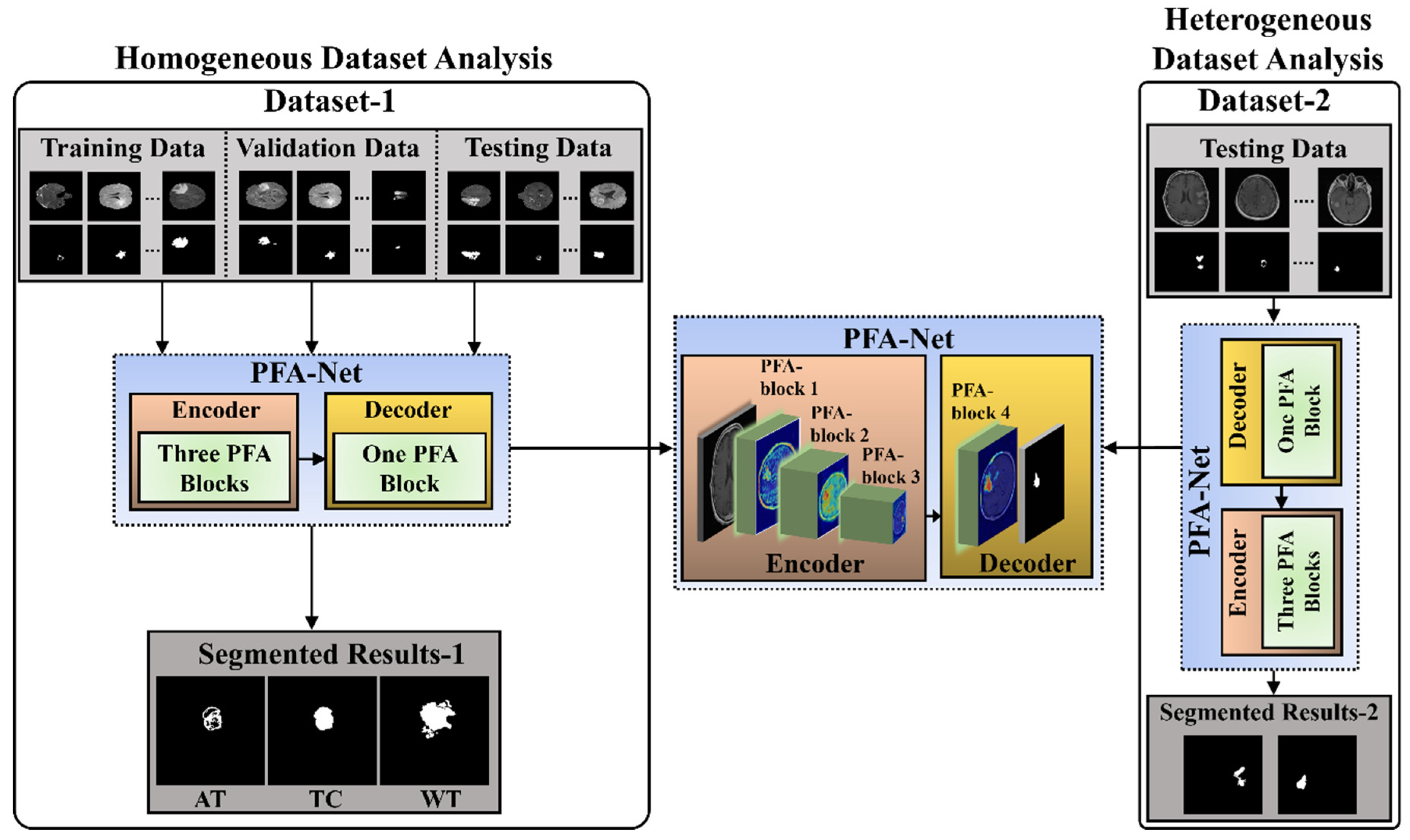
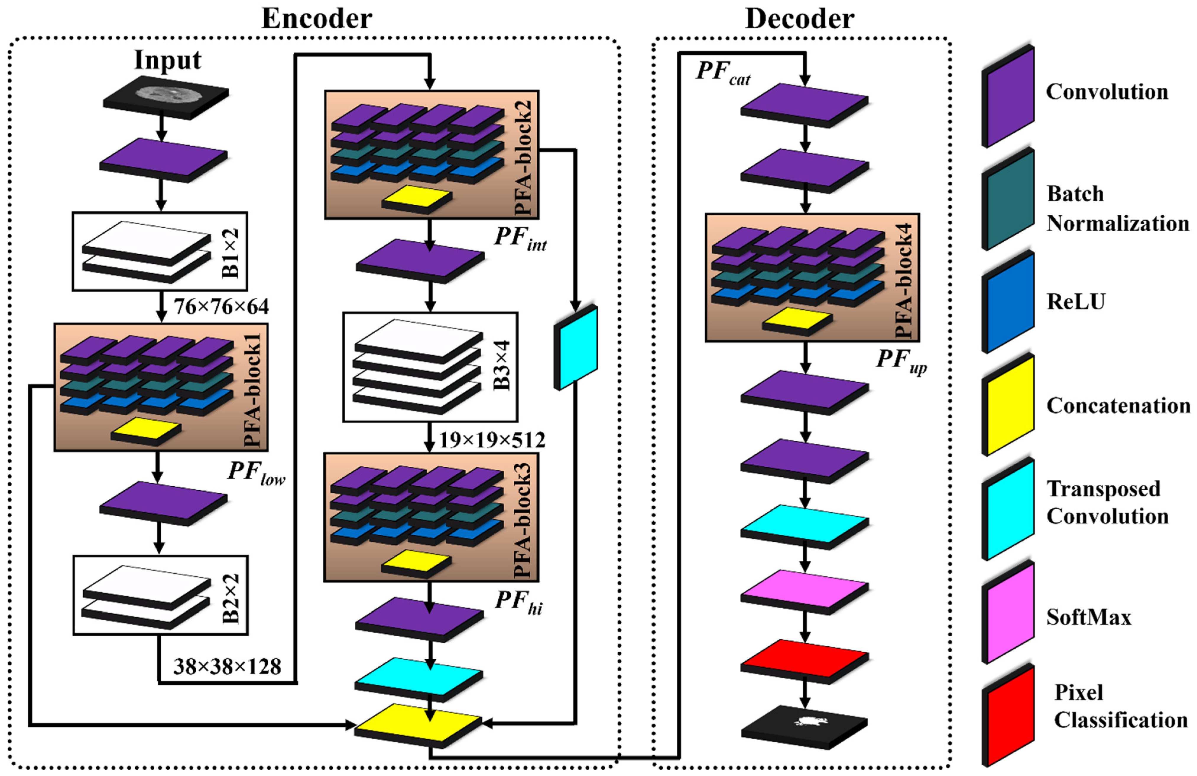
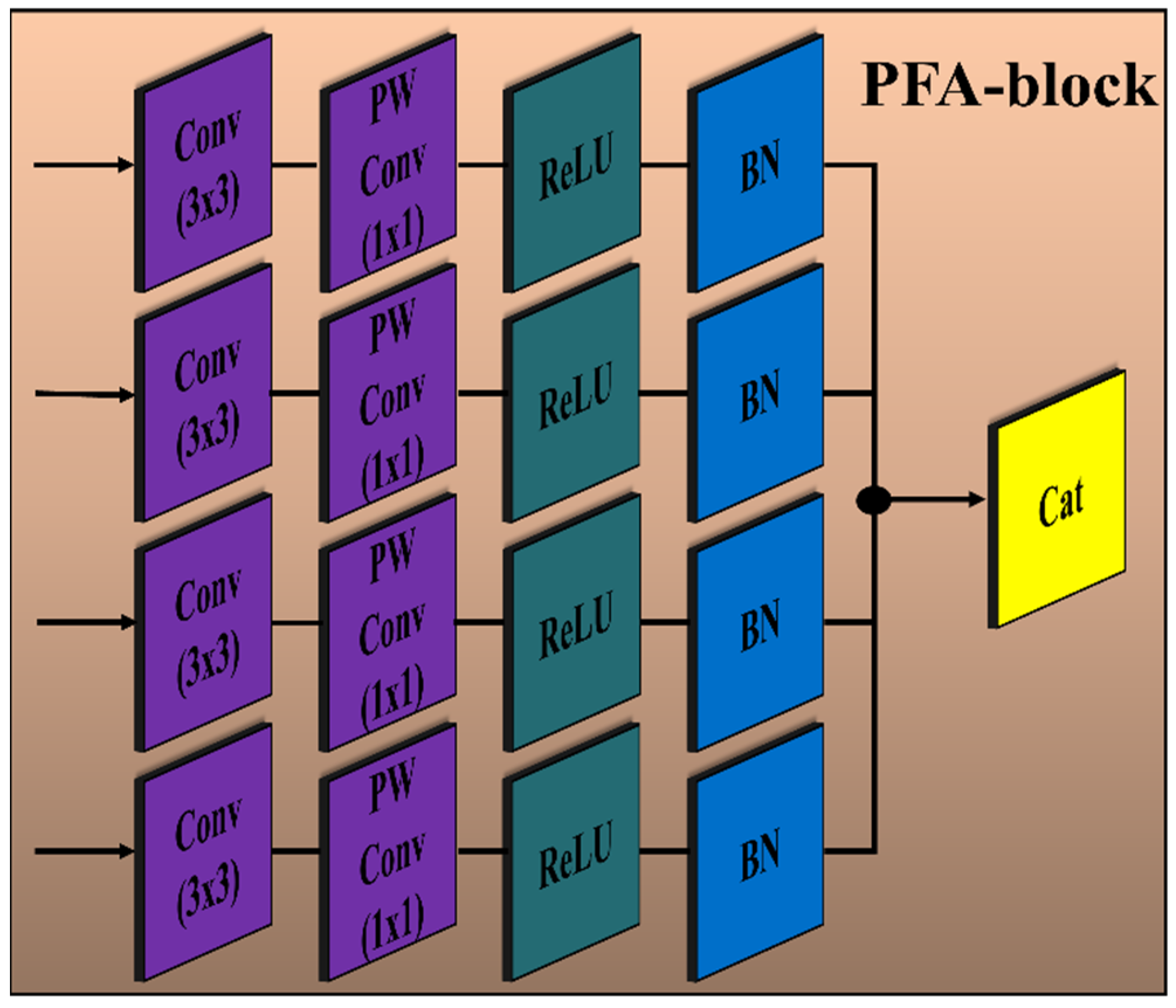

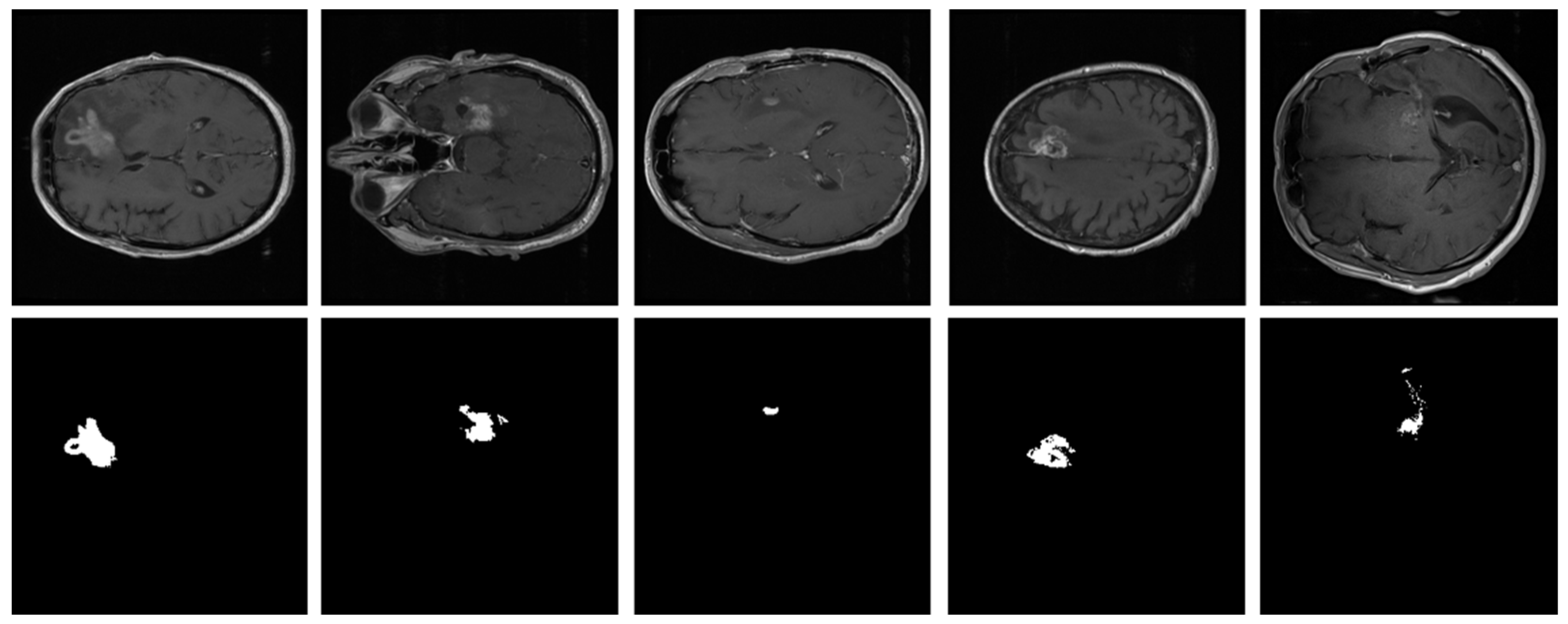
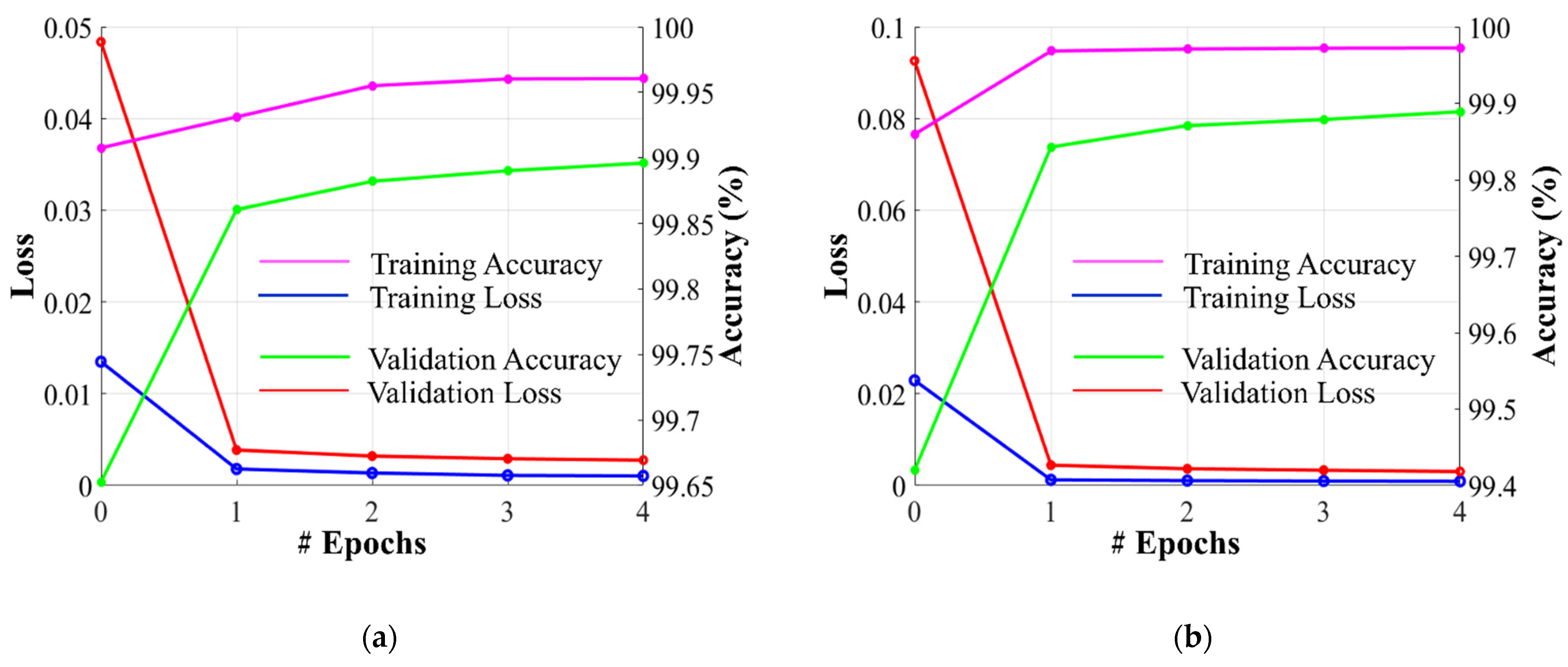
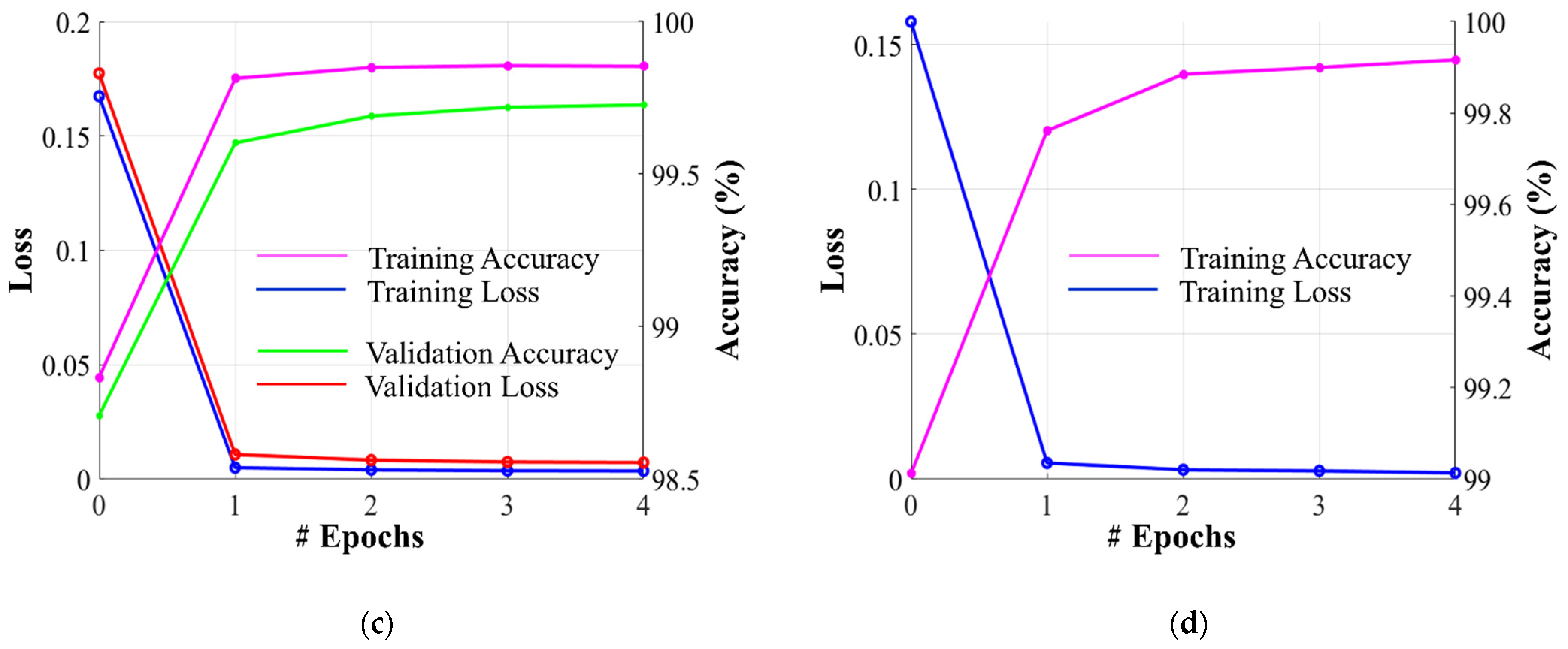

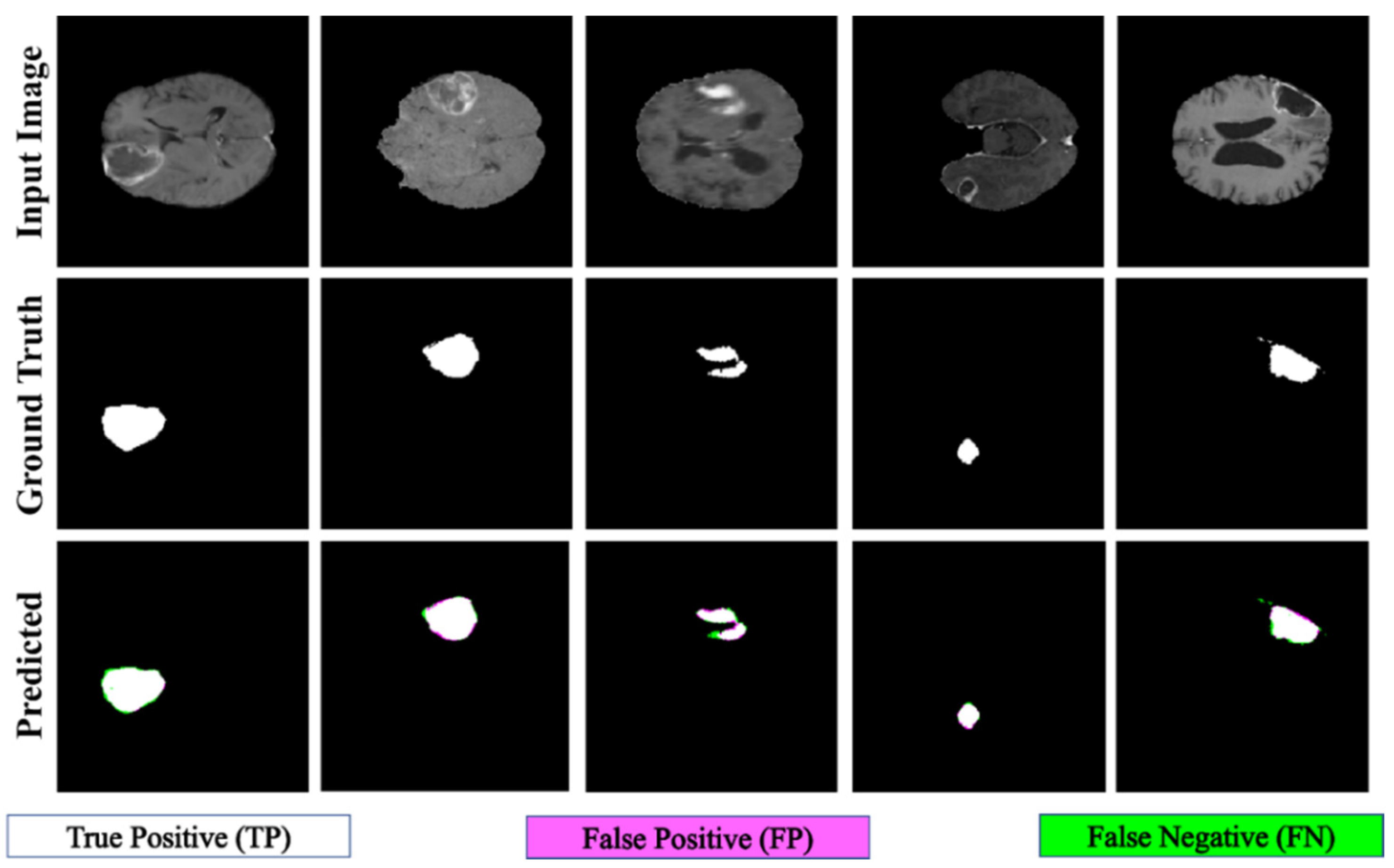

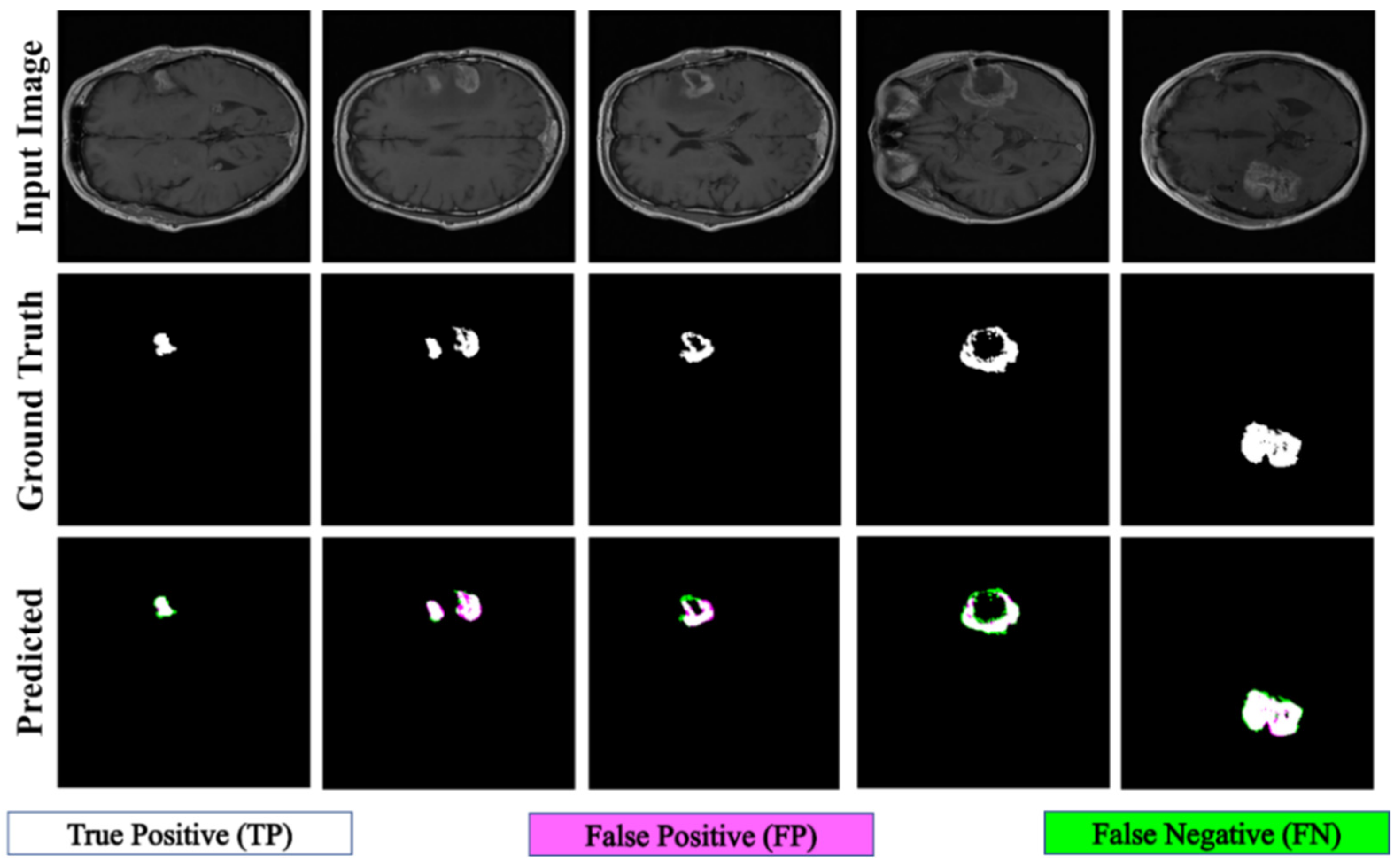
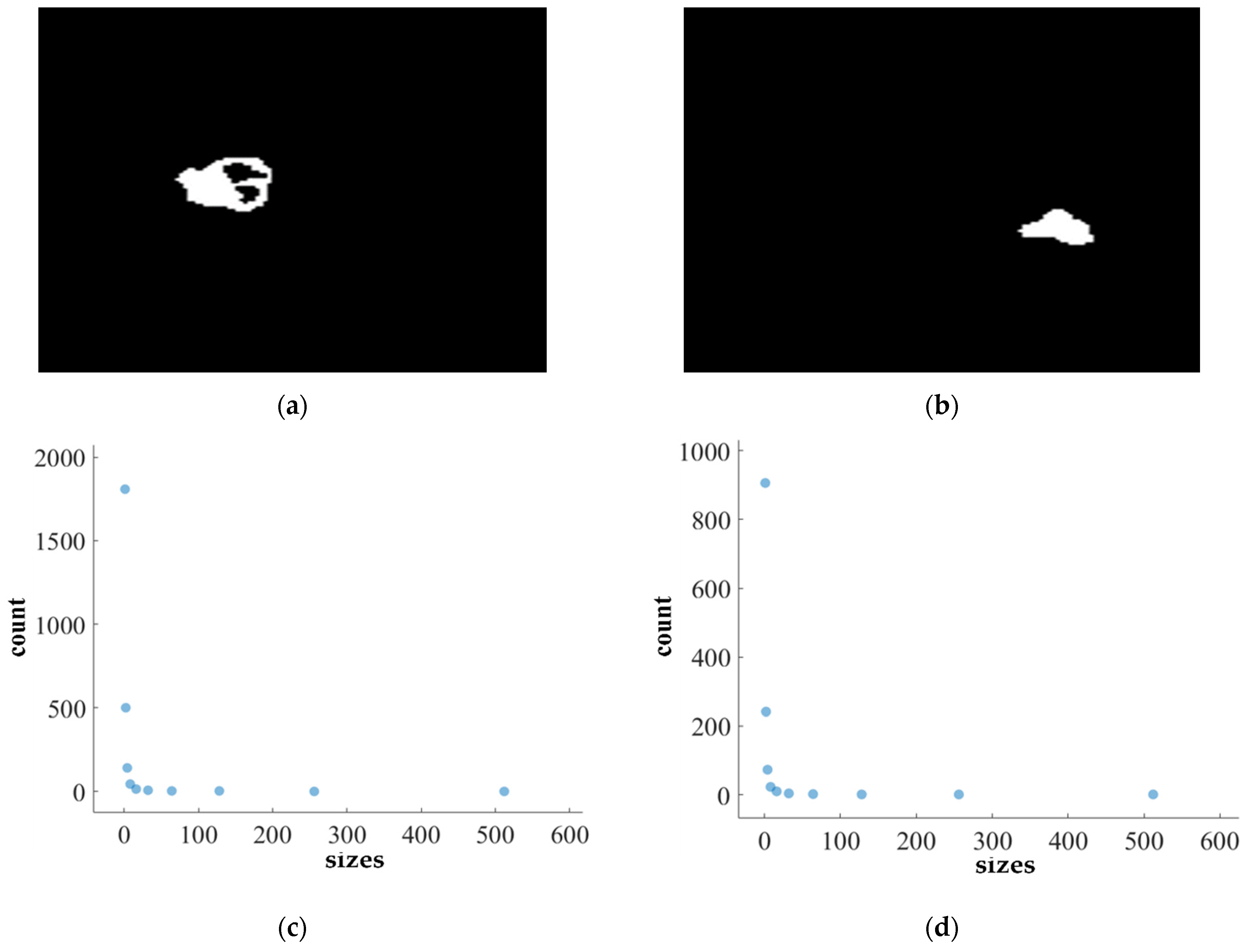
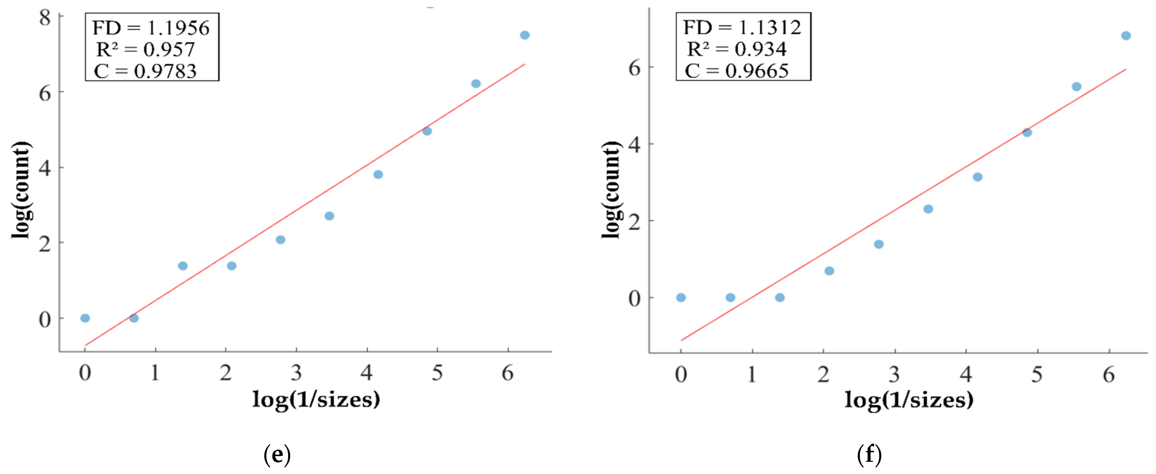
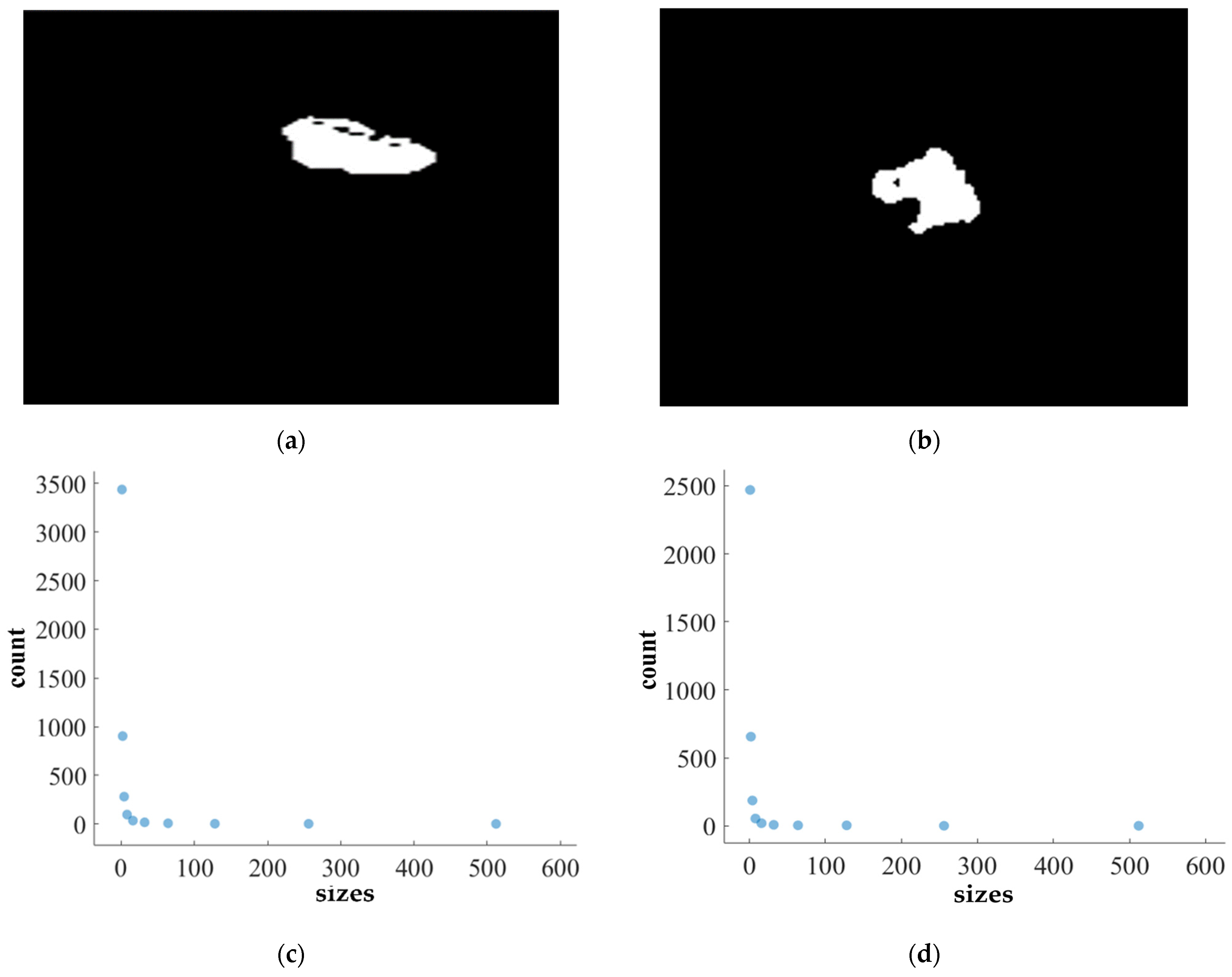
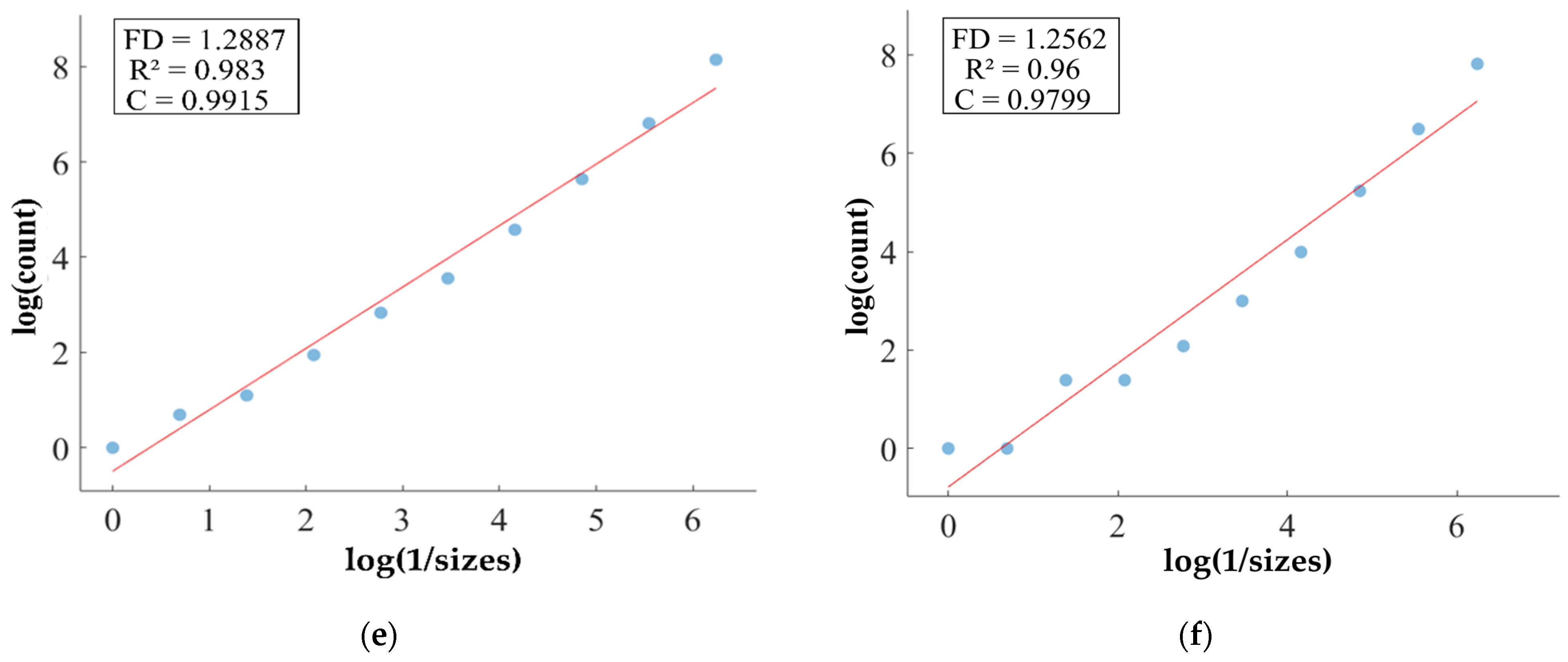
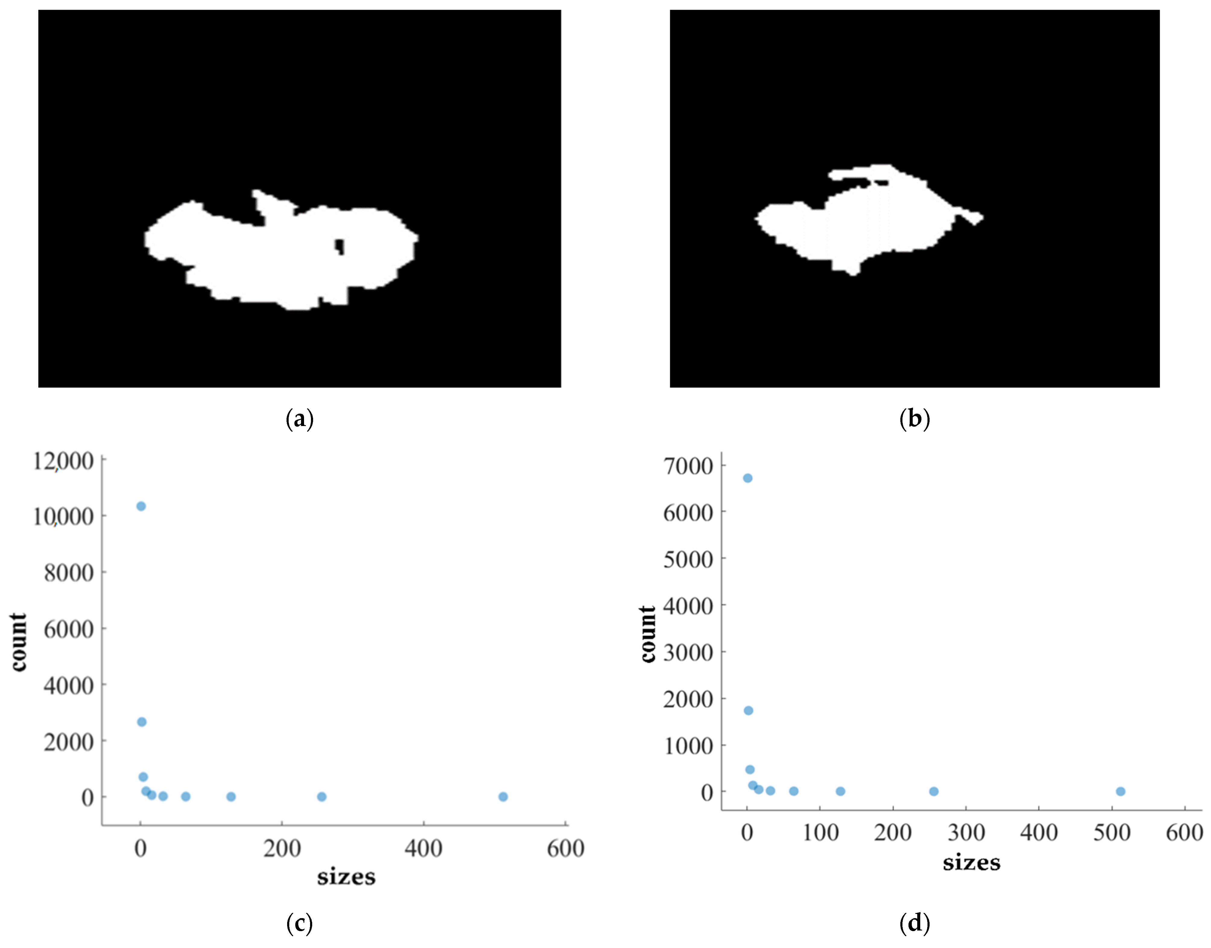
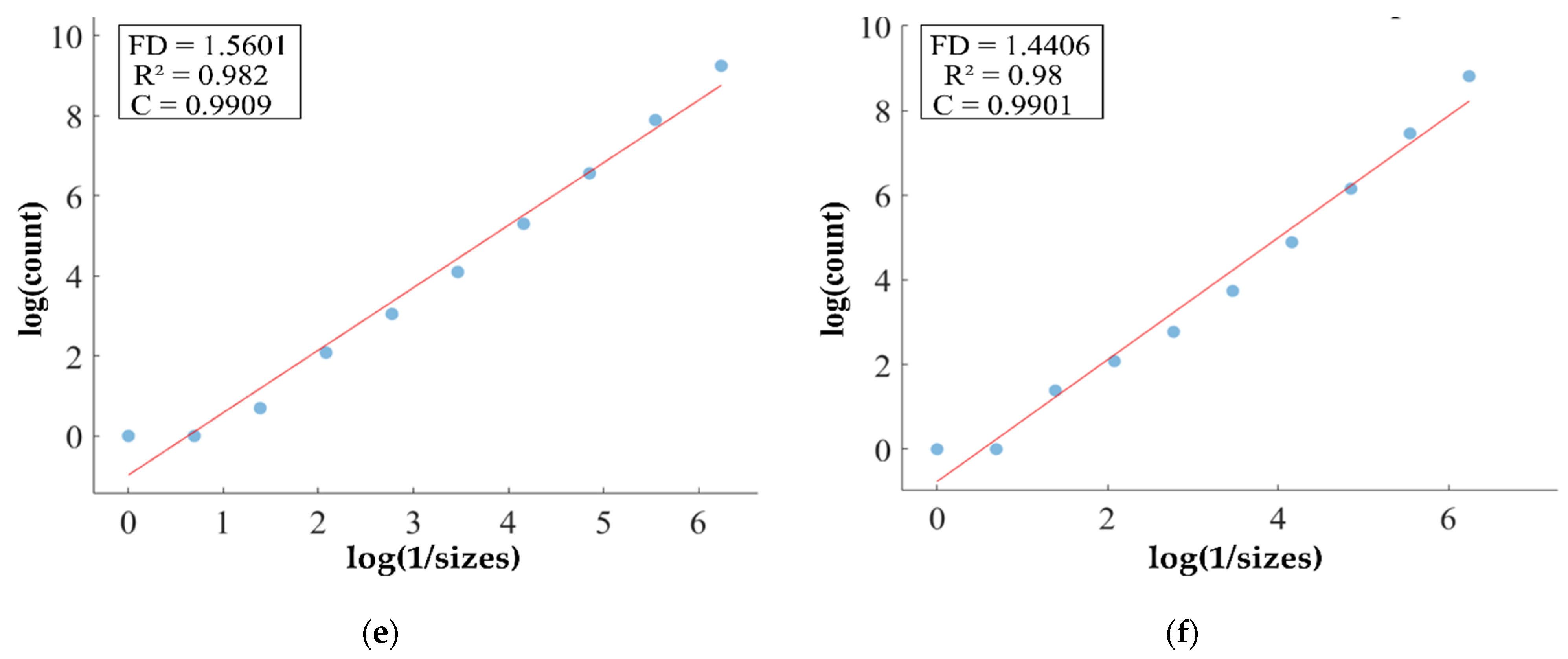
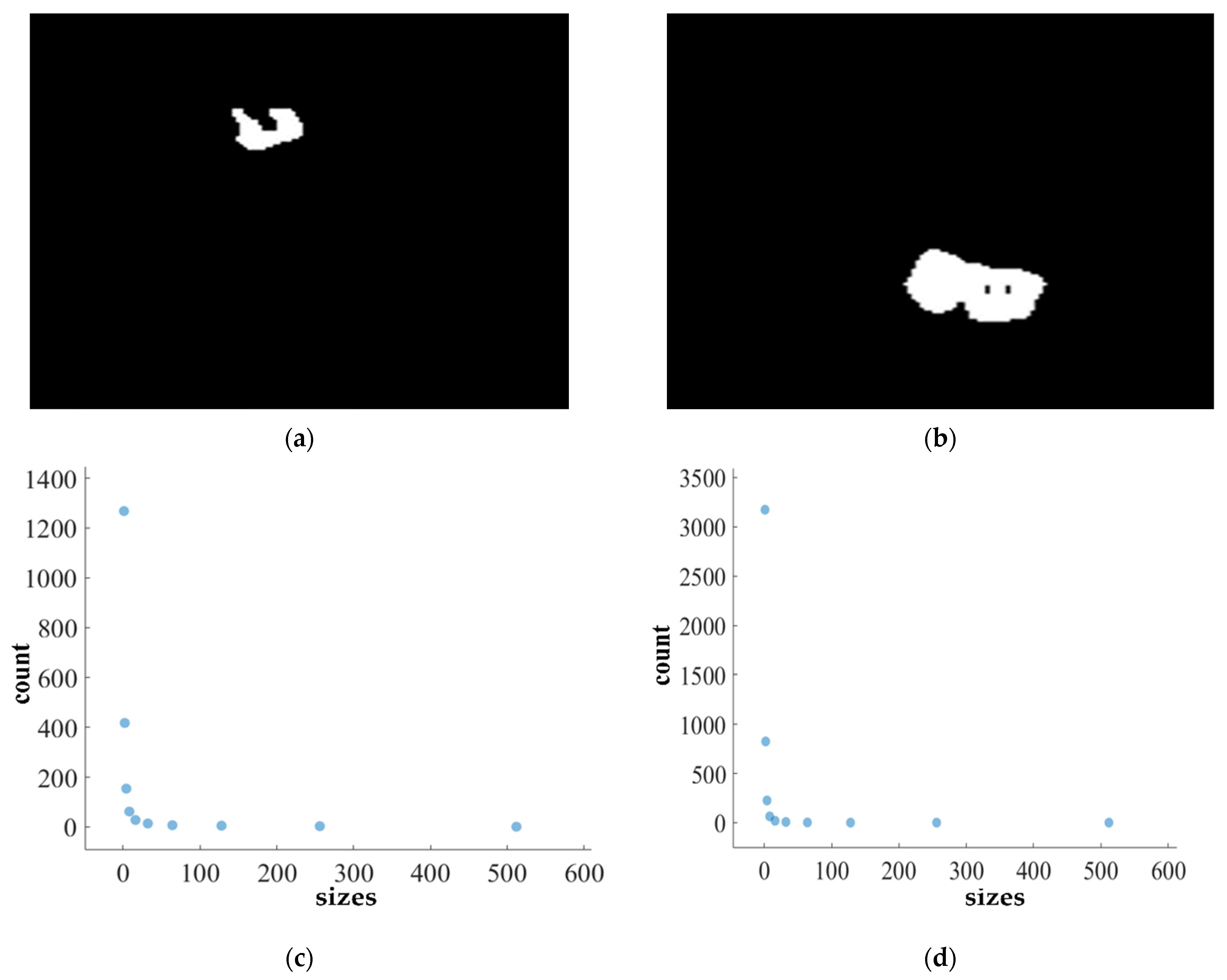
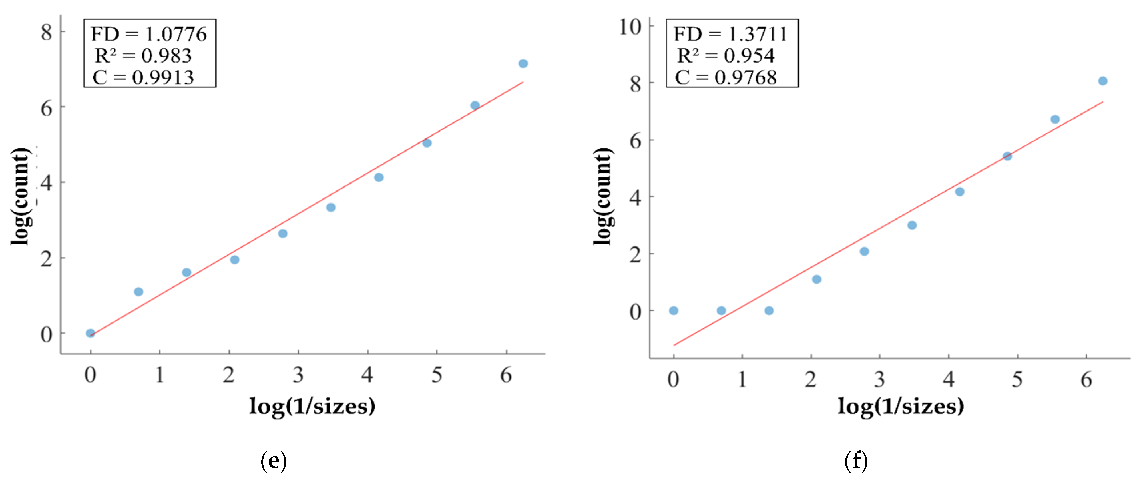


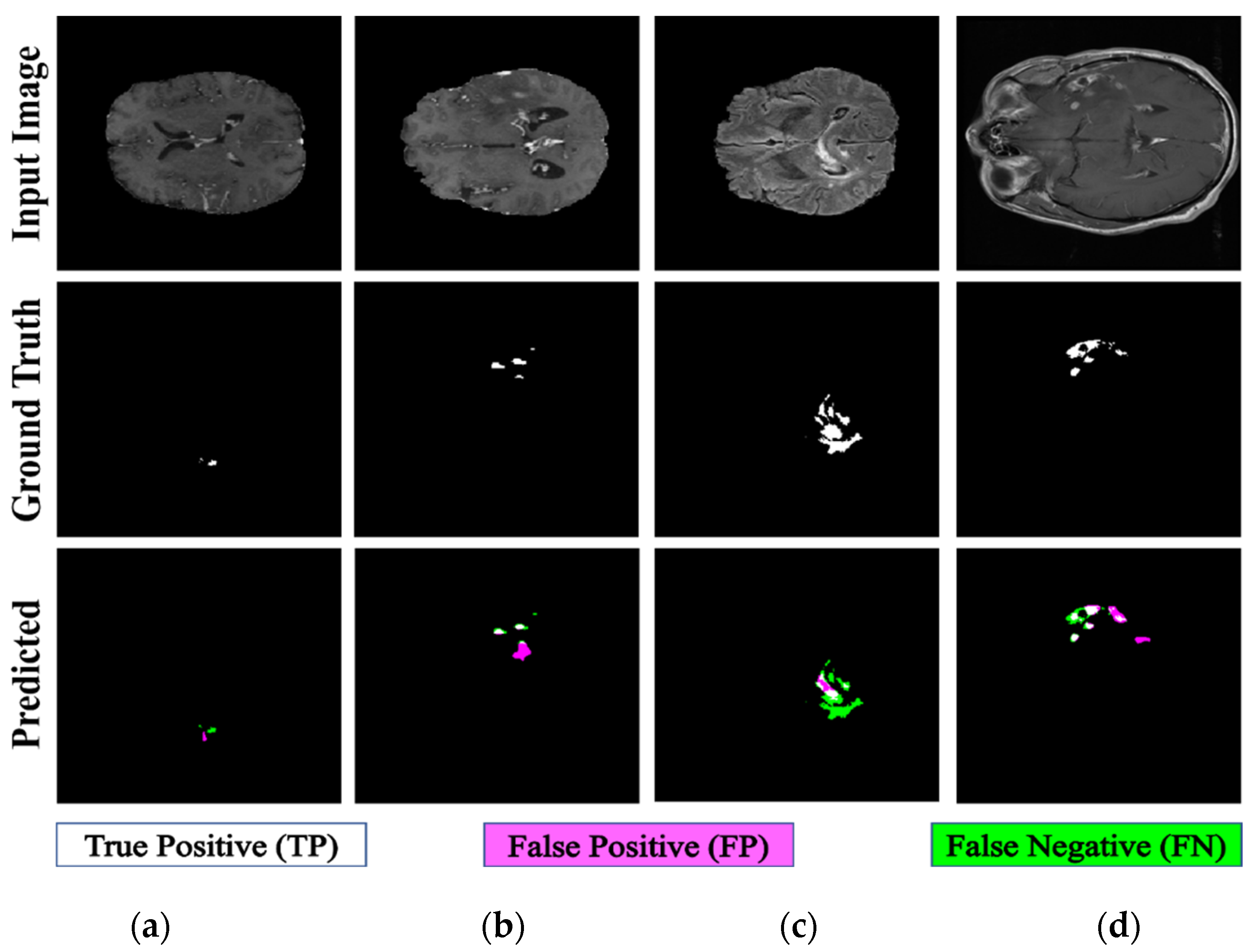
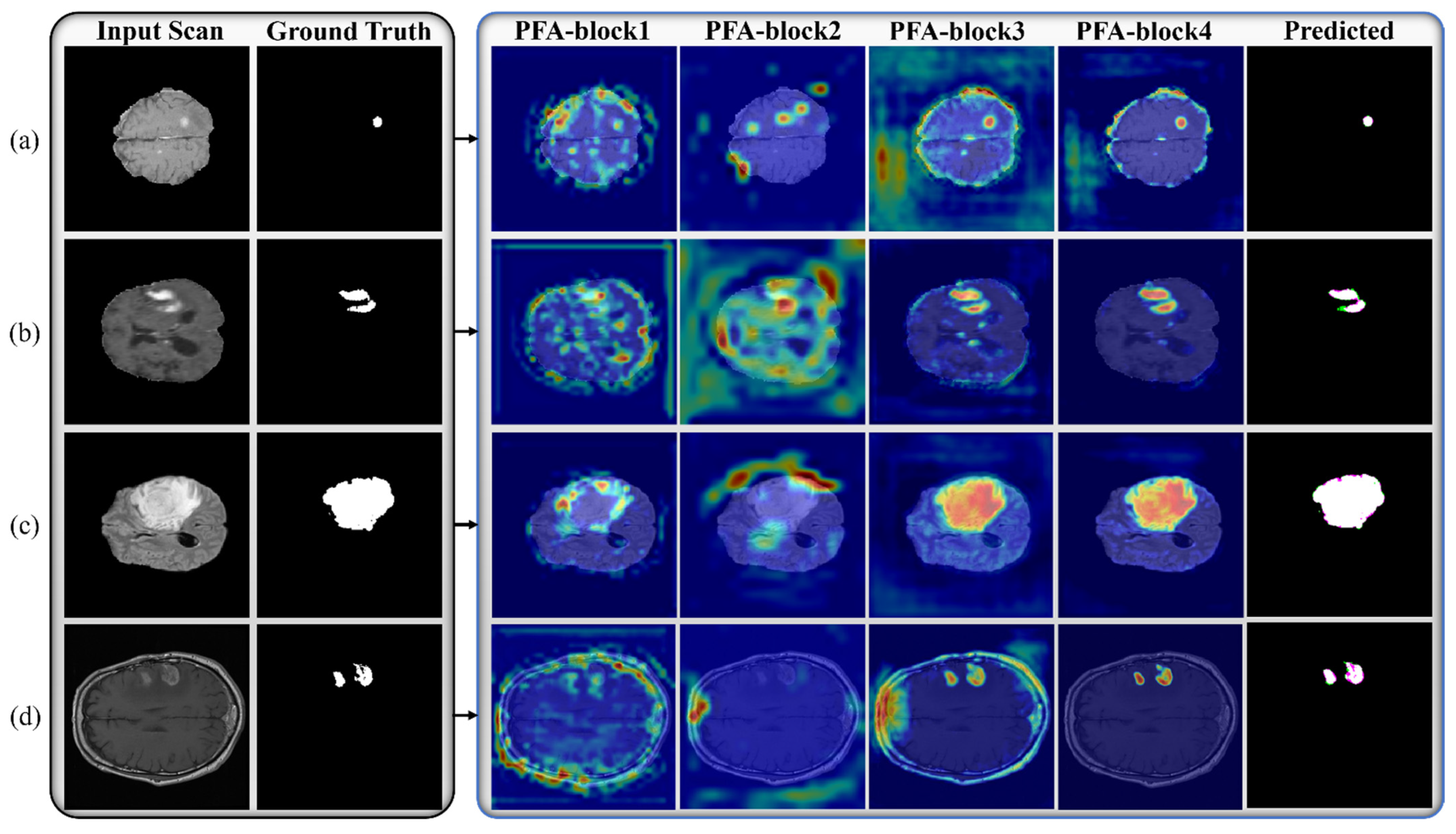
Disclaimer/Publisher’s Note: The statements, opinions and data contained in all publications are solely those of the individual author(s) and contributor(s) and not of MDPI and/or the editor(s). MDPI and/or the editor(s) disclaim responsibility for any injury to people or property resulting from any ideas, methods, instructions or products referred to in the content. |
© 2024 by the authors. Licensee MDPI, Basel, Switzerland. This article is an open access article distributed under the terms and conditions of the Creative Commons Attribution (CC BY) license (https://creativecommons.org/licenses/by/4.0/).