Abstract
This article introduces a novel optimization approach known as fractional order whale optimization algorithm (FWOA). The proposed optimizer incorporates the idea of fractional calculus (FC) into the mathematical structure of the conventional whale optimization algorithm (WOA). To validate the efficiency of the proposed FWOA, it is applied to address the challenges associated with the economic load dispatch (ELD) problem, which is a nonconvex, nonlinear, and non-smooth optimization problem. The objectives associated with ELD such as fuel cost and wind power generation cost minimization are achieved by taking into consideration different practical constraints like valve point loading effect (VPLE), transmission line losses, generator constraints, and stochastically variation of renewable energy sources (RES) integration. RES, particularly wind energy, has garnered more attention in recent times due to a range of environmental and economic factors. Stochastic wind (SW) power is also included in the ELD problem formulation. The incomplete gamma function (IGF) quantifies the influence of wind power. To assess its efficacy, the suggested approach is applied to a range of power systems including 3 generating units, 13 generating units and 40 generating units, consisting of 37 thermal units and 3 wind power units. To further strengthen the performance of the optimizer, the FWOA is hybridized with the interior point algorithm (IPA) to further refine the outcomes of the FWOA. The FWOA and IPA are used to address the problem of ELD while including the unpredictable nature of wind power. The simulation results of the suggested technique are compared with the most advanced heuristic optimization methods available, and it has been observed that the proposed optimizer obtained a superior and refined solution when compared to other state of the art optimization techniques. Furthermore, the efficacy of the suggested strategy in enhancing the solution of the ELD issue is validated through statistical analysis in terms of minimum fitness value.
1. Introduction
Over the past few decades, a consistent rise in the demand of electrical power energy has been observed. This can be attributed to various factors including urbanization, population growth, and the widespread use of electrical appliances in homes, offices, and the industrial sector. It has become more challenging to manage power systems reliably and efficiently due to increased energy demand and integration of stochastically varying renewable energy sources (RES) in the conventional power system. Significant generational, operational, and maintenance expenses will arise under these highly strained settings. In addition, there will be an escalation in power losses, stability issues, and power breakdown incidents. ELD is of significant relevance in today’s contemporary power system due to the rising cost of electrical energy generation and the decreasing quantity of fossil fuels that are utilized in thermal power generating units. The main goal of the ELD problem is to effectively allocate the real power generating production from thermal power production units, considering the practical constraints placed on the electric power grid. Optimizing the allocation of active power generation in the system reduces generating costs and enhances the dependability of the electrical energy generation, hence enhancing the total energy capabilities. The research community is increasingly interested in addressing the traditional ELD issue in a realistic manner, given the myriad actual circumstances related with power systems. The fuel cost generation curve for both input and output is characterized by its non-differentiability, convexity, and linearity. This is due to the existence of bilayer heat generating valves in contemporary steamed-operated thermal energy producing units, often known as VPLE. By intentionally manipulating these steam valves, variations in the fuel-cost characteristic curve may be achieved. This can be mathematically expressed by including an absolute sine term into the fundamental quadratic function of the ELD problem [1]. Additional restrictions include restrictions on the speed at which the unit may increase or decrease during operation, as well as areas where the unit is not allowed to operate due to physical limitations of machine components [2]. The ELD problem is defined as an optimization problem with stringent constraints, nonconvexity, nonlinearity, and nonsmoothness. The ELD problem is resolved by conventional methods like linear and non-linear programming [3,4]. The methodologies used include branch and bound [5] and the Lagrange relaxation method [6]. These approaches use heuristics to methodically organize the generating units in a sequential manner to ascertain the most efficient solution. These techniques are not optimal for resolving ELD issues on a large scale and with severe limitations, since they need the use of algorithms that take exponential time to perform. Effectively managing limitations is a vital component of techniques based on ELD. Penalty and feasibility approaches are two separate techniques used by optimization algorithms to handle the constraints they face [7]. When using the penalty technique, there is a risk of unintentionally violating both equality and inequality criteria during the search process. Typically, these situations often incur a substantial penalty, either fixed or variable, for each violation of the restrictions in the objective function [8]. Some penalty techniques, such as the stochastic ranking approach and the ∈-constrained approach, consider the violation of constraints as an independent objective function [9,10]. Nevertheless, these conventional methods are insufficient in properly addressing the ELD problems due to their intrinsic characteristics of being nonlinear, non-convex, and non-smooth. To overcome the constraints of conventional methods, several soft computing approaches have been reported in the existing literature.
The creation of energy from thermal power plants that use fossil fuels has resulted in an escalation in the emission of detrimental gases, such as nitrogen oxide (NOx), sulphur oxide (SO), and carbon monoxide (CO). To tackle these harmful concerns for the environment, computational approaches have been created to maximize the efficiency of power generation while minimizing the detrimental pollution [11]. The incorporation of RES, including wind and solar power, has substantially mitigated the issues associated with increased generation costs and noxious gas emissions. The integration of renewable energy sources (RES) into thermal energy facilities has led to modifications in the conventional quadratic equation used to calculate fuel costs. These improvements include the inclusion of Beta and Weibull distribution functions, which consider the random variations in the availability of both wind and solar energy, respectively [12,13].
Constrained optimization problems are unsolvable with conventional numerical techniques due to the rigid situations introduced by the incorporation of practical constraints into conventional ELD problems. These methods are frequently ensnared in local optimum regions and are incapable of producing global optimum results. To combat global optimum stagnation, numerous nature-inspired global optimum methods have been developed and devised throughout the years. The genetic algorithm (GA) is used in situations when numerical approaches are unable to provide globally optimal results [14]. Utilizing a modified form of ant colony optimization (ACO), [15] makes use of six unit-based hybrid energy generating units. In [16], it has been found that the evolutionary programming (EP) strategy is an effective countermeasure to nonlinear and rigid scenarios of ELD problems. A multiple-objective load dispatch problem with combined economic emissions is executed utilizing a differential evolution (DE) based approach [17]. In [18], an improved Tabu Search Algorithm (ITSA) has been used to solve ELD problem. Particle swarm optimization, also known as PSO, is a worldwide approach that is inspired by metaheuristic nature and is taken into consideration to obtain the best outcomes of ELD merged with stochastic wind (SW) constructing hybrid energy generation systems [19,20,21,22]. The optimization of wind power availability, along with thermal power production units, has been achieved via the use of a novel optimization method called HIC-SQP. The objective is to optimize the direct cost, exaggerated cost, and underestimated cost to minimize both the expense of power generation and the emission of dangerous gases. This approach has been recently developed and applied successfully [23].
A more recent recommendation suggests incorporating the concepts of fractional calculus (FC) and the fundamental principles of derivatives with fractions into the basic mathematics structure of a system, which might lead to significant improvements in several fields of science and engineering. Various issues, including feature selection, fractional order filters, Kalman filters, and robotic motion controllers have been successfully solved and handled by this concept. According to the results of this research, it is advised to combine FC techniques with metamorphic approaches to solve the constrained optimization problem in the power sector. A different version of fractional order robotic PSO was recalled, solving different engineering problems [24,25,26,27,28]. A multiband power system stabilizer is designed using a lead-lag compensator that incorporates a hybrid dynamic GA-PSO [29] and non-linear system identification [30]. Other applications include the use of fractional order moth flame in optimization engineering issues [31,32,33]. These investigations highly recommend combining FC approaches with metaheuristic algorithms to solve optimization difficulties in the power and energy sector.
The research indicates that many control parameters need to be adjusted for most algorithms. To get an ideal solution, it is essential to accurately calibrate the control parameters, a task that is both time-consuming and challenging. A novel method called fractional whale optimization algorithm (FWOA), which draws inspiration from fractional order calculus, has been introduced. This algorithm draws inspiration from the majestic creatures of the sea, whales, that are comparable to huge animals seen in nature. Whales can travel in a spiral motion due to the two-dimensional movement they exhibit in relation to bubbles. According to [34], this approach has shown swift rate of convergence and efficient exploitation abilities in resolving different engineering design problems by modifying just one control parameter. Nevertheless, in the conventional WOA, during its last stage of optimization, approximately all individuals in the population tend to converge towards a narrow area around the current optimum solution. In complex multimodal global optimization problems, the entire populace may rapidly merge to the local optimal point. A solution to this problem is provided, which involves using a modified version of the Whale Optimization Algorithm (WOA) known as the FWOA-IPA approach. This modified version integrates the idea of local quick local search strategies to enhance the exploration and exploitation capabilities of FWOA. The objective is to address the constrained optimization issue of ELD combined with chaos infused stochastic wind power. According to our literature review, the potential of FWOA based heuristics has not been used in ELD studies including integrated power resources. Thus, this study investigates the potential for optimizing algorithms in integrated load dispatch studies.
While renewable energy sources hold promises to address environmental concerns, effectively integrating varying supplies like wind power introduces tremendous complications for the electric grid. Traditional approaches struggle to handle the inherent unpredictability and nonlinear dynamics. Simple algorithms frequently terminate prematurely, neglecting better solutions, and fail to contingency plan for stochastic fluctuations in natural energy production. In contrast, novel techniques show potential to more skillfully manage such a vexing problem, carefully balancing the grid amid intermittent wind and remaining receptive to unforeseen changes. Though the challenge appears daunting, continued progress toward overcoming local optima and prolonging search lifetimes could help systematically tackle renewable energy’s integration complexities.
By introducing a degree of versatility and memory impact into the optimization process, FC proves to be quite beneficial. Using fractional derivatives, the algorithm can effectively adapt to dynamic changes and uncertainties in the problem, resulting in enhanced convergence attributes and solution accuracy. Including FC in WOA offers the following benefits:
- With the use of fractional derivatives, the search dynamics can be enhanced, providing a finer control over the search process. This improvement allows the algorithm to effectively avoid getting stuck in local optima and thoroughly explore the solution space.
- The inherent memory effect in FC enhances the ability to handle the unpredictable nature of wind behavior, resulting in a more resilient optimization process.
This paper’s main contribution is as follows:
- The primary contribution of this paper is to design a novel fractional memetic evolution algorithm that synergies the integration of fractional calculus with meta-heuristic computational paradigm of WOA algorithm for optimizing combined thermal and wind power plant system.
- This study includes wind power plants into the integrated power plants system to minimize the total generation cost. Additionally, the optimization of these rigid scenarios will be tested using the FWOA and its hybrid scheme.
- The stability, accuracy, and efficiency of the proposed optimizer is validated through statistical analysis.
- The proposed FWOA and FWOA-IPA are evaluated for their competence and efficacy with other state of the art optimization techniques in terms of minimum fuel generation cost.
The paper is organized in the following manner.
Section 2 of the study focuses on the mathematical modeling of the thermal generators’ ELD issue, considering physical constraints such as VPLE. Furthermore, a stochastic mathematical model has been constructed to address the issues of underestimation and overestimation that are often encountered in wind power forecast. The Section 3 and Section 4 provide the methodologies of FWOA and hybridized schemes, namely FWOA-IPA and ELD-SW, for solving ELD issues and ELD-SW, respectively. Section 5 encompasses the process of validating and verifying the projected outcomes of the hybridized computational heuristics of the FWOA algorithm. This is achieved via conducting comparison studies with existing approaches to demonstrate the efficacy of the proposed scheme.
2. System Model: Formulation of ELD Involving Stochastic Wind
The primary objective function, which demonstrates the correlation between active power output in megawatts (MW) and fuel producing cost in dollars per hour (USD/h), may be mathematically represented using a quadratic fuel cost function as described in Ref. [1].
FC1 represents the aggregate fuel cost in USD per hour of generation, while g denotes the entire count of thermal power generation units. Coefficients Z″, Y″, and X″ represent generation coefficients that account for social, economic, and other relevant factors for the given thermal power plant in the quadratic fuel cost function formulation.
To facilitate flexible power production, each individual thermal generating unit is equipped with a series of steam-operated valves that control the injection of steam into turbines, depending on the need for electrical power [1]. In traditional thermal power generating units, which consist of a steam generator (boiler), steam turbine, and alternator, the efficiency of the power generating unit increases significantly as the load demand increases. As the load demand increases, the generation cost rate in USD/h also increases. This behavior can be represented by a quadratic equation. However, load demand variations have also been addressed within contemporary thermal power generating units. Experts in the field regulate the electrical power generation via alternator by using controlled valves to manage the amount of steam sprayed on turbines through separate nozzle groups, in accordance with the load demand. Optimal efficiency is attained when each nozzle operates at maximum output. Optimal efficiency is achieved by opening the valves in a specific sequence to maximize output. During the valve point loading effect, the turbine operates at its peak efficiency until the next valve is opened in sequence. The outcome is an efficiency curve that exhibits ripples, achieved by incorporating a sine function into the primary quadratic equation used in traditional thermal power generation units.
The inclusion of absolute and sine components in the nonlinear quadratic function approximates this physical phenomenon, resulting in a non-smooth curve due to the ripples correspondent with VPLE.
Wm and Vm represent the generation coefficients associated with VPLE.
The integration of SW electrical power into thermal power producing units offers a notable benefit in terms of cost-effective and ecologically sustainable electricity generation. Power generating systems that combine thermal and wind power units have prompted the development of several models to characterize the timing of actual power output and operating expenses of generation. Various researchers have proposed different methods to calculate the total generation cost for systems that include both thermal and wind power generation. Wind speed varies unpredictably throughout the day, resulting in an uncertain power generation output from wind power generators. Operators in this regard may tend to overestimate or underestimate the availability of wind power generation. When wind power is overestimated, it means that the actual power available at the required time is lower than what the operator had predicted. The operator will procure power from alternative sources to meet the load demand. When it comes to the penalty for underestimation, if the wind power available exceeds the initial assumptions, it will go to waste. In such cases, it is only fair for the system operator to compensate the wind power producer for the loss of capacity. When we put the discussion in the format of an optimization problem, the mathematical model is based on the costs of overestimating and underestimating wind power generation, as well as the fuel costs of thermal power generation.
The following mathematical model may be used to describe the total cost of producing wind electricity [23].
where FC3 is the total cost of producing wind power and n is the total number of wind power generating units. The direct cost, overestimated cost, and underestimated cost associated with wind power producing units are referred to as FCWP (direct, i), FCWP (overestimated, i), and FCWP (underestimated, i), respectively. Wind power production output is directly associated with FCWP (direct, w) and may be quantitatively stated for the wth unit as follows:
According to Equation (4), the actual electrical output power for the ith wind power producing unit is denoted by WPi, and the direct electrical energy cost from that unit is represented by di, which is in USD/MWh.
FCWP (overestimated,i) refers to an imbalanced cost resulting from an overestimation for wind power availability. Because of a shortfall in electrical power from wind power generating units, this results in the acquisition of extra real power in megawatts, which may be expressed mathematically as:
Equation (6) gives the predicted amount of wind power overestimation, denoted as T (Uoe, i), for the ith wind power generating unit. The overestimation cost coefficient for the ith wind power generating unit is denoted by Srw, i and is expressed in USD per megawatt-hour.
Vin, Vout, and Vr stand for the wind speeds under cut-in, cut-out, and rated circumstances in meters per second, respectively. An intermediary component, Pr, is included in the formula V1 = Vin + (Vr − Vin) ∗ W/P1 ∗ Pr. Weibull distribution coefficients Si and Ei represent the size and shape factor of the ith wind power generating unit, respectively. WPi and WPr represent the produced and rated electrical power in megawatts for the ith wind power producing unit. Furthermore, the incomplete gamma function, which is defined by two parameters, may be stated mathematically as shown [25].
A conventional gamma function includes a single parameter.
FCWP (overestimated, i) is a penalty expense incurred due to underestimating the wind power availability when the actual active power from wind power units exceeds the expected active power. Compensation is offered to cover the costs of wind power suppliers.
When it comes to the ith wind power generating unit, the variable Cew, i stands for the cost coefficient for underestimate in USD per megawatt-hour. T(UE,i) is the expected value of the ith wind power producing unit’s underestimate of wind power.
2.1. Overall Objective Function
The total generating cost (TGC) in USD per hour may be represented by combining the quadratic fuel cost function (FC1) without V.P.L.E., the V.P.L.E. (FC2), and the available cost function (FC3) for wind power production.
2.2. Problem Constraints
2.2.1. Constraint of Power Balance
The primary constraint pertaining to power systems is the efficient generation of electrical power to meet the load demand of end users. The power balance equation makes sure that power generated must be equal to the power demanded plus additional transmission power line losses as shown in Equation (11). Each term is defined as follows.
Pm: Power generated by mth thermal power generator.
Pi: Power generated by ith wind power generator.
P. Di: Power demand of ith user.
P. Li: Transmission power line losses associated with ith transmission line
A mathematical expression reflecting transmission power line losses associated with transmission lines is presented in Equation (12).
The B-matrix loss formula, denoted as in Equation (12), represents the relationship between loss coefficients and the injected powers and . Each term in Equation (12) is defined as follows.
Pj: Active power injected at jth bus.
Bjk: Coefficients associated with the B-matrix that reflect power losses due to power flow between jth and kth bus.
Pk: Active power injected at kth bus.
Bjo: Coefficients related to power losses dependent to power injection at jth bus.
Boo: Constant term independent of power injection at any bus.
2.2.2. Capacity Checks of Generator’s Power
When modelling an ELD issue in the context of electric power production, it is crucial for units to function within the specified range of the lowest and highest production ability.
3. Design Methodology
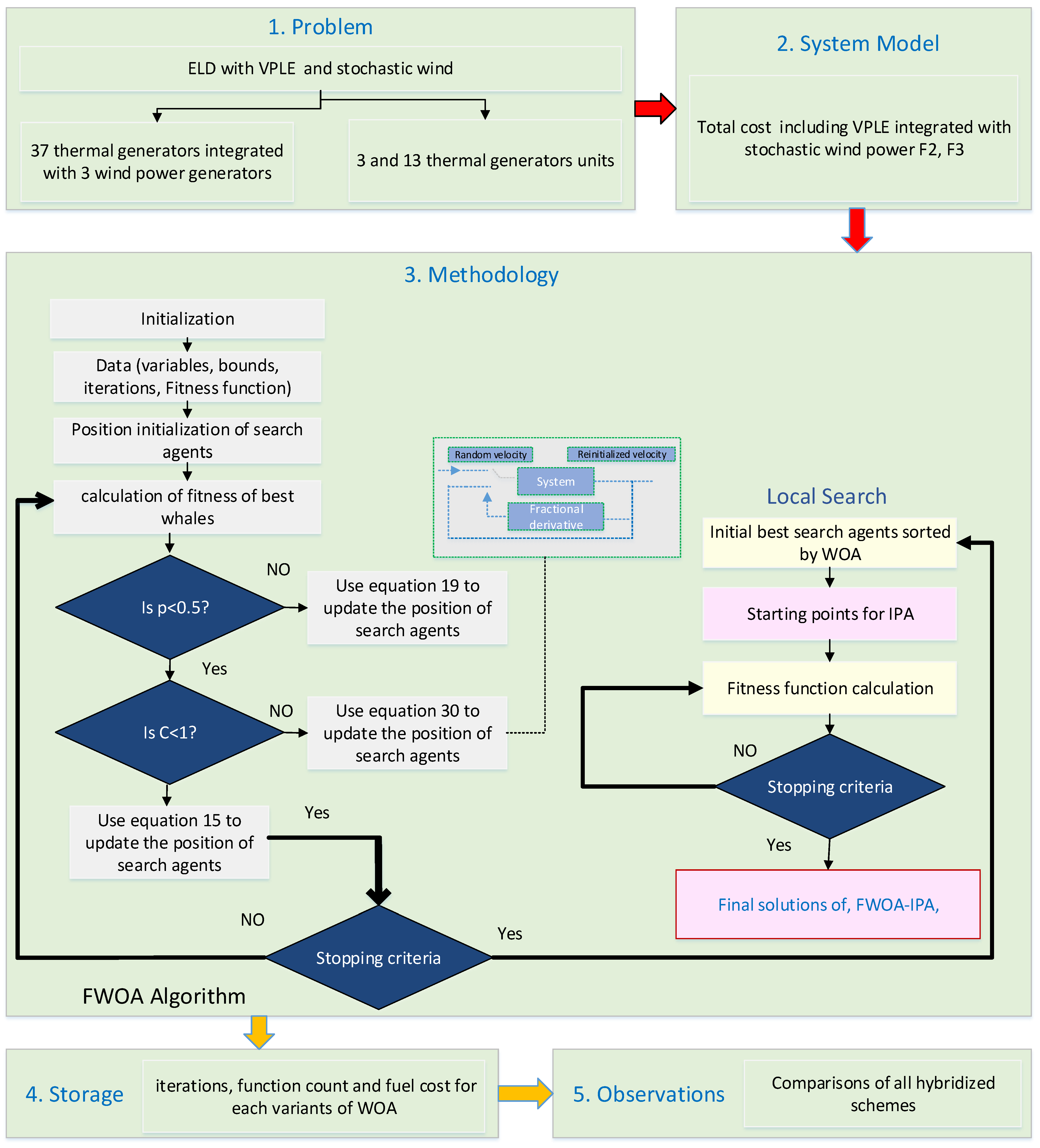
A hybrid approach is implemented to handle the constrained optimization problem of a power producing system. This approach combines a global search method based on the FWOA algorithm with a local search strategy called IPA. The goal is to obtain quick local convergence. To evaluate the effectiveness and efficiency of this hybridized scheme, three distinct case studies are investigated that include three, thirteen, and thirty-seven thermal generating units, as well as three wind power producing units. Figure 1 illustrates the methodology proposed.
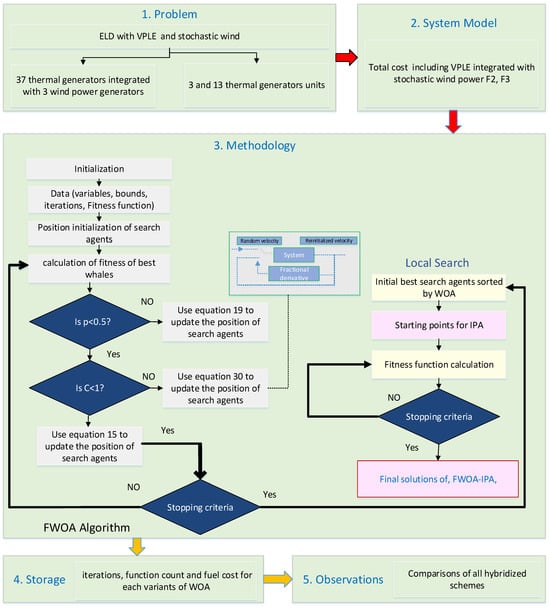
Figure 1.
Graphical overview of proposed methodology.
3.1. Whale Optimization Algorithm (WOA)
For the purpose of resolving optimization issues in engineering and mathematics, Mirjalili developed the WOA in 2016 [34]. This novel heuristic technique was inspired by nature and was designed to solve optimization problems. WOA is derived from the behaviors that are often seen in humpback whales. This optimization approach was modelled after the bubble net hunt strategy used by humpback whales. In this method, the whales move in a circular motion in order to capture small fish that are swimming near the surface. As a result of the fact that it is a behavior that is exclusive to humpback whales, this feeding technique is completely unique among nature-inspired optimization approaches. For the purpose of formulating the mathematical model of WOA, the bubble-net hunting operation is broken down into three distinct categories. After the first step of encircling the prey, the next stage is a feeding activity that involves a spiral bubble net, and the last stage is the search for prey. Every stage is described in this section.
3.1.1. Encircling Prey
The position of the object of attack and the prey is recognized by the humpback whales, and they proceed to encircle it. The greatest candidate advice is anticipated to be provided by the entity that is closest to the optimum plan. This is because the ideal approach for locating prey in the search location is not originally shared by all whales. The best searching agent is characterized, and consequently other search agents are updated to point in the correct direction of the top search agent. The following is one possible representation of this strategy:
where t represents the current iteration; represent the best solution in the position vector ; and and are the coefficient vectors. It is important to observe will be changed in each iteration, where represents the distance from the prey to the ith whale. Additionally, the vectors and are calculated according to Equations (17) and (18), respectively, in the following manner
where is a vector that has been generated at random and has a range that goes from zero to one and is reduced from two to zero for the phases of exploitation and exploration.
3.1.2. Bubble Net Attacking Method
Below, you can see two different techniques that humpback whales use to imitate this notion.
Shrinking Encircling Mechanism
This approach results from the estimation of a decrease from 2 to 0 as Equation (18) is repeated. In a similar vein, the altered scope of is diminished when the value of a, which is an arbitrarily selected value from [−a, a], is decreased. The initial position of search agents is determined by choosing random attributes for A within the interval [–1, 1], which falls between the primary location of each of the agents and the position occupied by the optimal agent.
Spiral Updating of Position
During this phase, the distance involving the whale (y, w) and the prey (y*, y*) is computed. A helix condition is subsequently established between the position of the whale and the location of the prey to replicate the spiral-shaped locomotion exhibited by humpback whales.
The symbol d denotes the distance or location between whale and its prey. Moreover, the constant b denotes the state of the logarithmic helix, while the arbitrary value falls within the range [−1, 1]. Since humpback whales execute a helix-formed course and swim in a contracting cycle around their prey, the likelihood of choosing either the helix strategy or the decreasing surrounding strategy is as follows:
3.1.3. Search for Prey
A comparable tactic, predicated on the variability of the vector , could be implemented during victim pursuit (exploration). An arbitrary examination of humpback whales demonstrates that they are discernible and visible to one another. It is also expected that a mobile search agent, situated at a distance from a reference whale, possesses proficiency in the behavior denoted by > 1. In addition, during the exploration phase, the update of a search agent’s position is determined by an arbitrary search agent, not the optimal pursuit agent that has been identified thus far. As such, the mathematical model is delineated:
3.1.4. Steps of WOA
The principal mechanisms of WOA are as follows: A predetermined set of randomly generated outcomes initiates the WOA. The coordinates of the pursuit agents are subsequently revised to reflect either the search agent’s arbitrary decision or the optimal outcome provided. In exploration and exploitation, the parameter “a” is reduced from two to zero. A randomized hunt agent is chosen when is greater than 1, and the optimal result for revising the positions of the pursuit agents is chosen when is less than 1. The change in motion from spiral to circular may be influenced by the value of p in this augmentation method. Finally, the WOA concludes upon fulfilment of the requirements. The entire WOA procedure is illustrated in Figure 1.
3.2. Interior Point Algorithm
The approach that appears to be most effective for addressing large-scale issues is to reduce the problem’s magnitude via nonlinear elimination [25]. The algorithm operates without the need for factorization of derivative matrices; thus, it is matrix-free. It employs iterative linear system solvers instead. Support for approximate step computations is implemented to reduce computational cost with each iteration. The algorithm in question is an extension of an imprecise Newton method utilized for equality constrained optimization, which incorporates supplementary capabilities to address inequality constraints. It is demonstrated that the algorithm converges globally under lax assumptions. Additional information regarding the IPA method is available in Ref. [35].
3.3. Fractional Order Whale Optimization Algorithm (FWOA)
FC has attracted the attention of a large number of academics as it may be used in a wide variety of scientific fields. These fields include engineering, computational mathematics, and physics, among others. Fractional calculus is a mathematical discipline that involves adjusting traditional calculus, which deals with integer-order derivatives and integrals. When it comes to expressing the memory and inherited attributes of processes, fractional derivatives are an appropriate tool to use since they are an inevitable extension of integer derivatives, also known as classical fundamental derivatives.
The concept of fractional order derivatives may be represented in several different ways, and there are multiple alternate techniques [36,37]. It is feasible to obtain the mathematical equations for FWOA that are based on the fractional order derivatives by using the Grunwald–Letnikov concept for fractional order derivatives. For any arbitrary information s(t) for which the Grünwald–Letnikov ordered fractional derivative is given in Equation (21), it is crucial to examine this signal [26].
While a derivative of numeral order only requires a finite sequence, a differential of fractional order requires an infinite number of elements. Consequently, “local” operators are those that are derived from integers. Fractional derivatives, on the other hand, must “remember” all the events that came before them. With the passage of time, however, the impact of previous occurrences becomes less significant. Equation (22) serves as the source of inspiration for the discrete time computation.
In this case, “r” stands for the data truncation order and “T” for the sampling time. When δ is equal to one, the equation becomes an integer order or normal first order derivative, and it may be expressed in the following way: ‘[s(t)]’ is discrete variable
The location for each whale is modified depending on its velocity, as indicated in Equation (24), to make use of the definition of FC that was presented before to improve the capabilities of the traditional WOA local search.
PSO motion is demonstrated by whales, with the local optimal flight path (LB. Fpos) reflecting the whales’ associated prey and the global optimal flight path (GB. Fpos) representing the best possible prey. At the end of each iteration, the location of every whale is updated based on the whale’s present velocity and position. Whales’ cognitive and social behavioral tendencies, as well as their original velocity, are compatible with the updated velocity according to the revised velocity. The distance between the local prey and their present position is the focus of the mathematical model of cognitive behavior as displayed in Equation (25).
According to Equation (25), the variables that are being considered are the velocity that corresponds to the nth whale at iteration t, the velocity at iteration t − 1, the local optimum location at t − 1, and the global best position at t − 1. Constant parameters C1 and C2 are used to reflect the intellectual and societal behaviors of whales for the local and global ideal positions, respectively. These parameters are referred to as C1 and C2. The random numbers r1 and r2 are utilized to determine the ideal arrangement of whales. These integers range from 0 to 1, and they are calculated at random. Equation (25) may be expressed using the formula expressed in Equation (26).
In the case when a fractional order differential is assumed to be equal to one, Equation (26) shows an integer’s first order difference. This makes it a classic example of the integer order derivative. Putting T equal to one and applying Equation (26) results in the following equation.
According to the FC concept, the order of velocity derivatives may in fact be generalized with a real number that falls between 0 and 1. This will result in a fluctuation that is smoother and a memory effect that lasts for a longer period. The Equation (27) may be redefined as follows, taking into consideration the discrete-time fractional differential:
The following equation describes the fraction acceleration for the nth searching agent: From 1 to 3.
Equation (29) may be restated in the following manner by taking into consideration only four terms:
3.4. The FWOA-IPA Method for Solving ELD Problem
The FWOA-IPA method can be employed to resolve the optimization problem outlined in Section 2. The FWOA-IPA method applies the main approach FWOA to the optimization problem and utilizes the optimal solution acquired through FWOA as the starting point for the IPA technique. In this regard, the letter “w” is regarded as the initial whale. One vector containing Nvar elements constitutes each cetacean. Nvar is a case-specific parameter that corresponds to the quantity of power facilities. Consequently, the proposed technique for resolving the ELD problem aims to ascertain the active power of the power plants in a manner that satisfies the constraints and minimizes the objective function. The FWOA-IPA method is believed to resolve the ELD problem through the following steps. The Pseudocode of FWOA-IPA is given in Algorithm 1.
Step 1: Initialize population size (NP), number of design variables and meeting criteria, number of objective function evaluations.
Step 2: Involves the computation of the objective function and the retention of the optimal solution.
Step 3: In Step 3, the parameters A, a, C, and l are updated randomly using fractional calculus parameters
Step 4: In the fourth step, a random number p is generated within the range of [0, 1]. If and C2 ≥ 1, mutate according to Equation (15); otherwise, update according to Equation (19).
Step 5: If the stop requirements are met, halt; otherwise, go to step 2.
Step 6: Save the best whale as best solution and initial point for IPA method.
Step 7: Run the IPA.
| Algorithm 1: Pseudocode of FWOA-IPA |
| Set all parameters Evaluate each search agent based on their objective function value. X* = The best search agent Start optimization while (t < max iteration) For each distinct search generate random coefficient the C1 and C2 using fractional calculus with parameters if (p < 0.5) if ( < 1) Use Equation (15) to update the current search agent’s location. Else if () Select random search Xrand Use Equation (19) to update the current search agent’s location End if Else if (p ≥ 0.5) Use Equation (30) to update the current search agent’s location end if end for check if any search agents out of search space objective function evlautions of each search agent update X* if there is a best solution save the best solution and intial point for IPA t = t + 1 end while Return X* |
4. Case Study and Simulation Results
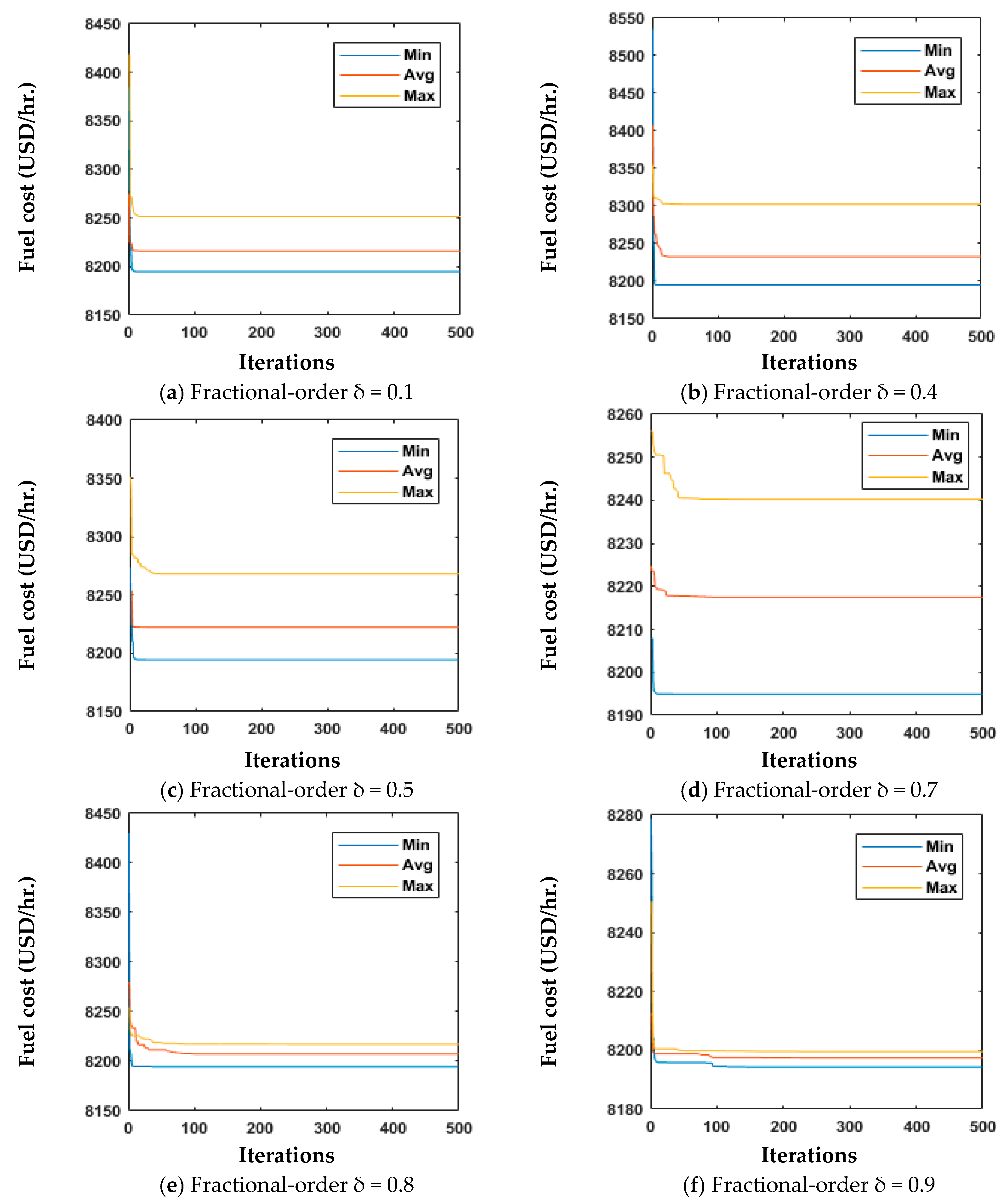
The proposed FWOA for reducing fuel generation cost via optimal allocation of power generation is assessed for its efficacy and application using three test systems. These systems consist of 3 generating units, 13 generating units, and a realistic Taiwan system with 40 generating units. Optimizing cost efficiency in power generating is a key priority for the intended purpose. The numerical values of the major regulating parameters are used as the basis for assessing the success of the suggested approach in electrical power system. Even a little change in the amounts of these components may lead to early saturation, resulting in a premature convergence and result. The FWOA parameters, which include the following: the size of the group, the number of whales, societal acceleration vectors, intellectual acceleration vectors, maximum iterations, fractional order of the velocity of whales, and separate runs are determined by testing and thorough analysis of an optimization issue. Table 1 displays the fundamental factors that must be modified to enhance the overall efficiency of the suggested algorithms. To enhance the effectiveness of the proposed method, the algorithms are executed with different proportions of fractional orders, which are determined based on the situation under examination. Evaluations are being conducted on 10 fractal order numbers, which range from 0.1 to 0.9. To determine the ideal scale for fractions evolving or swarming processes, an unpredictable technique is often used. The best sequence to follow is identified using Monte Carlo statistics, but selecting a fractional order with a strong physical justification is usually challenging. A statistical study of 20 trials is performed on all test cases to determine the strength and effectiveness of the FWOA optimization. The FWOA algorithm’s optimized findings have been combined with the IPA’s local search-based method for quick local convergence.

Table 1.
Initial settings of parameters for proposed FWOA.
4.1. Case Study 1: Three Thermal Generating Units Test System
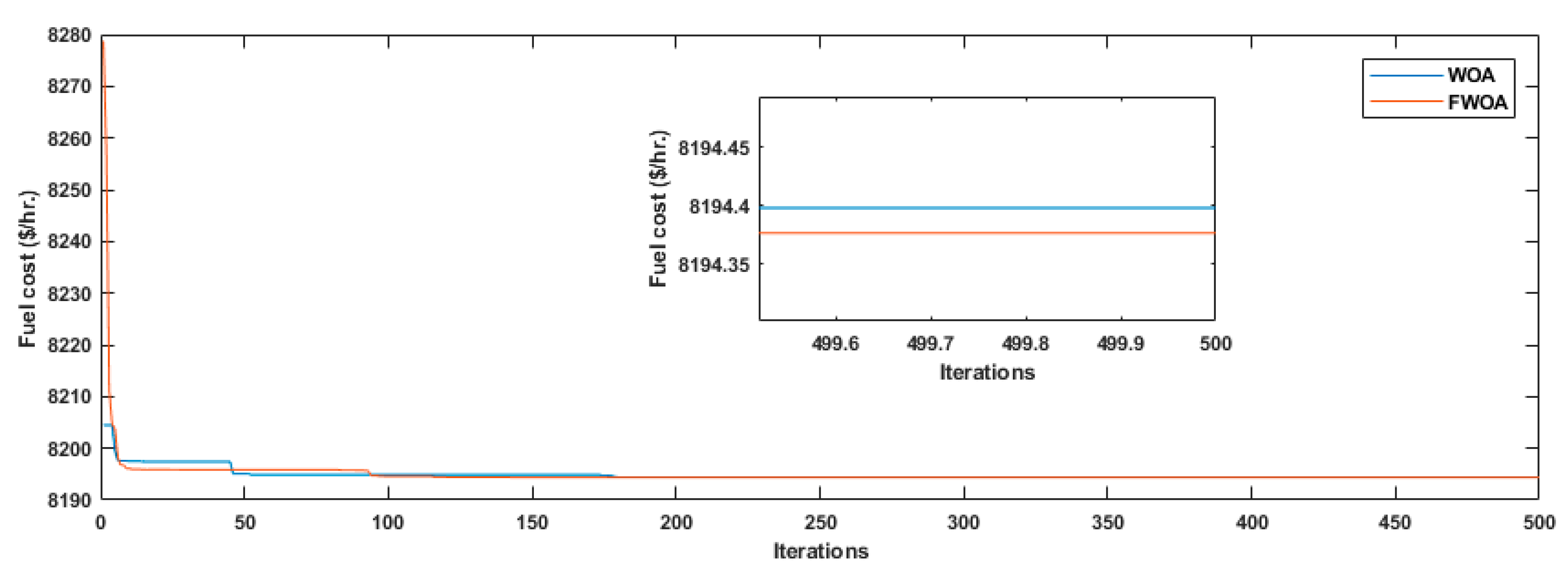
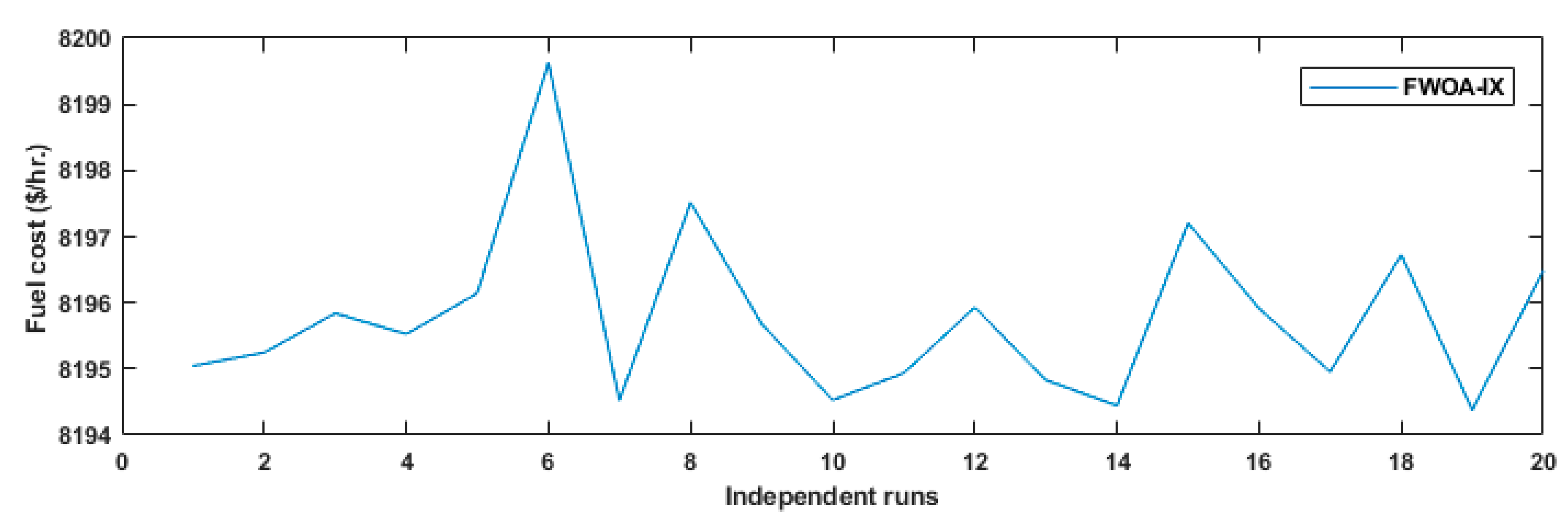
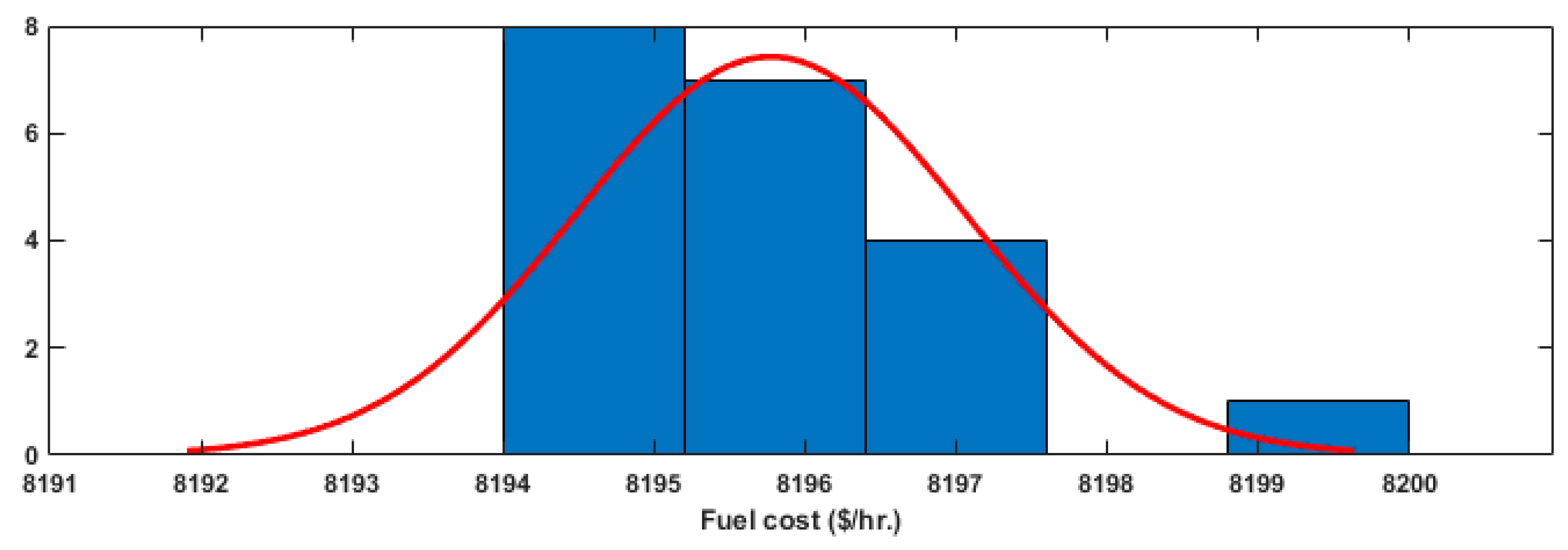
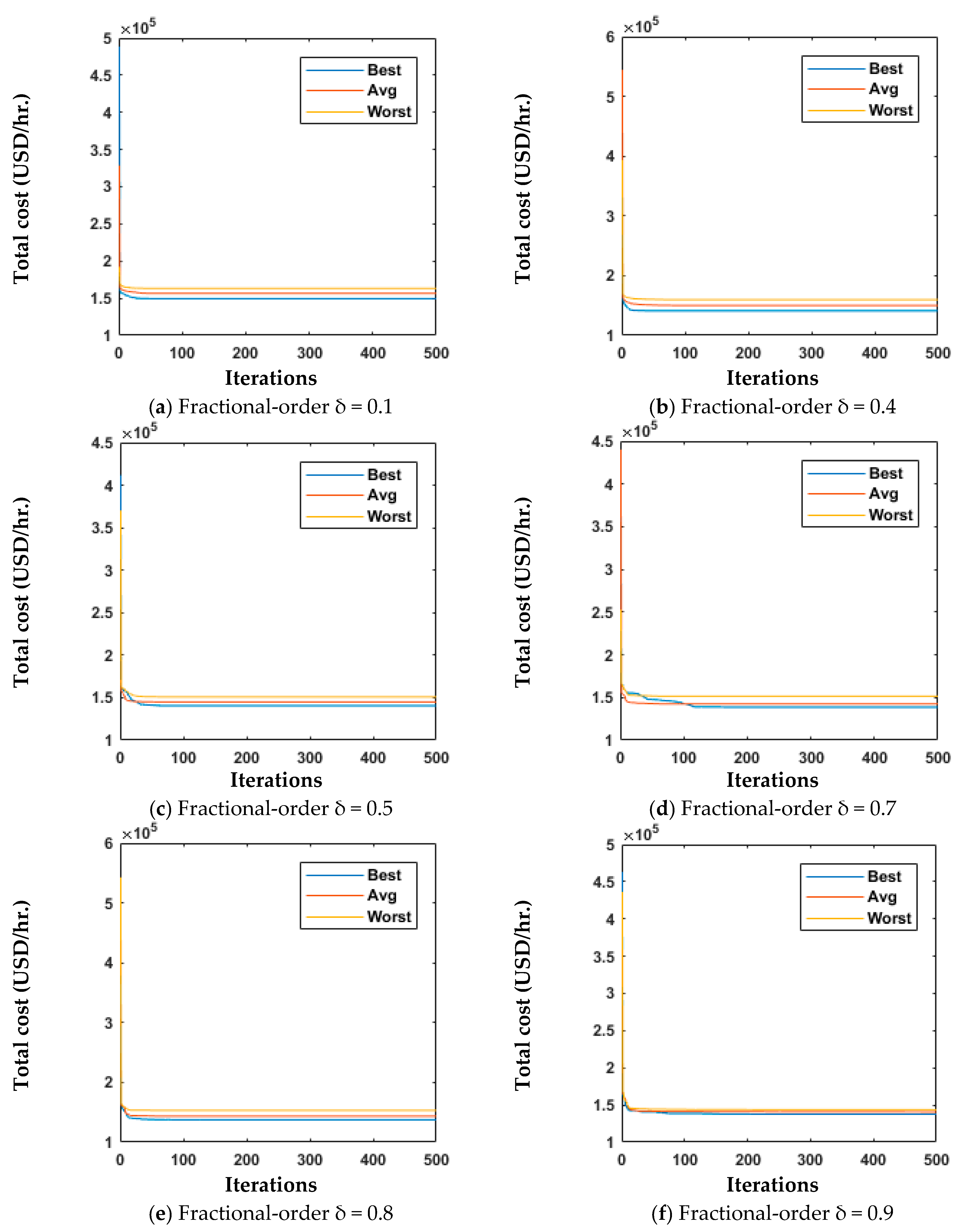
Case study 1 comprises of three thermal power-generators. The fuel cost coefficients for thermal power generators have been obtained from the Ref. [1]. During case study 1 power demand under consideration is 850 MW. Ten variations of the FWOA methodology are utilized in the examination of case study 1. The variants comprised an assortment of fractional order values, which varied in number from 0.1 to 0.9. It is impossible to ignore the stochastic unpredictability of the optimum outcome produced by the FWOA algorithm. To carefully observe the degree of deviations in optimum results, 500 iterations were utilized to execute 20 independent trials for every fractional order of the FWOA algorithm. Table 2 shows the outcomes of the simulation of the cost of fuel value (in USD per hour) associated with every fractional order of the FWOA algorithm across 20 different trials as well as the values used to extract variables related to the active power production output in megawatts for the FWOA variations. Figure 2 shows convergence characteristic curves over a range of different fractional orders. Table 3 presents statistical findings about the average and variation of fuel output rates. Out of the ten fractional orders of the FWOA algorithm, FWOA-IX with fractional order δ = 0.9 demonstrates the most advantageous simulation results regarding the minimum fuel generation cost of 8194.3762 USD per hour. The efficacy of the technique is illustrated in Figure 3, which encompasses convergence characteristics curve of FWOA-IX and conventional WOA algorithm. Figure 4 and Figure 5 display the 20 independent trials and histogram pertaining to the optimal variant of FWOA, specifically FWOA-IX.
Table 2.
Comparative assessment of the proposed FWOA algorithm for a Case study 1.
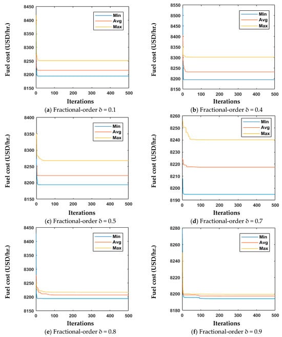
Figure 2.
Convergence characteristic curves of proposed FWOA algorithm in case of three thermal generating units test system.
Table 3.
Statistical findings for fuel generating cost in term of means and standard deviations for case study 1.
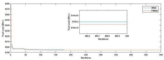
Figure 3.
Fitness curve of best variant FWOA-IX and conventional WOA for case study 1.
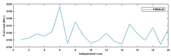
Figure 4.
Independent runs observations of variant FWOA-IX for case study 1.

Figure 5.
Histogram observations of variant FWOA-IX for case study 1.
Table 4 provides a summary of the minimum fuel costs specified by FWOA and their most recent equivalents from the literature, such as GWO, NSS, GA, EP, GSA, GAB, PSO, and PSO TVAC [38,39,40,41,42]. The percentage reduction in fuel cost includes 0.23% for NSS, 0.23% for GA, 0.22% for EP, 0.23% for GSA, 0.23% for GAB, 0.23% for PSO, and 0.71% for the proposed FWOA as shown in Figure 6.
Table 4.
Comparison of proposed FWOA algorithm with different solvers from literature for case study 1.
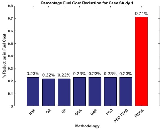
Figure 6.
Comparison of percentage fuel cost reduction for 3 generating units test system.
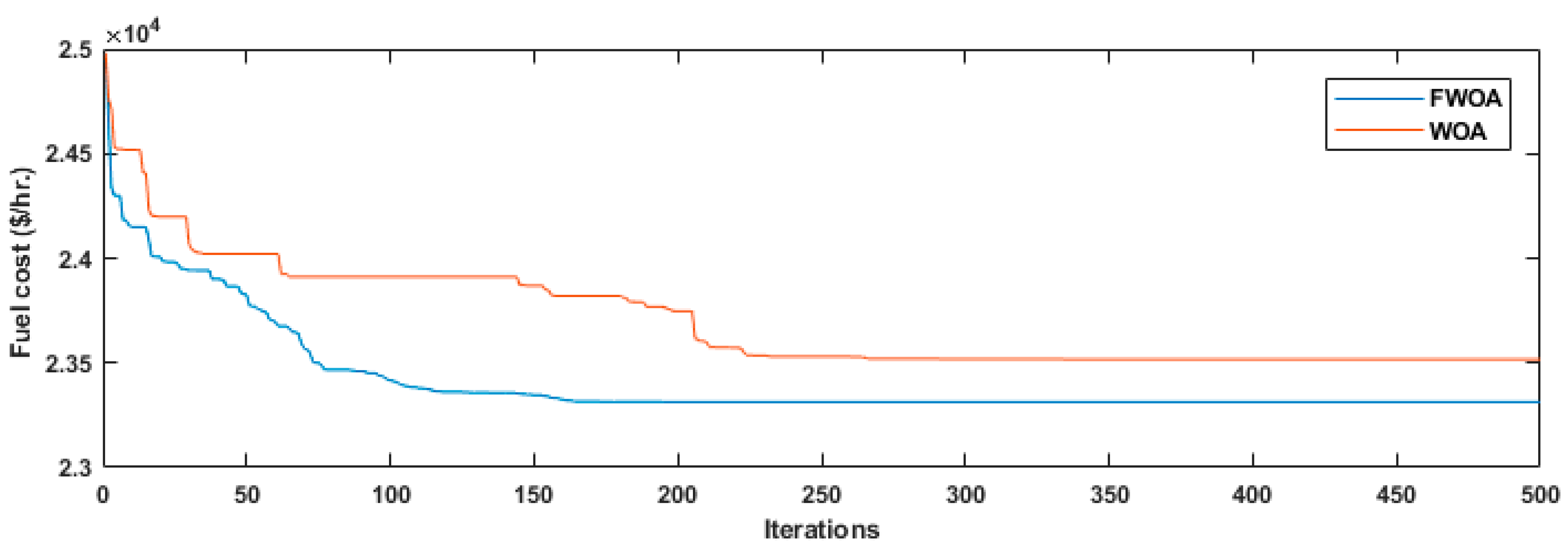
4.2. Case Study 2: Thirteen Thermal Generating Units Test System
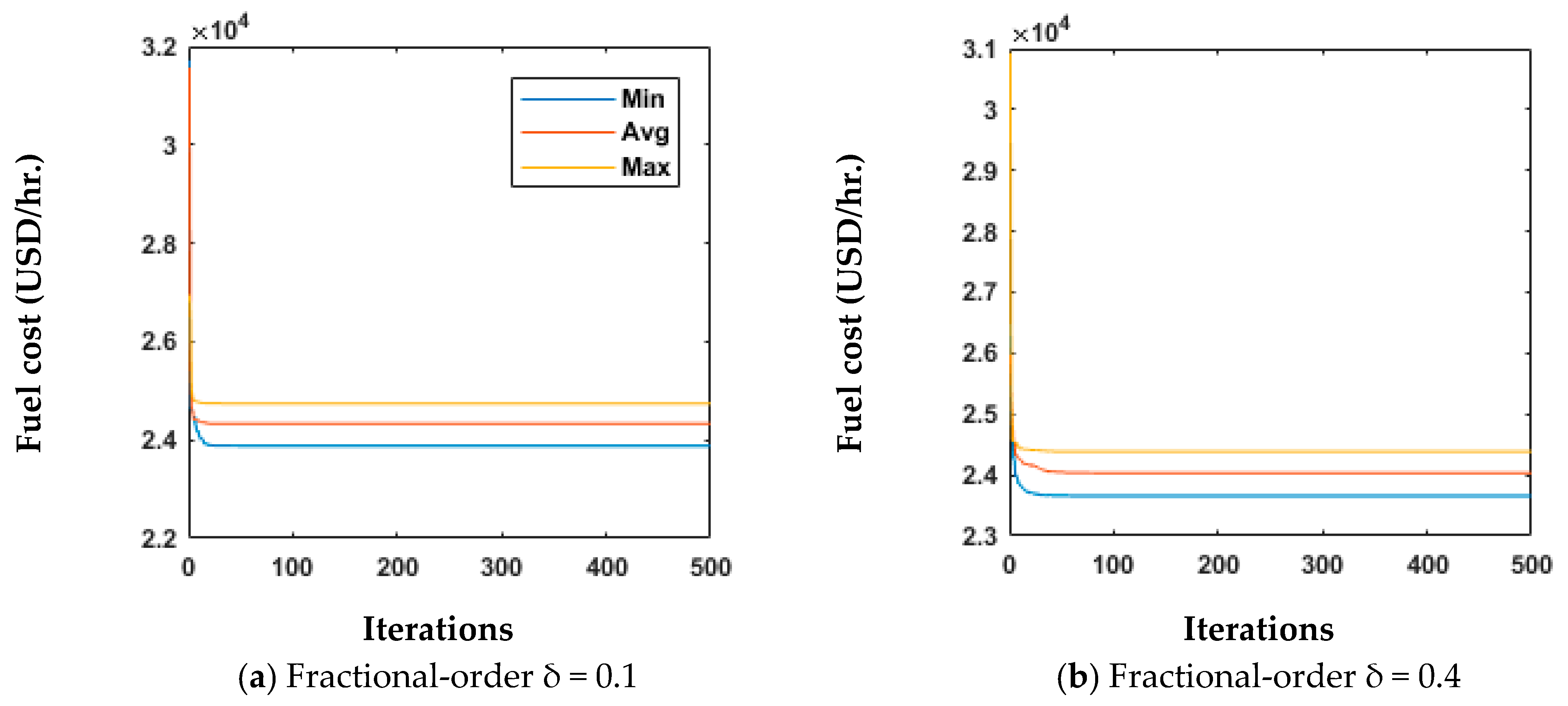
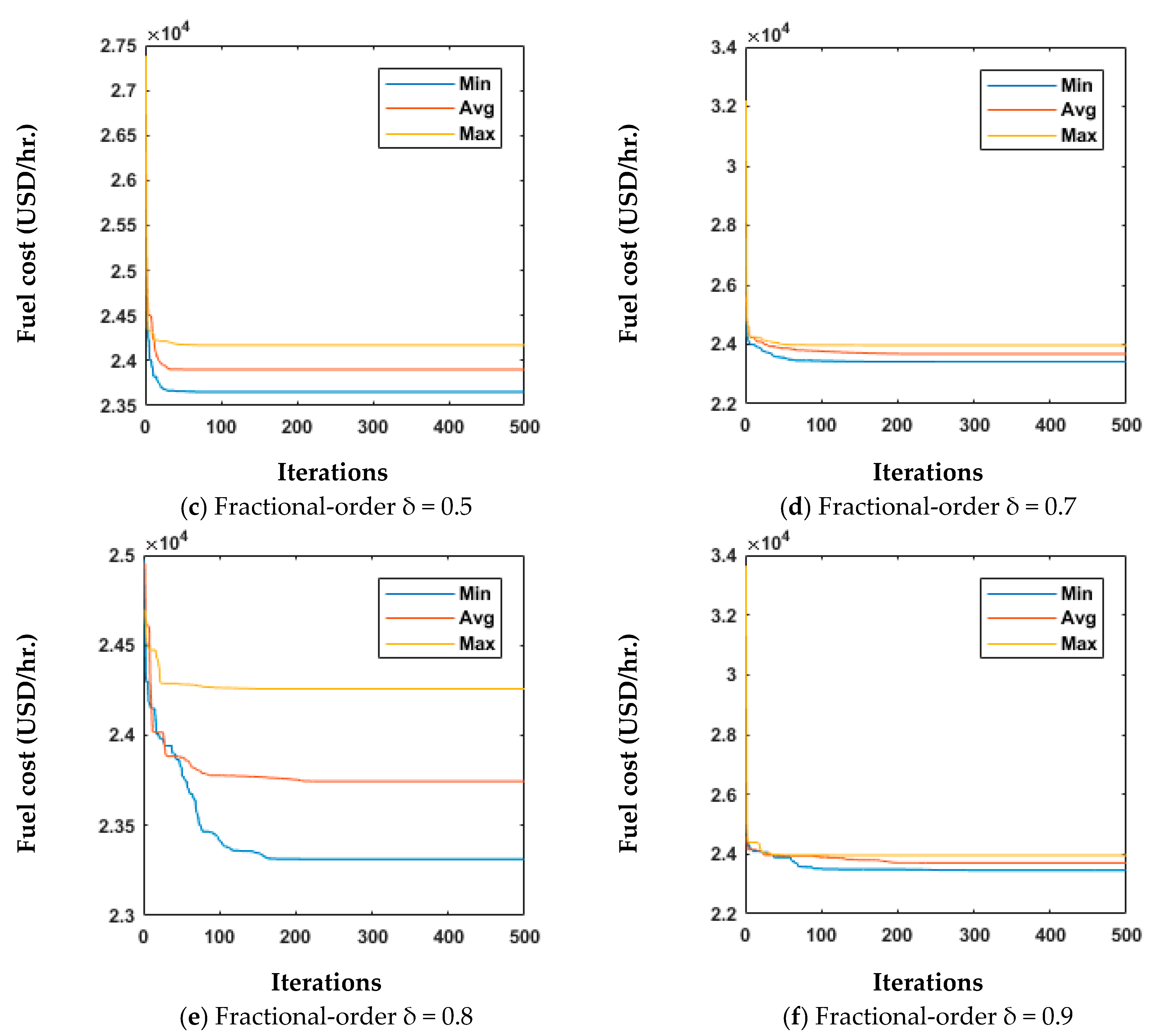
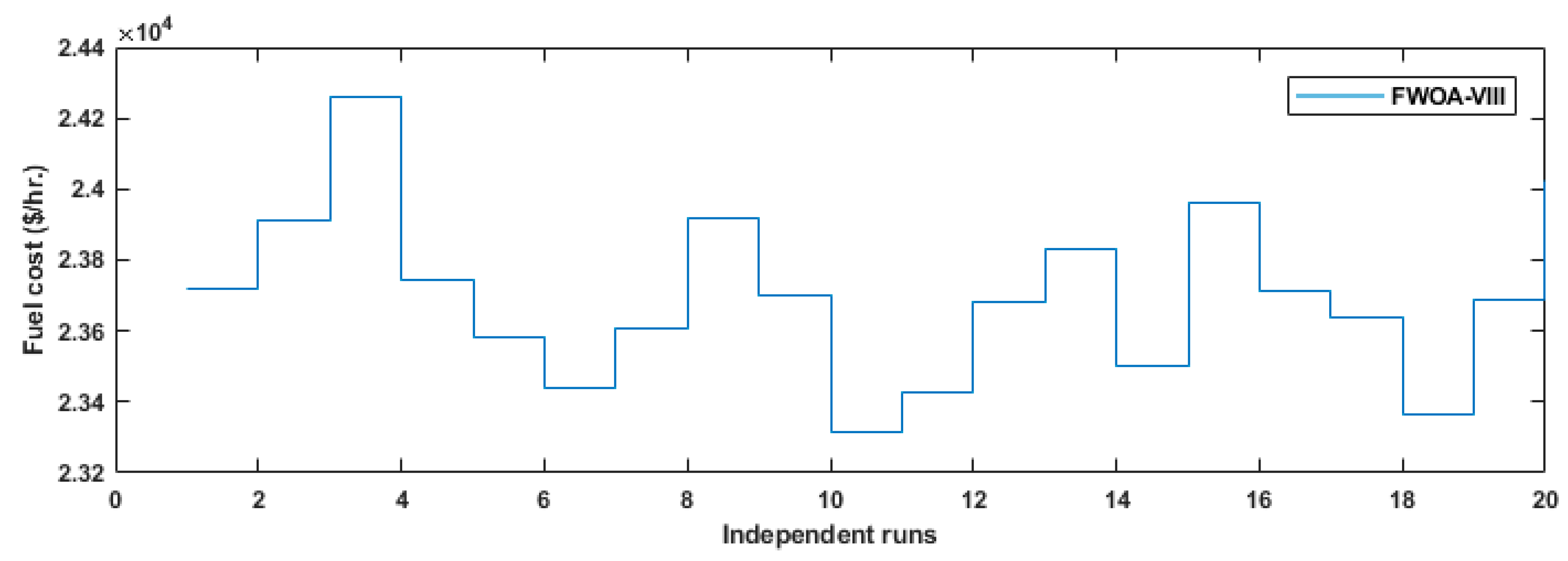
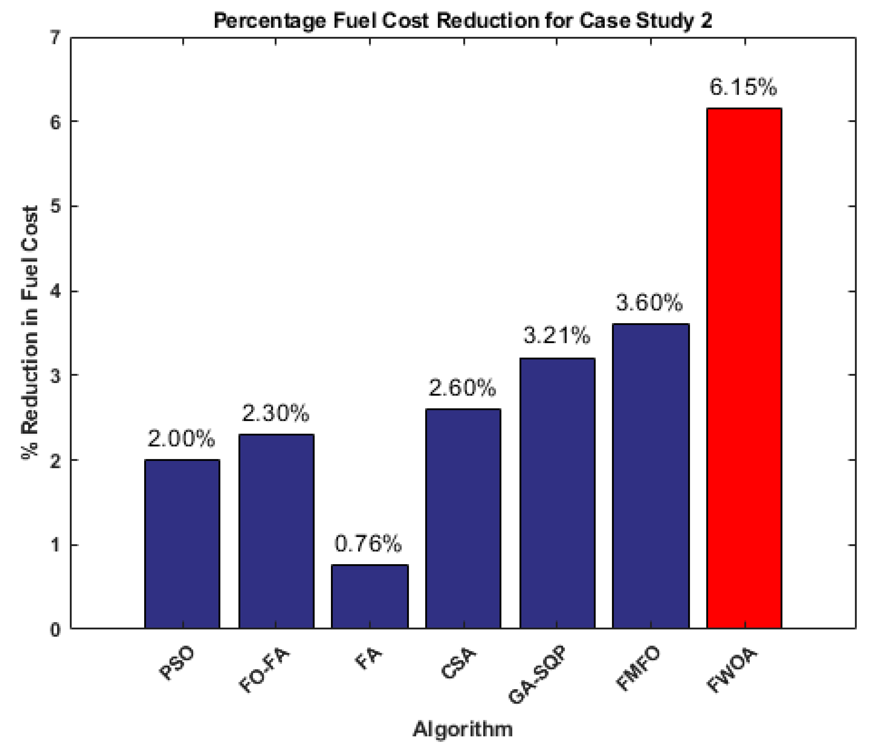
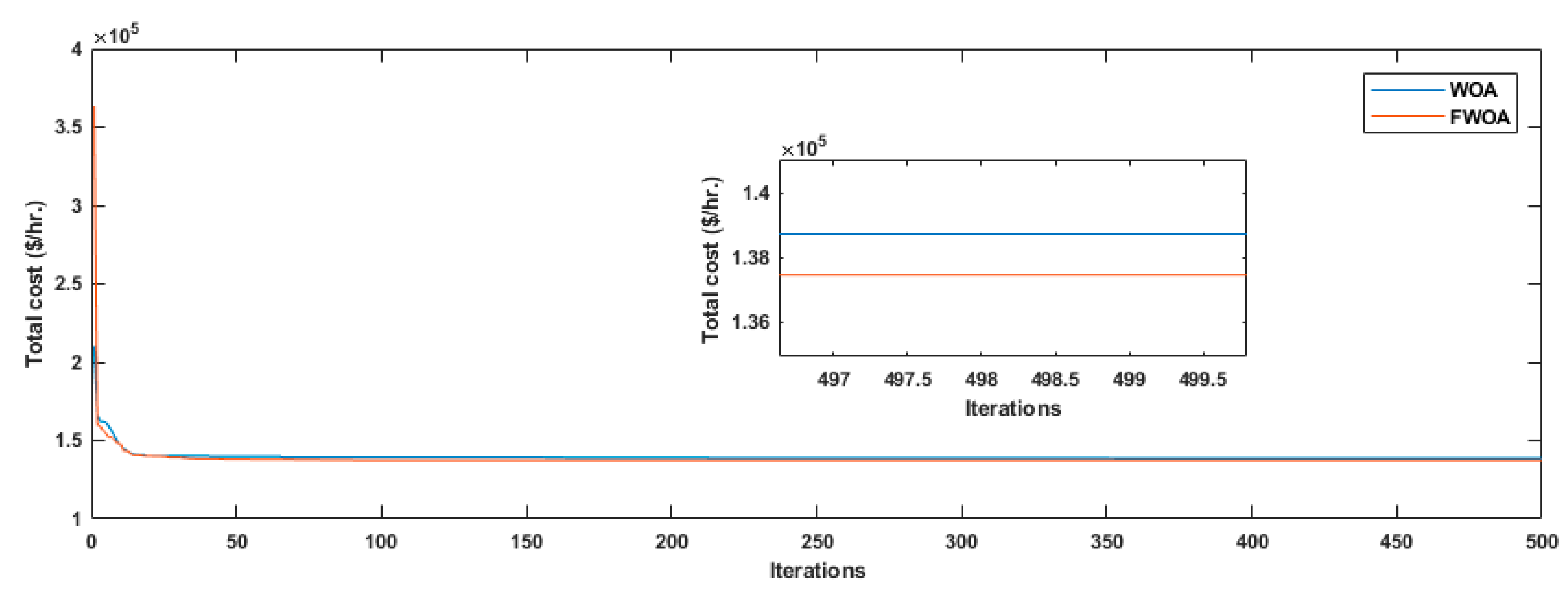
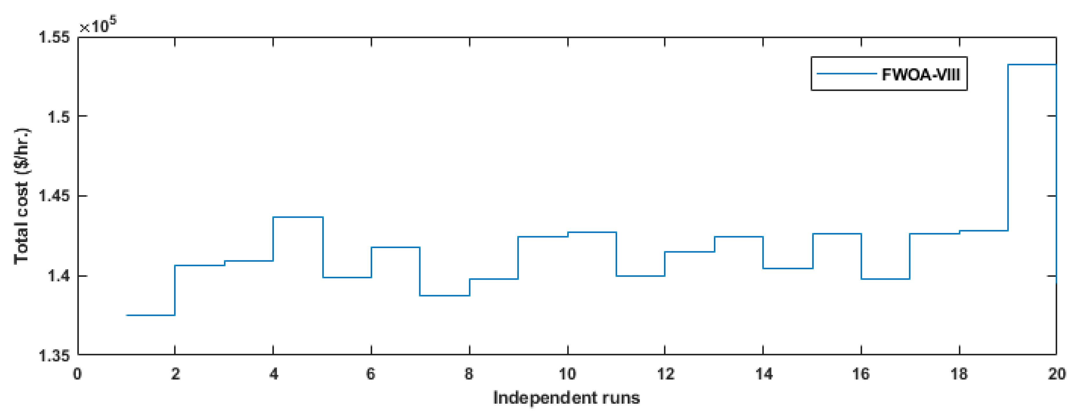
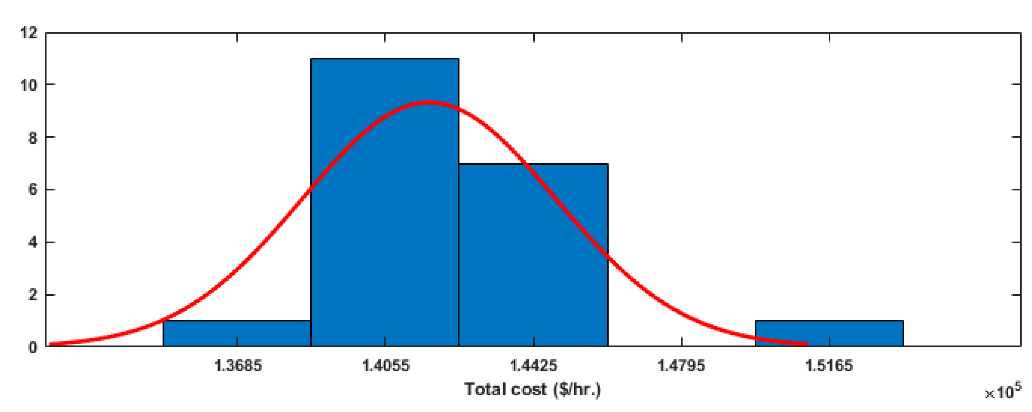
Case study 2 has a total of thirteen thermal power producing units. Thermal power generator fuel cost coefficients have been obtained from Ref. [1]. During case study 2, power demand is 2420 MW. The assessment of case study 2 utilizes 10 fractional order values that span from 0.1 to 0.9. The inherent randomness of the optimum simulation results produced by the FWOA technique should not be ignored. To meticulously test the extent of differences in optimized results, a total of 500 iterations were used to carry out 20 independent trials for each practice of the FWOA method. A simulation of the fuel cost value is shown in Table 5, (calculated in USD per hour) for each variation of the FWOA algorithm over 20 separate trials. Furthermore, Table 5 displays the numbers used to determine the factors related to the generation of active power in megawatts for the FWOA variants. The FWOA-VIII algorithm exhibits the most favorable simulation outcomes among the ten variants, specifically in terms of the minimal fuel generation cost of 23,313.53 USD per hour. Figure 7 demonstrates the efficacy of the concept by showcasing the convergence characteristics curve of FWOA-VIII compared to conventional WOA algorithm. Figure 8 shows convergence characteristic curves over a range of different fractional orders. Figure 9 and Figure 10 depict the 20 separate trials and histogram related to the most effective version of FWOA, especially FWOA-VIII. Table 6 provides a summary of the minimum fuel costs specified by FWOA and their most recent equivalents from the literature, such as PSO, FO-FA, FA, CSA, GA-SQP, FMFO [31], and the proposed FWOA. The percentage reduction in fuel cost includes 2% for PSO, 2.3% for FO-FA, 0.76% for FA, 2.6% for CSA, 3.21% for GA-SQP, 3.6% FMFO, and 6.15% for the proposed FWOA as shown in Figure 11.
Table 5.
Comparative assessment of the proposed FWOA algorithm for Case study 2.
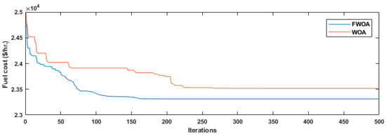
Figure 7.
Fitness curve of best variant FWOA-VIII for case study 2.
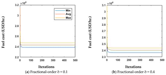
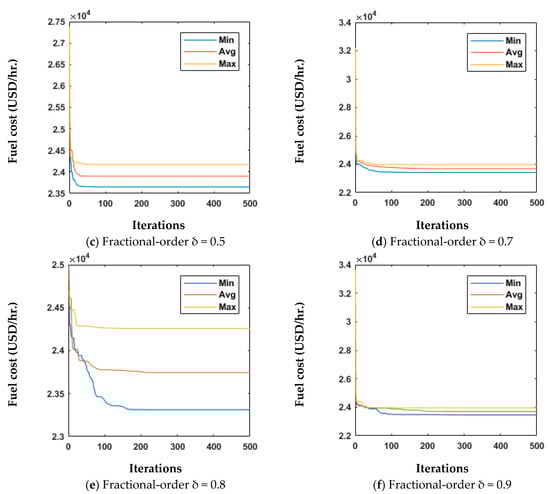
Figure 8.
Convergence characteristic curves of proposed FWOA algorithm in case of thirteen thermal generating units test system.
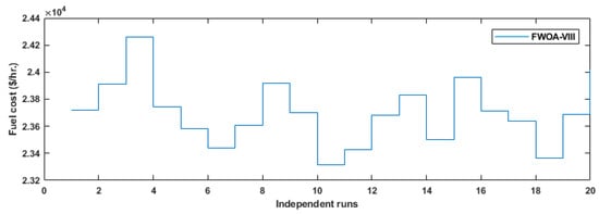
Figure 9.
Independent runs observations of variant FWOA-VIII for case study 2.
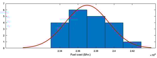
Figure 10.
Histogram observations of variant FWOA-VIII for case study 2.
Table 6.
Comparison of proposed FWOA algorithm with different solvers from literature for case study 2.

Figure 11.
Comparison of percentage fuel cost reduction for 13 generating units test system.
Case study 3: Taiwan 37 Thermal generating units integrated with 3 wind power units.
Case study 3 is carried out on the ELD-VPLE-SW problem, focusing on a group of 40 generators. Specifically, the investigation examines 37 thermal power generating units and the final 3 units of wind power generating units. The incorporation of SW into an ELD is achieved by the formulation of Equation (3) in the system model. Equation (10) is used to calculate the total generating cost. The system details regarding the wind and thermal unit can be found in Ref. [23]. Each version of the WOA algorithm (FWOA-I through FWOA-IX) underwent 20 independent trials, with 500 iterations in each. The algorithms i.e., FWOA-I to FWOA-IX, each consisted of 500 iterations. Table 7 displays the most favorable total cost in USD per hour for several versions of the FWOA algorithm. The variations range from a value of 0.1 to 0.9 in the fractional-order values with an increment of 0.1 in each step.
Table 7.
Comparative analysis of several versions of the FWOA algorithm for case study 3.
In comparison, the prominent simulation results for FWOA-VIII indicated a total cost of 137,472.4 USD per hour, comprised of 120,862.9542 USD per hour for fuel and 16,609.443 USD per hour for wind power. Figure 12 illustrates the learning curve for the FWOA-VIII variant along with conventional WOA, whereas the values for determining parameters in relation to real power generating yield in megawatts can be found in Table A1 and A2 of the Appendix A for the FWAO-I to FWOA-IX variants. Figure 13 and Figure 14 display the 20 independent trials and histogram pertaining to the optimal variant of WOA, specifically FWOA-VIII. Figure 15 shows convergence characteristic curves over a range of different fractional orders. The statistical results for fuel cost, expressed as means and standard deviations, are utilized in the analysis. The data provided in Table 8 are obtained from 20 separate trials for each variation. The average overall cost, as well as the standard deviation, decreases as the fractional order value increases.
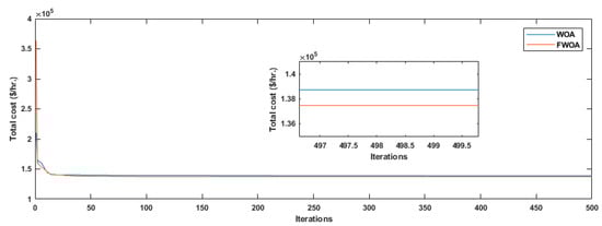
Figure 12.
Fitness curve of best variant FWOA-VIII.
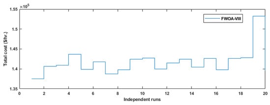
Figure 13.
Independent runs observations of variant FWOA-VIII for case study 3.
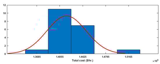
Figure 14.
Histogram observations of variant FWOA-VIII for case study 3.
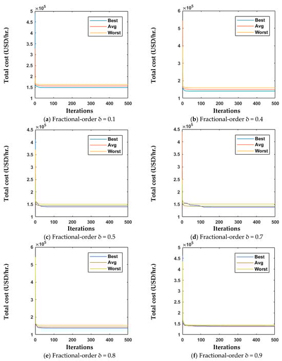
Figure 15.
Convergence characteristic curves of proposed FWOA algorithm in case of forty thermal generating units test system.
Table 8.
Statistical findings for total cost in terms of means and standard deviations for case study 3.
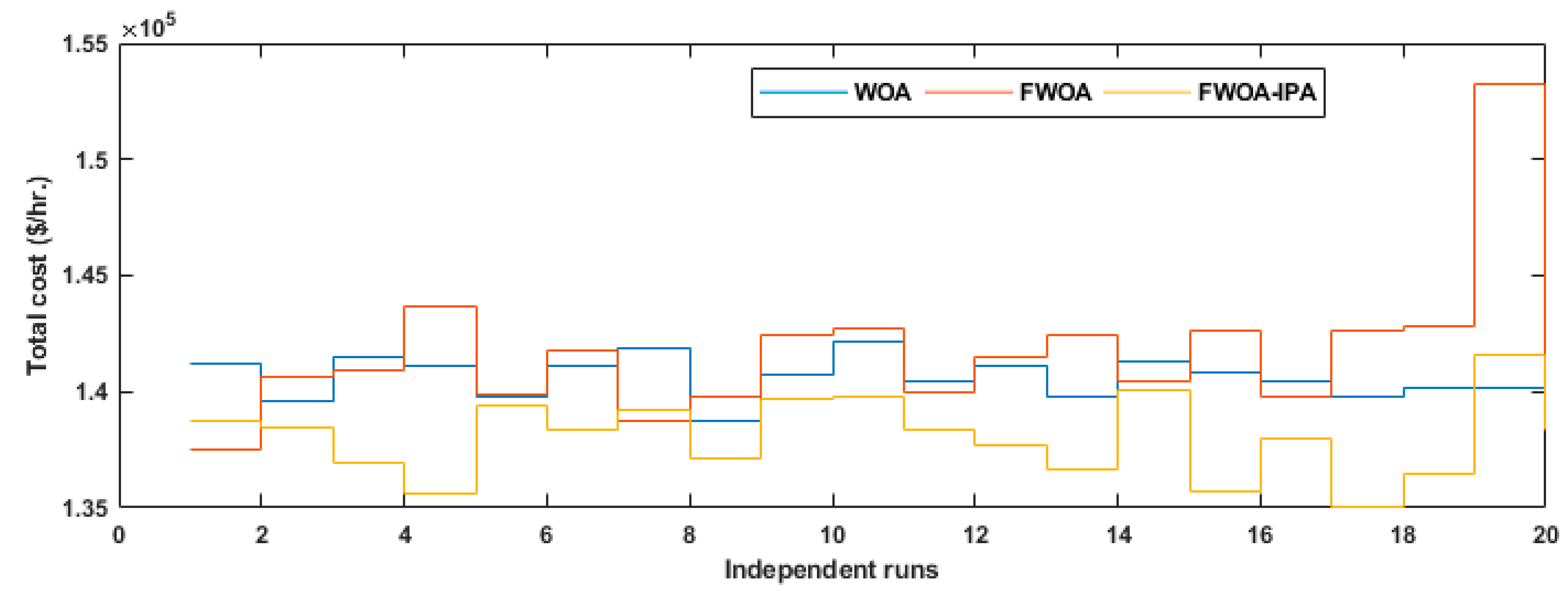
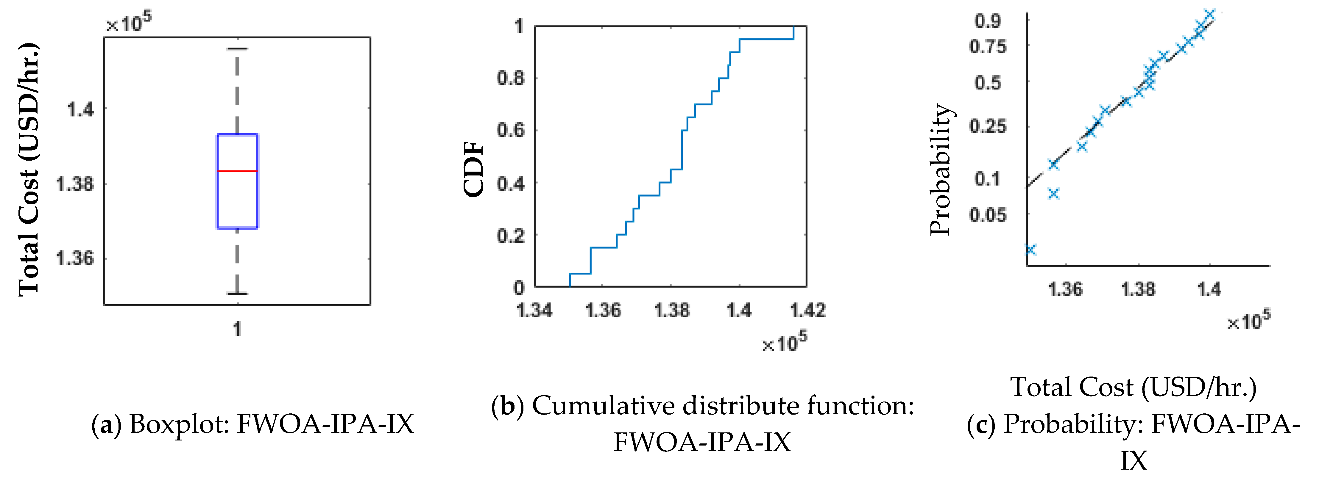
In addition, IPA was integrated into each variant of the FWOA algorithm (FWOA-I to WOA-IX) to improve the overall optimal results of FWOA. Table 9 displays the optimal results obtained for each hybridized variant of the FWOA algorithm out of 20 independent trials. FWOA-IPA-IX, a hybridized scheme methodology, produced superior convergence results at a total cost of 135,045.4390 USD per hour. The results from 20 separate trials for each scheme of hybridized FWOA variants were subjected to a statistical analysis using performance metrics. Figure 16 illustrates the aggregate expenditure incurred for 20 independent trials of the FWOA-IPA-IX variant along with FWOA and conventional WOA algorithm. The statistical performance indices, including function count (FC), total cost, iterations, and mean and standard deviations for time, were performed for each variant of the hybridized FWOA algorithm. The results obtained using the mean and standard deviation operators for fuel generation cost, computation time, iterations, and function counts for FWOA-IPA-IX are as follows: 0.89 ± 0.30, 115 ± 38, 9530 ± 3094, and 136,003.81741 ± 887.62, respectively. An investigation was performed for each hybridized variation of the FWOA algorithm using 20 separate trials to determine the overall generation cost. This analysis utilized statistical observations supported by CDF-based studies, boxplot, and histogram. Figure 17 and Figure 18 display the statistically derived observation plots for FWOA-IPA-IX. In histogram-based analysis, most independent trial data are found around the median value of the Gaussian fit. The study examines the accuracy of 20 separate trials with a chance of occurrence above 0.8 using CDF plots. The results of the comparison between the suggested form of FWOA hybridization with IPA and the most recent published ideas HIC-SQP [23], PWTED1 [43], and DWTED1 [43] for the ELD problem with VPLE incorporating SW impact were shown in Table 10. The optimal outcome was identified for the FWOA-IPA-1X, which incurred a total cost of 135,045.4390 USD per hour, comprised of 118,435.9957 USD for fuel and 16,609.4433 USD for wind energy. Figure 19 shows the fuel cost reduction percentages for several algorithms, including HIC-SQP (5%), PWTED1 (3.9%), DWTED1 (4.45%), GA-SQP (4.8%), PSO (3.19%), COOT (3.2%), and the suggested FWOA method (5.95%).
Table 9.
Comparison of hybridized variants of WOA algorithm for case study 3.
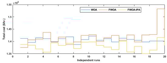
Figure 16.
Independent runs observations of variant WOA, FWOA, and FWOA-IPA for case study 3.
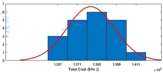
Figure 17.
Histogram observations of variant FWOA-IPA-IX for case study 3.
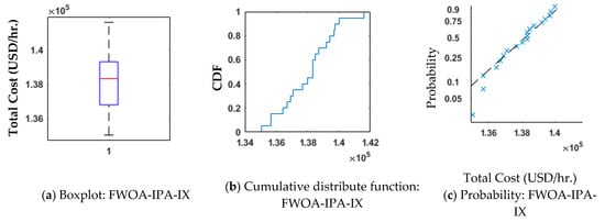
Figure 18.
Statistical observations of FWOA-IPA-IX algorithm for case study 3.
Table 10.
Comparison of proposed hybrid WOA algorithm for case study 3.
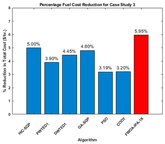
Figure 19.
Comparison of percentage fuel cost reduction for 40 generating units test system.
5. Conclusions
Concluding remarks are listed as follows.
- The total generation cost of hybrid energy generating units, which includes the costs of fuel generation and stochastically varying wind power, can be efficiently optimized using fractional order calculus. This optimization is achieved by utilizing the exploration and exploitation searching ability of the conventional WOA algorithm, which memorizes all past events and employs optimal mathematical modelling.
- Various variants of the proposed FWOA algorithm are utilized to evaluate its efficacy. Every set of FWOA variants is determined by the extent of the fractional order values ranging from 0.1 to 0.9. To achieve additional refinement, the local search-based algorithms IPA utilize the global outcomes of the FWOA algorithm as initial values. A total of three case studies have been considered to show the effectiveness of proposed scheme i-e case study 1 involves 3 thermal generating units test system, case 2 involves 13 thermal generating units test system, and case 3 involves 37 thermal generators and 3 wind power generators.
- For case study 1, the FWOA-IX variant produced a total fuel generation cost of 8194.376 USD per hour. The percentage fuel cost reduction of 0.23% for NSS, GA, GSA, GAB, and 0.22% for EP, whereas 0.71% fuel cost reduction was observed for the proposed FWOA.
- For case study 2, the FWOA-VIII variant produced a total fuel generation cost of 23,313.53 USD per hour. The percentage fuel cost reduction was 2% for PSO, 2.3% for FO-FA, 0.76% for FA, 2.6% for CSA, 3.21% for GA-SQP, and 3.6% for FMFO, whereas a 6.15% fuel cost reduction was observed for the proposed FWOA.
- For case study 3, the FWOA-IPA-IX variant produced a cost of 135,045.4390 USD per hour. The fuel cost reduction percentages for several algorithms, including HIC-SQP (5%), PWTED1 (3.9%), DWTED1 (4.45%), GA-SQP (4.8%), PSO (3.19%), COOT (3.2%), and the suggested FWOA method (5.95%), was observed for the proposed FWOA.
- The performance of the proposed case studies is evaluated using statistical, histogram, boxplot, and CDF-based analyses on the results of twenty independent trials for minimum objective function evaluation.
Author Contributions
Conceptualization, A.W., B.S.K., H.A. and A.M.A.; Methodology, A.W., B.S.K., H.A. and A.M.A.; Writing—Original draft, A.W. and B.S.K.; Writing—Review & editing, A.W., B.S.K., H.A. and A.M.A.; Supervision, A.W. and H.A.; Funding acquisition, H.A. and A.M.A. All authors have read and agreed to the published version of the manuscript.
Funding
This research was funded by the Deanship of Research and Graduate Studies at University of Tabuk for funding this work through Research no S-1444-0070.
Data Availability Statement
The data that support the findings of this study are available upon reasonable request from corresponding author.
Acknowledgments
The authors extend their appreciation to the Deanship of Research and Graduate Studies at University of Tabuk for funding this work through Research no S-1444-0070.
Conflicts of Interest
The authors declare no conflict of interest.
Appendix A
Best solutions of FWOA algorithm and its hybridized scheme for proposed case study are presented in Table A1 and Table A2.
Table A1.
Best solutions of FWOA algorithm for case study 3.
Table A1.
Best solutions of FWOA algorithm for case study 3.
| Units | FWOA-I | FWOA-II | FWOA-III | FWOA-IV | FWOA-V | FWOA-VI | FWOA-VII | FWOA-VIII | FWOA-IX |
|---|---|---|---|---|---|---|---|---|---|
| 1 | 114 | 114 | 114 | 114 | 114 | 114 | 114 | 114 | 114 |
| 2 | 114 | 114 | 114 | 114 | 114 | 114 | 114 | 114 | 114 |
| 3 | 120 | 60 | 120 | 120 | 60 | 101 | 110 | 105 | 120 |
| 4 | 80 | 190 | 190 | 190 | 190 | 190 | 190 | 190 | 190 |
| 5 | 97 | 97 | 97 | 97 | 97 | 97 | 97 | 97 | 97 |
| 6 | 140 | 140 | 140 | 140 | 140 | 140 | 140 | 139 | 140 |
| 7 | 300 | 300 | 300 | 300 | 300 | 300 | 291 | 300 | 300 |
| 8 | 300 | 300 | 300 | 300 | 300 | 284 | 300 | 300 | 300 |
| 9 | 300 | 300 | 300 | 284 | 300 | 300 | 300 | 300 | 300 |
| 10 | 130 | 130 | 130 | 130 | 130 | 130 | 130 | 130 | 130 |
| 11 | 94 | 94 | 94 | 94 | 94 | 94 | 94 | 94 | 96 |
| 12 | 94 | 94 | 94 | 94 | 94 | 94 | 94 | 94 | 94 |
| 13 | 125 | 125 | 125 | 125 | 125 | 125 | 125 | 125 | 125 |
| 14 | 393 | 321 | 305 | 125 | 125 | 125 | 306 | 303 | 307 |
| 15 | 394 | 218 | 300 | 215 | 397 | 215 | 306 | 305 | 305 |
| 16 | 125 | 301 | 125 | 500 | 296 | 500 | 125 | 125 | 125 |
| 17 | 500 | 500 | 500 | 500 | 500 | 500 | 500 | 500 | 488 |
| 18 | 500 | 500 | 500 | 500 | 500 | 500 | 500 | 500 | 500 |
| 19 | 550 | 550 | 550 | 550 | 550 | 550 | 550 | 550 | 550 |
| 20 | 550 | 550 | 550 | 504 | 511 | 508 | 550 | 550 | 550 |
| 21 | 550 | 550 | 550 | 550 | 550 | 550 | 550 | 550 | 540 |
| 22 | 550 | 550 | 550 | 549 | 550 | 530 | 550 | 550 | 550 |
| 23 | 550 | 550 | 550 | 550 | 550 | 550 | 550 | 550 | 550 |
| 24 | 550 | 550 | 550 | 550 | 550 | 550 | 550 | 550 | 550 |
| 25 | 550 | 550 | 550 | 542 | 550 | 550 | 550 | 550 | 550 |
| 26 | 550 | 522 | 550 | 550 | 550 | 524 | 550 | 550 | 550 |
| 27 | 97 | 87 | 97 | 97 | 97 | 97 | 96 | 97 | 97 |
| 28 | 190 | 190 | 190 | 190 | 190 | 190 | 190 | 190 | 190 |
| 29 | 190 | 190 | 190 | 190 | 190 | 190 | 190 | 190 | 190 |
| 30 | 190 | 190 | 190 | 190 | 190 | 190 | 190 | 190 | 190 |
| 31 | 200 | 200 | 200 | 198 | 200 | 200 | 200 | 200 | 200 |
| 32 | 200 | 200 | 200 | 198 | 200 | 200 | 200 | 200 | 200 |
| 33 | 200 | 200 | 200 | 166 | 200 | 200 | 200 | 200 | 200 |
| 34 | 25 | 110 | 110 | 110 | 110 | 110 | 110 | 110 | 110 |
| 35 | 110 | 110 | 110 | 96 | 110 | 110 | 110 | 110 | 110 |
| 36 | 110 | 85 | 110 | 110 | 108 | 110 | 110 | 110 | 110 |
| 37 | 550 | 550 | 537 | 550 | 550 | 550 | 550 | 550 | 550 |
| 38 | 18 | 18 | 18 | 18 | 18 | 18 | 18 | 18 | 18 |
| 39 | 46 | 46 | 46 | 46 | 46 | 46 | 46 | 46 | 46 |
| 40 | 54 | 54 | 54 | 54 | 54 | 54 | 54 | 54 | 54 |
| Power Demand | 10,500 | 10,500 | 10,500 | 10,500 | 10,500 | 10,500 | 10,500 | 10,500 | 10,500 |
Table A2.
Best solutions of FWOA algorithm hybrid with IPA for case study 3.
Table A2.
Best solutions of FWOA algorithm hybrid with IPA for case study 3.
| Units | FWOA-IPA-1 | FWOA-IPA-II | FWOA-IPA-III | FWOA-IPA-IV | FWOA-IPA-V | FWOA-IPA-VI | FWOA-IPA-VII | FWOA-IPA-VIII | FWOA-IPA-IX |
|---|---|---|---|---|---|---|---|---|---|
| 1 | 114 | 114 | 114 | 114 | 114 | 114 | 111 | 114 | 114 |
| 2 | 114 | 114 | 114 | 114 | 114 | 114 | 114 | 114 | 114 |
| 3 | 120 | 97 | 120 | 120 | 120 | 120 | 97 | 115 | 120 |
| 4 | 180 | 180 | 180 | 190 | 180 | 180 | 180 | 180 | 190 |
| 5 | 97 | 97 | 97 | 88 | 97 | 88 | 88 | 98 | 88 |
| 6 | 140 | 140 | 140 | 140 | 140 | 140 | 140 | 140 | 140 |
| 7 | 300 | 300 | 300 | 260 | 300 | 260 | 300 | 300 | 300 |
| 8 | 300 | 285 | 290 | 285 | 300 | 285 | 285 | 300 | 298 |
| 9 | 300 | 285 | 290 | 300 | 300 | 300 | 285 | 300 | 285 |
| 10 | 130 | 130 | 130 | 130 | 130 | 130 | 130 | 130 | 130 |
| 11 | 94 | 94 | 94 | 94 | 94 | 240 | 94 | 94 | 94 |
| 12 | 94 | 94 | 94 | 94 | 94 | 94 | 94 | 94 | 94 |
| 13 | 125 | 125 | 125 | 125 | 125 | 125 | 125 | 125 | 125 |
| 14 | 485 | 484 | 125 | 475 | 394 | 394 | 125 | 395 | 395 |
| 15 | 305 | 125 | 395 | 480 | 125 | 484 | 485 | 125 | 485 |
| 16 | 215 | 485 | 396 | 127 | 396 | 125 | 484 | 485 | 125 |
| 17 | 489 | 500 | 489 | 489 | 489 | 500 | 489 | 489 | 489 |
| 18 | 489 | 489 | 489 | 489 | 489 | 500 | 489 | 489 | 489 |
| 19 | 511 | 511 | 511 | 511 | 511 | 511 | 511 | 511 | 550 |
| 20 | 511 | 511 | 550 | 511 | 550 | 511 | 550 | 511 | 511 |
| 21 | 533 | 523 | 523 | 523 | 523 | 523 | 523 | 523 | 523 |
| 22 | 530 | 523 | 523 | 523 | 523 | 523 | 523 | 523 | 523 |
| 23 | 526 | 523 | 550 | 523 | 550 | 523 | 523 | 523 | 523 |
| 24 | 526 | 523 | 550 | 523 | 531 | 523 | 523 | 550 | 523 |
| 25 | 523 | 523 | 523 | 523 | 523 | 523 | 523 | 523 | 523 |
| 26 | 523 | 523 | 523 | 523 | 523 | 523 | 523 | 523 | 523 |
| 27 | 97 | 97 | 97 | 97 | 97 | 88 | 88 | 97 | 97 |
| 28 | 190 | 190 | 190 | 190 | 190 | 190 | 190 | 190 | 190 |
| 29 | 190 | 190 | 190 | 190 | 190 | 190 | 190 | 190 | 190 |
| 30 | 190 | 190 | 190 | 190 | 190 | 190 | 190 | 190 | 190 |
| 31 | 200 | 200 | 200 | 200 | 200 | 200 | 200 | 200 | 200 |
| 32 | 200 | 200 | 200 | 200 | 200 | 165 | 165 | 200 | 200 |
| 33 | 200 | 175 | 200 | 200 | 200 | 165 | 165 | 200 | 200 |
| 34 | 110 | 110 | 110 | 110 | 110 | 110 | 110 | 110 | 110 |
| 35 | 110 | 110 | 110 | 110 | 110 | 110 | 110 | 110 | 110 |
| 36 | 110 | 110 | 110 | 110 | 110 | 110 | 110 | 110 | 110 |
| 37 | 511 | 512 | 550 | 511 | 550 | 511 | 550 | 511 | 511 |
| 38 | 18 | 18 | 18 | 18 | 18 | 18 | 18 | 18 | 18 |
| 39 | 46 | 46 | 46 | 46 | 46 | 46 | 46 | 46 | 46 |
| 40 | 54 | 54 | 54 | 54 | 54 | 54 | 54 | 54 | 54 |
| Power Demand | 10,500 | 10,500 | 10,500 | 10,500 | 10,500 | 10,500 | 10,500 | 10,500 | 10,500 |
References
- Qu, B.-Y.; Zhu, Y.; Jiao, Y.; Wu, M.; Suganthan, P.N.; Liang, J. A survey on multi-objective evolutionary algorithms for the solution of the environmental/economic dispatch problems. Swarm Evol. Comput. 2018, 38, 1–11. [Google Scholar] [CrossRef]
- Lin, C.E.; Viviani, G.L. Hierarchical Economic Dispatch for Piecewise Quadratic Cost Functions. IEEE Trans. Power Appar. Syst. 1984, PAS-103, 1170–1175. [Google Scholar] [CrossRef]
- Parikh, J.; Chattopadhyay, D. A multi-area linear programming approach for analysis of economic operation of the Indian power system. IEEE Trans. Power Syst. 1996, 11, 52–58. [Google Scholar] [CrossRef]
- Zhu, J.; Momoh, J.A. Multi-area power systems economic dispatch using nonlinear convex network flow programming. Electr. Power Syst. Res. 2001, 59, 13–20. [Google Scholar] [CrossRef]
- Ding, T.; Bo, R.; Li, F.; Sun, H. A bi-level branch and bound method for economic dispatch with disjoint prohibited zones considering network losses. IEEE Trans. Power Syst. 2014, 30, 2841–2855. [Google Scholar] [CrossRef]
- El-Keib, A.; Ma, H.; Hart, J. Environmentally constrained economic dispatch using the LaGrangian relaxation method. IEEE Trans. Power Syst. 1994, 9, 1723–1729. [Google Scholar] [CrossRef]
- He, X.S.; Fan, Q.-W.; Karamanoglu, M.; Yang, X.-S. Comparison of constraint-handling techniques for metaheuristic optimization. In Proceedings of the International Conference on Computational Science, Faro, Portugal, 12–14 June 2019; Springer: Berlin/Heidelberg, Germany, 2019; pp. 357–366. [Google Scholar]
- Powell, D.; Skolnick, M.M. Using genetic algorithms in engineering design optimization with non-linear constraints. In Proceedings of the 5th International conference on Genetic Algorithms, Urbana-Champaign, IL, USA, 17–21 July 1993; pp. 424–431. [Google Scholar]
- Runarsson, T.; Yao, X. Stochastic ranking for constrained evolutionary optimization. IEEE Trans. Evol. Comput. 2000, 4, 284–294. [Google Scholar] [CrossRef]
- Takahama, T.; Sakai, S. Solving constrained optimization problems by the econstrained particle swarm optimizer with adaptive velocity limit control. In Proceedings of the 2006 IEEE Conference on Cybernetics and Intelligent Systems, Bangkok, Thailand, 7–9 June 2006; IEEE: Piscataway, NJ, USA, 2006; pp. 1–7. [Google Scholar]
- Yu, X.; Yu, X.; Lu, Y.; Sheng, J. Economic and emission dispatch using ensemble multi-objective differential evolution algorithm. Sustainability 2018, 10, 418. [Google Scholar] [CrossRef]
- Jiang, S.; Ji, Z.; Wang, Y. A novel gravitational acceleration enhanced particle swarm optimization algorithm for wind–thermal economic emission dispatch problem considering wind power availability. Int. J. Electr. Power Energy Syst. 2015, 73, 1035–1050. [Google Scholar] [CrossRef]
- Jadoun, V.K.; Pandey, V.C.; Gupta, N.; Niazi, K.R.; Swarnkar, A. Integration of renewable energy sources in dynamic economic load dispatch problem using an improved fireworks algorithm. IET Renew. Power Gener. 2018, 12, 1004–1011. [Google Scholar] [CrossRef]
- Chopra, L.; Kaur, R. Economic load dispatch using simple and refined genetic algorithm. Int. J. Adv. Eng. Technol. 2012, 5, 584–590. [Google Scholar]
- Gopalakrishnan, R.; Krishnan, A. An efficient technique to solve combined economic and emission dispatch problem using modified Ant colony optimization. Sadhana 2013, 38, 545–556. [Google Scholar] [CrossRef]
- Sinha, N.; Chakrabarti, R.; Chattopadhyay, P. Evolutionary programming techniques for economic load dispatch. IEEE Trans. Evol. Comput. 2003, 7, 83–94. [Google Scholar] [CrossRef]
- Balamurugan, K.; Muralisachithnndam, R.; Krishnan, S.R. Differential evolution based solution for combined economic and emission power dispatch with valve loading effect. Int. J. Electr. Eng. Inform. 2014, 6, 74. [Google Scholar] [CrossRef]
- Santra, D.; Sarker, K.; Mukherjee, A.; Mondal, S. Combined economic emission and load dispatch using hybrid metaheuristics. Int. J. Hybrid Intell. 2019, 1, 211–238. [Google Scholar] [CrossRef]
- Senthil, K.; Manikandan, K. Economic Thermal Power Dispatch with Emission Constraint and Valve Point Effect Loading Using Improved Tabu Search Algorithm. Int. J. Comput. Appl. 2010, 3, 6–11. [Google Scholar] [CrossRef]
- Jeyakumar, D.N.; Jayabarathi, T.; Raghunathan, T. Particle swarm optimization for various types of economic dispatch problems. Int. J. Electr. Power Energy Syst. 2006, 28, 36–42. [Google Scholar] [CrossRef]
- Pandit, M.; Chaudhary, V.; Dubey, H.M.; Panigrahi, B. Multi-period wind integrated optimal dispatch using series PSO-DE with time-varying Gaussian membership function based fuzzy selection. Int. J. Electr. Power Energy Syst. 2015, 73, 259–272. [Google Scholar] [CrossRef]
- Eberhart, R.; Kennedy, J. A new optimizer using particle swarm theory. In Proceedings of the Sixth International Symposium on Micro Machine and Human Science (MHS’95), Nagoya, Japan, 4–6 October 1995; IEEE: Piscataway, NJ, USA, 1995; pp. 39–43. [Google Scholar]
- Morshed, M.J.; Asgharpour, A. Hybrid imperialist competitive-sequential quadratic programming (HIC-SQP) algorithm for solving economic load dispatch with incorporating stochastic wind power: A comparative study on heuristic optimization techniques. Energy Convers. Manag. 2014, 84, 30–40. [Google Scholar] [CrossRef]
- Ghamisi, P.; Couceiro, M.S.; Benediktsson, J.A. A Novel Feature Selection Approach Based on FODPSO and SVM. IEEE Trans. Geosci. Remote Sens. 2014, 53, 2935–2947. [Google Scholar] [CrossRef]
- Ates, A.; Alagoz, B.B.; Kavuran, G.; Yeroglu, C. Implementation of fractional order filters discretized by modified Fractional Order Darwinian Particle Swarm Optimization. Measurement 2017, 107, 153–164. [Google Scholar] [CrossRef]
- Couceiro, M.S.; Rocha, R.P.; Ferreira, N.F.; Machado, J.T. Introducing the fractional-order Darwinian PSO. Signal Image Video Process. 2012, 6, 343–350. [Google Scholar] [CrossRef]
- Shahri, E.S.A.; Alfi, A.; Machado, J.T. Fractional fixed-structure H∞ controller design using augmented Lagrangian particle swarm optimization with fractional order velocity. Appl. Soft Comput. 2019, 77, 688–695. [Google Scholar] [CrossRef]
- Machado, J.T.; Kiryakova, V. The chronicles of fractional calculus. Fract. Calc. Appl. Anal. 2017, 20, 307–336. [Google Scholar] [CrossRef]
- Kuttomparambil Abdulkhader, H.; Jacob, J.; Mathew, A.T. Fractional-order lead-lag compensator-based multi-band power system stabiliser design using a hybrid dynamic GA-PSO algorithm. IET Gener. Transm. Distrib. 2018, 12, 3248–3260. [Google Scholar] [CrossRef]
- Kosari, M.; Teshnehlab, M. Non-linear fractional-order chaotic systems identification with approximated fractional-order derivative based on a hybrid particle swarm optimization-genetic algorithm method. J. AI Data Min. 2018, 6, 365–373. [Google Scholar]
- Khan, B.S.; Qamar, A.; Wadood, A.; Almuhanna, K.; Al-Shamma, A.A. Integrating economic load dispatch information into the blockchain smart contracts based on the fractional-order swarming optimizer. Front. Energy Res. 2024, 12, 1350076. [Google Scholar] [CrossRef]
- Wadood, A.; Park, H. A Novel Application of Fractional Order Derivative Moth Flame Optimization Algorithm for Solving the Problem of Optimal Coordination of Directional Overcurrent Relays. Fractal Fract. 2024, 8, 251. [Google Scholar] [CrossRef]
- Wadood, A.; Ahmed, E.; Rhee, S.B.; Sattar Khan, B. A Fractional-Order Archimedean Spiral Moth–Flame Optimization Strategy to Solve Optimal Power Flows. Fractal Fract. 2024, 8, 225. [Google Scholar] [CrossRef]
- Mirjalili, S.; Lewis, A. The whale optimization algorithm. Adv. Eng. Softw. 2016, 95, 51–67. [Google Scholar] [CrossRef]
- Potra, F.A.; Wright, S.J. Interior-point methods. J. Comput. Appl. Math. 2000, 124, 281–302. [Google Scholar] [CrossRef]
- Teodoro, G.S.; Machado, J.T.; de Oliveira, E.C. A review of definitions of fractional derivatives and other operators. J. Comput. Phys. 2019, 388, 195–208. [Google Scholar] [CrossRef]
- Sabatier, J.A.T.M.J.; Agrawal, O.P.; Machado, J.T. Advances in Fractional Calculus; Springer: Dordrecht, The Netherlands, 2007; Volume 4. [Google Scholar]
- Kamboj, V.K.; Bath, S.; Kand Dhillon, J.S. Solution of non-convex economic load dispatch problem using Grey Wolf Optimizer. Neural Comput. Appl. 2016, 27, 1301–1316. [Google Scholar] [CrossRef]
- Tsai, M.T.; Gow, H.J.; Lin, W.M. A novel stochastic search method for the solution of economic dispatch problems with nonconvex fuel cost functions. Int. J. Electr. Power Energy Syst. 2011, 33, 1070–1076. [Google Scholar] [CrossRef]
- Duman, S.; Güvenç, U.; Yörükeren, N. Gravitational search algorithm for economic dispatch with valve-point effects. Int. Rev. Electr. Eng. 2010, 5, 2890–2895. [Google Scholar]
- Subhani, T.M.; Babu, C.S.; Reddy, A.S. Particle swarm optimization with time varying acceleration coefficients for economic dispatch considering valve point loading effects. In Proceedings of the 2012 Third International Conference on Computing, Communication and Networking Technologies (ICCCNT′12), Kharagpur, India, 6–8 July 2021; IEEE: Piscataway, NJ, USA, 2012; pp. 1–8. [Google Scholar]
- Mehmood, A.; Raja, M.A.Z.; Jalili, M. Optimization of integrated load dispatch in multi-fueled renewable rich power systems using fractal firefly algorithm. Energy 2023, 278, 127792. [Google Scholar] [CrossRef]
- Khan, B.S.; Raja, M.A.Z.; Qamar, A.; Chaudhary, N.I. Design of moth flame optimization heuristics for integrated power plant system containing stochastic wind. Appl. Soft Comput. 2021, 104, 107193. [Google Scholar] [CrossRef]


Disclaimer/Publisher’s Note: The statements, opinions and data contained in all publications are solely those of the individual author(s) and contributor(s) and not of MDPI and/or the editor(s). MDPI and/or the editor(s) disclaim responsibility for any injury to people or property resulting from any ideas, methods, instructions or products referred to in the content. |
© 2024 by the authors. Licensee MDPI, Basel, Switzerland. This article is an open access article distributed under the terms and conditions of the Creative Commons Attribution (CC BY) license (https://creativecommons.org/licenses/by/4.0/).