
A Piecewise Linear Approach for Implementing Fractional-Order Multi-Scroll Chaotic Systems on ARMs and FPGAs


 ,
,  ,
, 
Abstract
:1. Introduction
- Extra-degree of fredom. The most significant advantage of fractional-order systems is the extra degree of freedom provided by the non-integer order derivatives. This additional parameter allows for greater flexibility in modeling and control. In applications such as chaos synchronization, it is possible to tune and optimize the system behavior by varying the fractional order, thereby achieving precise synchronization schemes and control outcomes [18].
- Memory Properties and Hereditary Characteristics. Fractional-order systems possess memory properties and hereditary characteristics, which are absent in integer-order systems. These properties enhance the modeling of systems with memory effects and improve the effectiveness of chaos-based applications. For instance, the memory effects can introduce additional layers of complexity and unpredictability to the chaotic behavior, which can be used to create robust security applications [19,20].
- Larger Key-space. Fractional-order chaotic systems offer a significantly larger keyspace compared to integer-order systems due to the additional degrees of freedom provided by the fractional derivatives [21].
- Piecewise linear (PWL) functions. The reported digital implementations are predominantly based on fractional-order systems with quadratic functions, cubic functions, or quadratic cross-product functions. This could be caused because determining Adomian polynomials of complex functions is challenging [73]. Even when there are approaches to efficiently compute the Adomian polynomials of trigonometric, exponential, and logarithmic functions [59,74]; and improved ADM versions [75,76,77,78]; they still cannot represent PWL functions.
- Multi-scroll chaotic attractors. The informed physical implementations of chaotic systems using ADM are mostly confined to one-and two-scroll attractors. Indeed, the classical ADM does not cope with PWL functions, which are a fundamental mechanism to get multi-scroll chaotic attractors [79,80,81,82,83]. Thus, a relevant open problem is how to incorporate fractional-order dynamical systems based on PWL functions in the sense of ADM.
2. Background
3. Proposed Piecewise Linear Decomposition Method (PWL-DM Approach)
- is repeated once.
- is repeated times.
Convergence Analysis
4. Illustrative Example
4.1. Example 1: Step-by-Step Demonstration for a 2-scroll PWL Chaotic System
- Using PWL-DM
4.2. Example 2: 1D Multiscroll PWL Chaotic System
- Using PWL-DM
4.3. Example 3: 2D Grid Multi-Scroll PWL Chaotic System
- Using PWL-DM
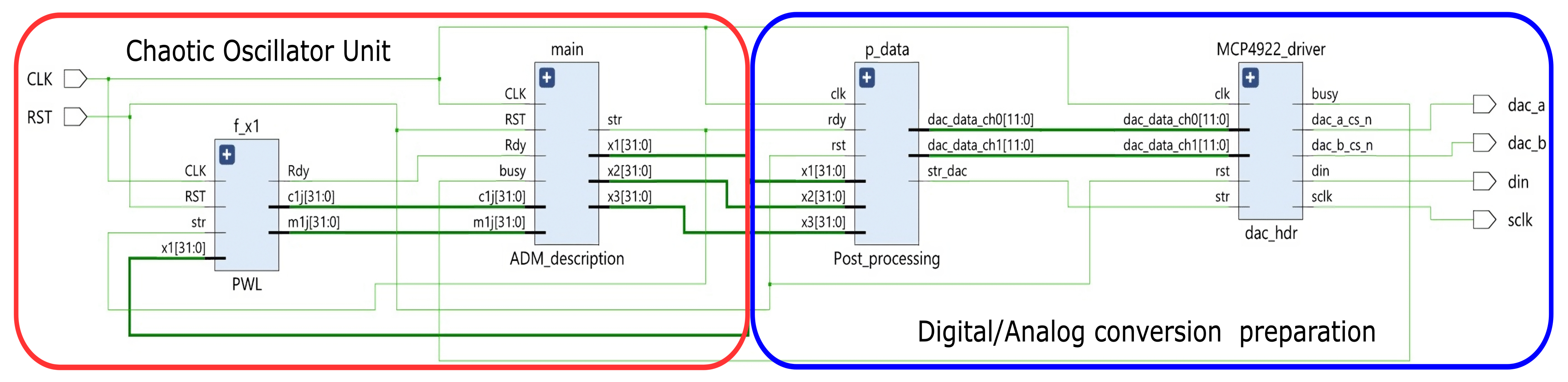
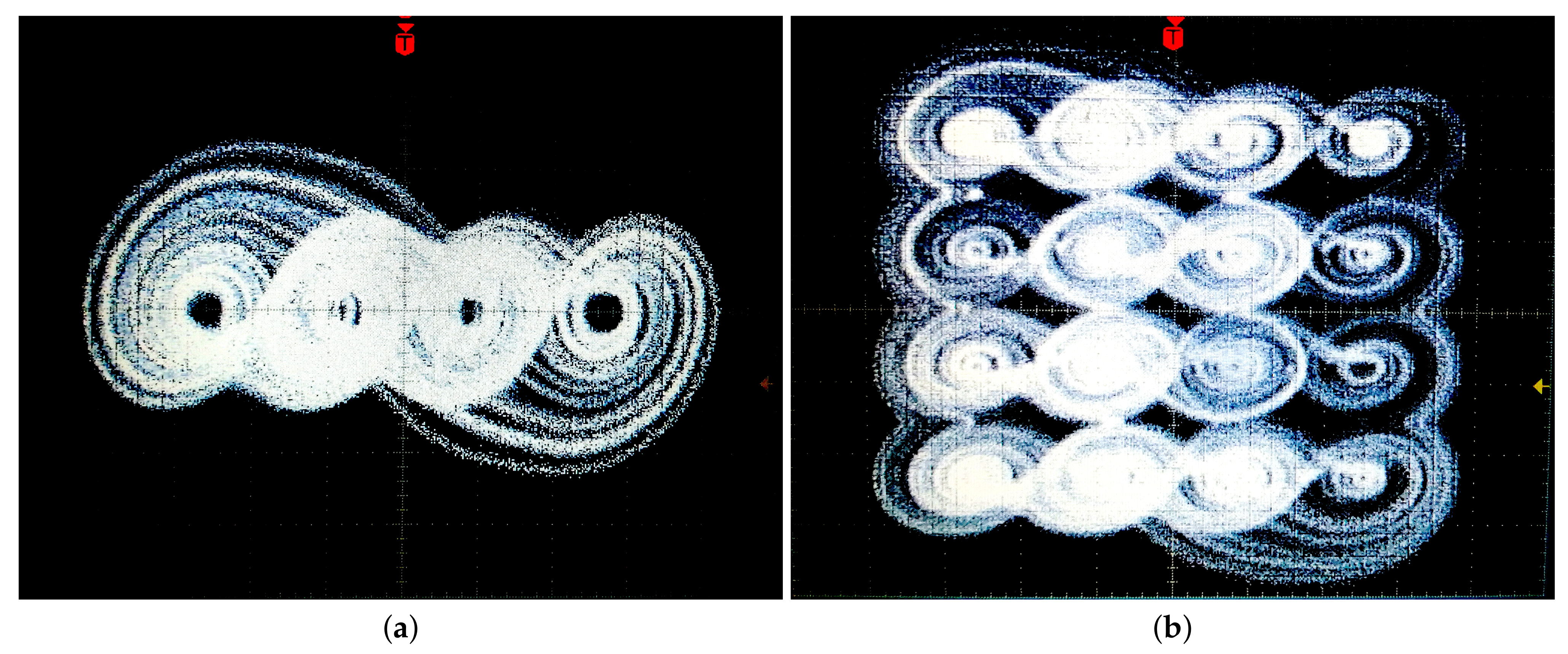
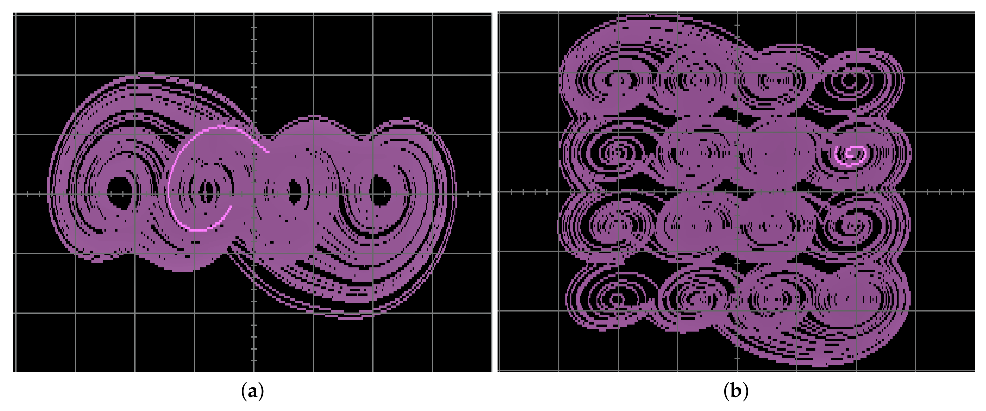
5. Physical Implementation of the PWL-DM Based on FPGA and ARM Digital Boards
5.1. Non-Embedded Design: PWL-DM Implementation Based on FPGA
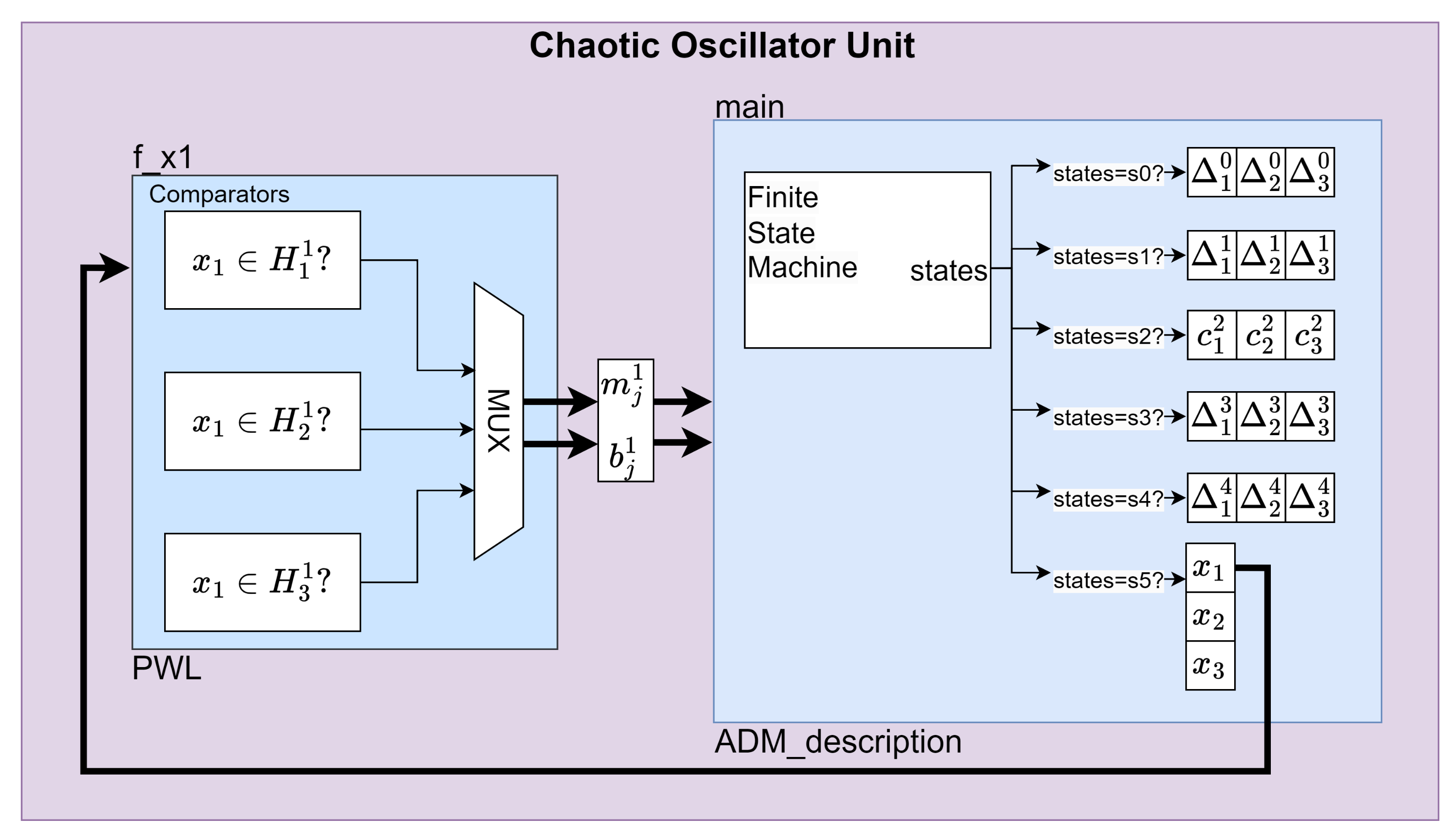
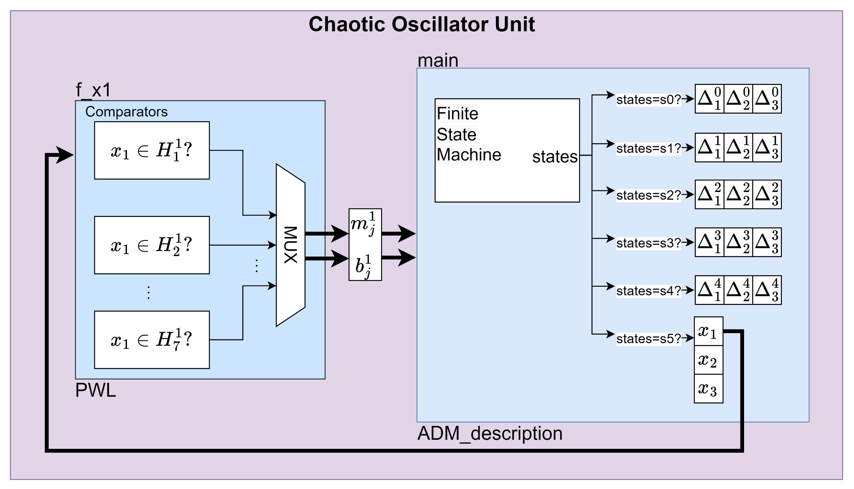
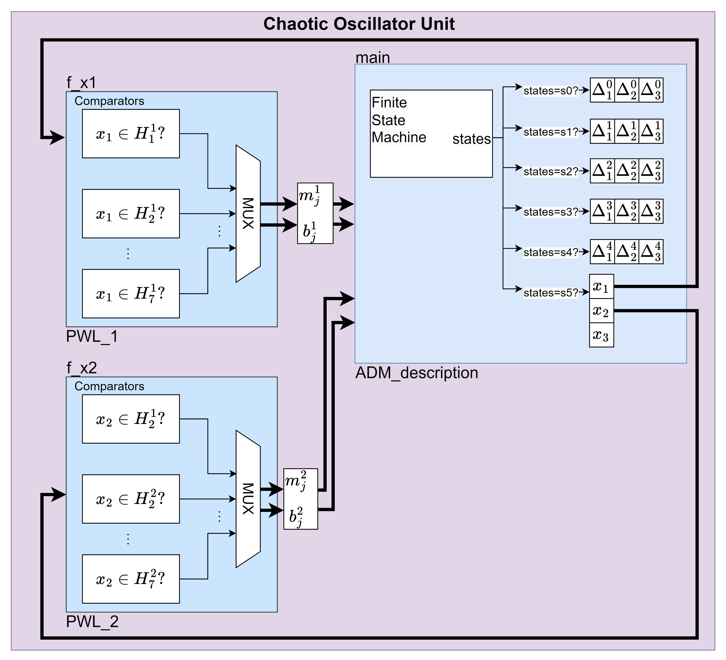
- Chaotic Oscillator Unit: The elements of the FPGA implementation for the , and scrolls are marked in color red. The highest level of the FPGA design for the and -scrolls (see Figure 7) comprises two blocks, whereas the -scrolls (see Figure 8) contains three blocks, each one performs calculations separately. The PWL blocks that describe the PWL function (Equations (28), (51) and (65)) are shown in Figure 9. Finally, the ADM_description block executes the proposed PWL-DM (20).
- Digital/Analog conversion: For visualization of the chaotic attractors on an oscilloscope, the Post_processing and dac_hdr blocks (blue square in Figure 7 and Figure 8), control the 12-bit dual-channel D/A converter MCP4922 at 20 MHz. It is worth remembering that both blocks may be deleted in practical applications, i.e., they should not be considered as part of the final implementation since they are just used for visualization purposes.
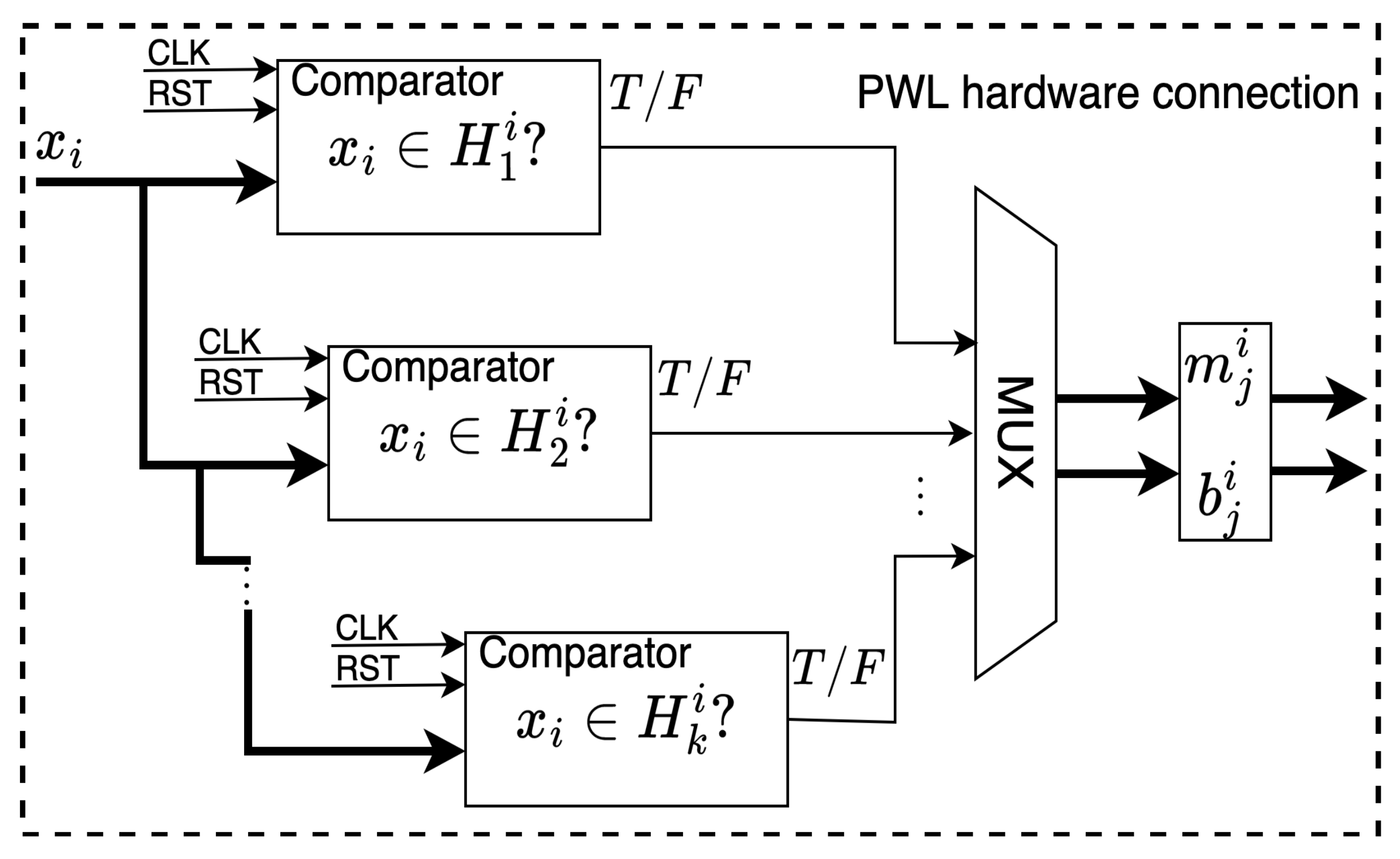
- 1D 2-scrolls generation mechanism
- Signal Comparison. The signal is compared against the predefined regions , and .
- Multiplexer (MUX). Based on the comparison results, the MUX selects appropriate values for the parameters and .
- PWL-DM Description. The parameters and are fed into the ADM_description block, which uses a Finite State Machine (FSM) that transitions from state to state . Each state processes parallel calculations corresponding to a set of coefficients . In state , the calculation results of the coefficients are used to calculate the solution of the system and hence to generate a 2-scroll chaotic attractor.
- 1D 4-scrolls generation mechanism
- Extended Signal Comparison. The signal is compared against more regions, from to , to determine which parameters to use.
- Expanded MUX. The MUX block is expanded to handle the additional regions and selects appropriate parameters , for generating a 4-scroll chaotic attractor.
- PWL-DM Description: Similar to the previous implementation, the FSM within the ADM Description block, transitions from the state to the state , ensuring that the correct are properly computed in each state, resulting in the generation of a 4-scrolls chaotic attractor.
- 2D-grid scrolls chaotic attractor generation mechanism
- Dual Signal Comparison: Signals and are each compared against their respective regions, and , .
- Separate MUX Units: Each signal has its own MUX unit, which selects the parameters for and for .
- Integrated PWL-DM Description: The outputs of the two MUX units are fed into a single ADM_description block, which combines the parameters and processes them using an FSM. The FSM inside this block handles the transition from state to state . It ensures that the combination of and produces the desired 2D 4-scroll chaotic attractor. Consequently, the calculations in this implementation are relatively more complex compared to the previous two.
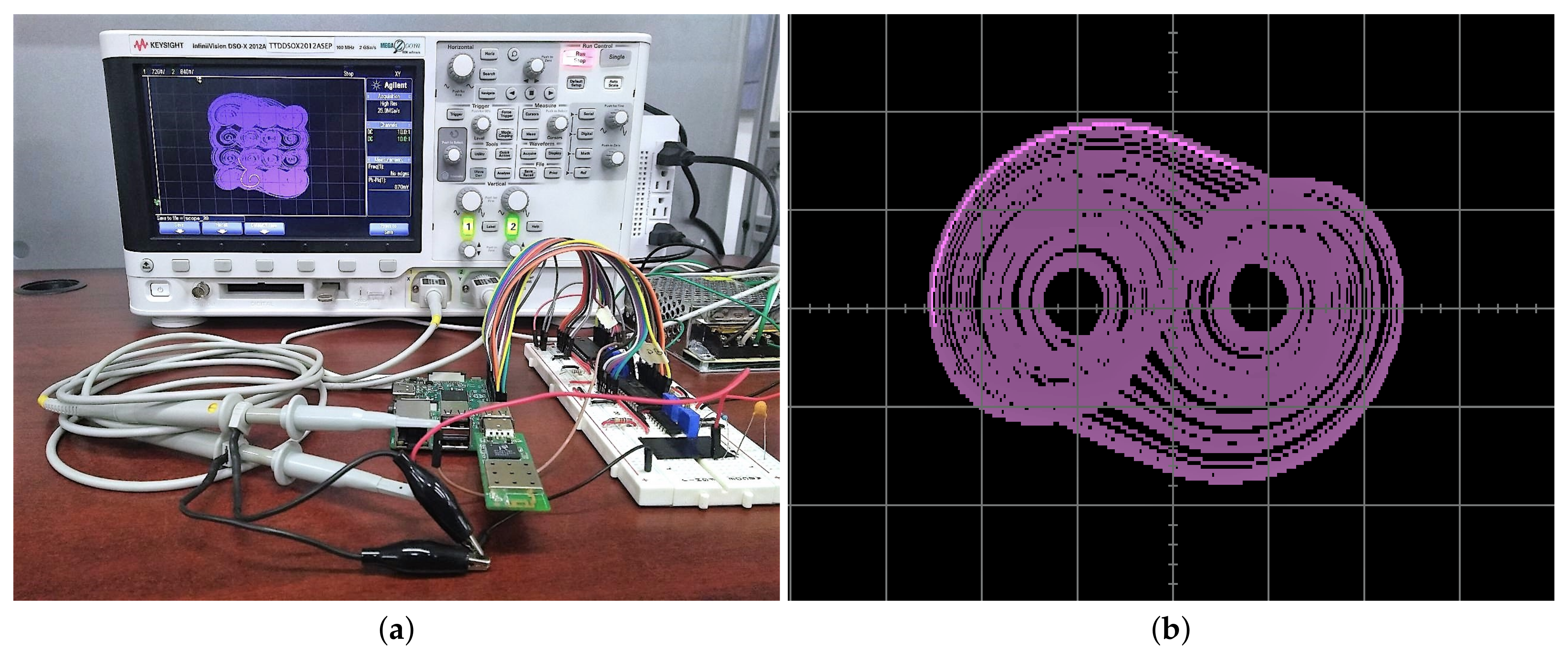
5.2. Embedded Design: PWL-DM Implementation Realized on an ARM Platform
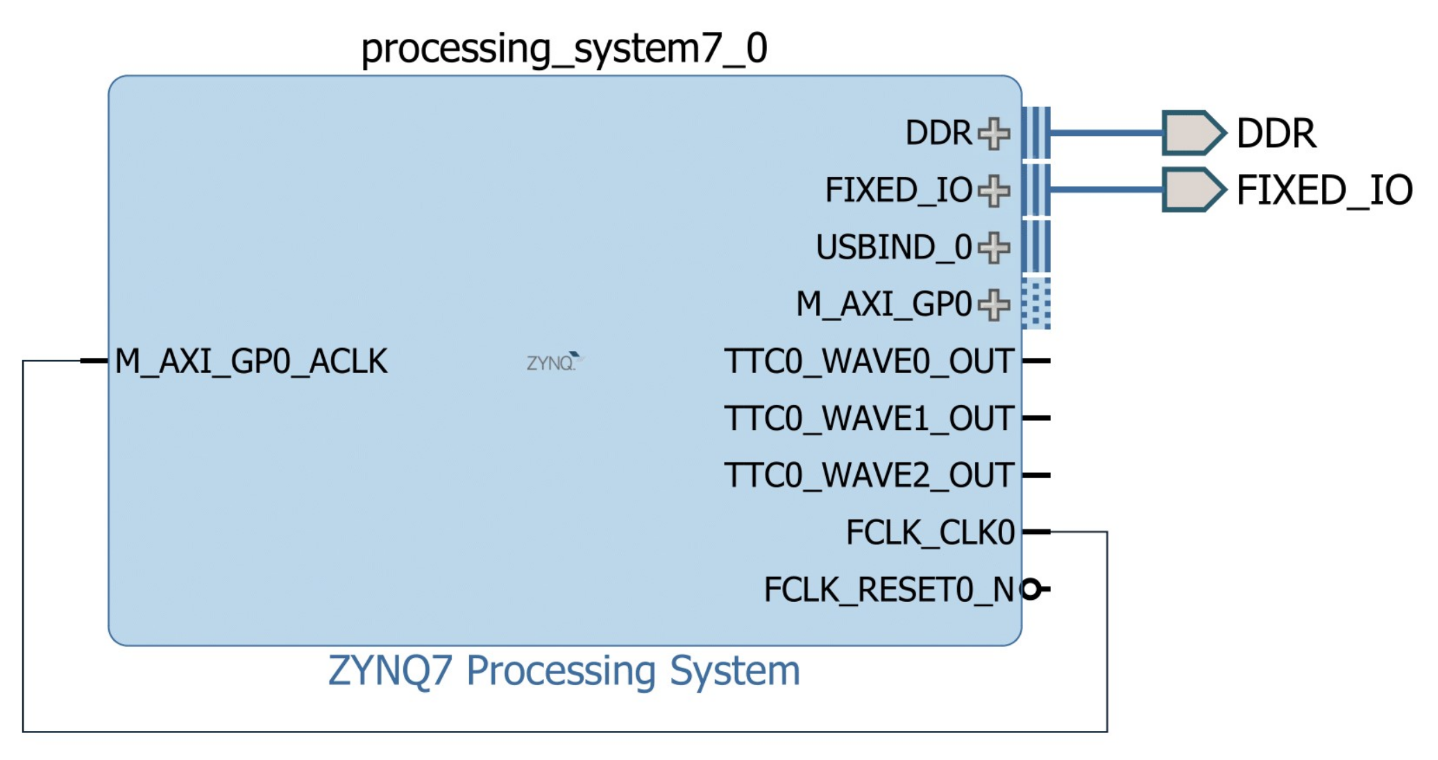
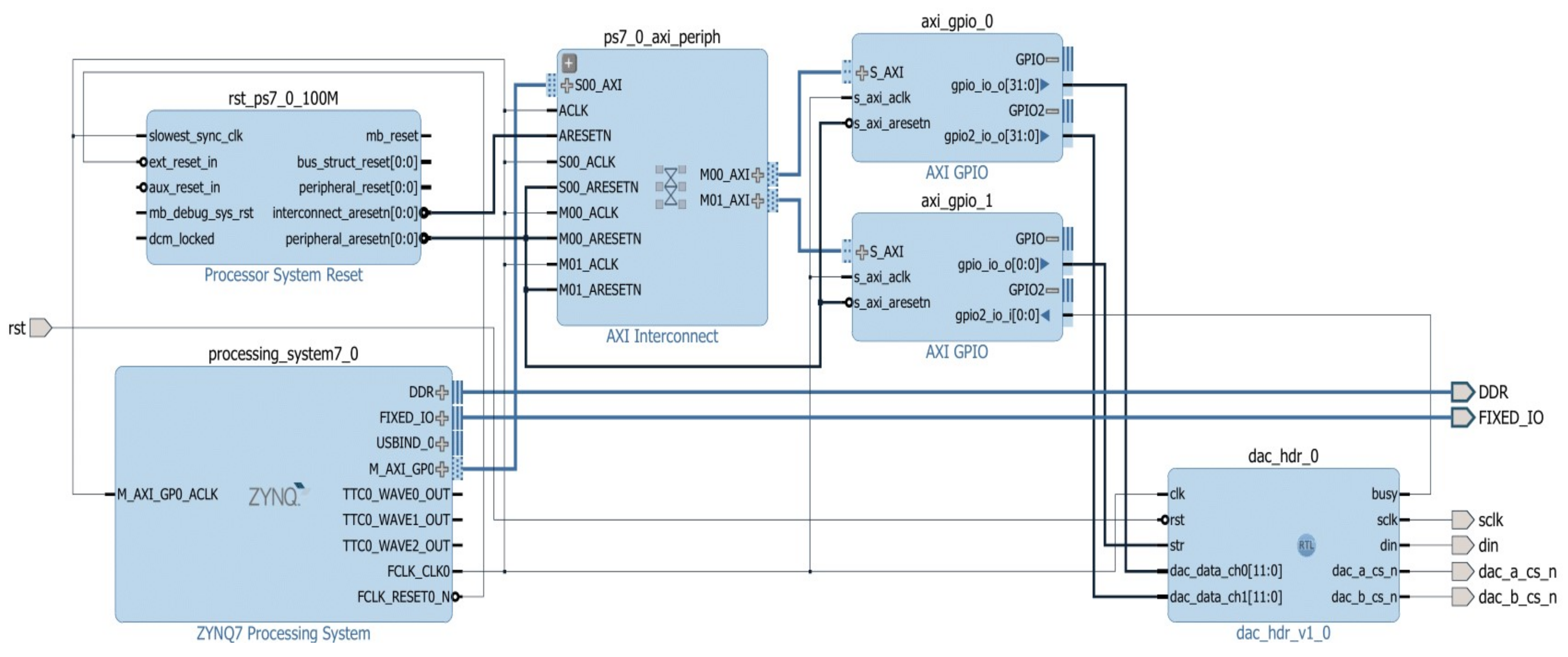
- Device configuration. The ARM-based design illustrated in Figure 13 is elaborated in the Xilinx Vivado Design Suite, version 2016.4. This block contains the ZYNQ7 Processing System IP, which is the software interface around the Processing System (PS) of the Xilinx Zynq-7000 board, currently working at 667 MHz. For including the data converter, a functional interface for communicating the PS with the PL of the Xilinx Zynq-7000 board, operating at 100 MHz, was designed (Figure 14). This interface comprises a Processor System Reset IP, an AXI Interconnect IP, and two AXI GPIO IPs. Later, the dac_hdr_v1_0 is a custom IP for controlling the MCP4922 D/A converter at 20 MHz.
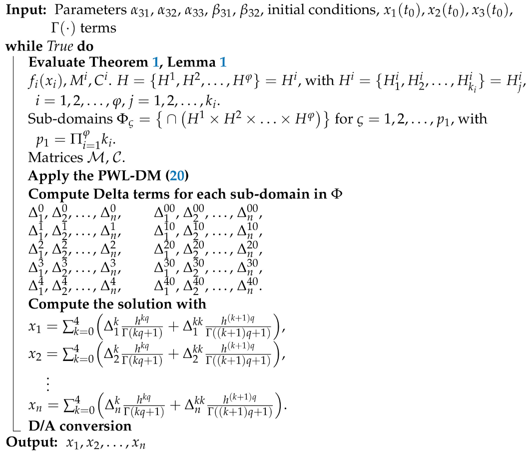
- Calculation Preparation. From now on, the Xilinx Software Development Kit (XSDK), version 2016.4, will be used for the configuration of the PS of the Xilinx Zynq-7000 board in C programming language by using a single-precision (32-bits) floating-point format. The Algorithm 1 shows the pseudo-code for implementing the PWL-DM on an ARM digital platform.
6. Discussion
| Algorithm 1: Pseudocode for implementing the PWL-DM for 2-scrolls (50), 4-scroll (63) and -grid scroll (71) chaotic attractors on an ARM platform. |
 |
7. Conclusions
Author Contributions
Funding
Data Availability Statement
Acknowledgments
Conflicts of Interest
Abbreviations
| Acronym | Description |
| IoT | Internet of Things |
| RNG | Random Number Generator |
| ANN | Artificial Neural Network |
| FDA | Frequency-Domain Approximations |
| GL | Grünwald-Letnikov |
| ABM | Adams-Bashforth-Moulton |
| ADM | Adomian Decomposition Method |
| PWL | Piecewise Linear |
| PWL-DM | Piecewise Linear Decomposition Method |
| ARM | Advanced RISC Machine |
| RISC | Reduced Instruction Set Computer |
| FPGA | Field-Programmable Gate Array |
| CORDIC | coordinate Rotation Digital Computer |
| VHDL | VHSIC Hardware Description Language |
| DSP | Digital Signal Processor |
| PL | Programmable Logic |
| PS | Processing System |
| IP | Intellectual Property |
| RTL | Register Transfer Level |
| MAE | Mean Absolute Error |
| ECO | Expected Convergence Order |
| TR | Trapezoidal rule |
| NGF | Newton–Gregory formula |
| FBDF | Fractional Backward Differentiation Formula |
| Symbol | Description |
| Gamma function | |
| Riemann-Liouville fractional integral operator of order q | |
| Caputo fractional derivative of order q | |
| Finite partition of the phase space | |
| Domains in the phase space partition, | |
| Number of domains in the phase space partition | |
| Subdomains generated by the function | |
| Surfaces specifying the boundaries between consecutive subdomains | |
| Values specifying the boundaries between subdomains in | |
| Piecewise vector in the system definition | |
| Slope and intercept of the piecewise linear functions | |
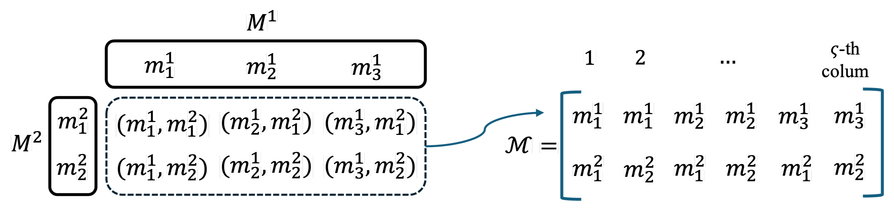
| Matrices composed of the slopes and intercepts of the PWL functions | |
| Number of piecewise linear (PWL) functions | |
| Element of the decomposition series | |
| Initial conditions vector | |
| ADM Coefficients | |
| Number of terms in the approximate solution |
Appendix A

| Sub-Domain | ||
|---|---|---|
| , , , | , , | , , |
| , , | , , | |
| , , | , , | |
| , , | , , | |
| , , | , , | |
| , , | , , | |
| , | , , | , , |
| Sub-Domain | ||
|---|---|---|
| , | , , | , , |
| , | ||
| , | ||
| , | ||
| , | ||
| , | ||
| , | ||
| , | ||
| , , | , , | |
| , , | ||
| , , | ||
| , , | ||
| , , | ||
| , , | , , | |
| Sub-Domain | ||
|---|---|---|
| , , | , , | |
| , , | , , | |
| , , | , , | |
| Sub-Domain | ||
|---|---|---|
| , , | , , | |
| , , | , , | |
| , , | , , | |
References
- Podlubny, I. Fractional differential equations. In Mathematics in Science and Engineering; Elsevier: Amsterdam, The Netherlands, 1999; Volume 198. [Google Scholar]
- Ionescu, C.; Lopes, A.; Copot, D.; Machado, J.T.; Bates, J.H. The role of fractional calculus in modeling biological phenomena: A review. Commun. Nonlinear Sci. Numer. Simul. 2017, 51, 141–159. [Google Scholar] [CrossRef]
- Fernández-Carreón, B.; Munoz-Pacheco, J.; Zambrano-Serrano, E.; Félix-Beltrán, O. Analysis of a Fractional-order Glucose-Insulin Biological System with Time Delay. Chaos Theory Appl. 2022, 4, 10–18. [Google Scholar] [CrossRef]
- Zhou, P.; Ma, J.; Tang, J. Clarify the physical process for fractional dynamical systems. Nonlinear Dyn. 2020, 100, 2353–2364. [Google Scholar] [CrossRef]
- Bǎleanu, D.; Lopes, A.M. (Eds.) Applications in Engineering, Life and Social Sciences, Part A; De Gruyter: Berlin, Germany, 2019. [Google Scholar] [CrossRef]
- Atanackovic, T.M.; Pilipovic, S.; Stankovic, B.; Zorica, D. Fractional Calculus with Applications in Mechanics: Vibrations and Diffusion Processes; John Wiley & Sons: Hoboken, NJ, USA, 2014. [Google Scholar]
- Ghasemi, S.; Tabesh, A.; Askari-Marnani, J. Application of fractional calculus theory to robust controller design for wind turbine generators. IEEE Trans. Energy Convers. 2014, 29, 780–787. [Google Scholar] [CrossRef]
- Tarasov, V.E. On history of mathematical economics: Application of fractional calculus. Mathematics 2019, 7, 509. [Google Scholar] [CrossRef]
- Diethelm, K.; Kiryakova, V.; Luchko, Y.; Machado, J.T.; Tarasov, V.E. Trends, directions for further research, and some open problems of fractional calculus. Nonlinear Dyn. 2022, 107, 3245–3270. [Google Scholar] [CrossRef]
- Sun, K.; He, S.; Wang, H. Solution and Characteristic Analysis of Fractional-Order Chaotic Systems; Springer Nature: Singapore, 2022. [Google Scholar]
- Strogatz, S.H. Nonlinear Dynamics and Chaos: With Applications to Physics, Biology, Chemistry, and Engineering; CRC Press: Boca Raton, FL, USA, 2018. [Google Scholar]
- Ren, L.; Li, S.; Banerjee, S.; Mou, J. A new fractional-order complex chaotic system with extreme multistability and its implementation. Phys. Scr. 2023, 98, 055201. [Google Scholar] [CrossRef]
- Munoz-Pacheco, J.; Zambrano-Serrano, E.; Volos, C.; Jafari, S.; Kengne, J.; Rajagopal, K. A New Fractional-Order Chaotic System with Different Families of Hidden and Self-Excited Attractors. Entropy 2018, 20, 564. [Google Scholar] [CrossRef] [PubMed]
- Xu, S.; Wang, X.; Ye, X. A new fractional-order chaos system of Hopfield neural network and its application in image encryption. Chaos Solitons Fractals 2022, 157, 111889. [Google Scholar] [CrossRef]
- Khan, N.; Muthukumar, P. Transient Chaos, Synchronization and Digital Image Enhancement Technique Based on a Novel 5D Fractional-Order Hyperchaotic Memristive System. Circuits Syst. Signal Process. 2022, 41, 2266–2289. [Google Scholar] [CrossRef]
- Pecora, L.M.; Carroll, T.L. Synchronization in chaotic systems. Phys. Rev. Lett. 1990, 64, 821. [Google Scholar] [CrossRef]
- Ott, E.; Grebogi, C.; Yorke, J.A. Controlling chaos. Phys. Rev. Lett. 1990, 64, 1196. [Google Scholar] [CrossRef] [PubMed]
- Azar, A.T.; Vaidyanathan, S.; Ouannas, A. Fractional Order Control and Synchronization of Chaotic Systems; Springer: Berlin/Heidelberg, Germany, 2017; Volume 688. [Google Scholar]
- Failla, G.; Zingales, M. Advanced materials modelling via fractional calculus: Challenges and perspectives. Philos. Trans. R. Soc. A 2020, 378, 20200050. [Google Scholar] [CrossRef] [PubMed]
- Barros, L.C.d.; Lopes, M.M.; Pedro, F.S.; Esmi, E.; Santos, J.P.C.d.; Sánchez, D.E. The memory effect on fractional calculus: An application in the spread of COVID-19. Comput. Appl. Math. 2021, 40, 1–21. [Google Scholar]
- Abd El-Maksoud, A.J.; Abd El-Kader, A.A.; Hassan, B.G.; Rihan, N.G.; Tolba, M.F.; Said, L.A.; Radwan, A.G.; Abu-Elyazeed, M.F. FPGA implementation of sound encryption system based on fractional-order chaotic systems. Microelectron. J. 2019, 90, 323–335. [Google Scholar] [CrossRef]
- Badr, I.S.; Radwan, A.G.; EL-Rabaie, E.S.M.; Said, L.A.; El-Shafai, W.; El-Banby, G.M.; Abd El-Samie, F.E. Circuit realization and FPGA-based implementation of a fractional-order chaotic system for cancellable face recognition. Multimed. Tools Appl. 2024, 1–26. [Google Scholar] [CrossRef]
- Sayed, W.S.; Roshdy, M.; Said, L.A.; Herencsar, N.; Radwan, A.G. CORDIC-based FPGA realization of a spatially rotating translational fractional-order multi-scroll grid chaotic system. Fractal Fract. 2022, 6, 432. [Google Scholar] [CrossRef]
- Hao, J.; Li, H.; Yan, H.; Mou, J. A new fractional chaotic system and its application in image encryption with DNA mutation. IEEE Access 2021, 9, 52364–52377. [Google Scholar] [CrossRef]
- Yu, F.; Yu, Q.; Chen, H.; Kong, X.; Mokbel, A.A.M.; Cai, S.; Du, S. Dynamic analysis and audio encryption application in IoT of a multi-scroll fractional-order memristive Hopfield neural network. Fractal Fract. 2022, 6, 370. [Google Scholar] [CrossRef]
- Clemente-Lopez, D.; de Jesus Rangel-Magdaleno, J.; Muñoz-Pacheco, J.M. A lightweight chaos-based encryption scheme for IoT healthcare systems. Internet Things 2024, 25, 101032. [Google Scholar] [CrossRef]
- Clemente-López, D.; Munoz-Pacheco, J.M.; de Jesus Rangel-Magdaleno, J. Experimental validation of IoT image encryption scheme based on a 5-D fractional hyperchaotic system and Numba JIT compiler. Internet Things 2024, 25, 101116. [Google Scholar] [CrossRef]
- Yu, F.; Xu, S.; Xiao, X.; Yao, W.; Huang, Y.; Cai, S.; Li, Y. Dynamic analysis and FPGA implementation of a 5D multi-wing fractional-order memristive chaotic system with hidden attractors. Integration 2024, 96, 102129. [Google Scholar] [CrossRef]
- Hu, Z.; Wang, C. Hopfield neural network with multi-scroll attractors and application in image encryption. Multimed. Tools Appl. 2024, 83, 97–117. [Google Scholar] [CrossRef]
- Zhang, S.; Li, C.; Zheng, J.; Wang, X.; Zeng, Z.; Chen, G. Generating any number of diversified hidden attractors via memristor coupling. IEEE Trans. Circuits Syst. I Regul. Pap. 2021, 68, 4945–4956. [Google Scholar] [CrossRef]
- Yan, S.; Wang, Q.; Wang, E.; Sun, X.; Song, Z. Multi-scroll fractional-order chaotic system and finite-time synchronization. Phys. Scr. 2022, 97, 025203. [Google Scholar] [CrossRef]
- Zambrano-Serrano, E.; Munoz-Pacheco, J.M.; Serrano, F.E.; Sánchez-Gaspariano, L.A.; Volos, C. Experimental verification of the multi-scroll chaotic attractors synchronization in PWL arbitrary-order systems using direct coupling and passivity-based control. Integration 2021, 81, 56–70. [Google Scholar] [CrossRef]
- Chen, L.; Pan, W.; Wu, R.; Tenreiro Machado, J.; Lopes, A.M. Design and implementation of grid multi-scroll fractional-order chaotic attractors. Chaos: Interdiscip. J. Nonlinear Sci. 2016, 26, 084303. [Google Scholar] [CrossRef] [PubMed]
- Ahmad, S.; Ullah, A.; Akgül, A. Investigating the complex behaviour of multi-scroll chaotic system with Caputo fractal-fractional operator. Chaos Solitons Fractals 2021, 146, 110900. [Google Scholar] [CrossRef]
- Cui, L.; Luo, W.H.; Ou, Q.L. Analysis and implementation of new fractional-order multi-scroll hidden attractors. Chin. Phys. B 2021, 30, 020501. [Google Scholar] [CrossRef]
- Chen, L.; Pan, W.; Wu, R.; Wang, K.; He, Y. Generation and circuit implementation of fractional-order multi-scroll attractors. Chaos Solitons Fractals 2016, 85, 22–31. [Google Scholar] [CrossRef]
- Diethelm, K.; Garrappa, R.; Stynes, M. Good (and not so good) practices in computational methods for fractional calculus. Mathematics 2020, 8, 324. [Google Scholar] [CrossRef]
- Garrappa, R. Numerical solution of fractional differential equations: A survey and a software tutorial. Mathematics 2018, 6, 16. [Google Scholar] [CrossRef]
- Diethelm, K. The Analysis of Fractional Differential Equations: An Application-Oriented Exposition Using Differential Operators of Caputo Type; Springer Science & Business Media: Berlin/Heidelberg, Germany, 2010. [Google Scholar]
- Clemente-López, D.; Munoz-Pacheco, J.M.; Rangel-Magdaleno, J.d.J. A Review of the Digital Implementation of Continuous-Time Fractional-Order Chaotic Systems Using FPGAs and Embedded Hardware. Arch. Comput. Methods Eng. 2022, 30, 951–983. [Google Scholar] [CrossRef]
- Mohamed, S.M.; Sayed, W.S.; Said, L.A.; Radwan, A.G. Reconfigurable fpga realization of fractional-order chaotic systems. IEEE Access 2021, 9, 89376–89389. [Google Scholar] [CrossRef]
- Tlelo-Cuautle, E.; Pano-Azucena, A.D.; Guillén-Fernández, O.; Silva-Juárez, A. Analog/Digital Implementation of Fractional Order Chaotic Circuits and Applications; Springer: Berlin/Heidelberg, Germany, 2020. [Google Scholar]
- Charef, A.; Sun, H.; Tsao, Y.; Onaral, B. Fractal system as represented by singularity function. IEEE Trans. Autom. Control 1992, 37, 1465–1470. [Google Scholar] [CrossRef]
- Scherer, R.; Kalla, S.L.; Tang, Y.; Huang, J. The Grünwald–Letnikov method for fractional differential equations. Comput. Math. Appl. 2011, 62, 902–917. [Google Scholar] [CrossRef]
- Diethelm, K.; Ford, N.J.; Freed, A.D. A predictor-corrector approach for the numerical solution of fractional differential equations. Nonlinear Dyn. 2002, 29, 3–22. [Google Scholar] [CrossRef]
- Adomian, G. Solving Frontier Problems of Physics: The Decomposition Method; Springer Science & Business Media: Berlin/Heidelberg, Germany, 1994; Volume 1. [Google Scholar]
- Daftardar-Gejji, V.; Jafari, H. Adomian decomposition: A tool for solving a system of fractional differential equations. J. Math. Anal. Appl. 2005, 301, 508–518. [Google Scholar] [CrossRef]
- Tavazoei, M.; Haeri, M. Unreliability of frequency-domain approximation in recognising chaos in fractional-order systems. IET Signal Process. 2007, 1, 171–181. [Google Scholar] [CrossRef]
- Tavazoei, M.S.; Haeri, M.; Bolouki, S.; Siami, M. Stability preservation analysis for frequency-based methods in numerical simulation of fractional order systems. SIAM J. Numer. Anal. 2009, 47, 321–338. [Google Scholar] [CrossRef]
- Brzeziński, D.W. Fractional Order Derivative and Integral Computation with a Small Number of Discrete Input Values Using Grünwald–Letnikov Formula. Int. J. Comput. Methods 2020, 17, 1940006. [Google Scholar] [CrossRef]
- Wu, G.C.; Luo, M.; Huang, L.L.; Banerjee, S. Short memory fractional differential equations for new memristor and neural network design. Nonlinear Dyn. 2020, 100, 3611–3623. [Google Scholar] [CrossRef]
- Gu, C.Y.; Wu, G.C.; Shiri, B. An inverse problem approach to determine possible memory length of fractional differential equations. Fract. Calc. Appl. Anal. 2021, 24, 1919–1936. [Google Scholar] [CrossRef]
- Deng, W. Short memory principle and a predictor–corrector approach for fractional differential equations. J. Comput. Appl. Math. 2007, 206, 174–188. [Google Scholar] [CrossRef]
- Clemente-López, D.; Muñoz-Pacheco, J.M.; Félix-Beltrán, O.G.; Volos, C. Efficient Computation of the Grünwald-Letnikov Method for ARM-Based Implementations of Fractional-Order Chaotic Systems. In Proceedings of the 2019 8th International Conference on Modern Circuits and Systems Technologies (MOCAST), Thessaloniki, Greece, 13–15 May 2019; pp. 1–4. [Google Scholar]
- Tolba, M.F.; Saleh, H.; Mohammad, B.; Al-Qutayri, M.; Elwakil, A.S.; Radwan, A.G. Enhanced FPGA realization of the fractional-order derivative and application to a variable-order chaotic system. Nonlinear Dyn. 2020, 99, 3143–3154. [Google Scholar] [CrossRef]
- MacDonald, C.L.; Bhattacharya, N.; Sprouse, B.P. Efficient computation of the Grünwald-Letnikov fractional diffusion derivative using adaptive time step memory. J. Comput. Phys. 2015, 297, 221–236. [Google Scholar] [CrossRef]
- Tolba, M.F.; AbdelAty, A.M.; Soliman, N.S.; Said, L.A.; Madian, A.H.; Azar, A.T.; Radwan, A.G. FPGA implementation of two fractional order chaotic systems. AEU-Int. J. Electron. Commun. 2017, 78, 162–172. [Google Scholar] [CrossRef]
- He, S.; Wang, H.; Sun, K. Solutions and memory effect of fractional-order chaotic system: A review. Chin. Phys. B 2022, 31, 060501. [Google Scholar] [CrossRef]
- Wazwaz, A.M. A new algorithm for calculating Adomian polynomials for nonlinear operator. Appl. Math. Comput. 2000, 111, 33–51. [Google Scholar] [CrossRef]
- Cafagna, D.; Grassi, G. Fractional-order Chua’s circuit: Time-domain analysis, bifurcation, chaotic behavior and test for chaos. Int. J. Bifurc. Chaos 2008, 18, 615–639. [Google Scholar] [CrossRef]
- Guo, P. The adomian decomposition method for a type of fractional differential equations. J. Appl. Math. Phys. 2019, 7, 2459–2466. [Google Scholar] [CrossRef]
- Li, G.; Zhang, X.; Yang, H. Numerical analysis, circuit simulation, and control synchronization of fractional-order unified chaotic system. Mathematics 2019, 7, 1077. [Google Scholar] [CrossRef]
- Wang, H.; Sun, K.; He, S. Characteristic analysis and DSP realization of fractional-order simplified Lorenz system based on Adomian decomposition method. Int. J. Bifurc. Chaos 2015, 25, 1550085. [Google Scholar] [CrossRef]
- Gu, S.; He, S.; Wang, H.; Du, B. Analysis of three types of initial offset-boosting behavior for a new fractional-order dynamical system. Chaos Solitons Fractals 2021, 143, 110613. [Google Scholar] [CrossRef]
- Yang, F.; Wang, X. Dynamic characteristic of a new fractional-order chaotic system based on the Hopfield Neural Network and its digital circuit implementation. Phys. Scr. 2021, 96, 035218. [Google Scholar] [CrossRef]
- Liu, T.; Yan, H.; Banerjee, S.; Mou, J. A fractional-order chaotic system with hidden attractor and self-excited attractor and its DSP implementation. Chaos Solitons Fractals 2021, 145, 110791. [Google Scholar] [CrossRef]
- Rajagopal, K.; Kingni, S.T.; Khalaf, A.J.M.; Shekofteh, Y.; Nazarimehr, F. Coexistence of attractors in a simple chaotic oscillator with fractional-order-memristor component: Analysis, FPGA implementation, chaos control and synchronization. Eur. Phys. J. Spec. Top. 2019, 228, 2035–2051. [Google Scholar] [CrossRef]
- Xu, J.; Mou, J.; Liu, J.; Hao, J. The image compression–encryption algorithm based on the compression sensing and fractional-order chaotic system. Vis. Comput. 2021, 38, 1509–1526. [Google Scholar] [CrossRef]
- Wang, H.; Sun, K.; He, S. Dynamic analysis and implementation of a digital signal processor of a fractional-order Lorenz-Stenflo system based on the Adomian decomposition method. Phys. Scr. 2014, 90, 015206. [Google Scholar] [CrossRef]
- He, S.; Sun, K.; Wang, H. Dynamics of the fractional-order Lorenz system based on Adomian decomposition method and its DSP implementation. IEEE/CAA J. Autom. Sin. 2016, 11, 1298–1300. [Google Scholar] [CrossRef]
- Fu, H.; Lei, T. Adomian Decomposition, Dynamic Analysis and Circuit Implementation of a 5D Fractional-Order Hyperchaotic System. Symmetry 2022, 14, 484. [Google Scholar] [CrossRef]
- Rajagopal, K.; Karthikeyan, A.; Srinivasan, A. Dynamical analysis and FPGA implementation of a chaotic oscillator with fractional-order memristor components. Nonlinear Dyn. 2018, 91, 1491–1512. [Google Scholar] [CrossRef]
- Jafari, H.; Daftardar-Gejji, V. Solving a system of nonlinear fractional differential equations using Adomian descomposition. J. Comput. Appl. Math. 2006, 196, 644–651. [Google Scholar] [CrossRef]
- Zaouagui, I.; Badredine, T. New Adomian’s Polynomials Formulas for the Non-linear and Non-autonomous Ordinary Differential Equations. J. Appl. Comput. Math 2017, 6, 373. [Google Scholar]
- Mahdi, S.H.; Jassim, H.K. A new technique of using adomian decomposition method for fractional order nonlinear differential equations. Conf. Proc. 2023, 2414, 040075. [Google Scholar]
- Duan, J.S.; Chaolu, T.; Rach, R.; Lu, L. The Adomian decomposition method with convergence acceleration techniques for nonlinear fractional differential equations. Comput. Math. Appl. 2013, 66, 728–736. [Google Scholar] [CrossRef]
- Razali, N.I.; Chowdhury, M.; Asrar, W. The multistage adomian decomposition method for solving chaotic lü system. Middle-East J. Sci. Res. 2013, 13, 43–49. [Google Scholar]
- Song, L.; Wang, W. A new improved Adomian decomposition method and its application to fractional differential equations. Appl. Math. Model. 2013, 37, 1590–1598. [Google Scholar] [CrossRef]
- Lü, J.; Chen, G. Generating multiscroll chaotic attractors: Theories, methods and applications. Int. J. Bifurc. Chaos 2006, 16, 775–858. [Google Scholar] [CrossRef]
- Deng, W.; Lü, J. Design of multidirectional multiscroll chaotic attractors based on fractional differential systems via switching control. Chaos Interdiscip. J. Nonlinear Sci. 2006, 16, 043120. [Google Scholar] [CrossRef]
- Echenausía-Monroy, J.; Gilardi-Velázquez, H.; Wang, N.; Jaimes-Reátegui, R.; García-López, J.; Huerta-Cuellar, G. Multistability route in a PWL multi-scroll system through fractional-order derivatives. Chaos Solitons Fractals 2022, 161, 112355. [Google Scholar] [CrossRef]
- Altun, K. Multi-Scroll Attractors with Hyperchaotic Behavior Using Fractional-Order Systems. J. Circuits Syst. Comput. 2022, 31, 2250085. [Google Scholar] [CrossRef]
- Pan, W.; Chen, L.; Zhang, W. Design of a class of fractional-order hyperchaotic multidirectional multi-scroll attractors. Math. Methods Appl. Sci. 2021, 44, 2416–2430. [Google Scholar] [CrossRef]
- Liu, S.; Wei, Y.; Liu, J.; Chen, S.; Zhang, G. Multi-scroll chaotic system model and its cryptographic application. Int. J. Bifurc. Chaos 2020, 30, 2050186. [Google Scholar] [CrossRef]
- De la Fraga, L.G.; Mancillas-López, C.; Tlelo-Cuautle, E. Designing an authenticated Hash function with a 2D chaotic map. Nonlinear Dyn. 2021, 104, 4569–4580. [Google Scholar] [CrossRef]
- Azzaz, M.S.; Tanougast, C.; Maali, A.; Benssalah, M. Hardware implementation of multi-scroll chaos based architecture for securing biometric templates. In Proceedings of the 2018 International Conference on Smart Communications in Network Technologies (SaCoNeT), El Oued, Algeria, 27–31 October 2018; pp. 227–231. [Google Scholar]
- Storace, M.; De Feo, O. PWL approximation of nonlinear dynamical systems, part I: Structural stability. J. Phys. Conf. Ser. 2005, 22, 208. [Google Scholar] [CrossRef]
- Sun, H.; Cao, H. Chaos control and synchronization of a modified chaotic system. Chaos Solitons Fractals 2008, 37, 1442–1455. [Google Scholar] [CrossRef]
- Petrzela, J. On the piecewise-linear approximation of the polynomial chaotic dynamics. In Proceedings of the 2011 34th International Conference on Telecommunications and Signal Processing (TSP), Budapest, Hungary, 18–20 August 2011; pp. 319–323. [Google Scholar]
- Gorenflo, R.; Mainardi, F. Fractional calculus. In Fractals and Fractional Calculus in Continuum Mechanics; Springer: Berlin/Heidelberg, Germany, 1997; pp. 223–276. [Google Scholar]
- Ross, B. A brief history and exposition of the fundamental theory of fractional calculus. In Fractional Calculus and Its Applications; Springer: Berlin/Heidelberg, Germany, 1975; pp. 1–36. [Google Scholar]
- Cafagna, D.; Grassi, G. Adomian descomposition method as a tool for numerical studying multi-scroll hyperchaotic attractors. In Proceedings of the International Symposium on Nonlinear Theory and Its Applications (NOLTA2005), Bruges, Belgium, 18–21 October 2005. [Google Scholar]
- Moghaddam, B.P.; Machado, J.A.T. Extended algorithms for approximating variable order fractional derivatives with applications. J. Sci. Comput. 2017, 71, 1351–1374. [Google Scholar] [CrossRef]
- Tavazoei, M.S.; Haeri, M. A necessary condition for double scroll attractor existence in fractional-order systems. Phys. Lett. A 2007, 367, 102–113. [Google Scholar] [CrossRef]
- Garrappa, R. Trapezoidal methods for fractional differential equations: Theoretical and computational aspects. Math. Comput. Simul. 2015, 110, 96–112. [Google Scholar] [CrossRef]
- Qiu, M.; Yu, S.; Wen, Y.; Lü, J.; He, J.; Lin, Z. Design and FPGA implementation of a universal chaotic signal generator based on the Verilog HDL fixed-point algorithm and state machine control. Int. J. Bifurc. Chaos 2017, 27, 1750040. [Google Scholar] [CrossRef]
- Petráš, I. Fractional-Order Nonlinear Systems: Modeling, Analysis and Simulation; Springer Science & Business Media: Berlin/Heidelberg, Germany, 2011. [Google Scholar]
- Pano-Azucena, A.D.; Tlelo-Cuautle, E.; Muñoz-Pacheco, J.M.; de la Fraga, L.G. FPGA-based implementation of different families of fractional-order chaotic oscillators applying Grünwald–Letnikov method. Commun. Nonlinear Sci. Numer. Simul. 2019, 72, 516–527. [Google Scholar] [CrossRef]


| Fractional Order | Step Size | MAE | ECO |
|---|---|---|---|
| 2−Terms |  | 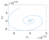 | 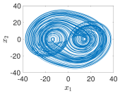 | 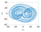 |
| 3−Terms | 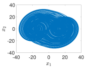 | 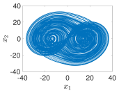 |  | 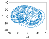 |
| 4−Terms |  | 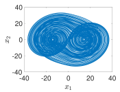 |  | 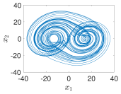 |
| 5−Terms |  | 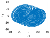 | 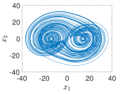 | 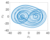 |
| FPGA Implementation | ||||
|---|---|---|---|---|
| Hardware | Available | 2-scrolls | 4-scrolls | -Grid Scrolls |
| LUT | 53,200 | 1469 (2.75%) | 1588 (2.98%) | 2330 (4.38%) |
| FF | 106,400 | 1155 (1.08%) | 1123 (1.06%) | 1170 (1.10%) |
| DSP | 220 | 4 (1.82%) | 4 (1.82%) | 12 (5.45%) |
| BRAM | 140 | 0 (0%) | 0 (0%) | 0 (0%) |
| IO | 200 | 98 (49.0%) | 98 (49.0%) | 98 (49.0%) |
| BUFG | 32 | 1 (3.13%) | 1 (3.13%) | 1 (3.13%) |
| ARM implementation | ||||
| Hardware | Available | 2-scrolls, 4-scrolls, -grid scrolls | ||
| LUT | 53,200 | 676 (1.27%) | ||
| FF | 106,400 | 62 (0.36%) | ||
| DSP | 220 | 879 (0.83%) | ||
| IO | 200 | 5 (2.50%) | ||
| BUFG | 32 | 1 (3.13%) | ||
| FPGA Implementation | Clock Frequency (MHz) | Throughput (Gbit/s) |
|---|---|---|
| 2-scrolls | 110.238 | 3.527 |
| 4-scrolls | 103.627 | 3.316 |
| -grid scrolls | 91.106 | 2.915 |
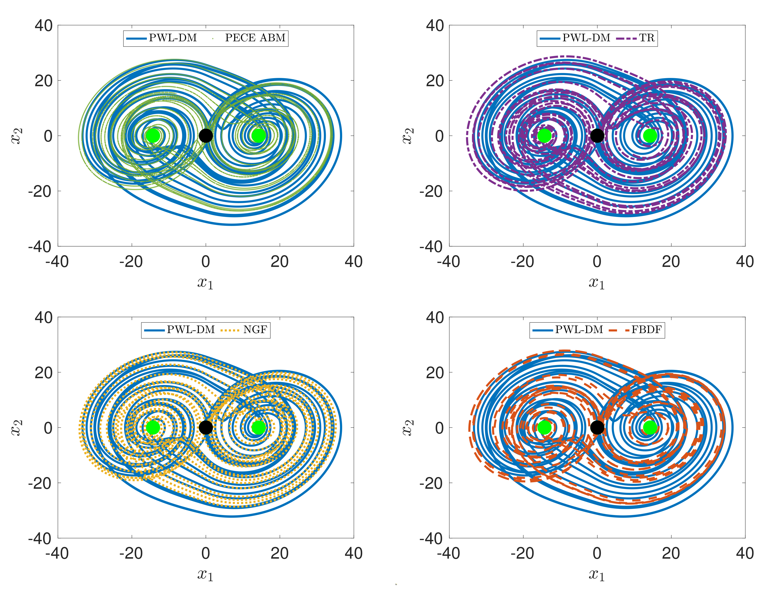
| Algorithm | Integration Step-Size, h | Simulation Time | No. of Iterations | Computation Time |
|---|---|---|---|---|
| ABM [45] | 0.01 | 2000 s | 133,333 | 2809.19 s |
| Short-memory GL [54,97], p. 19 | 0.01 | 2000 s | 133,333 | 12.91 s |
| PWL-DM (This work) | 0.01 | 2000 s | 133,333 | 0.88 s |
| Resource | Available | PWL-DM (This Work) | Short-Memory GL (Design Guidelines in Ref. [40]) |
|---|---|---|---|
| LUT | 53,200 | 1469 (2.75%) | 3197 (6.01%) |
| FF | 106,400 | 1155 (1.08%) | 838 (0.79%) |
| DSP | 220 | 4 (1.82%) | 20 (9.09%) |
| BRAM | 140 | 0 (0%) | 1.5 (1.07%) |
| IO | 200 | 98 (49%) | 98 (49%) |
| BUFG | 32 | 1 (3.13%) | 1 (3.13%) |
| Item | Tang System (Short-Memory GL) | Özoguz System (Short-Memory GL) | Yalcin System (Short-Memory GL) | Lü System in Equation (27) (Short-Memory GL) | V-Shape System (Short-Memory GL) | Lü System in Equation (27) (PWL-DM) |
|---|---|---|---|---|---|---|
| Nonlinearity | PWL function | PWL function | PWL function | PWL function | PWL function | PWL function |
| Attractor | 1D multi-scroll | 1D multi-scroll | 1D multi-scroll | 1D multi-scroll | 1D multi-scroll | 1D multi-scroll |
| LUT | 3339 | 3856 | 2125 | – | – | 1588 |
| FF | 1763 | 2597 | 1932 | – | – | 1123 |
| DSP | 134 | 194 | 132 | – | 59 | 4 |
| BRAM | 0 | 0 | 0 | 3 | 0 | 0 |
| Max. Clock (MHz) | 67.378 | 42.052 | 94.941 | 84.34 | 73.049 | 103.627 |
| Throughput (Gb/s) | 2.156 | 1.345 | 3.038 | 2.69 | 2.921 | 3.316 |
| FPGA chip & Design suite | Artix-7 ISE 14.5 | Artix-7 ISE 14.5 | Artix-7 ISE 14.5 | Cyclone IV-GX Quartus | Virtex-5 ISE 14.5 | Artix-7 Vivado 2016.4 |
| Ref. | [21] | [21] | [21] | [98] | [57] | This work |
Disclaimer/Publisher’s Note: The statements, opinions and data contained in all publications are solely those of the individual author(s) and contributor(s) and not of MDPI and/or the editor(s). MDPI and/or the editor(s) disclaim responsibility for any injury to people or property resulting from any ideas, methods, instructions or products referred to in the content. |
© 2024 by the authors. Licensee MDPI, Basel, Switzerland. This article is an open access article distributed under the terms and conditions of the Creative Commons Attribution (CC BY) license (https://creativecommons.org/licenses/by/4.0/).
Share and Cite
Clemente-López, D.; Munoz-Pacheco, J.M.; Zambrano-Serrano, E.; Félix Beltrán, O.G.; Rangel-Magdaleno, J.d.J. A Piecewise Linear Approach for Implementing Fractional-Order Multi-Scroll Chaotic Systems on ARMs and FPGAs. Fractal Fract. 2024, 8, 389. https://doi.org/10.3390/fractalfract8070389
Clemente-López D, Munoz-Pacheco JM, Zambrano-Serrano E, Félix Beltrán OG, Rangel-Magdaleno JdJ. A Piecewise Linear Approach for Implementing Fractional-Order Multi-Scroll Chaotic Systems on ARMs and FPGAs. Fractal and Fractional. 2024; 8(7):389. https://doi.org/10.3390/fractalfract8070389
Chicago/Turabian StyleClemente-López, Daniel, Jesus M. Munoz-Pacheco, Ernesto Zambrano-Serrano, Olga G. Félix Beltrán, and Jose de Jesus Rangel-Magdaleno. 2024. "A Piecewise Linear Approach for Implementing Fractional-Order Multi-Scroll Chaotic Systems on ARMs and FPGAs" Fractal and Fractional 8, no. 7: 389. https://doi.org/10.3390/fractalfract8070389
APA StyleClemente-López, D., Munoz-Pacheco, J. M., Zambrano-Serrano, E., Félix Beltrán, O. G., & Rangel-Magdaleno, J. d. J. (2024). A Piecewise Linear Approach for Implementing Fractional-Order Multi-Scroll Chaotic Systems on ARMs and FPGAs. Fractal and Fractional, 8(7), 389. https://doi.org/10.3390/fractalfract8070389