Abstract
In this study, we focus on the stability analysis of the RLC model by employing differential equations with Hadamard fractional derivatives. We prove the existence and uniqueness of solutions using Banach’s contraction principle and Schaefer’s fixed point theorem. To facilitate our key conclusions, we convert the problem into an equivalent integro-differential equation. Additionally, we explore several versions of Ulam’s stability findings. Two numerical examples are provided to illustrate the applications of our main results. We also observe that modifications to the Hadamard fractional derivative lead to asymmetric outcomes. The study concludes with an applied example demonstrating the existence results derived from Schaefer’s fixed point theorem. These findings represent novel contributions to the literature on this topic, significantly advancing our understanding.
1. Introduction
Fractional calculus extends traditional differential and integral calculus by introducing the concept of non-integer orders. Utilizing fractional derivatives such as the Caputo–Hadamard and Riemann–Liouville derivatives, this discipline provides a robust framework for modeling systems with nonlocal or memory-dependent behaviors [1,2,3]. Fractional differential equations, a key component of fractional calculus, represent a vibrant area of research with significant implications across various disciplines. Researchers have extensively explored the applications of these equations in fields such as physics, biology, and finance [4,5,6,7,8,9,10]. These equations have been instrumental in systematically examining and understanding phenomena like anomalous diffusion, fractal characteristics, and long-range interactions. The study of fractional calculus has revolutionized mathematical modeling and analysis, offering deeper insights into the complexities of dynamical processes that conventional calculus methods cannot adequately address. The literature reflects a growing body of research focused on leveraging the power of fractional differential equations to tackle real-world challenges and phenomena across diverse domains see in [11,12,13,14].
In recent years, the study of Hadamard fractional derivatives has emerged as a focal point in mathematical research. The Hadamard fractional derivative offers advantages over other fractional derivatives due to its capability to handle non-differentiable functions and its suitability for various applications [15,16,17,18,19,20,21,22,23]. This derivative has found applications in modeling complex systems where memory effects or nonlocal interactions play a crucial role. Moreover, its application in differential equations has expanded the scope of mathematical modeling, enabling more accurate descriptions of real-world phenomena. Researchers have employed Hadamard fractional derivatives in diverse contexts, including physics, engineering, and stochastic processes. For example, Ref. [24] discusses the implications of Hadamard fractional differential equations with varying coefficients, emphasizing their relevance in probabilistic applications. This work highlights the flexibility of Hadamard derivatives in capturing complex dynamics where coefficients vary over time, enhancing the modeling capabilities in probabilistic contexts. Ref. [25] explores numerical methods for Caputo–Hadamard fractional derivatives (HFD), demonstrating their effectiveness in the long-term integration of fractional differential systems. Their study underscores the practical utility of these derivatives in numerical simulations, providing robust techniques for handling fractional differential equations with varying initial conditions and system parameters.
Fixed point theorems, such as Banach’s contraction mapping principle and Schaefer’s fixed point theorem, are pivotal in establishing the existence and uniqueness of solutions in mathematical analysis. Banach’s theorem asserts that in a complete metric space, a contraction mapping has a unique fixed point, essential for proving solutions to equations
. Schaefer’s theorem extends these principles to more general settings, allowing for the study of mappings defined on Banach spaces and providing versatile tools for stability analysis and solution validation in differential equations with HFDs [26,27,28].
The study of fractional stochastic differential equations has advanced mathematical modeling and analysis, offering valuable insights into real-world phenomena. Research on stability analysis is widely available across different platforms across in a stability analysis, such as physics and engineering, highlights the promising potential of differential equations in unraveling and forecasting complex system dynamics [29,30,31]. Recently, the stability analysis of systems described by differential equations involving Hadamard fractional derivatives has also attracted considerable research interest. Stability is a fundamental property in understanding the behavior of dynamical systems under perturbations. Techniques such as Banach’s contraction principle and Schaefer’s fixed point theorem have been applied to establish the existence and uniqueness of solutions in this context. Ref. [30] focused on Lyapunov stability analysis, and Ref. [31] explored averaging techniques for stability assessment. Ulam–Hyers (UH) stability theory, named after Stanislaw Ulam and Donald Hyers, deals with the stability of functional equations and has applications in various branches of mathematics. This theory provides a framework for investigating the robustness of solutions to perturbations, offering valuable insights into the stability properties of mathematical models in diverse contexts. Moreover, the Ulam–Hyers stability theory provides a robust framework for assessing the stability of solutions to functional equations, including those involving fractional derivatives [32].
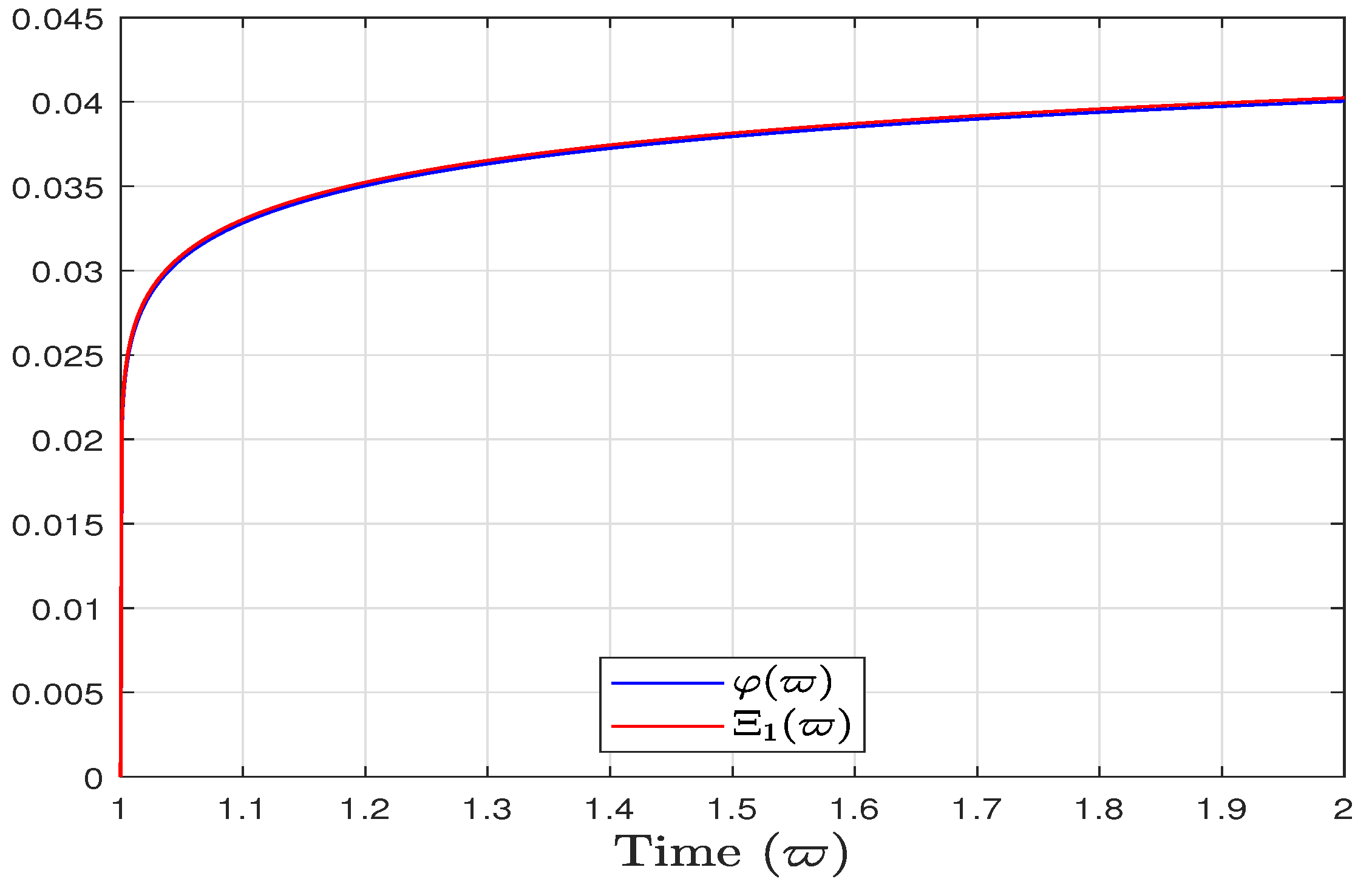
The differential equations are extensively applied in scientific and engineering fields, particularly in circuit analysis. Based on Kirchhoff’s second law, the equations for the RLC circuit demonstrate the principle of energy conservation, which states that the total voltage drop around a closed loop must equal the applied voltage
. This relationship can be represented mathematically as follows:
An RLC circuit is a fundamental component in electrical engineering, comprising a resistor R, inductor L, and capacitor C connected in series with a voltage source, such as a battery or generator, providing a time-dependent voltage
. The resistor dissipates energy as heat, the inductor stores energy in its magnetic field, and the capacitor stores energy in its electric field. The behavior of the circuit can be analyzed in different frequency domains, which is crucial for applications in signal processing, communications, and power distribution. By solving the differential equation, one can determine the current
and voltage across each component over time, leading to insights into the circuit’s transient and steady-state response. This configuration, illustrated in Figure 1, embodies the essence of complex electrical networks. With its resistor offering resistance R ohms, inductor providing inductance L henries, and capacitor furnishing capacitance C farads, the RLC circuit forms a fundamental structure for understanding electrical dynamics.

Figure 1.
Block diagram for the RLC series circuit.
The authors in [33] recently explored the fractional-order (FO) RLC derivative using three numerical methodologies. This research sheds light on the intricate behavior of FO systems within the RLC framework.
Motivated by the aforementioned research, our study investigates the Hadamard FO RLC circuit integro-differential equation (IDE), coupled with nonlocal boundary constraints. Our goal is to prove existence and uniqueness of solutions by applying fixed point theorems of Schaefer and Banach. Additionally, our investigation extends to Ulam stability analysis, offering insights into the system’s robustness. Drawing upon the Hyers–Ulam stability theory and the Ulam–Hyers–Rassias (UHR) stability framework, we explore the stability characteristics of the system.
The relationship between stability and symmetry in differential equations has long been a topic of interest, explored by many researchers across various fields. For instance, it has been examined in contexts like irreversible thermodynamics [34] and time-reversal symmetry in nonequilibrium statistical mechanics [35]. Additionally, the interaction between symmetries and stability plays a crucial role in understanding and controlling nonlinear dynamical systems and networks [36].
As such, this issue also becomes pertinent in differential equations involving fractional derivatives. The stability of solutions is recognized as a fundamental property of functional differential equations. In this paper, we investigate stability in the Ulam–Hyers–Rassias sense of Equation (4), providing theoretical insights supported by an illustrative example.
Through rigorous analysis and numerical simulations, we validate our findings, ensuring the reliability and applicability of the obtained results.
The main contribution of this work can be given as follows: 1. In this paper, we have presented a unique application of the fractional Hadamard derivative in the stability analysis of the RLC model, which is not frequently studied in the existing literature. 2. By applying Banach’s contraction principle and Schaefer’s fixed point theorem, new results on the existence and uniqueness of solutions for fractional differential equations are established, which is a challenging mathematical approach. And 3. The investigation of different versions of Ulam’s stability provides new insights and extends the current understanding of stability in fractional differential Equation (4). The theoretical results are validated by numerical examples.
2. Preliminaries and Problem Statement
In this section, we review some fundamental definitions, properties, theorems, and lemmas that are essential for the subsequent sections of this paper. These foundational concepts will provide the necessary framework for our analysis and help in understanding the more advanced discussions that follow. By familiarizing ourselves with these basics, we can better appreciate the complexities of the topics addressed later in the paper. In Table 1, we have provided the definition of a Banach space along with the norm condition.

Table 1.
Banach space and Norm.
Table 1.
Banach space and Norm.
| Symbol | Definition |
|---|---|
| Space of continuous functions from to | |
| Norm: | |
| Product | |
| Banach space with Norm: |
This formulation establishes a foundational framework for our subsequent analysis, providing a mathematical basis for the exploration of the properties and behavior of functions within
. The Banach space structure of
enables us to employ powerful analytical tools to investigate the solutions and dynamics of the FO RLC circuit IDEs. Through this groundwork, we pave the way for accurate mathematical analysis and insightful interpretations in our study.
Definition 1
([37]). The Caputo derivatives of order ω for the function
is defined as:
Problem Formulation
Consider the integro-differential equation for the Hadamard fractional-order RLC circuit: along with its nonlocal boundary conditions.
where
is the HFD of order
.
For the system described by Equation (5), we can define the nonlocal boundary condition as follows:
where,
is the Riemann–Liouville fractional integral of order
.
The structure of the RLC model is as follows:
and
We establish the solutions of Equation (5) by applying Banach’s and Schaefer’s fixed point theorems. These powerful mathematical tools provide robust guarantees regarding the existence and uniqueness of solutions, ensuring the validity of our analysis. Through the application of these theorems, we demonstrate the fundamental properties of solutions to Equation (5), laying a solid mathematical foundation for further investigation and analysis.
Definition 2
([38]). The Hadamard fractional (HF) integral of order
for a continuous function
is given by
where
.
Definition 3
([38]). The HF derivative of order
for a function
is defined by
where
is the gamma function.
Lemma 1
([38]). If
and
, then
In particular, for
, we have
Lemma 2.
For
, it is a solution of the BVPs,
which satisfies the following equation:
suppressive case
where
.
Proof.
According to the results in [37], the solution to the HDE described in (11) can be formulated as follows:
Utilizing the provided BCs, it follows that
. Consequently, we derive:
from our condition, and by using BCs (11), one has
from which we obtain
Assumption 1.
The function
is completely continuous, and there exists a function
satisfying:
Assumption 2.
The function
exhibits continuity, with positive constants
and
satisfying:
Assumption 3.
The function
maintains continuity, with the existence of a positive constant
satisfying:
3. Main Results
Here, we establish certain assumptions for the subsequent analysis.
Considering Lemma 2, we can introduce
as follows:
Suitable for computation, we represent:
Theorem 1.
If Assumption 1 holds true, then Equation (5) has at least one solution defined on
.
Proof.
To establish the existence of a fixed point for
on
, we will employ Schaefer’s fixed point theorem. Notably, the continuity of
ensures the continuity of
on
. This fundamental continuity property underscores the applicability of Schaefer’s theorem in our analysis, providing a solid foundation for our proof.
Next, we aim to demonstrate that
. Consider
, and let
for each
. Then, for each
, we have:
Step 1: Continuity of
.
To establish the continuity of
, we consider a sequence
converging to
in
. For any
, we examine the behavior of
under this convergence. By the properties of
, we aim to show that
converges to
as n tends to infinity. This continuity property is crucial for subsequent analysis involving
.
Given the continuity of the function
, we can conclude that
Hence, we establish the continuity of the operator
.
Now, let us proceed to Step 2: Demonstrating that
is bounded. This step is crucial in our analysis, as it ensures the boundedness of the image of bounded sets under the operator
, a prerequisite for the application of Schaefer’s fixed point theorem. Through rigorous analysis, we aim to provide a clear understanding of how
transforms bounded sets within
, underscoring its significance in our proof.
For each
and for any
, it follows that:
Thus,
.
Step 3: Establishing the equi-continuity of
. This step is essential, as it confirms that the images of bounded sets under
exhibit uniform continuity. By demonstrating the equi-continuity of
, we strengthen our argument for the applicability of Schaefer’s fixed point theorem. Through meticulous analysis, we aim to elucidate the uniform behavior of
across bounded sets, further validating its role in our proof.
For
, and
, we obtain
As
approaches
, the right-hand side of the inequality converges to zero. This observation leads to the conclusion that
is completely continuous, given its behavior under varying parameters. This property is essential for ensuring the stability and convergence of subsequent analyses reliant on
.
Step 4: Establish a priori bounds. This step is crucial in demonstrating the boundedness of solutions to the fractional-order RLC circuit integro-differential equation under consideration. By establishing a priori bounds, we provide essential insights into the behavior of solutions within a specified domain, laying the groundwork for further analysis and interpretation. Through meticulous examination, we aim to ascertain the boundedness of solutions and their implications for the stability and dynamics of the system.
We need to show that the set
is bounded. For this, let
for some
. Thus, for each
, one has
This implies, by Assumption 2, that:
Thus,
.
Consequently, the set
is bounded. Therefore, we can conclude that
possesses a fixed point, which corresponds to a solution of the proposed problem (5), as guaranteed by Schaefer’s fixed point theorem. This result underscores the significance of our analysis and establishes the existence of solutions to the fractional-order RLC circuit integro-differential equation under consideration. Through the accurate application of mathematical principles, we have demonstrated the existence and stability of solutions, providing valuable insights into the behavior of the system. □
The subsequent theorem presents the second main result of this paper, focusing on the uniqueness of the solution to the proposed problem (5).
Theorem 2.
Suppose that conditions Assumption 2 and Assumption 3 hold, ensuring:
Then, we establish the uniqueness of solutions for the proposed problem (5) over the interval ϰ.
Proof.
To demonstrate this, we define the operator
as follows:
Let us demonstrate that
behaves as a contraction mapping. Take
. For every
, we have:
Therefore, we obtain
4. Ulam Stability Results
Ulam stability results offer crucial insights into the robustness of solutions under perturbations, elucidating the system’s resilience to external influences. Through accurate analysis, these results provide a quantitative understanding of the stability properties of solutions, shedding light on their long-term behavior. We aim to ascertain the Ulam stability characteristics of solutions to the fractional-order RLC circuit integro-differential equation, enhancing our understanding of its dynamics.
Definition 4
Definition 5
Definition 6
Definition 7
Remark 1.
A function
is deemed a solution of the inequality
if there exists a function
satisfying the following conditions:
,
.
,
.
Remark 2.
It is clear that:
1. Definition (4) ⇒ Definition (5).
2. Definition (6) ⇒ Definition (7).
Theorem 3.
Proof.
Let
be a solution of inequality (27), and
denote the unique solution of the following system:
where
,
Given Remark 1, we have
Then, for each
, we obtain
therefore,
where,
This shows that (5) is UH stable.
□
Theorem 4.
Suppose Assumptions 1–3 and (24) are satisfied. Then, there exists an increasing function
and a positive real number
such that:
Then, (5) is UHR stable.
Proof.
Suppose
satisfies the inequality (29), and let
denote the unique solution of the provided system. This formulation establishes a crucial link between the solution
and the function
, forming the foundation for subsequent analysis and conclusions in the study.
where
.
By Remark 1, we have
Then, for each
, we obtain
therefore,
Hence, (5) is UHR stable. □
5. Example
Example 1.
Let us investigate nonlocal BVPs employing Hadamard fractional differential equations given by the form:
Hence, Assumptions 1–3 hold. We check the condition,
Hence, Problem (39) has a unique solution on
.
Example 2.
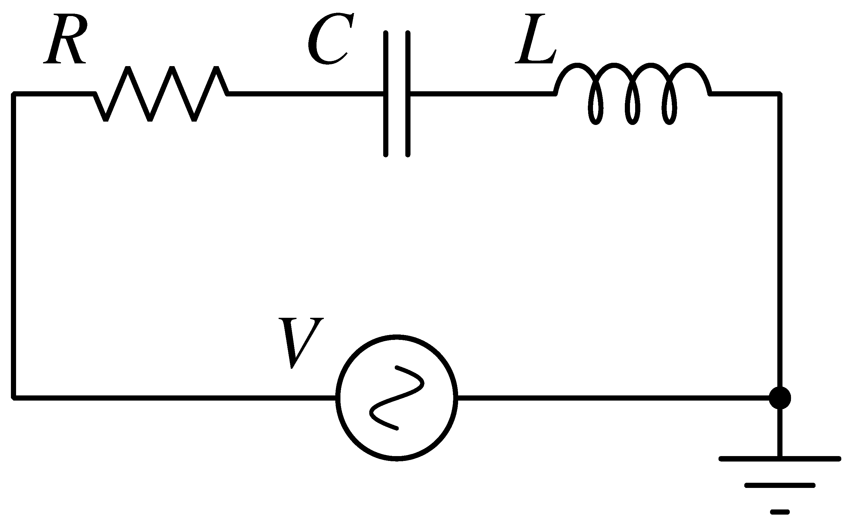
Consider the HFD equation modeled by the RLC circuit:
where
denotes the HFD,
represents the current,
is the input voltage,
is the resistance-inductance product,
is the capacitance-inductance product,
is a constant. The values of
,
,
, and
are 4, 2, 5, and 10, respectively.
where
and
are initial conditions. RLC circuits serve various purposes in signal processing and audio electronics, often employed in filter design. Configurable as low-pass, high-pass, band-pass, or band-stop filters, they play a crucial role in radio receivers for frequency tuning. Moreover, RLC circuits find application in control systems, efficiently reducing oscillations and maintaining feedback loop stability.
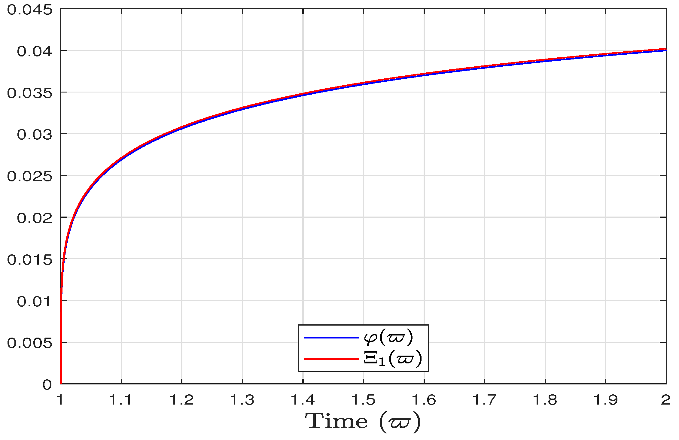
To initiate the trajectory simulation in both examples of Systems (39) and (41), we set step size
. With the choosing parameters
in Example 1 and
in Example 2, we show in Figure 2 and Figure 3 the trajectory simulation of
(blue) and
(red). Hence, we can see from Figure 2 and Figure 3 that the solution trajectory of the inequations (27) almost coincides with that of System (39). It follows that the distance between
and
is less than a constant, which shows that System (39) and (41) are UH stable according to Definition 4.

Figure 2.
Trajectory simulation of
(blue) and
(red) of System (39) on the interval [1,2] for
.
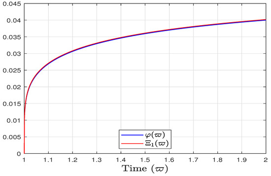
Figure 3.
Trajectory simulation of
(blue) and
(red) of System (41) on the interval [1,2] for
.
6. Conclusions
This study investigates the existence and uniqueness of solutions to the RLC circuit equation using Schaefer’s fixed point theorem and Banach’s contraction principle. It investigates Ulam-type stability results for fractional Hadamard-IDEs applied to the RLC model with nonlocal boundary conditions. By using advanced mathematical techniques, this research improves our understanding of stability and solution properties in fractional calculus and provides insights into complex dynamical systems. Through rigorous analysis, the study aims to shed light on the behavior and properties of these equations. Numerical examples validate the theoretical findings and improve practical understanding and applicability. The solutions depend on symmetric parameters that fulfill certain conditions. The RLC circuit model is analyzed using the fixed point approach, which ensures the existence and uniqueness of the solution under conditions derived from Banach contraction and Schaefer’s theorem. Future research could extend the stability analysis to multi-component and higher-order systems, and develop advanced numerical methods for solving Hadamard fractional differential equations. Applications in diverse domains such as control theory and biological systems, along with real-world implementations in engineering, could validate and expand the practical utility of this work.
Author Contributions
Conceptualization, M.M.; Methodology, S.S. and M.M.; Formal analysis, R.R. and M.R.; Investigation, S.S. and M.R.; Writing—original draft, M.M. and S.S.; Writing—review and editing, M.R. and R.R.; Supervision, S.S. and R.R. All authors have read and agreed to the published version of the manuscript.
Funding
M. Rhaima was supported by Researchers Supporting Project number (RSPD2024R683) King Saud University, Riyadh, Saudi Arabia. The second author gratefully acknowledge this work is funded by the Centre for Nonlinear Systems, Chennai Institute of Technology (CIT), India, vide funding number CIT/CNS/2024/RP-005.
Informed Consent Statement
Not applicable.
Data Availability Statement
No data were used for the research described in the article.
Conflicts of Interest
The authors declare no conflicts of interest.
References
- Sudsutad, W.; Ntouyas, S.K.; Tariboon, J. Systems of fractional Langevin equations of Riemann-Liouville and Hadamard types. Adv. Differ. Equ. 2015, 2015, 1–24. [Google Scholar] [CrossRef]
- Ntouyas, S.K.; Sitho, S.; Khoployklang, T.; Tariboon, J. Sequential Riemann–Liouville and Hadamard–Caputo fractional differential equation with iterated fractional integrals conditions. Axioms 2021, 10, 277. [Google Scholar] [CrossRef]
- Borisut, P.; Kumam, P.; Ahmed, I.; Sitthithakerngkiet, K. Nonlinear Caputo fractional derivative with nonlocal Riemann-Liouville fractional integral condition via fixed point theorems. Symmetry 2019, 11, 829. [Google Scholar] [CrossRef]
- Shah, K.; Arfan, M.; Ullah, A.; Al-Mdallal, Q.; Ansari, K.J.; Abdeljawad, T. Computational study on the dynamics of fractional order differential equations with applications. Chaos Solitons Fractals 2022, 157, 111955. [Google Scholar] [CrossRef]
- Mohamed, S.A. A fractional differential quadrature method for fractional differential equations and fractional eigenvalue problems. Math. Methods Appl. Sci. 2020. [Google Scholar] [CrossRef]
- Dzherbashian, M.; Nersesian, A. Fractional derivatives and Cauchy problem for differential equations of fractional order. Fract. Calc. Appl. Anal. 2020, 23, 1810–1836. [Google Scholar] [CrossRef]
- Sevinik Adigüzel, R.; Aksoy, Ü.; Karapinar, E.; Erhan, İ.M. On the solution of a boundary value problem associated with a fractional differential equation. Math. Methods Appl. Sci. 2020. [Google Scholar] [CrossRef]
- Jalili, B.; Jalili, P.; Shateri, A.; Ganji, D.D. Rigid plate submerged in a Newtonian fluid and fractional differential equation problems via Caputo fractional derivative. Partial Differ. Equ. Appl. Math. 2022, 6, 100452. [Google Scholar] [CrossRef]
- Ding, W.; Patnaik, S.; Sidhardh, S.; Semperlotti, F. Applications of distributed-order fractional operators: A review. Entropy 2021, 23, 110. [Google Scholar] [CrossRef]
- Tlelo-Cuautle, E.; Pano-Azucena, A.D.; Guillén-Fernández, O.; Silva-Juárez, A. Analog/Digital Implementation of Fractional Order Chaotic Circuits and Applications; Springer: Berlin/Heidelberg, Germany, 2020. [Google Scholar]
- Yang, F.; Mou, J.; Liu, J.; Ma, C.; Yan, H. Characteristic analysis of the fractional-order hyperchaotic complex system and its image encryption application. Signal Process. 2020, 169, 107373. [Google Scholar] [CrossRef]
- Wang, S.; He, S.; Yousefpour, A.; Jahanshahi, H.; Repnik, R.; Perc, M. Chaos and complexity in a fractional-order financial system with time delays. Chaos Solitons Fractals 2020, 131, 109521. [Google Scholar] [CrossRef]
- Shanmugam, S.; Narayanan, G.; Rajagopal, K.; Ali, M.S. Finite-time synchronization of complex-valued neural networks with reaction-diffusion terms: An adaptive intermittent control approach. Neural Comput. Appl. 2024, 36, 7389–7404. [Google Scholar] [CrossRef]
- Ahmad, S.; Ullah, A.; Akgül, A. Investigating the complex behaviour of multi-scroll chaotic system with Caputo fractal-fractional operator. Chaos Solitons Fractals 2021, 146, 110900. [Google Scholar] [CrossRef]
- Klimek, M. Sequential fractional differential equations with Hadamard derivative. Commun. Nonlinear Sci. Numer. Simul. 2011, 16, 4689–4697. [Google Scholar] [CrossRef]
- Gohar, M.; Li, C.; Li, Z. Finite difference methods for Caputo–Hadamard fractional differential equations. Mediterr. J. Math. 2020, 17, 194. [Google Scholar] [CrossRef]
- Benkerrouche, A.; Souid, M.S.; Karapınar, E.; Hakem, A. On the boundary value problems of Hadamard fractional differential equations of variable order. Math. Methods Appl. Sci. 2023, 46, 3187–3203. [Google Scholar] [CrossRef]
- Guo, L.; Li, C.; Zhao, J. Existence of Monotone Positive Solutions for Caputo–Hadamard Nonlinear Fractional Differential Equation with Infinite-Point Boundary Value Conditions. Symmetry 2023, 15, 970. [Google Scholar] [CrossRef]
- Subramanian, M.; Manigandan, M.; Gopal, T.N. Fractional differential equations involving Hadamard fractional derivatives with nonlocal multi-point boundary conditions. Discontinuity Nonlinearity Complex. 2020, 9, 421–431. [Google Scholar] [CrossRef]
- Manigandan, M.; Subramanian, M.; Duraisamy, P.; Gopal, T.N. On Caputo-Hadamard type fractional differential equations with nonlocal discrete boundary conditions. Discontinuity Nonlinearity Complex. 2021, 10, 185–194. [Google Scholar] [CrossRef]
- Van Mieghem, P. Origin of the fractional derivative and fractional non-Markovian continuous-time processes. Phys. Rev. Res. 2022, 4, 023242. [Google Scholar] [CrossRef]
- Li, C.; Zhu, C.; Zhang, N.; Sui, S.; Zhao, J. Free vibration of self-powered nanoribbons subjected to thermal-mechanical-electrical fields based on a nonlocal strain gradient theory. Appl. Math. Model. 2022, 110, 583–602. [Google Scholar] [CrossRef]
- Zhu, C.; Chen, Y.; Zhao, J.; Li, C.; Lei, Z. On Nonlocal Vertical and Horizontal Bending of a Micro-Beam. Math. Probl. Eng. 2022, 2022, 5121377. [Google Scholar] [CrossRef]
- Garra, R.; Orsingher, E.; Polito, F. A note on Hadamard fractional differential equations with varying coefficients and their applications in probability. Mathematics 2018, 6, 4. [Google Scholar] [CrossRef]
- Fan, E.; Li, C.; Li, Z. Numerical approaches to Caputo–Hadamard fractional derivatives with applications to long-term integration of fractional differential systems. Commun. Nonlinear Sci. Numer. Simul. 2022, 106, 106096. [Google Scholar] [CrossRef]
- Mirzaee, F.; Samadyar, N. Extension of Darbo fixed-point theorem to illustrate existence of the solutions of some nonlinear functional stochastic integral equations. Int. J. Nonlinear Anal. Appl. 2020, 11, 413–421. [Google Scholar]
- Al Elaiw, A.; Awadalla, M.; Manigandan, M.; Abuasbeh, K. A novel implementation of Mönch’s fixed point theorem to a system of nonlinear Hadamard fractional differential equations. Fractal Fract. 2022, 6, 586. [Google Scholar] [CrossRef]
- Karapınar, E.; Abdeljawad, T.; Jarad, F. Applying new fixed point theorems on fractional and ordinary differential equations. Adv. Differ. Equ. 2019, 2019, 1–25. [Google Scholar] [CrossRef]
- Shen, G.; Sakthivel, R.; Ren, Y.; Li, M. Controllability and stability of fractional stochastic functional systems driven by Rosenblatt process. Collect. Math. 2020, 71, 63–82. [Google Scholar] [CrossRef]
- Almutairi, A.; El-Metwally, H.; Sohaly, M.; Elbaz, I. Lyapunov stability analysis for nonlinear delay systems under random effects and stochastic perturbations with applications in finance and ecology. Adv. Differ. Equ. 2021, 2021, 1–32. [Google Scholar]
- Shen, G.; Xiao, R.; Yin, X. Averaging principle and stability of hybrid stochastic fractional differential equations driven by Lévy noise. Int. J. Syst. Sci. 2020, 51, 2115–2133. [Google Scholar] [CrossRef]
- Abdo, M.S.; Panchal, S.K.; Wahash, H.A. Ulam–Hyers–Mittag-Leffler stability for a ψ-Hilfer problem with fractional order and infinite delay. Results Appl. Math. 2020, 7, 100115. [Google Scholar] [CrossRef]
- Arshad, U.; Sultana, M.; Ali, A.H.; Bazighifan, O.; Al-Moneef, A.A.; Nonlaopon, K. Numerical solutions of fractional-order electrical rlc circuit equations via three numerical techniques. Mathematics 2022, 10, 3071. [Google Scholar] [CrossRef]
- Lavenda, B. Concepts of stability and symmetry in irreversible thermodynamics. I. Found. Phys. 1972, 2, 161–179. [Google Scholar] [CrossRef]
- Gallavotti, G. Breakdown and regeneration of time reversal symmetry in nonequilibrium statistical mechanics. Phys. D Nonlinear Phenom. 1998, 112, 250–257. [Google Scholar] [CrossRef]
- Russo, G.; Slotine, J.J.E. Symmetries, stability, and control in nonlinear systems and networks. Phys. Rev. E 2011, 84, 041929. [Google Scholar] [CrossRef]
- Kilbas, A.A.; Srivastava, H.M.; Trujillo, J.J. Theory and Applications of Fractional Differential Equations; Elsevier: Amsterdam, The Netherlands, 2006; Volume 204. [Google Scholar]
- Qassim, M.; Furati, K.M.; Tatar, N.E. On a differential equation involving Hilfer-Hadamard fractional derivative. In Abstract and Applied Analysis; Hindawi: London, UK, 2012; Volume 2012, p. 391062. [Google Scholar]
- Rus, I.A. Ulam Stability of Ordinary Differential Equations; Studia Universitatis Babes-Bolyai, Mathematica: Cluj-Napoca, Romania, 2009. [Google Scholar]
Disclaimer/Publisher’s Note: The statements, opinions and data contained in all publications are solely those of the individual author(s) and contributor(s) and not of MDPI and/or the editor(s). MDPI and/or the editor(s) disclaim responsibility for any injury to people or property resulting from any ideas, methods, instructions or products referred to in the content. |
© 2024 by the authors. Licensee MDPI, Basel, Switzerland. This article is an open access article distributed under the terms and conditions of the Creative Commons Attribution (CC BY) license (https://creativecommons.org/licenses/by/4.0/).